1 Introduction
Ciliated protozoa emerged as an evolutionary group more than one billion years ago (Prescott Reference Prescott1994), and the habitat of ciliates is diverse: they reside in oceans, lakes, ponds, underground water, soils (Foissner, Chao & Katz Reference Foissner, Chao and Katz2008), the gills of fish (Maeda Reference Maeda1985) and the digestive tract of mammals (Newbold et al. Reference Newbold, Fuente, Belanche, Ramos-Morales and McEwan2015). Due to the considerable influence of ciliates in nature, their behaviour has been investigated intensively. Some ciliates exhibit biological reactions when their bodies are mechanically agitated. For example, in the case of Paramecium, a mechanical stimulus applied to the anterior part of the cell body causes a transient increase in membrane permeability to calcium (Naitoh & Eckert Reference Naitoh and Eckert1969). The calcium current induces a transient depolarization of the membrane, resulting in a reversal in the direction of the ciliary beat. When a swimming Paramecium bumps into a wall or another cell at its anterior end, the cell firstly swims backward, before gyrating about its posterior end and then resuming normal forward locomotion; this is known as an avoiding reaction (Eckert Reference Eckert1972; Kung Reference Kung, Chang, Satow, van Houten and Hansma1975; Naitoh & Sugino Reference Naitoh and Sugino1984; Ishikawa & Hota Reference Ishikawa and Hota2006). A mechanical stimulus applied to the posterior part of the cell body increases permeability to potassium ions (Naitoh & Eckert Reference Naitoh and Eckert1969). The hyperpolarization results in an increase in the frequency of the ciliary beat. When a swimming Paramecium collides with a following cell at its posterior end, the cell briefly increases its forward swimming velocity, and then resumes normal forward locomotion; this is known as an escape reaction (Naitoh & Sugino Reference Naitoh and Sugino1984; Ishikawa & Hota Reference Ishikawa and Hota2006). Similar avoiding reactions have been observed in other types of ciliates, such as Tetrahymena (Onimaru et al. Reference Onimaru, Ohki, Nozawa and Naitoh1980), and even in microalgae Chlamydomonas (Fujiu et al. Reference Fujiu, Nakayama, Iida, Sokabe and Yoshimura2011). The mechanosensing mechanism has been intensively investigated from a biological standpoint (Martinac, Saimi & Kung Reference Martinac, Saimi and Kung2008; Reuter, Stuermer & Plattner Reference Reuter, Stuermer and Plattner2013; Plattner Reference Plattner2017), but it is still not well understood.
Recent studies have shown that changes in the force profile of a cell membrane can trigger a conformational change in mechanosensitive ion channels (Kung Reference Kung2005). A large-conductance mechanosensitive channel of prokaryotes responds to changes in membrane tension during severe osmotic challenges, by opening a wide water-filled pore (Sukharev et al. Reference Sukharev, Blount, Martinac and Kung1997; Perozo et al. Reference Perozo, Cortes, Sompornpisut, Kloda and Martinac2002). Pak et al. proposed a multiscale continuum model to investigate the dynamic opening/closing of a mechanosensitive channel in a vesicle membrane. Ishikawa & Kikuchi (Reference Ishikawa and Kikuchi2018) investigated the deformation of Tetrahymena, and reported considerable deformation of the cell body (approximately 10 % of the body width) when the cell showed the avoiding reaction between flat plates. However, the details of the mechanisms regulating the mechanosensitive ion channels of ciliates are still unclear. Therefore, in this study, we focus on isotropic membrane tension, which is one of the most basic force profiles in a cell membrane.
Modelling a ciliate is a massive undertaking. A cell membrane contains many transmembrane proteins, some of which are anchored to cytoskeletons. Therefore, it is not straightforward to mathematically describe the rheological properties of the membrane, so an analytical model would need to include a large number of simplifications. The ciliate model used in this paper is primitive and many non-biological assumptions are made. We use the simplest model that can swim, deform and exert membrane tension, such that hydrodynamic interactions can be analysed non-trivially.
In previous analytical studies, the deformability of swimming objects was explicitly taken into account. Ohta & Ohkuma (Reference Ohta and Ohkuma2009) developed a general mathematical model of deformable self-propelled particles, in which shape deformation was assumed to be induced by the translational motion. This model has been employed for investigating swimming motion, spinning motion, collective motions, cell crawling, swimming bacteria, and the effects of external flow and the diffusion of particles (Matsuo, Tanimoto & Sano Reference Matsuo, Tanimoto and Sano2013; Ohta Reference Ohta2017; Tarama Reference Tarama2017). Motion and deformation of active fluid droplets were investigated by Whitfield & Hawkins (Reference Whitfield and Hawkins2016). Their results showed spontaneous transitions to motility and deformation, resembling the dynamics of the cell cytoskeleton in animal cells. Gao & Li (Reference Gao and Li2017) also showed that a deformable droplet encapsulating motile active particles can be driven into motion. Löber, Ziebert & Aranson (Reference Löber, Ziebert and Aranson2015) presented a phase-field model to describe the movement of interacting crawling cells. Avron, Gat & Kenneth (Reference Avron, Gat and Kenneth2004) reported optimal deformation of a two-dimensional swimming amoeboid. Misbah and colleagues investigated three-dimensional amoeboids swimming in unbounded fluid, as well as in confined geometries (Farutin et al. Reference Farutin, Rafai, Dysthe, Duperray, Peyla and Misbah2013; Wu et al. Reference Wu, Thiébaud, Hu, Farutin, Rafaï, Lai, Peyla and Misbah2015, Reference Wu, Farutin, Hu, Thiébaud, Rafaï, Peyla, Lai and Misbah2016). Morita, Omori & Ishikawa (Reference Morita, Omori and Ishikawa2018a,Reference Morita, Omori and Ishikawab) analysed the migration of a deformable microcapsule swimmer. These studies all illustrated the important effects of particle deformability on solitary and collective motions. However, the models may not be applicable to a swimming ciliate and some of them did not consider near-field hydrodynamic interactions between swimmers.
Previously, we developed a simple mathematical model for a swimming ciliate (Ishikawa et al. Reference Ishikawa, Tanaka, Imai, Omori and Matsunaga2016). A ciliate was modelled as a capsule with a hyperelastic membrane enclosing a Newtonian fluid, and the thrust generated by cilia was modelled as torque distributed above the cell body. The effects of membrane elasticity, the aspect ratio, and the density mismatch on the solitary swimming were investigated. This study extends this investigation to consider two-body interactions. By considering interactions between two cells, we are able to examine the membrane tension between them when they are almost in contact. We believe that this is a natural next step to improve mechanical understanding of the biological reactions of ciliates, even though the ciliate model used is very simple. Moreover, the way in which the deformability of cells affects the hydrodynamic interaction between microswimmers can be addressed based on the present problem setting.
In § 2, we describe the ciliate model, presenting basic equations and our numerical methods. In § 3, we show simulation results with various interaction settings, and investigate trajectories and membrane tension. In § 4, we discuss the biological implications of our results, by comparing them to those of our former experiments using Paramecium (Ishikawa & Hota Reference Ishikawa and Hota2006). Finally, we present our conclusions in § 5.
2 Basic equations and numerical methods
The basic equations describing our ciliate model are similar to our previous study (Ishikawa et al. Reference Ishikawa, Tanaka, Imai, Omori and Matsunaga2016), so we explain them only briefly here.
2.1 Deformable torque swimmer
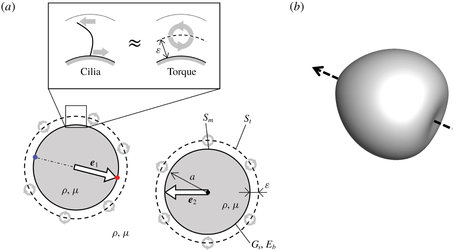
The ciliate model consists of a membrane enclosing a Newtonian fluid, and the thrust generated by cilia is modelled as torque distributed above the cell body (cf. figure 1a). The simple model includes swimming and deformation, and exerts membrane tension, so that hydrodynamic interactions can be analysed non-trivially.
A torque swimmer. (a) Schematic diagram of torque swimmers and the problem setting. The torque swimmer consists of a membrane that has a spherical reference shape with radius  $a$, a shear elastic modulus
 $G_{s}$ and a bending modulus
 $E_{b}$, enclosing a fluid with viscosity
 $\unicode[STIX]{x1D707}$ and density
 $\unicode[STIX]{x1D70C}$. A torque surface, expressed by the broken line, is placed
 $\unicode[STIX]{x1D700}$ above the membrane. For simplicity, the viscosity and density of the external and internal fluids are equal. The straight arrow
 $\boldsymbol{e}$ in the cell indicates the orientation vector, and the curved arrows on the torque surface indicate torque. (b) Three-dimensional shape of the torque swimmer with
 $Ca=0.1$. The arrow indicates the orientation vector.

The reference shape of the membrane is assumed to be a sphere with radius  $a$. We define the unit orientation vector,
 $\boldsymbol{e}$, along the line connecting two material points that exist at the posterior and anterior poles of the reference shape. The thickness of the cell membrane is small compared to the cell size and curvature radius, such that the membrane can be modelled as a two-dimensional hyperelastic surface, with surface shear elastic modulus
 $G_{s}$, area dilation modulus
 $K_{s}$ and bending modulus
 $E_{b}$. For simplicity, internal and external fluids of the membrane are assumed to have the same viscosity,
 $\unicode[STIX]{x1D707}$, and density,
 $\unicode[STIX]{x1D70C}$.
Since the traction force acting on the surrounding fluid and the reaction force transmitted to the cell membrane act in opposite directions with the same magnitude (cf. figure 1a), the effective and recovery strokes of the ciliary beat are modelled by torques distributed above the cell body. We assume that the torques are exerted at a distance  $\unicode[STIX]{x1D700}$ above the membrane, regardless of the membrane deformation; this is referred to as the torque surface. The length scale of
 $\unicode[STIX]{x1D700}$ is approximately half the length of the cilia. The strength of torque per unit reference area is assumed to be homogeneous and time invariant. The unsteadiness of the ciliary beat and the inhomogeneity in cilia distribution are ignored. The beat direction is assumed to be in the meridian direction in the reference shape, from the anterior end to the posterior end; thus, the torque vectors are oriented in the latitude direction.
When the membrane is deformed, the strengths and the directions of torques are changed as follows. Let  $\boldsymbol{x}$ be a material point at the membrane with the outward normal unit vector
 $\boldsymbol{n}(\boldsymbol{x})$. The corresponding point at the torque surface
 $\boldsymbol{x}^{\prime }$ is given by
 $\boldsymbol{x}^{\prime }=\boldsymbol{x}+\unicode[STIX]{x1D700}\boldsymbol{n}(\boldsymbol{x})$. The torque strength per unit area at
 $\boldsymbol{x}^{\prime }$ is determined by
 $L(\boldsymbol{x}^{\prime })=L_{0}(\boldsymbol{x}^{\prime })(\unicode[STIX]{x0394}A_{t,0})/(\unicode[STIX]{x0394}A_{t})|_{x^{\prime }}$, where
 $L_{0}$ is the torque strength per unit area of the reference shape, and the last fraction indicates areal ratio of the reference to the deformed torque surface at
 $\boldsymbol{x}^{\prime }$. This assumption means that the local torque strength decreases/increases when the membrane is stretched/compressed. In other words, the number density of cilia is homogeneous at the reference shape, but decreases/increases when the membrane is stretched/compressed. The total amount of torque, given by
 $\int |\boldsymbol{L}|\,\text{d}S_{t}$, is kept constant regardless of the deformation, where
 $S_{t}$ denotes the torque surface. Because the number of cilia does not change with the deformation. The direction of torque at the reference shape is in the latitude direction. We assume that the torque direction in the local coordinate system along the material points is invariant, regardless of the deformation. This assumption means that the beat direction of a cilium relative to the base membrane does not change with the deformation.
2.2 Fluid mechanics
Since ciliates are small in size, we neglect the inertial effect on the internal and external flow fields, as well as the membrane deformation. The flow field is thus governed by the Stokes equation. The velocity  $\boldsymbol{v}$ at position
 $\boldsymbol{x}$ is given by the integral over the membrane surface
 $S_{m}$ and the torque surface
 $S_{t}$ of two swimmers,
 $i=1$ and 2, as (Pozrikidis Reference Pozrikidis1992)
 $$\begin{eqnarray}\boldsymbol{v}(\boldsymbol{x})=-\frac{1}{8\unicode[STIX]{x03C0}\unicode[STIX]{x1D707}}\mathop{\sum }_{i=1}^{2}\left[\int _{S_{m}}\boldsymbol{J}(\boldsymbol{x},\boldsymbol{y})\boldsymbol{\cdot }\boldsymbol{q}(\boldsymbol{y})\,\text{d}S_{m,i}(\boldsymbol{y})+\int _{S_{t}}\boldsymbol{R}(\boldsymbol{x},\boldsymbol{y})\boldsymbol{\cdot }\boldsymbol{L}(\boldsymbol{y})\,\text{d}S_{t,i}(\boldsymbol{y})\right],\end{eqnarray}$$
where  $\boldsymbol{q}$ is the load and
 $\boldsymbol{L}$ is the torque.
 $\boldsymbol{J}$ and
 $\boldsymbol{R}$ are Green’s functions, defined as
 $$\begin{eqnarray}J_{ij}=\frac{\unicode[STIX]{x1D6FF}_{ij}}{r}+\frac{r_{i}r_{j}}{r^{3}},\quad R_{ij}=\unicode[STIX]{x1D716}_{ijk}\frac{r_{k}}{r^{3}},\end{eqnarray}$$
where  $\unicode[STIX]{x1D750}$ is the unit alternating isotropic tensor,
 $\boldsymbol{r}=\boldsymbol{x}-\boldsymbol{y}$ and
 $r=|\boldsymbol{r}|$. The dynamic condition requires that the load,
 $\boldsymbol{q}$, be equal to the viscous traction jump across the membrane
 $$\begin{eqnarray}\boldsymbol{q}(\boldsymbol{y})=[\unicode[STIX]{x1D748}_{out}(\boldsymbol{y})-\unicode[STIX]{x1D748}_{in}(\boldsymbol{y})]\boldsymbol{\cdot }\boldsymbol{n}(\boldsymbol{y}),\end{eqnarray}$$
where  $\boldsymbol{n}$ is the outward normal vector, and
 $\unicode[STIX]{x1D748}_{in}$ and
 $\unicode[STIX]{x1D748}_{out}$ are the stress tensors of the internal and external fluids, respectively.
2.3 Membrane mechanics
Let  $\boldsymbol{X}$ and
 $\boldsymbol{x}(\boldsymbol{X},t)$ be a material point on the membrane in the reference and deformed states, respectively. The surface deformation gradient tensor
 $\unicode[STIX]{x1D641}_{s}$ is given by (Pozrikidis Reference Pozrikidis2010)
 $$\begin{eqnarray}\text{d}\boldsymbol{x}=\unicode[STIX]{x1D641}_{s}\boldsymbol{\cdot }\text{d}\boldsymbol{X}.\end{eqnarray}$$
Local deformation of the membrane can be expressed by the Green–Lagrange strain tensor:
 $$\begin{eqnarray}\unicode[STIX]{x1D640}={\textstyle \frac{1}{2}}(\unicode[STIX]{x1D641}_{s}^{\text{T}}\boldsymbol{\cdot }\unicode[STIX]{x1D641}_{s}-\boldsymbol{I}_{s}),\end{eqnarray}$$
where  $\boldsymbol{I}_{s}$ is the tangential projection operator. Two invariants of the in-plane strain tensor
 $\unicode[STIX]{x1D640}$ are given by
 $$\begin{eqnarray}\displaystyle I_{1}=\unicode[STIX]{x1D706}_{1}^{2}+\unicode[STIX]{x1D706}_{2}^{2}-2,\quad I_{2}=\unicode[STIX]{x1D706}_{1}^{2}\unicode[STIX]{x1D706}_{2}^{2}-1=J_{s}^{2}-1, & & \displaystyle\end{eqnarray}$$
where  $\unicode[STIX]{x1D706}_{1}$ and
 $\unicode[STIX]{x1D706}_{2}$ are the principal stretch ratios. The Jacobian
 $J_{s}=\unicode[STIX]{x1D706}_{1}\unicode[STIX]{x1D706}_{2}$, expresses the ratio of the deformed to the reference surface area.
The membrane is modelled as an isotropic and hyperelastic material. The surface load  $\boldsymbol{q}$ in (2.1) consists of two components, i.e.
 $\boldsymbol{q}=\boldsymbol{q}_{s}+\boldsymbol{q}_{b}$, where
 $\boldsymbol{q}_{s}$ is the load due to the membrane in-plane stretch and
 $\boldsymbol{q}_{b}$ is the bending resistance. Load due to the in-plane stretch
 $\boldsymbol{q}_{s}$ is obtained from a local equilibrium equation for the Cauchy tension
 $\unicode[STIX]{x1D749}$ as
 $$\begin{eqnarray}\boldsymbol{q}_{s}=\unicode[STIX]{x1D735}_{s}\boldsymbol{\cdot }\unicode[STIX]{x1D749},\end{eqnarray}$$
where  $\unicode[STIX]{x1D735}_{s}$ is the surface gradient operator. The Cauchy tension is related to the elastic strain energy per unit area
 $W_{s}(I_{1},I_{2})$ as
 $$\begin{eqnarray}\unicode[STIX]{x1D749}=\frac{1}{J_{s}}\unicode[STIX]{x1D641}_{s}\boldsymbol{\cdot }\frac{\unicode[STIX]{x2202}W_{s}(I_{1},I_{2})}{\unicode[STIX]{x2202}\unicode[STIX]{x1D640}}\boldsymbol{\cdot }\unicode[STIX]{x1D641}_{s}^{\text{T}}.\end{eqnarray}$$
We assumed that a ciliate membrane showed strain-hardening properties with a high resistance to areal change. To express these mechanical properties, we used the two-dimensional constitutive law of Skalak et al. (Reference Skalak, TozereN, Zarda and Chien1973) given by
 $$\begin{eqnarray}W_{s}=\frac{G_{s}}{4}(I_{1}^{2}+2I_{1}-2I_{2}+CI_{2}^{2}).\end{eqnarray}$$
The area dilation modulus  $K_{s}$ can be described as
 $K_{s}=G_{s}(1+2C)$. The value of
 $C$ determines the strength of the areal incompressibility. We used
 $C=10$ throughout this study (cf. Walter, Salsac & Barthes-Biesel Reference Walter, Salsac and Barthes-Biesel2011); thus, the area dilation ratio was less than approximately 18 % for our parameter range.
Bending stiffness is based upon a model proposed by Helfrich (Reference Helfrich1973), and the bending energy  $W_{b}$ is expressed as
 $$\begin{eqnarray}W_{b}=\frac{E_{b}}{2}\int (2H-c_{0})\,\text{d}S,\end{eqnarray}$$
where  $H$ is the mean curvature of the surface and
 $c_{0}$ is the spontaneous curvature. We assume that the two layers of the lipid membrane are symmetric, i.e.
 $c_{0}=0$; thus, the energy can be converted to a force density
 $\boldsymbol{q}_{b}$ (Ou-Yang & Helfrich Reference Ou-Yang and Helfrich1989), as
 $$\begin{eqnarray}\boldsymbol{q}_{b}=-2E_{b}[\unicode[STIX]{x1D6E5}_{S}H+2H(H^{2}-K)]\boldsymbol{n},\end{eqnarray}$$
where  $\unicode[STIX]{x1D6E5}_{S}$ is the Laplace–Beltrami operator on the surface, and
 $K$ is the Gaussian curvature.
2.4 Numerical method
We used essentially the same numerical method as Walter et al. (Reference Walter, Salsac, Barthes-Biesel and Tallec2010) and Ishikawa et al. (Reference Ishikawa, Tanaka, Imai, Omori and Matsunaga2016), where the Stokes flows of the internal and external fluid are solved using a boundary element method. A computational mesh was generated on the membrane and the torque surface, and the Lagrangian positions of the membrane material points  $\boldsymbol{x}(\boldsymbol{X},t)$ were tracked over time.
Based on the virtual work principle, equation (2.7) can be rewritten in the weak form as
 $$\begin{eqnarray}\int _{S_{m}}\hat{\boldsymbol{u}}\boldsymbol{\cdot }\boldsymbol{q}_{s}\,\text{d}S_{m}=\int _{S_{m}}\hat{\unicode[STIX]{x1D73A}}\boldsymbol{ : }\unicode[STIX]{x1D749}\,\text{d}S_{m},\end{eqnarray}$$
where  $\hat{\boldsymbol{u}}$ and
 $\hat{\unicode[STIX]{x1D73A}}=\frac{1}{2}(\unicode[STIX]{x1D735}_{\boldsymbol{s}}\hat{\boldsymbol{u}}+\unicode[STIX]{x1D735}_{\boldsymbol{s}}\hat{\boldsymbol{u}}^{\text{T}})$ are the virtual displacement and strain, respectively. A finite element method was used to solve equations (2.11) and (2.12), and the viscous load
 $\boldsymbol{q}$ for a given membrane deformation was derived. Substituting
 $\boldsymbol{q}$ into (2.1) resulted in a new velocity field
 $\boldsymbol{v}$, which was calculated by a boundary element method. Once the velocity field
 $\boldsymbol{v}$ had been computed, the membrane material point
 $\boldsymbol{x}$ was updated using the kinematic condition,
 $\unicode[STIX]{x2202}\boldsymbol{x}/\unicode[STIX]{x2202}t=\boldsymbol{v}(\boldsymbol{x},t)$, via a second-order Runge–Kutta method.
The membrane was discretized by 20 480 triangular elements with 10 242 nodes. The effect of the mesh resolution was explicitly discussed in Ishikawa et al. (Reference Ishikawa, Tanaka, Imai, Omori and Matsunaga2016). A computational mesh was then generated for the torque surface based upon the membrane mesh using the equation  $\boldsymbol{x}^{\prime }=\boldsymbol{x}+\unicode[STIX]{x1D700}\boldsymbol{n}(\boldsymbol{x})$, where
 $\unicode[STIX]{x1D700}=0.05a$. Although equation (2.1) rigorously satisfies the divergence-free conditions of the flow field, numerical errors accumulated over an extended time period may cause slight changes in the volume of the internal fluid. To overcome this, we followed the method of Freund (Reference Freund2007), keeping a constant internal volume by iteratively modifying the node positions. The volume change of a capsule remained smaller than 0.01% throughout the study. To avoid overlapping of the swimmers, we did not implement any artificial interparticle force in the simulation. When the torque surface
 $S_{t}$ of one cell overlapped with the membrane surface
 $S_{m}$ of another cell, we simply stopped the computation.
The capillary number  $(Ca)$ represents the ratio of viscous to elastic force, implying that the deformation of a swimmer increases as
 $Ca$ is increased. Note that
 $Ca$ is dimensionless and defined by
 $Ca=(\unicode[STIX]{x1D707}U_{0})/G_{s}$, where
 $U_{0}$ is the velocity of a torque swimmer with
 $Ca=0.001$, showing little deformation. Torque strength per unit reference area,
 $L$, was fixed regardless of
 $Ca$. All equations were non-dimensionalized using the characteristic velocity
 $U_{0}$, radius
 $a$, viscosity
 $\unicode[STIX]{x1D707}$, shear elastic modulus
 $G_{s}$ and bending modulus
 $E_{b}$. Here,
 $Be$ (also dimensionless) represents the ratio of bending to elastic force, defined by
 $Be=(\unicode[STIX]{x1D707}E_{b})/(a^{2}G_{s})$. We set
 $Be=0.01$, to focus on in-plane elastic tension.
The capillary number of an actual ciliate is difficult to estimate, because the cell structure is not as simple as a capsule. Here, we attempt to roughly estimate it by using the available data in the literature. The shear elastic modulus  $G_{s}$ can be correlated to Young’s modulus
 $E$ as
 $G_{s}=Eh$, where
 $h$ is the membrane thickness. Besides, in a micropipette aspiration experiment, the suction pressure
 $\unicode[STIX]{x0394}P$ can be expressed as
 $\unicode[STIX]{x0394}P=2\unicode[STIX]{x03C0}E\ell \unicode[STIX]{x1D719}/(3a_{p})$ (cf. Hochmuth Reference Hochmuth2000), where
 $\ell$ is the aspiration length,
 $a_{p}$ is the pipette radius and
 $\unicode[STIX]{x1D719}$ is a coefficient related to the pipette shape. Campillo et al. (Reference Campillo, Fisch, Jerber, Desforges, Dupuis-Williams, Nassoy and Sykes2012) performed the micropipette aspiration experiments using a Paramecium. When they applied the suction pressure of 1 kPa, the aspiration length of the cell cortex was approximately
 $10~\unicode[STIX]{x03BC}\text{m}$. By inserting these values with
 $a_{p}=3.5~\unicode[STIX]{x03BC}\text{m}$ and
 $\unicode[STIX]{x1D719}=2.1$, we obtain the Young’s modulus of approximately
 $E=80~\text{Pa}$. By assuming the effective thickness of the cell cortex to be in the range
 $0.1{-}10~\unicode[STIX]{x03BC}\text{m}$,
 $Ca$ of Paramecium, swimming with the velocity of
 $2~\text{mm}~\text{s}^{-1}$ in fluid with viscosity
 $10^{-3}~\text{Pa}~\text{s}$, may be estimated in the rage 0.25–0.0025.
3 Results
In this section, we investigate four kinds of configurations in the two-body interactions: (a) face-to-face interaction, (b) side-by-side interaction, (c) crossing interaction, and (d) chasing interaction.
3.1 Face-to-face interaction
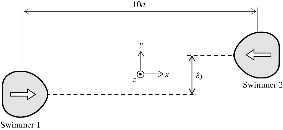
Figure 2 shows the initial configuration of face-to-face interactions. Swimmers are initially  $10a$ apart in the
 $x$-direction with an offset of
 $\unicode[STIX]{x1D6FF}y$ in the
 $y$-direction. The orientation vector of swimmer 1 is in the positive
 $x$-direction, whereas that of swimmer 2 is in the negative
 $x$-direction. The centre positions and orientation vectors of the two swimmers exist in the same
 $x$–
 $y$ plane, and tend to remain in the same
 $x$–
 $y$ plane during the interaction due to symmetry.
Initial configuration of the face-to-face interaction. Swimmers are  $10a$ apart in the
 $x$-direction with an offset of
 $\unicode[STIX]{x1D6FF}y$ in the
 $y$-direction.

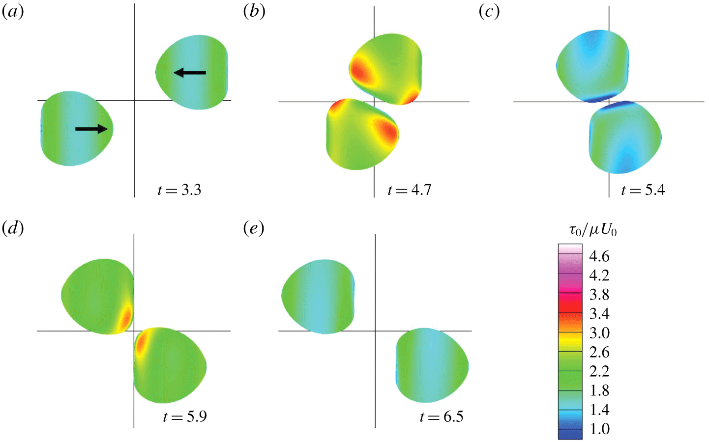
Before getting close during the face-to-face interaction, the swimmer with  $Ca=0.1$ deforms to a heart shape (figure 3a). Similar heart-shaped deformation was also reported for a solitary swimmer (Ishikawa et al. Reference Ishikawa, Tanaka, Imai, Omori and Matsunaga2016). During the interaction, swimmers deform in particular in the near-contact region. The colour in figure 3 indicates the in-plane isotropic tension
 $\unicode[STIX]{x1D70F}_{0}$, defined by
 $\unicode[STIX]{x1D70F}_{0}=(\unicode[STIX]{x1D70F}_{1}+\unicode[STIX]{x1D70F}_{2})/2$, where
 $\unicode[STIX]{x1D70F}_{1}$ and
 $\unicode[STIX]{x1D70F}_{2}$ are the principal tensions. Here,
 $\unicode[STIX]{x1D70F}_{0}$ is isotropic in direction, so it can be regarded as two-dimensional pressure. We see that
 $\unicode[STIX]{x1D70F}_{0}$ becomes large in the anterior side when the two swimmers are in close proximity (figure 3b), because high pressure is generated between the two near-contact surfaces. We observe the isotropic tension decrease once (figure 3c), because the high pressure disappears, before increasing again (figure 3d) because the membrane is stretched by the low pressure between the two near-contact surfaces.
Sequences showing the interaction between two facing swimmers with $\unicode[STIX]{x1D6FF}y=1.5a$ (with
 $Ca=0.1$). Colour contours show the in-plane isotropic tension
 $\unicode[STIX]{x1D70F}_{0}$.

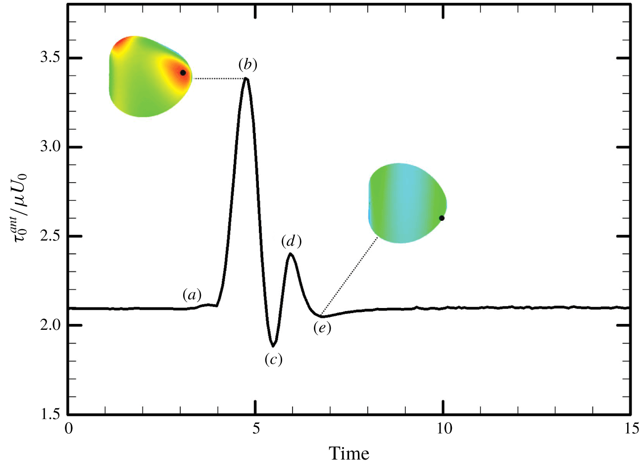
In Ishikawa & Hota (Reference Ishikawa and Hota2006), Paramecium in a face-to-face configuration occasionally showed an avoiding reaction. Therefore, we calculate the maximum isotropic tension in the anterior  $1/3$ region of the body,
 $\unicode[STIX]{x1D70F}_{0}^{ant}$, and plot it as a function of time in figure 4. Large tension is generated when the two cells come into close proximity, indicated by point (b). The position of maximum
 $\unicode[STIX]{x1D70F}_{0}^{ant}$ is not exactly at the anterior tip, instead being slightly offset, as indicated by the black dot.
The time change of the maximum value of in-plane isotropic tension in the anterior region,  $\unicode[STIX]{x1D70F}_{0}^{ant}$ (with
 $\unicode[STIX]{x1D6FF}y=1.5a$ and
 $Ca=0.1$). Panels (a–e) correspond to the instances in figure 3, and the black dots indicate the position of maximum
 $\unicode[STIX]{x1D70F}_{0}^{ant}$ on the membrane.

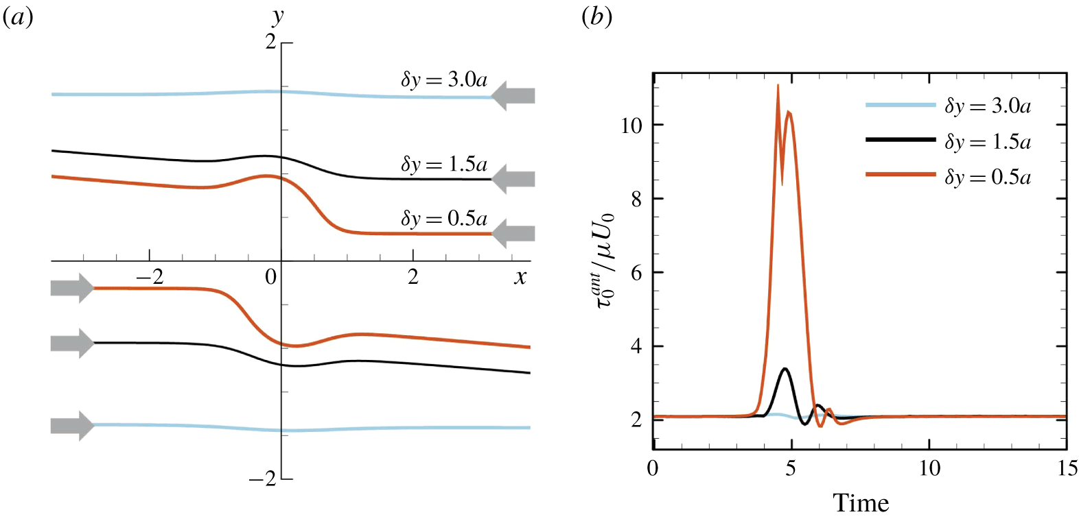
Figure 5(a) shows the effect of initial offset  $\unicode[STIX]{x1D6FF}y$ on the trajectory of a swimmer’s volumetric centre
 $(Ca=0.1)$. A small
 $\unicode[STIX]{x1D6FF}y$ has a considerable influence on the trajectory. The face-to-face interaction induces not only drift in the centre positions, but also a change in the cell’s orientation. We note that similar drift of centre positions was reported for interactions between two inert capsules in background shear flow (Lac, Morel & Barthes-Biesel Reference Lac, Morel and Barthes-Biesel2007). The inert capsules tended to drift away from each other, similar to the torque swimmers; however, no orientation vector was defined for the inert capsules. The maximum value of in-plane isotropic tension in the anterior region
 $\unicode[STIX]{x1D70F}_{0}^{ant}$ is strongly influenced by
 $\unicode[STIX]{x1D6FF}y$ (figure 5b). When
 $\unicode[STIX]{x1D6FF}y=0.5a$,
 $\unicode[STIX]{x1D70F}_{0}^{ant}$ becomes more than five times larger than the steady value during solitary swimming.
The effect of initial offset  $\unicode[STIX]{x1D6FF}y$ in the face-to-face interaction (with
 $Ca=0.1$). (a) Trajectories of the volumetric centre of a swimmer, and (b) the maximum value of in-plane isotropic tension in the anterior region,
 $\unicode[STIX]{x1D70F}_{0}^{ant}$.

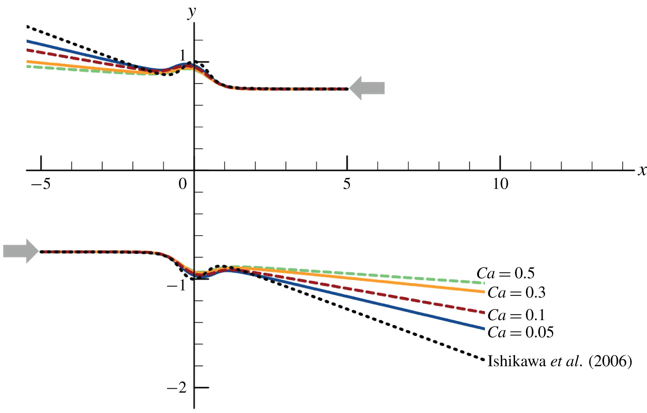
Figure 6 shows the effect of deformability,  $Ca$, on the trajectories of the volumetric centres of swimmers (
 $\unicode[STIX]{x1D6FF}y=1.5a$). To compare our results with those of the velocity squirmer model (see appendix A; Lighthill (Reference Lighthill1952), Blake (Reference Blake1971)), we also plotted the trajectories of the spherical velocity squirmers obtained in Ishikawa, Simmonds & Pedley (Reference Ishikawa, Simmonds and Pedley2006), indicated as dashed curves in the figure. The change in orientation of swimmers is reduced as
 $Ca$ increases. Since the scattering angle of cells after the interaction affects the diffusion of a cell suspension, the deformability also plays a role in the macroscopic self-diffusivity.
The effect of  $Ca$ on the trajectories of the volumetric centre of a swimmer (with
 $\unicode[STIX]{x1D6FF}y=1.5a$). The dashed curve is the trajectory of spherical velocity squirmers (Ishikawa et al. Reference Ishikawa, Simmonds and Pedley2006) with second-mode squirming
 $\unicode[STIX]{x1D6FD}=0$.

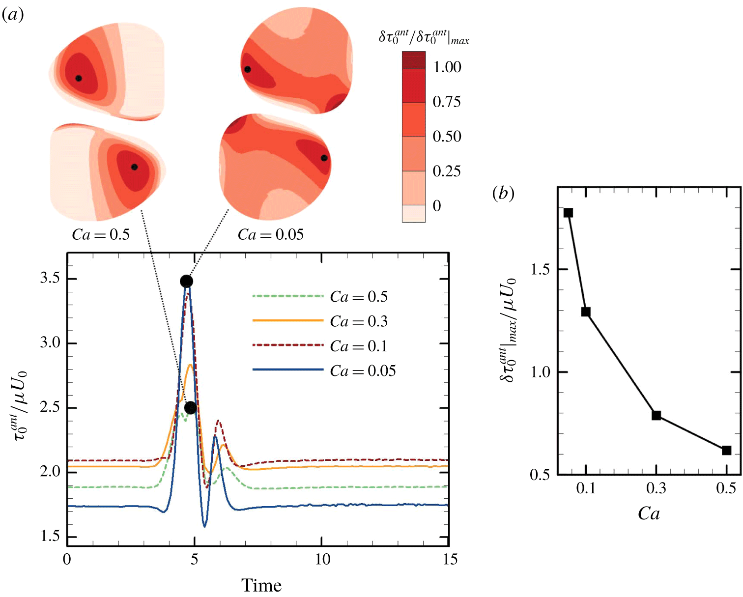
The effect of deformability,  $Ca$, on the maximum value of in-plane isotropic tension in the anterior region,
 $\unicode[STIX]{x1D70F}_{0}^{ant}$, is shown in figure 7 (
 $\unicode[STIX]{x1D6FF}y=1.5a$). By changing
 $Ca$, the steady value of
 $\unicode[STIX]{x1D70F}_{0}^{ant}$ during solitary swimming, i.e. the baseline, is also changed. As
 $Ca$ is decreased,
 $\unicode[STIX]{x1D70F}_{0}^{ant}$ increases from the baseline. These results indicate that stiffer cells experience larger isotropic tension during the interactions. When
 $Ca=0.5$, the position of maximum
 $\unicode[STIX]{x1D70F}_{0}^{ant}$ has a large offset from the
 $x$–
 $y$ plane of symmetry. This result illustrates that the position of maximum
 $\unicode[STIX]{x1D70F}_{0}^{ant}$ does not correspond to the near-contact position, and thus mechanical stimulation can be sensed by a cell at a different location than the near-contact region.
The effect of  $Ca$ on the maximum value of in-plane isotropic tension in the anterior region
 $\unicode[STIX]{x1D70F}_{0}^{ant}$ (with
 $\unicode[STIX]{x1D6FF}y=1.5a$). (a) Time change of
 $\unicode[STIX]{x1D70F}_{0}^{ant}$. Insets show the swimmers when
 $\unicode[STIX]{x1D70F}_{0}^{ant}$ is at the maximum during the interaction with
 $Ca=0.5$ and 0.05, where the black dots indicate the position of maximum
 $\unicode[STIX]{x1D70F}_{0}^{ant}$ on the membrane. (b) The effect of
 $Ca$ on the increase of the maximum value of
 $\unicode[STIX]{x1D70F}_{0}^{ant}$ from the baseline.

3.2 Side-by-side interaction
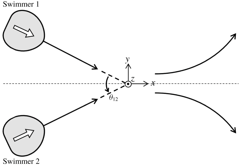
Figure 8 shows the initial configuration of side-by-side interactions, in which swimmer 2 is the mirror image of swimmer 1 with respect to the  $y=0$ plane. The centre positions and orientation vectors of two swimmers exist in the same
 $x$–
 $y$ plane, and tend to remain in the same
 $x$–
 $y$ plane during the interaction due to symmetry. Here,
 $\unicode[STIX]{x1D703}_{12}$ is the angle between the two swimmers’ orientation vectors.
Initial configuration of side-by-side interactions. Here,  $\unicode[STIX]{x1D703}_{12}$ is defined as the angle between the orientation vectors of two swimmers.

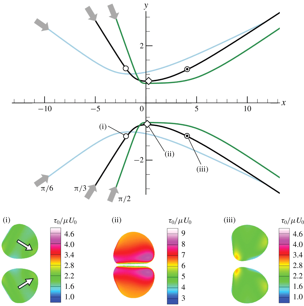
The trajectories of the swimmers with the initial angle of  $\unicode[STIX]{x1D703}_{12}^{ini}=\unicode[STIX]{x03C0}/6,\unicode[STIX]{x03C0}/3$ and
 $\unicode[STIX]{x03C0}/2$ are shown in figure 9
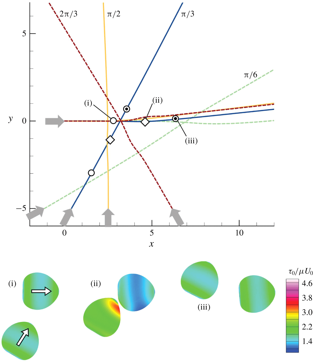
 $(Ca=0.1)$. The cells firstly come into close proximity with each other, then swim side-by-side for a while without collision, and finally swim away from each other, in all cases. We note that a similar side-by-side interaction was also observed in an experiment using Paramecium (cf. Ishikawa & Hota Reference Ishikawa and Hota2006). The insets of figure 9 show the distribution of isotropic tension
 $\unicode[STIX]{x1D70F}_{0}$ at three different positions in the case of
 $\unicode[STIX]{x1D703}_{12}^{ini}=\unicode[STIX]{x03C0}/3$. Large
 $\unicode[STIX]{x1D70F}_{0}$ is generated on the whole body when cells are side-by-side at (ii) because of high pressure between the two near-contact surfaces. The high pressure induces membrane deformation to prevent direct collision of cells.
The effect of initial angle  $\unicode[STIX]{x1D703}_{12}^{ini}$ on the trajectories of the volumetric centre of a swimmer (with
 $Ca=0.1$). The insets show the distribution of
 $\unicode[STIX]{x1D70F}_{0}$ at three positions, (i), (ii) and (iii), with
 $\unicode[STIX]{x1D703}_{12}^{ini}=\unicode[STIX]{x03C0}/3$.

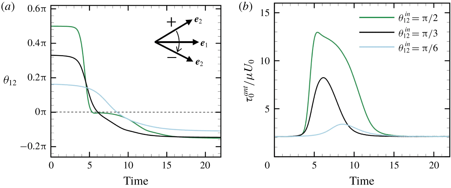
The time change in the relative orientation of cells is shown in figure 10(a). Initially,  $\unicode[STIX]{x1D703}_{12}^{ini}$ has positive values of
 $\unicode[STIX]{x03C0}/6,\unicode[STIX]{x03C0}/3$ or
 $\unicode[STIX]{x03C0}/2$. After the interaction, the sign of
 $\unicode[STIX]{x1D703}_{12}$ becomes negative, indicating that the cells are directed away from each other. The final value of
 $\unicode[STIX]{x1D703}_{12}$ is similar regardless of
 $\unicode[STIX]{x1D703}_{12}^{ini}$. However, the isotropic tension in the anterior region,
 $\unicode[STIX]{x1D70F}_{0}^{ant}$, takes different values depending on
 $\unicode[STIX]{x1D703}_{12}^{ini}$. This is because larger
 $\unicode[STIX]{x1D703}_{12}^{ini}$ generates higher pressure between the two near-contact surfaces, which results in large membrane tension, even though the trajectories were not strongly affected by the pressure.
The effect of initial angle  $\unicode[STIX]{x1D703}_{12}^{ini}$ on the interaction of swimmers (with
 $Ca=0.1$). (a) Time change of
 $\unicode[STIX]{x1D703}_{12}$, and (b) time change of
 $\unicode[STIX]{x1D70F}_{0}^{ant}$.

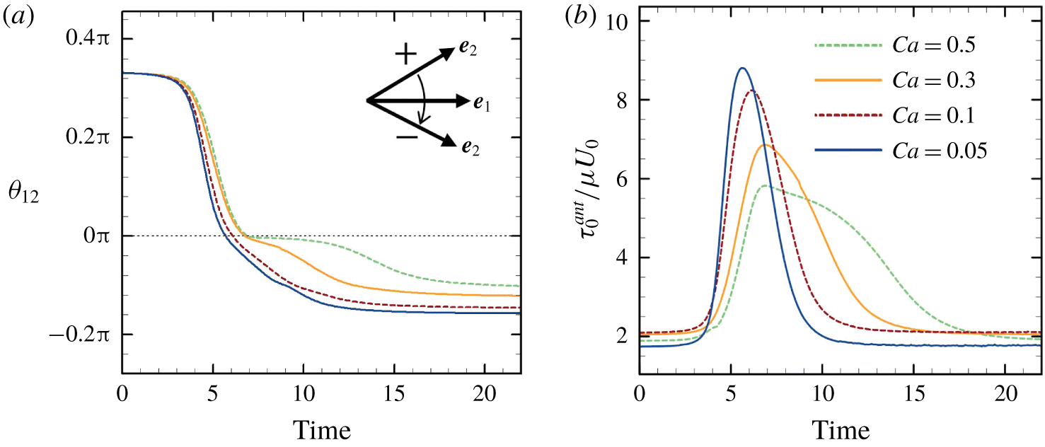
Figure 11(a) shows the effect of deformability,  $Ca$, on the relative orientation of cells (
 $\unicode[STIX]{x1D703}_{12}^{ini}=\unicode[STIX]{x03C0}/3$). The final angle slightly decreases as
 $Ca$ is increased. The decrease in scattering angle may cause a decrease in the self-diffusivity of cells in the suspension. Isotropic tension in the anterior region,
 $\unicode[STIX]{x1D70F}_{0}^{ant}$, is also influenced by
 $Ca$. Note that
 $\unicode[STIX]{x1D70F}_{0}^{ant}$ decreases as
 $Ca$ is increased (figure 11b).
The effect of  $Ca$ on the interaction of swimmers (with
 $\unicode[STIX]{x1D703}_{12}^{ini}=\unicode[STIX]{x03C0}/3$). (a) Time change of
 $\unicode[STIX]{x1D703}_{12}$, and (b) time change of
 $\unicode[STIX]{x1D70F}_{0}^{ant}$.

3.3 Crossing interaction
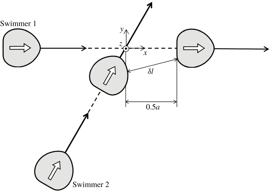
Figure 12 shows the initial configuration of crossing interactions. Swimmer 1 is initially oriented in the  $x$-direction, whereas swimmer 2 has a relative orientation angle of
 $\unicode[STIX]{x1D703}_{12}^{ini}$. To ensure their paths cross, we use an offset of
 $0.5a$ compared to the side-by-side interaction. In this case, the posterior region of swimmer 1 and the anterior region of swimmer 2 come into close contact.
Initial configuration of crossing interactions, during which there is an offset of  $0.5a$ compared to the side-by-side interaction. Here,
 $\unicode[STIX]{x1D6FF}l$ is the minimum separation distance between the membranes of two swimmers.

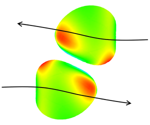
The trajectories of a swimmer’s volumetric centres with  $\unicode[STIX]{x1D703}_{12}^{ini}=\unicode[STIX]{x03C0}/6,\unicode[STIX]{x03C0}/3,\unicode[STIX]{x03C0}/2$ and
 $2\unicode[STIX]{x03C0}/3$ are shown in figure 13
 $(Ca=0.1)$. None of the trajectories are strongly affected by the interactions because of the offset of
 $0.5a$. The insets in the figure show the distribution of
 $\unicode[STIX]{x1D70F}_{0}$ at three positions, (i), (ii) and (iii), with
 $\unicode[STIX]{x1D703}_{12}^{ini}=\unicode[STIX]{x03C0}/3$. Although
 $\unicode[STIX]{x1D70F}_{0}$ has changed considerably at position (ii), the trajectory has not, because the strong interaction only occurs over a short time period.
The effect of initial angle  $\unicode[STIX]{x1D703}_{12}^{ini}$ on the trajectories of the volumetric centre of a swimmer (with
 $Ca=0.1$). The insets show the distribution of
 $\unicode[STIX]{x1D70F}_{0}$ at three positions, (i), (ii) and (iii), with
 $\unicode[STIX]{x1D703}_{12}^{ini}=\unicode[STIX]{x03C0}/3$.

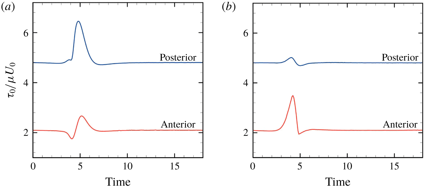
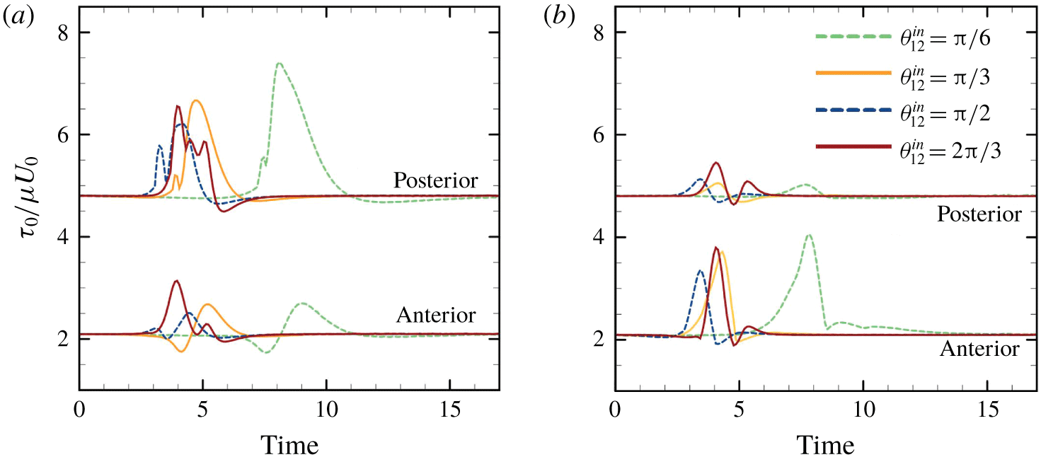
Figure 14 shows the time change of the maximum value of isotropic tension in the anterior and posterior regions ( $\unicode[STIX]{x1D703}_{12}^{ini}=\unicode[STIX]{x03C0}/3$ and
 $Ca=0.1$). Here
 $\unicode[STIX]{x1D70F}_{0}^{pos}$ is defined as the maximum
 $\unicode[STIX]{x1D70F}_{0}$ in the posterior
 $1/3$ region of the body. There is a large increase of posterior tension
 $\unicode[STIX]{x1D70F}_{0}^{pos}$ of swimmer 1 (ahead), and a large increase of anterior tension
 $\unicode[STIX]{x1D70F}_{0}^{ant}$ of swimmer 2 (behind). In Ishikawa & Hota (Reference Ishikawa and Hota2006), the Paramecium in front during the crossing interaction occasionally showed an escape reaction, while the Paramecium behind occasionally showed an avoiding reaction. The biological implications of these results are discussed in § 4.
Time change of the maximum value of isotropic tension in the anterior region  $\unicode[STIX]{x1D70F}_{0}^{ant}$ and in the posterior region
 $\unicode[STIX]{x1D70F}_{0}^{pos}$ (with
 $\unicode[STIX]{x1D703}_{12}^{ini}=\unicode[STIX]{x03C0}/3$ and
 $Ca=0.1$). (a) Swimmer 1, ahead, and (b) swimmer 2, behind.

3.4 Chasing interaction
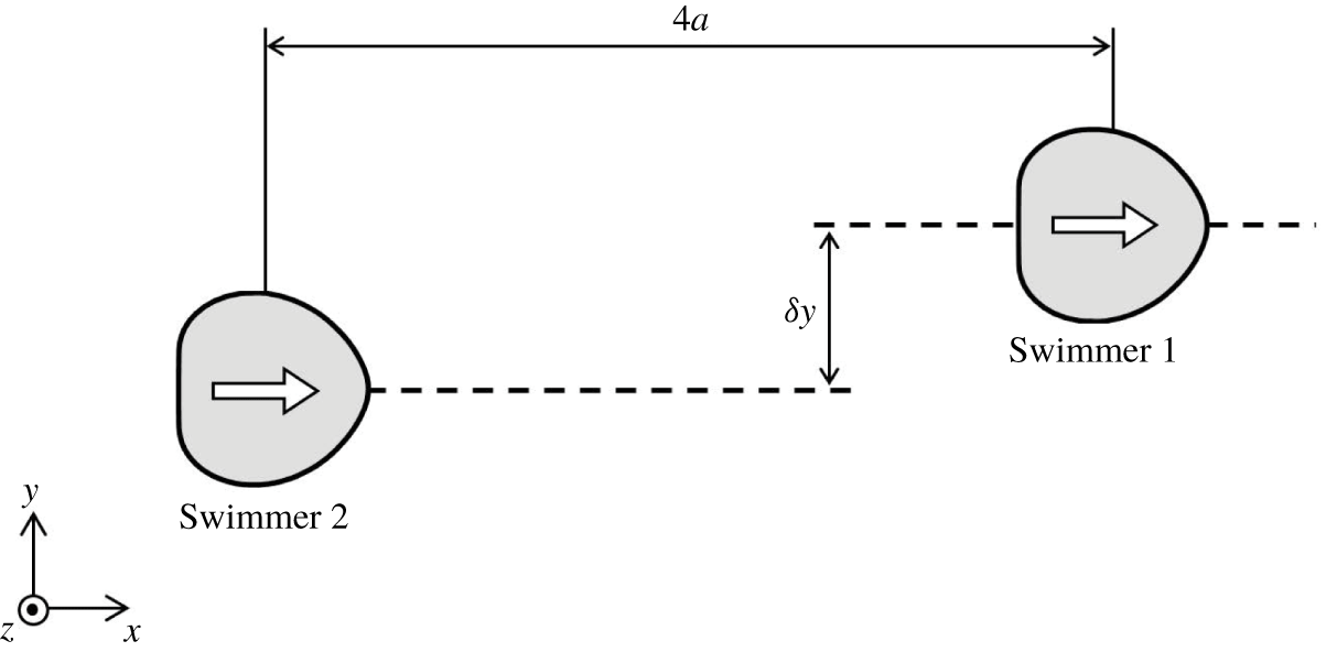
Finally, we investigate chasing interactions, in which the initial configuration is set as shown in figure 15. In former studies using the velocity squirmer model (cf. appendix A), it was found that chasing interactions are strongly affected by swimmer type (Ishikawa et al. Reference Ishikawa, Simmonds and Pedley2006). A puller has a thrust-generating apparatus in front of the body, whereas that of a pusher is behind the body. Considering the swimmer is force-free and torque-free, the leading-order singularity is the force dipole, which governs the far-field flow (Ishikawa Reference Ishikawa2009). The force dipole is positive for a puller, whereas negative for a pusher. When squirmers are pullers, i.e. the second-mode squirming  $\unicode[STIX]{x1D6FD}$ is positive, attracting velocities are generated between the fore and aft squirmers. Firstly, they tend to come into close proximity with each other, then change their orientation considerably, and eventually swim away from each other. In contrast, when the squirmers are pushers, i.e.
 $\unicode[STIX]{x1D6FD}<0$, repelling velocities are generated between the fore and aft squirmers, and the cells do not interact in the near-field, in a chasing configuration. When the squirmer is neutral, i.e.
 $\unicode[STIX]{x1D6FD}=0$, the exerted velocities are cancelled out, and there is no change in the relative position of the squirmers.
Initial configuration of chasing interactions. Swimmers are  $4a$ apart in the
 $x$-direction with an offset of
 $\unicode[STIX]{x1D6FF}y$ in the
 $y$-direction.

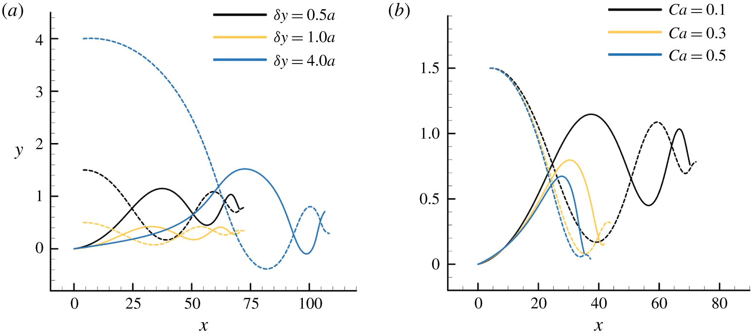
However, for deformable torque swimmers, we observed qualitatively different interactions from the velocity squirmers. The trajectories of the volumetric centre of a swimmer with various offsets  $\unicode[STIX]{x1D6FF}y\;(Ca=0.1)$ and
 $Ca\;(\unicode[STIX]{x1D6FF}y=1.5a)$ are shown in figure 16. In all the cases, the two swimmers, which are initially apart, are gradually attracted to each other via wavy trajectories. They are eventually aligned fore-and-aft, and attached to each other. At this point, we stopped the simulation to avoid the overlapping of cells. It takes longer for the cells to attach when increasing the initial offset
 $\unicode[STIX]{x1D6FF}y$, and attraction is faster when increasing the deformability
 $Ca$.
The effect of parameters on the trajectories of the volumetric centre of a swimmer. Dashed curves indicate the trajectories of swimmer 1, ahead of swimmer 2, whereas solid curves indicate trajectories of swimmer 2, behind swimmer 1. (a) The effect of  $\unicode[STIX]{x1D6FF}y$ (with
 $Ca=0.1$), and (b) the effect of
 $Ca$ (with
 $\unicode[STIX]{x1D6FF}y=1.5a$).

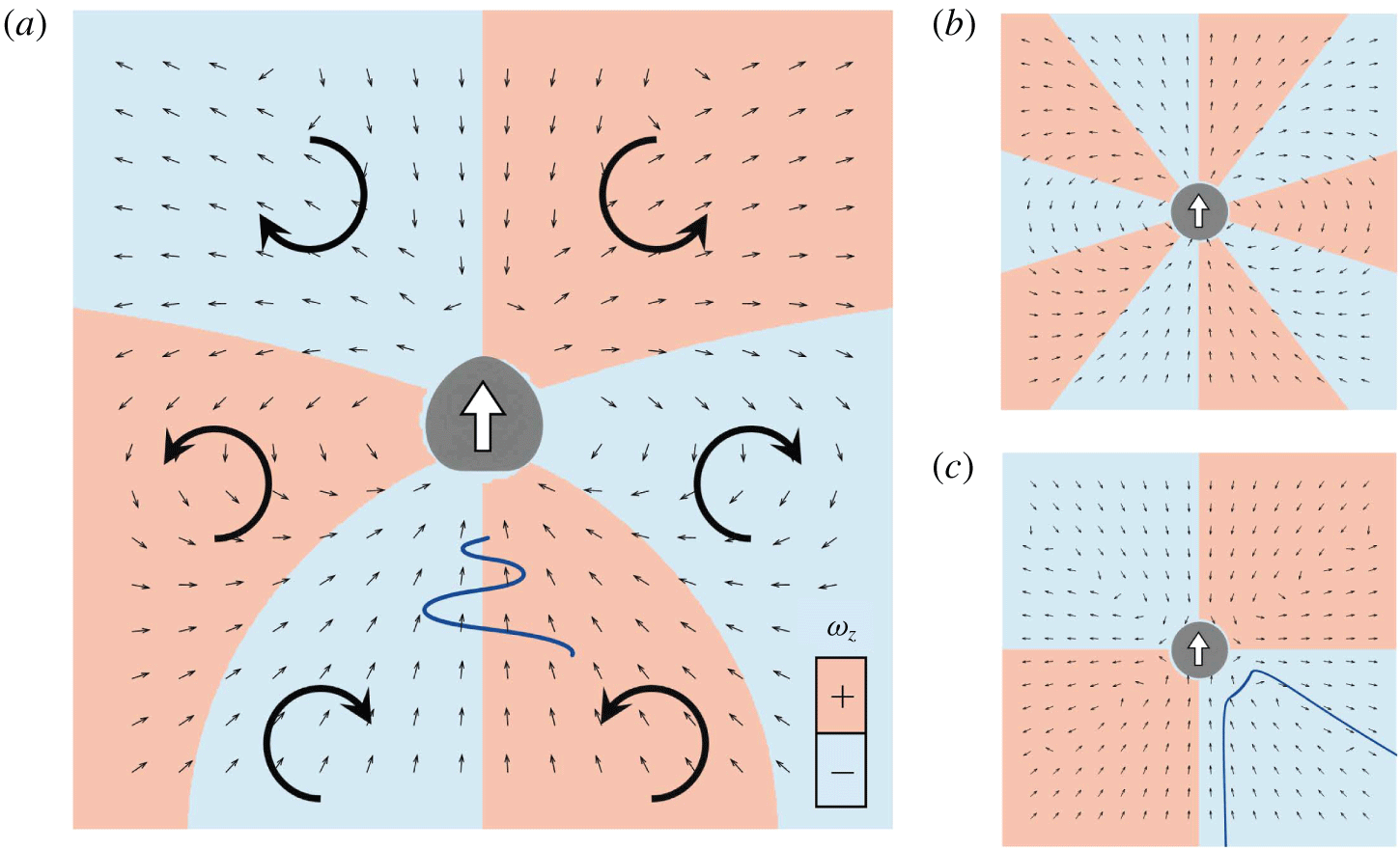
To understand the mechanism of attraction, we calculated the velocity field generated around a solitary torque swimmer with  $Ca=0.1$. Small black arrows in figure 17(a) indicate the direction of the velocity vectors in the lab frame. The attractive velocities are generated in both anterior and posterior regions of the swimmer, indicating that cells in the fore-and-aft configuration are attracted by the velocities. Red and blue colours in figure 17(a) indicate the sign of vorticity
 $\unicode[STIX]{x1D714}_{z}$. Due to the vorticity, a cell that is behind on the right-hand side is directed to the left, whereas a cell behind on the left-hand side is directed to the right. Similarly, a cell ahead on the right-hand side is directed to the left, and vice versa. In figure 17(a), the relative trajectory of swimmer 2 with
 $\unicode[STIX]{x1D6FF}y=1.5a$ is also plotted (wavy blue line), and this is consistent with the above-mentioned mechanism.
The velocity field generated around a solitary swimmer. Small black arrows indicate the direction of velocity vectors in the lab frame. Red and blue colours indicate the sign of vorticity  $\unicode[STIX]{x1D714}_{z}$. (a) Velocity field around a deformable torque swimmer with
 $Ca=0.1$. Large arrows indicate the direction of vorticity
 $\unicode[STIX]{x1D714}_{z}$. The wavy blue line indicates the relative trajectory of swimmer 2 (behind) with
 $\unicode[STIX]{x1D6FF}y=1.5a$. (b) Velocity field around a spherical velocity squirmer with a second-mode squirming of
 $\unicode[STIX]{x1D6FD}=0$. (c) Velocity field around a spherical velocity squirmer with a second-mode squirming of
 $\unicode[STIX]{x1D6FD}=5$. The blue curve indicates the relative trajectory of squirmer 2 (behind) with
 $\unicode[STIX]{x1D6FF}y=a$ (Ishikawa et al. Reference Ishikawa, Simmonds and Pedley2006).

For the conventional velocity squirmer model, the velocity field around a solitary squirmer is generated as shown in figure 17(b,c). When the squirmers are neutral (figure 17b), the disturbed velocity fields cancel out each other, and there is no change in the relative position or orientation of squirmers. When the squirmers are pullers (figure 17c) a squirmer that is behind is attracted by the squirmer ahead, but the interaction is unstable in terms of the orientation. The relative trajectories of squirmers with  $\unicode[STIX]{x1D6FD}=5$ draws them away from each other, as shown by the blue curve (cf. Ishikawa et al. Reference Ishikawa, Simmonds and Pedley2006). The deformability of swimmers stabilizes the chasing interaction and enables them to swim as a fore–aft dumbbell pair.
4 Discussions
In this section, we discuss the biological implications of our results, comparing them to our former experiments using Paramecium (Ishikawa & Hota Reference Ishikawa and Hota2006). Firstly, we describe the advantages and disadvantages of the current cell model. The main advantage is its simplicity, which allows us to analyse the interaction and deformation of cells rigorously by using fluid and solid mechanics. This simplicity also allows us to apply the present model as a general model of deformable microswimmers, so that the knowledge obtained in this study may be useful in understanding the interactions of active droplets and vesicles. The simplicity of the model, however, presents some drawbacks when discussing actual biological phenomena, such as mechanosensing mechanisms. In reality, the surface of a ciliate is covered by hundreds of motile cilia, and the cell membrane also covers the ciliary axoneme structures. Such detailed biological structure is omitted in this study, making it difficult to quantitatively compare our results with other experiments. Moreover, the mechanosensing mechanism of Paramecium has not yet been fully clarified, so some uncertainties remain in biological responses with regard to the in-plane isotropic tension,  $\unicode[STIX]{x1D70F}_{0}$. Considering these drawbacks, our discussion becomes qualitative due to the simplicity of the modelling.
The side-by-side swimming of two Paramecium was observed by Ishikawa & Hota (Reference Ishikawa and Hota2006), in which the two cells tended to swim side-by-side at first, and then moved away from each other at an acute angle. The final angle of approximately 0.4 rad was independent of the initial angle. Our results showed similar side-by-side interactions (cf. figure 9). The final angles shown in figures 10 and 11 were within the range  $0.3-0.5$ rad, consistent with the experimental results.
The rate at which an escape reaction happened during crossing interactions was investigated in Ishikawa & Hota (Reference Ishikawa and Hota2006). It was found that approximately 20 % of Paramecium that were ahead showed an escape reaction regardless of the initial angle  $\unicode[STIX]{x1D703}_{12}^{ini}$, and the maximum rate of escape reaction occurred when
 $\unicode[STIX]{x1D703}_{12}^{ini}=\unicode[STIX]{x03C0}/2$. To reproduce the experimental settings, we performed a simulation of crossing interactions with varying
 $\unicode[STIX]{x1D703}_{12}^{ini}$. To focus on the effect of initial angle
 $\unicode[STIX]{x1D703}_{12}^{ini}$, we adjusted the offset of swimmer 2 (figure 12) to achieve a minimum separation distance between the two membranes of the two swimmers during the interaction in the range
 $\unicode[STIX]{x1D6FF}l=0.069a\sim 0.07a$, regardless of
 $\unicode[STIX]{x1D703}_{12}^{ini}$. The results of isotropic tension,
 $\unicode[STIX]{x1D70F}_{0}$, of swimmer 1 are shown in figure 18(a). The tension in the posterior region
 $\unicode[STIX]{x1D70F}_{0}^{pos}$ of the swimmer that is ahead is considerably increased regardless of
 $\unicode[STIX]{x1D703}_{12}^{ini}$. This result is consistent with the experimental observations, in which approximately 20 % of Paramecium that were ahead had an escape reaction regardless of the initial angle
 $\unicode[STIX]{x1D703}_{12}^{ini}$. The maximum
 $\unicode[STIX]{x1D70F}_{0}^{pos}$ appeared when
 $\unicode[STIX]{x1D703}_{12}^{ini}=\unicode[STIX]{x03C0}/2$ in the simulation, which is again consistent with the experimental results.
The effect of the initial angle  $\unicode[STIX]{x1D703}_{12}^{ini}$ on the maximum value of isotropic tension in the anterior region
 $\unicode[STIX]{x1D70F}_{0}^{ant}$ and the posterior region
 $\unicode[STIX]{x1D70F}_{0}^{pos}$, in which the minimum separation distance
 $\unicode[STIX]{x1D6FF}l$ during the interaction is set in the range
 $\unicode[STIX]{x1D6FF}l=0.069a\sim 0.07a$ (with
 $Ca=0.1$). (a) Swimmer 1 (ahead), and (b) swimmer 2 (behind).

The rate at which an avoiding reaction occurred in crossing interactions was also investigated in Ishikawa & Hota (Reference Ishikawa and Hota2006). It was found that most of the Paramecium that were behind did not show the avoiding reaction. Figure 18(b) shows the simulation results of isotropic tension  $\unicode[STIX]{x1D70F}_{0}$ of swimmer 2, which was behind. The increase of
 $\unicode[STIX]{x1D70F}_{0}^{ant}$ of the swimmer behind, and that of
 $\unicode[STIX]{x1D70F}_{0}^{pos}$ of the swimmer ahead are of similar magnitude. In the experiment, however, the rate of escape reaction was approximately 20 %, whereas that having an avoiding reaction was less than 3 %. These results indicate that Paramecium are more sensitive to mechanical stimulation in the posterior versus anterior region. We speculate that the sensitivity plays a role in predator–prey interactions, because predators may approach the prey from behind.
5 Conclusions
In this study, we investigated hydrodynamic interactions between two deformable microswimmers and quantified the membrane tension during the interaction. We examined four kinds of configurations: (a) face-to-face interaction, (b) side-by-side interaction, (c) crossing interaction, and (d) chasing interaction. By increasing the deformability  $Ca$, membrane tension during the interaction was decreased, and cells tended to have smaller scattering angles after the interaction. These results are in line with that of rigid velocity squirmer models, indicating that the velocity squirmer model could be regarded as the small
 $Ca$ limit of the model in this study. For the case of chasing interactions, swimmers attracted each other due to membrane deformability. It was found that the deformability of the swimmers makes two-body interactions qualitatively different in this case. Finally, we discussed the biological implications of our results, comparing them to our former experiments using Paramecium (Ishikawa & Hota Reference Ishikawa and Hota2006). The rate of escape and avoiding reactions during crossing interactions was found to be qualitatively consistent with the experiments. The knowledge obtained in this study is useful for understanding the effects of swimmer deformability in hydrodynamic interactions, and provides a theoretical basis for investigating a mechanical picture of the biological reactions of ciliates.
Acknowledgements
This research was supported by the Japan Society for the Promotion of Science Grant-in-Aid for Scientific Research (JSPS KAKENHI grant no. 17H00853).
Declaration of interests
The authors report no conflict of interest.
Appendix A. Velocity squirmer model
In this appendix, we present a description of the velocity squirmer model, which was first proposed by Lighthill (Reference Lighthill1952) and has been extended by Blake (Reference Blake1971). Squirming velocity on the surface of a sphere is expressed as
 $$\begin{eqnarray}u_{r}|_{r=a}=\mathop{\sum }_{n}A_{n}(t)P_{n}(\cos \unicode[STIX]{x1D703}),\quad u_{\unicode[STIX]{x1D703}}|_{r=a}=\mathop{\sum }_{n}B_{n}(t)V_{n}(\cos \unicode[STIX]{x1D703}),\end{eqnarray}$$
where  $a$ is the radius,
 $A_{n}(t)$ and
 $B_{n}(t)$ are coefficients of
 $n^{th}$ mode,
 $P_{n}$ is the
 $n^{th}$ Legendre polynomial and
 $V_{n}$ is defined as
 $$\begin{eqnarray}V_{n}(\cos \unicode[STIX]{x1D703})=\frac{2}{n(n+1)}\sin \unicode[STIX]{x1D703}P_{n}^{\prime }(\cos \unicode[STIX]{x1D703}).\end{eqnarray}$$
Here,  $u_{r}$ and
 $u_{\unicode[STIX]{x1D703}}$ are the velocities in the
 $r$ and
 $\unicode[STIX]{x1D703}$ directions in spherical polar coordinates. The spherical coordinates are defined such that
 $\unicode[STIX]{x1D703}=0$ and
 $\unicode[STIX]{x1D703}=\unicode[STIX]{x03C0}$ denote the axis of symmetry and thus the swimming direction.
In Ishikawa et al. (Reference Ishikawa, Simmonds and Pedley2006), we assumed that the squirmer has a rigid spherical body with a purely tangential surface velocity, i.e.  $A_{n}=0$. We also omitted squirming modes higher than the second mode, i.e.
 $B_{n}=0$ when
 $n\geqslant 3$. The ratio of second- to first-mode squirming was defined as
 $\unicode[STIX]{x1D6FD}$, i.e.
 $\unicode[STIX]{x1D6FD}=B_{2}/B_{1}$. A squirmer with positive
 $\unicode[STIX]{x1D6FD}$ is a puller for which the thrust-generating apparatus is in front of the body, whereas a squirmer with negative
 $\unicode[STIX]{x1D6FD}$ is a pusher for which the thrust-generating apparatus is behind the body. When
 $\unicode[STIX]{x1D6FD}=0$, no dipole is generated by the squirmer, and it is called a neutral squirmer.