





1. Introduction
In flows dominated by inertia, inertial turbulence (IT) is known to be highly intermittent (Pomeau & Manneville Reference Pomeau and Manneville1980; Staicu & van de Water Reference Staicu and van de Water2003; Avila & Hof Reference Avila and Hof2013). The addition of polymers is known to modify the flow structures near the wall and promote intermittency in both negligible (Burghelea et al. Reference Burghelea, Segre and Steinberg2007; Jun & Steinberg Reference Jun and Steinberg2017; Singh et al. Reference Singh, Perlekar, Mitra and Rosti2024) and high (Xi & Graham Reference Xi and Graham2012a
; Rosti et al. Reference Rosti, Perlekar and Mitra2023) inertia regimes. Viscoelastic turbulent flow states arising in these two limits can be broadly classified according to the Reynolds number at which they occur,
 $\textit {Re}=t_v/t_{adv}=\rho UL/\eta$
, where
 $t_v=\rho L^2/\eta$
and
 $t_{adv}=L/U$
are the viscous and advection time scales,
 $\rho$
and
 $\eta$
are the fluid density and dynamic viscosity, respectively,
 $U$
the reference fluid velocity and
 $L$
the characteristic length scale of the flow. For
 $\textit {Re}\lt 1$
, viscoelastic turbulence is driven purely by elastic effects and is referred to as elastic turbulence (ET). In contrast, for
 $\textit {Re}\geqslant 1$
, elasto-inertial turbulence (EIT) emerges due to the combination of inertial and elastic effects (Steinberg Reference Steinberg2021; Datta et al. Reference Datta2022; Dubief et al. Reference Dubief, Terrapon and Hof2023). In both cases, sufficient fluid elasticity is necessary to trigger elastic instabilities, expressed either through the Weissenberg number,
 $\textit{Wi}=t_e U/L=t_e\dot {\gamma }$
or the elasticity number,
 $\textit{El}=\textit{Wi}/\textit {Re}=t_e/t_v$
, where
 $t_e$
is the polymer relaxation and
 $\dot {\gamma }$
is the shear rate.
In ET and low-
 $\textit {Re}$
EIT, mainly driven by purely elastic instabilities, the promotion of intermittency is attributed to the accumulation of elastic stresses close to the wall boundary, sporadically injected into the flow (Burghelea et al. Reference Burghelea, Segre and Steinberg2007; Jun & Steinberg Reference Jun and Steinberg2017). This results in large skewness in the distributions of various flow parameters, such as torque, pressure, dissipation rates and velocity fluctuations or velocity differences (Burghelea et al. Reference Burghelea, Segre and Steinberg2007; Jun & Steinberg Reference Jun and Steinberg2017; Qin & Arratia Reference Qin and Arratia2017; Singh et al. Reference Singh, Perlekar, Mitra and Rosti2024). Interestingly, Qin & Arratia (Reference Qin and Arratia2017) reported that in perturbed channel flows, intermittency was only observed near the perturbation source and not further downstream, suggesting that potentially different mechanisms are at play between parallel and curvilinear shear flows.
In high-
 $\textit {Re}$
EIT, intermittency is considered part of the turbulent drag reduction (TDR) mechanism (Min et al. Reference Min, Yul Yoo, Choi and Jodeph2003; Kim et al. Reference Kim, Li, Sureshkumar, Balachandar and Adrian2007; Samanta et al. Reference Samanta, Housiadas, Handler and Beris2009). However, the interplay between elasticity and inertia in this case introduces remarkable complexity, altering both the onset mechanisms and the underlying structures compared with IT and ET (Song et al. Reference Song, Zhu, Lin, Liu and Khomami2023b
; Zhang et al. Reference Zhang, Fan, Su, Xi and Sun2025a
). Unlike IT, EIT is associated with spanwise coherent structures (such as solitary pairs, arrowheads or narwhals) (Groisman & Steinberg Reference Groisman and Steinberg1997; Dubief et al. Reference Dubief, Page, Kerswell, Terrapon and Steinberg2022; Lellep et al. Reference Lellep, Linkmann and Morozov2023), which persist over a wide range of elasticities and Reynolds numbers (Choueiri et al. Reference Choueiri, Lopez, Varshney, Sankar and Hof2021). These properties may also differ greatly between various geometries, especially when considering curvilinear and parallel shear flows. Early studies of the latter have linked the intermittent phenomena to hibernating and active turbulent events in which turbulence is either suppressed (hibernating) or promoted (active) for a short time period (Xi & Graham Reference Xi and Graham2010a
; Graham Reference Graham2014). Hibernation, in particular, is also observed in IT (Agrawal et al. Reference Agrawal, Ng, Davis, Park, Graham, Dennis and Poole2020) and is thus described as a Newtonian edge state (Graham Reference Graham2014), which becomes progressively more dominant with increasing
 $\textit{Wi}$
, while active turbulence is suppressed (Xi & Graham Reference Xi and Graham2012a
). During the hibernation events, the flow exhibits similar characteristics (low Reynolds stresses, weak vortices) to those in maximum drag reduction (MDR) (Xi & Graham Reference Xi and Graham2012a
; Lopez Reference Lopez2022), namely the maximum degree of TDR possible to achieve. The MDR has been suggested to be a flow state in which active turbulence is fully suppressed and hibernating events dominate the flow dynamics in minimal channel flows (Graham Reference Graham2014). However, this flow state was not achieved numerically by Graham (Reference Graham2014); instead, the flow relaminarised after a critical
 $\textit{El}$
, which was attributed initially to the small domain studied therein. A later study (Lopez Reference Lopez2022) argued that hibernation becomes spatio-temporal intermittency in large domains and is a signature of relaminarisation in channel flows. In this context, hibernation is considered part of a reverse transition from Newtonian turbulence to laminar flow. Despite differences in the mechanisms, there is a strong similarity between the intermittent behaviour of low- and high-
 $\textit {Re}$
turbulence in viscoelastic flows, pointing towards the universality of this phenomenon (Jun & Steinberg Reference Jun and Steinberg2017; Steinberg Reference Steinberg2021).
Intermittency has received relatively little attention in Taylor–Couette (TC) flows, where it is most often linked to the merging and splitting transition (MST)/vortex merging and splitting (VMS) route to EIT (Lopez Reference Lopez2022; Lacassagne et al. Reference Lacassagne, Cagney, Gillissen and Balabani2020; Song et al. Reference Song, Wan, Liu, Lu and Khomami2021). This is surprising, given that several transitional flow states, such as the flame pattern (FP), rotating–standing waves and disordered oscillations, are inherently chaotic and could display an intermittent dynamics (Boulafentis et al. Reference Boulafentis, Lacassagne, Cagney and Balabani2023; Latrache et al. Reference Latrache, Kelai, Bai, Crumeyrolle and Mutabazi2025). One possible reason is that most viscoelastic instabilities in TC flows arise at intermediate Reynolds numbers: lower than those associated with EIT in channel flows, yet higher than those for purely ET. This intermediate regime complicates direct comparisons with other flow geometries and may have obscured the role of intermittency.
This work presents the first investigation into the role of intermittency in viscoelastic flows at an intermediate
 $\textit {Re} = 120$
(below the onset of IT, corresponding to laminar Taylor vortex flow (TVF) in the Newtonian case) and high
 $\textit{Wi}$
. The results highlight the dual influence of viscoelasticity in curvilinear flows, even at moderate inertia: while it destabilises the base flow and promotes a transition to chaos at intermediate elasticities, it also suppresses the previously created turbulence at higher
 $\textit{Wi}$
(or
 $\textit{El}$
). Spatio-temporal intermittency is promoted by viscoelasticity and follows similar trends to flow hibernation, typically observed in much higher
 $\textit {Re}$
. Since the flow is initiated from a laminar state, the findings suggest that hibernation does not have solely Newtonian origins; instead, it is a property of turbulent flows promoted by viscoelasticity, even at intermediate
 $\textit {Re}$
. The following sections describe the materials and methods used in the experiments, outline the spatio-temporal characteristics of the flow states, quantify key flow statistics and analyse the relationship between intermittency and hibernation.
2. Materials and methods
The TC set-up shown in figure 1 has the same geometrical features as the ones used in our previous works (Cagney et al. Reference Cagney, Lacassagne and Balabani2020; Lacassagne et al. Reference Lacassagne, Cagney, Gillissen and Balabani2020, Reference Lacassagne, Boulafentis, Cagney and Balabani2021a
,
Reference Lacassagne, Cagney and Balabanib
; Boulafentis et al. Reference Boulafentis, Lacassagne, Cagney and Balabani2024a
). The inner cylinder has a radius of
 $r_i=21.66$
mm, and the outer one
 $r_o=27.92$
mm, resulting in a gap between the two cylinders of
 $d=6.26$
mm, a radius ratio of
 $\eta _{cell}=r_i/r_o =0.77$
and a curvature of
 $\epsilon =d/r_i=0.29$
. The axial length of the flow cell is
 $H=135$
mm, resulting in an aspect ratio of
 $\varGamma =H/d =21.56$
. The rotational speed of the inner cylinder (
 $\Omega_i$
) was controlled accurately using a stepper motor (SmartDrive Ltd., Cambridge, UK), with a high resolution of 52 000 microsteps/revolution. The TC cell was enclosed in a rectangular container filled with circulating water for temperature control and visualisation purposes. The temperature of the working fluids was thus maintained constant at 20
 $^{\circ}C$
.
A summary of the rheological properties of the fluids.

Table 1. Long description
Ten columns: Concentration(ppm), Entanglement State, eta0(Pa.s), eta_inf(Pa.s), n_c, t_c(ms), n_e-bar, t_e(ms), beta, El. Rows (conc, state, eta0, eta_inf, n_c, t_c, n_e-bar, t_e, beta, El): 0,none,0.078,-,-,-,1,-,1,0. 5,dilute,0.081,-,-,-,1,11.42,0.96,0.02. 10,dilute,0.084,0.837,0.076,3.2,0.998,39.3,0.93,0.07. 50,dilute,0.0849,0.0768,0.923,18,0.994,70.1,0.92,0.12. 200,dilute,0.0982,0.0908,0.4249,116.8,0.982,173.81,0.79,0.33. 300,dilute,0.1214,0.1057,0.6309,229.8,0.981,232.21,0.64,0.53. 500,dilute,0.1277,0.1069,0.4982,188.8,0.973,257.12,0.61,0.59. 700,semi-dilute,0.1394,0.0964,0.7445,283.1,0.958,275,0.56,0.64. Relaxation time and El rise, beta falls with concentration; shear-thinning stays negligible (n_e-bar>0.95).
Schematic representation of the TC cell and the particle image velocimetry (PIV) set-up.

Figure 1. Long description
A cylindrical Taylor-Couette cell in 3-D perspective: a grey rotating inner cylinder (radius r_i, angular speed Omega, curved arrow at top) sits inside a larger stationary outer cylinder (radius r_o), separated by annular gap d = r_o-r_i; cylinder height is H. A cylindrical coordinate system (r, theta, z) is shown at the base. On the left, a box labelled ‘PIV Laser’ emits a thin light sheet (highlighted green, with circular tracer-particle markers) illuminating a vertical strip of the annular gap, marking the plane where particle image velocimetry measurements are taken.
Boger fluids comprising mixtures of high molecular weight polyacrylamide (PAAM) polymers (Sigma-Aldrich, weight-average molecular weight
 $M_w=5.5\times 10^6\ \mathrm{g \boldsymbol{\,}mol^{-1}}$
) dissolved in 80 % glycerol, 20 % distilled water were employed. Different polymer concentrations (5–700 ppm) were used and the mixtures were prepared following the protocol described in Boulafentis et al. (Reference Boulafentis, Lacassagne, Cagney and Balabani2024a
). The high volume fraction of glycerol allowed us to extend the range of fluid elasticities studied (
 $\textit{El}$
= 0–0.64,
 $\textit{Wi}$
= 0–76.4) without increasing the shear-thinning nature of the fluids. The solutions were systematically characterised using steady-shear rheology in a rotational rheometer (ARES rheometer, TA instruments) equipped with a Couette geometry. The viscosity curves,
 $\eta -\dot {\gamma }$
, are shown in figure 2(a), along with the Carreau model fitting. The values obtained from the fitting are summarised in table 1 for all fluids. The density of the solutions remained constant for all fluids and equal to that of the solvent,
 $\rho$
= 1217.3
 $\mathrm{kg\,m^{-3}}$
. The average gradient of the viscosity curve,
 $\bar {n}_e$
, was calculated for all cases (table 1) and the solutions were found to illustrate negligible shear thinning (
 $\bar {n}_e\gt 0.95$
) (Cagney et al. Reference Cagney, Lacassagne and Balabani2020; Lacassagne et al. Reference Lacassagne, Cagney, Gillissen and Balabani2020).
(a) Steady-shear rheological properties of the PAAM solutions used in this work for different concentrations, (b) filament diameter evolution for different PAAM concentrations. The solvent (WGL-80) is the same for all cases, 80 % glycerol and 20 % water.

Figure 2. Long description
(a) Log-log plot of viscosity (0.05-0.3 Pa.s) vs shear rate (1-10^4 /s) for 8 PAAM concentrations (5-700 ppm) plus solvent WGL-80. Curves are nearly flat (mild shear-thinning); viscosity increases monotonically with concentration, 700 ppm highest (~0.13-0.14 Pa.s), WGL-80 lowest (~0.08). (b) Semi-log plot of ln(filament diameter/max) (0.01-1) vs normalised time t/t_max (0-1) during capillary breakup. All curves decay from 1; higher concentrations (e.g. 700 ppm) thin more slowly, reaching small diameters near t/t_max = 1, reflecting longer extensional relaxation times, while low concentrations (WGL-80, 5 ppm) thin quickly at large t/t_max.
The critical overlap concentration was calculated as described in Boulafentis et al. (Reference Boulafentis, Lacassagne, Cagney and Balabani2024a
). First, the intrinsic viscosity (
 $[\eta ]=0.0013$
) was calculated using the Huggins equation. The critical overlap concentration was then found to be
 $c^*=612$
ppm, using Graessley’s equation. Hence, most solutions lie in the dilute regime, except for
 $c=700$
ppm, which is at the limit of the semi-dilute regime. This poses a physical limitation in further increasing the polymer concentration and testing higher elasticity fluids while ensuring low entanglement and no shear thinning. The viscosity ratio of the solutions,
 $\beta =\eta _s/\eta$
, varied from 0.56 to 1 for the most concentrated and Newtonian fluids, respectively (table 1). Each polymer solution was used once to ensure no degradation of the polymers occurred during the experiments.
The polymer relaxation time,
 $t_e$
, was obtained through extensional measurements, as described in Boulafentis et al. (Reference Boulafentis, Lacassagne, Cagney and Balabani2024a
) and the results are summarised in table 1 and figure 2(b).
Particle image velocimetry measurements were performed as described in Boulafentis et al. (Reference Boulafentis, Lacassagne, Cagney and Balabani2024a
). Silver coated hollow glass sphere tracer particles (S-HGS-10, Dantec Dynamics, 10
 ${\unicode{x03BC}} \mathrm{m}$
) were added to the solutions in small concentrations (
 $0.008\,\%v/v$
) before each experiment (Stokes number,
 $Stk\sim O(10^{-5})\ll 1$
). The flow was illuminated with a continuous laser of 532 nm wavelength (LRS-0532 DPSS laser, Laserglow, CA), producing a thin laser sheet (1 mm), and frames were acquired using a high-speed camera (Phantom Miro M340, Vision Research).
The rotational speed of the inner cylinder was quasi-statically increased to the desired Reynolds number (
 $\textit {Re}$
= 120) and then was kept constant. To ensure quasi-static conditions, a non-dimensional acceleration/deceleration
 $\varGamma _0=0.3$
was used in all experiments, well below the critical limit (
 $\varGamma _0\lt 1$
), (Xiao et al. Reference Xiao, Lim and Chew2002; Dutcher & Muller Reference Dutcher and Muller2009; Lacassagne et al. Reference Lacassagne, Cagney and Balabani2021b
; Boulafentis et al. Reference Boulafentis, Lacassagne, Cagney and Balabani2024a
). Here,
 $\varGamma _0$
is defined as
 \begin{equation} \varGamma _0=\frac {{\rm d}\textit{Re}}{{\rm d}\hat {t}}=\frac {\rho ^2r_id^3}{\eta ^2}\frac {{\rm d}\varOmega }{{\rm d}t}, \end{equation}
where
 $\hat {t}=t/t_v$
is the non-dimensional time based on the viscous time scale
 $t_v=\rho d^2/\eta$
.
Velocities were measured for all polymer solutions through time-resolved PIV experiments in a vertical cross-section of the annular gap between the two cylinders (meridional plane) in a region spanning from
 $z/d=-4.5$
to
 $z/d=4.5$
, where
 $z/d=0$
is taken at the mid-height of the cell. Double-frame PIV measurements were performed: the acquisition frequency,
 $f_s$
, was kept the same for all experiments,
 $f_s=100$
Hz, and the time between frames,
 $dt$
, was adjusted depending on the flow velocities in the range
 $dt=595-1395\ {\unicode{x03BC}}\mathrm{s}$
(table 2). Both the slow large-scale dynamics of elastoinertial instabilities and the faster inertial small scales could be captured for long periods (4096 pairs of images covering more than
 $149 t_e$
, table 2). The resulting flow fields have a resolution of 25
 $\times$
226 vectors in the radial and axial directions (0.25 mm real-space resolution), respectively. The instantaneous radial and axial velocities were extracted and decomposed into time-averaged and fluctuating parts,
 $u_r=\bar {u}_r + u_r'$
,
 $u_z=\bar {u}_z + u_z'$
.
A summary of the experimental settings for the PIV experiments.

Table 2. Long description
Seven columns: Concentration(ppm), Set, f_s(Hz), dt(microseconds), No. of Frames, Dt_total/t_e, Regime. All sets used f_s = 100 Hz and 4096 frames. Rows (conc, set, dt, Dt_total/t_e, regime): 0,1,1350,-,none. 5,1,1350,3588,I. 10,1,1350,1041,II; 10,2,1350,1041,II. 50,1,795,584,II; 50,2,1395,584,II; 50,3,1395,584,II. 200,1,1395,236,III. 300,1,595,176,IV; 300,2,595,176,IV. 500,1,995,159,IV; 500,2,995,159,IV. 700,1,795,149,IV; 700,2,995,149,IV.
Velocity vectors with azimuthal vorticity contours, normalised by the rotational speed of the inner cylinder,
 $\varOmega _{\theta }/\varOmega _i$
, for fixed Reynolds number,
 $\textit {Re}$
= 120 and (a)
 $\textit{Wi}$
= 0 (0 ppm), (b)
 $\textit{Wi}$
= 2.3 (5 ppm), (c)
 $\textit{Wi}$
= 8.3 (10 ppm), (d)
 $\textit{Wi}$
= 40.2 (200 ppm) and (e)
 $\textit{Wi}$
= 76.4 (700 ppm). The cross symbols in (a) and (b) show the approximate centres of the Taylor vortices.

Figure 3. Long description
Top: a bar split into 5 coloured segments, Regime 0 (TVF), I (EWVF), II (MST-RSW to EIT), III (FP to EIT), IV (EIT to Hibernation, this work), aligned above scales of El (0-0.64), Wi (0-76.4) and concentration (0-700ppm). Below, 5 stacked panels (a-e) show velocity vectors with azimuthal vorticity contours (-0.2 to 0.2) over radial gap (0-1) vs z/d (-4.5 to 4.5). (a) Wi = 0: regular alternating vortex cells (Taylor vortices), centres marked. (b) Wi = 2.3: similar but perturbed. (c) Wi = 8.3: wavier, more irregular. (d) Wi = 40.2: patchy, isolated strong ’solitary pair’ patches amid weak background. (e) Wi = 76.4: fragmented, chaotic, weaker scattered patches.
3. Results
3.1. Transition pathway and flow states
The changing nature of the flow dynamics for increasing
 $\textit{Wi}$
is illustrated in the selected velocity fields with superimposed vorticity contours of figure 3; five distinct flow regimes (regimes
 $0$
to
 $\textit{IV}$
) can be identified. While all regimes will be described and discussed in the following section, the original contribution of the work resides in the last regime (regime
 $\textit{IV}$
,
 $\textit{Wi}\gt$
40.2), revealed by extending the fluid elasticity to almost double values (
 $\textit{El}$
= 0.64) compared with our previous work (Boulafentis et al. Reference Boulafentis, Lacassagne, Cagney and Balabani2024a
). The regimes studied here are identified based on distinct features extracted from a combination of spatio-temporal maps, spectral analysis and flow statistics, rather than a single quantitative metric. Accordingly, the corresponding critical
 $\textit{Wi}$
values are used as qualitative guides and should not be interpreted as strict thresholds.
The Newtonian flow state at
 $\textit {Re}$
= 120 (
 $\textit{Wi}$
= 0) is characterised by stable Taylor vortices, separated by strong inflow (from the outer to inner cylinder) and outflow (from the inner to the outer cylinder) boundaries (figure 3
a, regime
 $0$
). The addition of a small amount of polymers (
 $\textit{Wi}$
= 2.3) destabilises these Newtonian structures, triggering the onset of a new regime (regime
 $I$
). This early wavy instability with both inflow and outflow boundaries oscillating is similar to the elastically modulated wavy vortex flow (EWVF), reported in our previous work (Boulafentis et al. Reference Boulafentis, Lacassagne, Cagney and Balabani2024b
) (figure 3
b).
Axial standing waves emerge at higher
 $\textit{Wi}$
(
 $\textit{Wi}$
= 8.3, figure 3
c, regime
 $\textit{II}$
), corresponding to the merging and splitting regime and disordered rotating standing wave reported by Lacassagne et al. (Reference Lacassagne, Cagney, Gillissen and Balabani2020) and Dutcher & Muller (Reference Dutcher and Muller2013), respectively. Although axial waves were associated with a characteristic elastic frequency by Lacassagne et al. (Reference Lacassagne, Cagney, Gillissen and Balabani2020), they originate from hoop stresses in TC flow and differ from those in parallel shear flows, which arise from transverse oscillations of stretched polymer chains (Varshney & Steinberg Reference Varshney and Steinberg2019; Steinberg Reference Steinberg2021; Shnapp & Steinberg Reference Shnapp and Steinberg2022; Li & Steinberg Reference Li and Steinberg2023). By
 $\textit{Wi}\geqslant$
40.2, the rotating waves are attenuated and solitary pairs of vortices or FPs are formed, dominating the spatio-temporal dynamics (figure 3
d, regime
 $\textit{III}$
), as discussed in Boulafentis et al. (Reference Boulafentis, Lacassagne, Cagney and Balabani2024a
). In the new regime (regime
 $\textit{IV}$
,
 $\textit{Wi}\gt$
40.2), solitary pairs continue to be the dominant flow structures. However, the solitons become fewer and their strength decreases (as evident by the vorticity magnitude, discussed later in detail). In the space between the solitary pairs, the flow is surprisingly not laminar; instead, very weak vortices can be observed (figure 3
e). These weak vortices are not remnants of Taylor vortices underlying the chaotic dynamics of the solitary pairs. They have shorter wavelengths and are not organised in counter-rotating pairs; instead, they are chaotic and fill the space both close to the inner and outer cylinders, interacting with the solitary pairs.
The changes in the dynamics are further illustrated in figure 4, showing indicative spatio-temporal maps of the normalised radial velocity,
 $u_r/\varOmega _i r_i$
, averaged across the gap, for
 $\textit{Wi}$
= 0–76.4. From the spatio-temporal maps, it can be observed that the radial velocities are relatively high at
 $\textit{Wi}$
= 0 in the stable TVF. At
 $\textit{Wi}$
= 2.3, both inflows and outflows exhibit oscillations and the velocities are significantly lower compared with the Newtonian case. In
 $\textit{Wi}$
= 8.3–14.5 disordered rotating standing waves are evident. As expected in rotating standing waves (RSW), they are not organised in a regular grid-like pattern due to merging and splitting events occurring at various locations along the TC cell. The flow states for
 $\textit{Wi}\geqslant$
40.2 are similar and correspond to the solitary pair/FP regimes. Further increasing
 $\textit{Wi}$
, results in a decrease of the radial velocities at both inflows and outflows. However, low levels of fluctuations due to the weak, chaotic vortices are still visible (figure 3
e). The corresponding spatio-temporal maps of vorticity can be found in Appendix A, further corroborating the trends.
3.2. Flow kinematics
To quantify the observations from the spatio-temporal maps discussed above, the average radial velocities at the inflow,
 $\overline {u_{r,in}}$
(
 $u_{r,in}=u_r\lt 0$
), and outflow,
 $\overline {u_{r,out}}$
(
 $u_{r,out}=u_r\gt 0$
), boundaries are extracted and plotted in figure 5(a), left axis. The ratio of the two,
 $R=\overline {u_{r,in}}/\overline {u_{r,out}}$
is also shown in the same figure on the right axis. At
 $\textit{Wi}$
= 0, due to the significant inertia,
 $R\lt$
1 and thus, the outflow boundaries are stronger than the inflows, as suggested by Wereley & Lueptow (Reference Wereley and Lueptow1998) and Fardin et al. (Reference Fardin, Perge and Taberlet2014). As can be seen from figure 5(a), the transition from TVF to EWVF is marked by a decrease in radial velocities in both inflow and outflow boundaries. This is in contrast with previous assumptions that only the outflows are weakened (Boulafentis et al. Reference Boulafentis, Lacassagne, Cagney and Balabani2024b
). At the same time, the strength of the inflows exceeds that of the outflows (
 $R\gt 1$
) due to additional hoop stresses, highlighting the importance of viscoelastic effects. During the transition to MST (
 $\textit{Wi}$
= 8.3), the radial velocities continue to decrease despite the relative increase in the inflow to the outflow strength,
 $R$
= 1.08 (figure 5
a). The radial velocity decrease becomes more pronounced in the last two regimes, although
 $R$
remains above unity. This is expected, as the flow in these regimes is increasingly dominated by weak vortices instead of solitary pairs, as noted above.
Spatio-temporal maps of the instantaneous radial velocities,
 $u_r$
, for
 $\textit{Wi}$
= 0–76.4. The velocities are averaged across the gap and are shown over a period of 5 s.

Figure 4. Long description
Panels (a)-(e) plot axial position z/d (-4.5 to 4.5) vs time (0-5s), coloured by radial velocity/inner-cylinder speed (-0.01 to 0.01). (a) Wi = 0 and (b) Wi = 2.3: clean, static horizontal bands (stationary Taylor vortices). (c) Wi = 8.3: irregular mottled pattern with faint diagonal streaks (disordered rotating waves). (d) Wi = 40.2: chaotic speckled texture with moving diagonal streaks (solitary vortex pairs). (e) Wi = 76.4: similarly chaotic but with fewer, fainter streaks, reflecting weaker, sparser structures.
(a) Average magnitude of radial velocities at the inflow (orange line),
 $\overline {u_{r,in}}$
, and outflow (blue line),
 $\overline {u_{r,out}}$
boundaries for
 $\textit{Wi}$
= 0–76.4. The values are normalised with the rotational speed of the inner cylinder
 $\varOmega _ir_i$
. The ratio of the two,
 $R=\overline {u_{r,in}}/\overline {u_{r,out}}$
, is also presented by the dotted black line. (b) Fast-Fourier transform (FFT) of the radial velocity fluctuations for
 $\textit{Wi}$
= 0–76.4. (c) Maximum value of the root-mean-square of the radial velocity fluctuations of the original (black line) and filtered (yellow line) data, (d) azimuthal vorticity magnitude
 $|\varOmega _{\theta }|$
(left axis) and magnitude of the root-mean-square of azimuthal vorticity fluctuations,
 $|\varOmega '_{\theta ,rms}|$
(right axis), normalised by the rotational speed of the inner cylinder
 $\varOmega _i$
. The error bars denote the standard deviation between different data sets, where available.

Figure 5. Long description
(a) Inflow (orange) & outflow (blue) velocity magnitude/Omega_i*r_i (0-1e-2) and ratio R (dashed, 0.8-1.4) vs Wi: both drop sharply after Wi = 0 then decline gradually; R>1 for Wi>2.3. (b) FFT amplitude (0-1) vs normalised frequency (0-2) for Wi = 0-76.4: single sharp peak at Wi = 0, broadening to a broadband hump at high Wi. (c) Max RMS radial-velocity fluctuation (0-8e-3, unfiltered black/filtered yellow) vs Wi: rises to peak near Wi = 8.3-14.5 then declines. (d) Vorticity magnitude and RMS fluctuation (0-0.15) vs Wi: both peak near Wi = 40.2 then decrease.
In figure 5(b), amplitude spectra produced by FFT of the radial velocity fluctuations are shown for all
 $\textit{Wi}$
= 0–76.4, with the frequency axis normalised using the rotational frequency of the inner cylinder,
 $f_i=\varOmega _i/2\pi$
. The Newtonian TVF (
 $\textit{Wi}$
= 0) exhibits a single peak, corresponding to the rotation of the inner cylinder. In EWVF (
 $\textit{Wi}$
= 2.3), the inflow and outflow boundaries oscillate with an additional frequency, corresponding to the characteristic wave frequency,
 $f_{osc}=0.83f_i$
. In this case,
 $f_{osc}$
is lower than the rotational frequency of the inner cylinder in contrast to the observed ones in Boulafentis et al. (Reference Boulafentis, Lacassagne, Cagney and Balabani2024b
). This is attributed to the higher fluid elasticity and lower
 $\textit {Re}$
number in the present work. At
 $\textit{Wi}$
= 8.3, the flow transitions to MST, characterised by the co-existence of a characteristic elastic wave frequency with a broadband component (figure 5
b) (Lacassagne et al. Reference Lacassagne, Cagney, Gillissen and Balabani2020). The disordered RSW persist for
 $\textit{Wi}$
up to 14.5, where their characteristic frequency is weakened and gradually disappears at
 $\textit{Wi}$
= 40.2. For
 $\textit{Wi}\gt 40.2$
, the flow is fully chaotic and no characteristic frequencies can be observed. The broadband section of the power spectra, along with its decay characteristics, will be discussed in detail later, in § 3.3.
The flow transitions reported above also impact the velocity fluctuations. This can be seen in figure 5(c) (black line), depicting the variation of the maximum value of the normalised root-mean-square of the radial velocity fluctuations,
 $max(u'_{r,rms})/\varOmega _i r_i$
, with
 $\textit{Wi}$
. The initially stable flow for
 $\textit{Wi}$
= 0–2.3 destabilises and
 $max(u'_{r,rms})/\varOmega _i r_i$
increases abruptly at
 $\textit{Wi}$
= 8.3. The fluctuations continue to increase up to
 $\textit{Wi}$
= 14.5, where they almost quadruple compared with the corresponding values in laminar TVF flow. However, at
 $\textit{Wi}$
= 40.2, a noticeable reduction in
 $u'_{r,rms}$
can be observed, coinciding with the onset of solitary pairs. As the fluid elasticity is further increased, the velocity fluctuations continue to decrease and are halved compared with the MST regime at
 $\textit{Wi}$
= 76.4. At low to intermediate
 $\textit{Wi}$
(
 $\textit{Wi}$
= 8.3–14.5), velocity fluctuations are dominated by low-frequency disordered RSW. Filtering out these contributions (
 $f\lt 0.2/t_e$
), therefore, significantly reduces their amplitude and shifts the apparent peak (figure 5
c, yellow line). At higher
 $\textit{Wi}$
(
 $\textit{Wi}\gt$
14.5), fluctuations become increasingly governed by a high-frequency chaotic dynamics, which is retained after filtering. As a result, while the filtered root-mean-square of radial velocity fluctuations decreases markedly in the regime where disordered RSW are present, it exhibits the same overall trend at higher
 $\textit{Wi}$
(
 $\textit{Wi}$
= 40.2–76.4), reaching a maximum near
 $\textit{Wi}$
= 40.2, just prior to the onset of pronounced turbulence suppression.
According to Jha & Steinberg (Reference Jha and Steinberg2021) and Shnapp & Steinberg (Reference Shnapp and Steinberg2022), the elastic wave energy may diffuse into wall-normal vortices, amplifying the vorticity magnitude and fluctuations. To examine this, the azimuthal vorticity magnitude
 $|\varOmega _{\theta }|$
and its fluctuations
 $|\varOmega '_{\theta ,rms}|$
are shown in figure 5(d). Both decay similarly to the velocity fluctuations after the onset of solitary pairs. Thus, the reduction in the radial velocities and velocity fluctuations can be deemed a signature of a gradual suppression of turbulence in the range of
 $\textit{Wi}$
denoted by the grey-shaded areas, which will be discussed later. It is worth noting that the same trend can be observed in both normalised and non-normalised velocity and vorticity magnitude and fluctuations (refer to Appendix A for further information).
Thus, viscoelasticity seems to have a dual effect on the flow at
 $\textit {Re}$
= 120, both promoting velocity/vorticity fluctuations and turbulence for
 $\textit{Wi}=$
8.3–14.5 and suppressing them for
 $\textit{Wi}\gt$
40.2. To the best of the authors’ knowledge, this has not been observed before at this range of
 $\textit {Re}$
; the suppression of turbulence in previous works in unperturbed parallel flows arises only at higher
 $\textit {Re}$
, where inertia allows turbulent structures to exist, and thus provides sufficient streamline curvature for polymer effects to set in (Choueiri et al. Reference Choueiri, Lopez and Hof2018; Lopez Reference Lopez2022; Zhu et al. Reference Zhu, Song, Liu, Lu and Khomami2020; Song et al. Reference Song, Wan, Liu, Lu and Khomami2021; Zhang et al. Reference Zhang, Fan, Su, Xi and Sun2025a
). This, alongside evidence of relaminarisation in ET using perturbed channel flows by Varshney & Steinberg (Reference Varshney and Steinberg2018) and Kumar et al. (Reference Kumar, Varshney, Li and Steinberg2022), suggests that this effect may be attributed to flow curvature.
To assess how the turbulence suppression affects the coherent structures, the average fraction of the area covered by vortical structures,
 $A_{\!f}$
, was calculated using the Q-criterion and applying a threshold in the
 $Q$
values obtained (
 $Q\geqslant$
15
 $\mathrm{s^{-2}}$
). The Q-criterion, defined as
 $Q=0.5(||\varOmega _T||^2-||S_T||^2)$
, where
 $\varOmega _T$
and
 $S_T$
are the rotation and strain-rate tensors, respectively, allows us to distinguish between regions where the flow is predominantly rotational (vortical) and those dominated by shear. The threshold selected here corresponds to the
 $Q$
values estimated in the TVF regime. The weak vortices observed at higher
 $\textit{Wi}$
are not captured here as their Q values are almost zero. Thus, this analysis is restricted to large-scale structures such as the Taylor vortices and solitary pairs. The
 $A_{\!f}$
values for all the
 $\textit{Wi}$
studied in the present work are illustrated in figure 6(a), showing a reduction in the average area of vortices, especially for
 $\textit{Wi}\gt$
63.7 (regime
 $\textit{IV}$
). Although the trend is comparable to that of the azimuthal vorticity magnitude, shown in figure 5(d), it highlights that in regimes
 $\textit{II}$
and
 $\textit{III}$
the area covered by vortical structures remains relatively constant; only the strength of these vortices varies. In addition, it provides evidence for a gradual suppression of the solitary pairs in regime
 $\textit{IV}$
.
The centre of the vortical structures obtained from the Q-criterion was extracted by finding the local maxima of the Q values. Connected regions above the threshold are treated as single vortical structures. Within each region, only one vortex centre is assigned, corresponding to the strongest local maximum of Q. The normalised pdf of the vortex core location across the gap is shown in figure 6(b). As
 $\textit{Wi}$
increases, the vortices are not spatially locked in the middle of the gap as in the case of TVF; instead, they form close to both the inner and outer cylinders, with a preferential location close to the latter. Thus, the majority of the vortex cores in high
 $\textit{Wi}$
are shifted towards the outer cylinder, in agreement with the predictions of Liu & Khomami (Reference Liu and Khomami2013) or Thomas et al. (Reference Thomas, Khomami and Sureshkumar2009), indicating that the region close to the outer cylinder is elastically dominated.
(a) Fraction of the average area covered by vortical structures,
 $A_{\!f}$
and (b) probability density function (pdf) of the position of the vortical structures cores, for
 $\textit{Wi}$
= 0–76.4.

Figure 6. Long description
(a) Area fraction A_f (%, 0-30) covered by Q-criterion vortical structures vs Wi (0-76): starts ~21% at Wi = 0, drops to ~7-8% by Wi = 8.3-14.5, stays flat through Regimes II-III, declines further to ~3-4% by Wi = 71-76.4. (b) pdf (0-1) of normalised vortex-core radial position (r-r_i)/d (0-1) for Wi = 0-76.4: Wi = 0 shows one narrow peak at 0.5 (mid-gap); increasing Wi widens the distribution into two peaks near the walls, with the peak near the outer wall (1) growing tallest at the highest Wi, showing cores relocate toward the outer cylinder.
3.3. Velocity correlation properties and power spectra
The spatial and temporal correlations of the velocity fluctuations are investigated to probe the role of viscoelasticity in the observed suppression of velocity fluctuations. The spatial length scales were analysed using the spatial correlation of the velocity fluctuations in the spanwise direction,
 $C_{u'}(\boldsymbol{\xi })=\langle \boldsymbol{u'}(\boldsymbol{r_0}+\boldsymbol{\xi })\boldsymbol{\cdot }\boldsymbol{u'}(\boldsymbol{r_0}) \rangle _t$
, where
 $\boldsymbol{r_0}$
is a reference point,
 $\boldsymbol{\xi }$
denotes the spatial lags and
 $\langle \boldsymbol{\cdot }\rangle _t$
an average in time. For this analysis, the reference point was kept the same, taken at the axial and radial centre of the flow domain,
 $\boldsymbol{r_0}$
(
 $z/d=0, (r-r_i)/d=0.5$
). The correlation of the radial and axial velocity fluctuations,
 $C_{u'_r}$
and
 $C_{u'_z}$
, respectively, were calculated between
 $\boldsymbol{r_0}$
and the other points in the flow field for all time instants and were subsequently averaged in time to obtain time-averaged correlation values. These are presented in figure 7 for both components in the range of
 $\textit{Wi}=$
0–76.4.
Contours of two-dimensional spatial correlation of radial velocity fluctuation,
 $C_{u'_r}\ (\boldsymbol{\xi })$
(a) and axial velocity fluctuations,
 $C_{u'_z}\ (\boldsymbol{\xi })$
(b), for
 $\textit{Wi}$
= 0, 2.3, 8.3, 14.5, 40.2, 63.7, 71, 76.4 (from top to bottom).

Figure 7. Long description
8 rows (Wi = 0,2.3,8.3,14.5,40.2,63.7,71,76.4), 2 columns: left = C_u’r(xi) radial-velocity correlation, right = C_u’z(xi) axial-velocity correlation, both vs axial lag xi_z/d (-4 to 4) and radial lag xi_r/d (-0.5 to 0.5), colour -1(blue) to 1(red). Left column: Wi = 0,2.3 show clear periodic red/blue vertical bands (Taylor-vortex spacing); from Wi = 8.3 the banding becomes irregular and confined near the centre, though a central red patch persists. Right column: all rows show one roughly circular red patch centred at the origin, without periodic banding, slightly elongated at Wi = 40.2/63.7.
From
 $C_{u'_r}\ (\boldsymbol{\xi })$
(figure 7
a), it is evident that there is a progressive loss of periodicity, associated with the suppression of the Taylor vortices and disordered RSW. However, some coherence due to the vortical structures persists in all cases investigated in this study. Their axial wavelength seems to decrease compared with the Newtonian case (
 $\lambda /d$
= 1.7) but remains relatively constant for all viscoelastic cases. Their radial wavelength is determined by the characteristic length, which in the TC cell is the gap size.
Contours of
 $C_{u'_z}\ (\boldsymbol{\xi })$
(figure 7
b), clearly illustrate the presence of disordered RSW, reflected in the strong correlation along the axis of the measurement plane, mainly for
 $\textit{Wi}$
= 8.3–14.5. Interestingly, some correlation of the axial velocities can still be observed in the case of
 $\textit{Wi}$
= 40.2 and 63.7, although solitary pairs have already formed and no signature of disordered RSW is observed in the spectra presented in figure 5(b).
The solitary pairs observed in Boulafentis et al. (Reference Boulafentis, Lacassagne, Cagney and Balabani2024a
) were shown to have a wavelength substantially lower than the Taylor vortices. This is not evident in the correlation contours of figure 7. To investigate this further, the correlation functions,
 $C_{u'_r}(\boldsymbol{\xi })$
, were averaged across the gap and the corresponding curves (from −2 to 2 for clarity) are shown in figure 8(a). As can be seen, the point of zero crossing, reflecting the distance between the centres of the vortex pairs, is reduced compared with the Newtonian case but remains the same for all viscoelastic cases. However, the distance between the points where the minimum correlation occurs, reflecting the distance of the outflow boundaries from the inflow one, decreases continuously due to increasing hoop stresses.
Curves of
 $C_{u'_r}\ (\xi_z )$
averaged across the gap for
 $\textit{Wi}$
= 0–76.4. The curves are shown in the range
 $-2\leqslant \xi _z/d \leqslant 2$
for clarity.

Figure 8. Long description
Correlation C_u’r(xi_z) (-1 to 1) vs normalised axial lag xi_z/d (-2 to 2) for Wi = 0,2.3,8.3,14.5,40.2,63.7,71,76.4 (yellow to purple). All curves peak at 1 at xi_z = 0, dip to a minimum (~-0.5 to -0.8) near xi_z/d = +-0.8-1, then rise to a smaller secondary peak near +-1.7-2. Two arrows point from the minima to the central peak, showing that the minimum’s location (inflow-outflow spacing) shifts slightly inward with increasing Wi, while the zero-crossing (vortex-pair centre spacing) stays comparatively stable across all curves.
The temporal scales of the viscoelastic flow states were investigated using the autocorrelation of the radial velocity fluctuations. It is calculated at each point as
 $C_{u'_r}(\tau )=\langle u'_r(t_0+\tau )\boldsymbol{\cdot }u'_r(t_0) \rangle _t$
, where
 $t_0$
is the initial time point,
 $\tau$
denotes the time lags. The autocorrelation has been calculated with a moving initial time point,
 $t_0$
, over periods of
 $Dt=10.24$
s with 50 % overlap. The autocorrelation periods were selected following a sensitivity analysis of the resulting integral time scales,
 $t_{\textit{int}}$
. The curves of
 $C_{u'_r}(\tau )$
were averaged in time and the integral time scales,
 $t_{\textit{int}}$
, were calculated by integrating the autocorrelation curves up to the first zero crossing.
Distributions of the integral time scales,
 $t_{\textit{int}}$
, are plotted for different
 $\textit{Wi}$
in figure 9(a). A progressive increase in the values of
 $t_{\textit{int}}$
can be observed. To quantify this effect,
 $t_{\textit{int}}$
was averaged along the centreline of the gap and plotted in figure 9(a) for
 $\textit{Wi}$
= 8.3–76.4. When normalised with the rotational frequency of the inner cylinder,
 $t_{\textit{int}} \varOmega _i$
, the integral time scales increase (figure 9
b, left axis), reflecting the slower flow evolution for increasing
 $\textit{Wi}$
and providing further evidence of the turbulence suppression by elasticity. However, when normalised with the polymer relaxation time, a decreasing trend can be observed, which saturates at
 $t_{\textit{int}}/t_e$
= 0.5 (figure 9
b, right axis). This suggests that
 $t_{\textit{int}} \propto t_e$
in regime
 $\textit{IV}$
. Since the flow time scale is directly dependent on the polymer relaxation time, it can be assumed that in this regime, elasticity dominates over inertia. The latter can also be interpreted as an increase in the Deborah number,
 ${\textit{De}}=t_e/t_{\textit{int}}$
, which stabilises at
 ${\textit{De}}$
= 2.
(a) Distributions of the integral time scales,
 $t_{\textit{int}}$
, for
 $\textit{Wi}$
= 8.3, 14.5, 40.2, 63.7, 71, 76.4 (from top to bottom) calculated from the temporal autocorrelation of the radial velocity fluctuations,
 $C_{u'_r}\ (\tau )$
, for each point. (b) Average
 $t_{\textit{int}}$
, normalised by the rotational speed of the inner cylinder,
 $\varOmega _i$
(left axis) and the polymer relaxation time,
 $t_e$
(right axis) for
 $\textit{Wi}$
= 8.3–76.4. The error bars denote the standard deviation between different data sets, where available.

Figure 9. Long description
(a) Six stacked maps (Wi = 8.3,14.5,40.2,63.7,71,76.4), radial position (0-1) vs z/d (-4.5 to 4.5), coloured by integral time scale t_int (0-0.2s, pale to dark). Wi = 8.3/14.5 mostly pale with sparse dark patches; Wi = 40.2-76.4 show progressively larger, more widespread dark patches. (b) t_int*Omega_i (blue, left axis 0-15) rises from ~4 at Wi = 8.3 to ~11 at Wi = 76.4; t_int/t_e (orange, right axis 0-2) falls from ~1.5 at Wi = 8.3 to ~0.5 by Wi = 40.2, then plateaus near 0.5 through Wi = 76.4. Error bars show std. dev. between data sets.
The changes across different temporal scales are best illustrated through the PSD of radial velocity fluctuations, shown in figure 10(a) for various
 $\textit{Wi}$
. The frequency axis is normalised by
 $t_e$
and the curves are shifted vertically for clarity. The decay exponent of the spectra,
 $|k|$
, obtained from the curves in figure 10(a) are shown in figure 10(b).
(a) Temporal power spectral density (PSD) of the radial velocity fluctuations for
 $\textit{Wi}$
= 2.3–76.4, averaged through different datasets. The frequency axis is normalised with
 $t_e$
. The cyan and green lines at the top right of the figure illustrate decay exponents of
 $-5/3$
and
 $-3$
, respectively. The vertical line corresponds to
 $f=0.2/t_e$
of the filtered data presented in figure 5(c). (b) The decay exponents of the curves presented in (a) for
 $\textit{Wi}$
= 8.3–76.4. The grey shaded areas denote the
 $\textit{Wi}$
range where turbulence suppression becomes more pronounced. (c) Non-shifted temporal PSD of the radial velocity fluctuations. Only the cases of
 $\textit{Wi}$
= 8.3 and
 $\textit{Wi}$
= 76.4 are shown for clarity. The cyan and green lines at the top right of the figure illustrate decay exponents of
 $-5/3$
and
 $-3$
, respectively.

Figure 10. Long description
(a) Log-log PSD (0-8, shifted vertically) vs t_e*f (0.1-10) for Wi = 2.3-76.4: each curve peaks then decays; reference slopes -5/3 and -3 shown; dashed line marks filter cutoff (0.2/t_e). (b) Fitted decay exponent |k| (0-4) vs Wi: ~3.2 at Wi = 8.3-14.5, decreasing to ~2.4-2.5 by Wi = 63.7-76.4, with error bars. (c) Log-log non-normalised PSD (1e-2 to 1e2) vs frequency f in Hz, for only Wi = 8.3 (orange) and Wi = 76.4 (purple) with -5/3,-3 reference slopes: curves overlap at high frequency but diverge at low frequency, Wi = 8.3 showing a distinct low-frequency peak absent at Wi = 76.4.
At intermediate
 $\textit{Wi}$
(
 $\textit{Wi}$
= 8.3–14.5), where disordered RSW are dominant throughout the domain, the decay exponent is found equal to
 $|k|=3.2$
(figure 10
b), consistent with theoretical predictions (Fouxon & Lebedev Reference Fouxon and Lebedev2003). It is interestingly close to the reported values in ET, which is also commonly accompanied by the appearance of elastic waves (Varshney & Steinberg Reference Varshney and Steinberg2019; Kumar et al. Reference Kumar, Varshney, Li and Steinberg2022; Song et al. Reference Song, Lin, Zhu, Wan, Liu, Lu and Khomami2023a
,
Reference Song, Zhu, Lin, Liu and Khomamib
). However, in the present work, these flow states appear at higher
 $\textit {Re}$
(
 $\textit {Re}$
= 120) and are thus deemed to be transitional, arising from a combination of elasticity and inertia. At
 $\textit{Wi}\gt$
63.7, the flow approaches an established EIT flow state, with a decay exponent closer to the ones reported in the literature (
 $|k|=2.4-2.5$
) (figure 10
b) (Groisman & Steinberg Reference Groisman and Steinberg2004; Zhang et al. Reference Zhang, Bodenschatz, Xu and Xi2021; Moazzen et al. Reference Moazzen, Lacassagne, Thomy and Bahrani2023; Rosti et al. Reference Rosti, Perlekar and Mitra2023), persisting over a large range of frequencies (figure 10
a). Interestingly, the saturation of
 $|k|$
in regime
 $\textit{IV}$
coincides with the saturation of the ratio
 $t_{\textit{int}}/t_e$
and
 ${\textit{De}}$
observed in figure 9(b).
The decrease in
 $|k|$
in higher
 $\textit{Wi}$
may be subject to multiple interpretations, as it can be associated with the suppression of low-frequency scales or the promotion of faster scales. By examining the non-shifted PSD of the fluctuations (figure 10
c), one can notice that the high-frequency fluctuations remain unaltered between intermediate and high
 $\textit{Wi}$
. Thus, the decrease in
 $|k|$
is associated with the suppression of intermediate scales related to the disordered RSW: small turbulent temporal scales are absent here as the viscoelastic effects are applied to an initially laminar Newtonian flow state.
3.4. Flow intermittency
Since the trends observed in the previous sections could be attributed to both a uniform reduction in velocity-fluctuation magnitude and intermittency, the latter will be examined here. A typical indicator of intermittency in turbulence is the non-Gaussian distribution of the velocity differences,
 $\delta \boldsymbol{u} (\boldsymbol{\xi },\tau )=\boldsymbol{u}(\boldsymbol{r_0}+\boldsymbol{\xi },t_0+\tau )-\boldsymbol{u}(\boldsymbol{r_0},t_0)$
(Singh et al. Reference Singh, Perlekar, Mitra and Rosti2024).
For the analysis of the spatial intermittency, the velocity differences are evaluated for spatial lags along the axial direction,
 $\xi _z$
, at the centre of the gap. Figure 11(a) shows the normalised pdfs of the radial velocity differences,
 $\delta {u_r}(\xi _z)$
for
 $\textit{Wi}$
= 0–76.4 and the smallest spatial lag,
 $\xi _z/d$
= 0.04. For the Newtonian case (
 $\textit{Wi}$
= 0) and
 $\textit{Wi}$
= 2.3, the pdfs illustrate double peaks due to the presence of Taylor vortices. The deviation from the Gaussian distribution is quantified using the kurtosis,
 $\textit{Kurtosis} (\boldsymbol{\xi })={\lt \delta u_r(\boldsymbol{\xi })^4\gt }/{\lt \delta u_r(\boldsymbol{\xi })^2\gt ^2}$
, where
 $\langle \boldsymbol{\cdot }\rangle$
is an average in both space and in time. For a Gaussian distribution,
 $\textit{Kurtosis}=$
3;
 $\textit{Kurtosis}\lt$
3 indicates a more deterministic or narrowly peaked dynamics, whereas
 $\textit{Kurtosis}\gt$
3 corresponds to heavy-tailed distributions associated with intermittency. The excess kurtosis (
 $\textit{Kurtosis}$
-3) of the pdfs is shown in figure 11(b) for
 $\textit{Wi}$
= 0–76.4 and spatial lags
 $\xi _z/d$
= 0–1.5. The flow deviates from the Gaussian distribution for small
 $\xi _z/d$
and, for the turbulent cases (
 $\textit{Wi}$
= 8.3–76.4), approaches a normal distribution at higher spatial lags. For
 $\textit{Wi}$
= 8.3–14.5, the excess kurtosis remains negative, indicating a more uniform distribution with limited extreme events. In higher
 $\textit{Wi}$
(
 $\textit{Wi}$
= 40.2–76.4), however, the excess kurtosis becomes positive at small lags, reflecting increasingly pronounced tails in the distributions caused by extreme turbulent events in the flow. This finding indicates that the flow at higher
 $\textit{Wi}$
becomes increasingly intermittent.
(a) Normalised pdfs of the radial velocity spatial differences,
 $\delta u_r/\varOmega _i r_i$
, along the centre of the gap for the smallest spatial lag,
 $\xi _z/d$
= 0.04. (b) The excess kurtosis (
 $\textit{Kurtosis}$
-3) of the distributions compared with the Gaussian case for spatial lags
 $\xi _z/d$
= 0–1.5. Both figures are plotted for
 $\textit{Wi}$
= 0–76.4.

Figure 11. Long description
(a) Semi-log pdf (1e-4 to 1) vs normalised radial-velocity difference (-0.01 to 0.01) at smallest lag (xi_z/d = 0.04), for Wi = 0-76.4, with a dashed Gaussian reference; most curves are narrower/more peaked with heavier tails than Gaussian, intermediate Wi (orange/red) extending furthest into the tails. (b) Excess kurtosis (-2 to 2) vs normalised lag xi_z/d (0-1.5): Wi = 0,2.3 strongly negative (~-1.5 to -1) rising toward 0; Wi = 8.3,14.5 near zero; Wi = 40.2-76.4 start near 1.5-2 and decrease toward 0-0.5, Wi = 76.4 consistently highest, showing spatial intermittency grows with Wi.
To further assess the scale-dependent nature of the observed intermittency and its modification by elasticity, we complement this analysis with second-order structure functions of the radial velocity increments,
 $S_2(\xi _z)=\lt [\delta u_r(\xi _z)]^2\gt$
and the corresponding curves are presented in figure 12(a) for
 $\textit{Wi}$
= 0–76.4 and
 $\xi _z/d$
= 0–1.4. For clarity, the curves have been shifted vertically. At small spatial lags, in the viscous dissipation regime, a scaling of
 $(\xi _z/d)^{\gamma }$
with
 $\gamma$
= 2 is expected. This exponent is observed in both the Newtonian and viscoelastic flow states (figure 12
a). The point where the exponent ceases to follow this trend becomes evident in the compensated curves, denoted by the crimson markers in figure 12(b). As can be seen, this point moves to smaller scales as
 $\textit{Wi}$
increases, saturating at
 $\xi _z \approx 0.2$
d for
 $\textit{Wi}\gt$
40.2. This suggests the modification of increasingly smaller spatial scales by elasticity and indicates the suppression of viscous dissipation due to polymer stresses, similar to that observed by Zhang et al. (Reference Zhang, Bodenschatz, Xu and Xi2021). As expected for the moderate
 $\textit {Re}$
studied here, the exponent at larger
 $\xi _z/d$
does not follow the
 $(\xi _z/d)^{2/3}$
scaling seen in the flows above the onset of Newtonian turbulence, which corresponds to a decay exponent of the PSD equal to
 $|k|$
= 5/3. Instead, the structure functions tend towards a plateau at larger separations that becomes more pronounced with increasing Wi, reflecting faster spatial decorrelation and reduced large-scale coherence.
In this context, the structure functions show that this intermittency develops within a flow whose spatial organisation and scale-dependent dynamics are strongly modified by viscoelasticity. As a result, the observed intermittency does not arise from a classical cascade-driven mechanism, but instead reflects viscoelastic restructuring of the flow and a redistribution of velocity fluctuations across scales.
(a) Second-order structure functions of the radial velocity differences,
 $S_2(\xi )=\lt [\delta u_r(\xi )]^2\gt$
for
 $\textit{Wi}$
= 0–76.4 and
 $\xi /d$
= 0–1.4 and (b)
 $S_2(\xi )$
curves presented in (a), compensated with the gradient of the viscous dissipation regime,
 $(\xi /d)^2$
. The square markers denote the deflection points from this scaling. All curves are shifted vertically for clarity.

Figure 12. Long description
(a) Log-log structure function S2_ur (0-10, curves shifted vertically) vs normalised lag xi_z/d (~0.04-2), Wi = 0-76.4: all rise steeply at small lag matching (xi_z/d)^2 viscous scaling (reference dashed line), then plateau at larger lag, higher-Wi curves plateauing higher. (b) Same curves divided by (xi_z/d)^2 (2-10): near-flat at small lag then curving downward; square markers mark the deflection point departing from viscous scaling, occurring at smaller lag for higher Wi, saturating near xi_z/d~0.2 for Wi>40.2.
In a similar manner to the spatial analysis, the temporal intermittency is investigated using the radial velocity differences,
 $\delta u_r(\tau )$
, evaluated over temporal lags
 $\tau$
and averaged along the centre of the gap. The corresponding excess kurtosis,
 $\textit{Kurtosis}-3$
, is shown in figure 13(a) for
 $\tau /t_e$
= 0–1.5 and
 $\textit{Wi}$
= 8.3–76.4. In contrast to the spatial case, the temporal excess kurtosis remains positive at small
 $\tau$
for all cases, with enhanced intermittency for increasing
 $\textit{Wi}$
. In addition, all curves for
 $\textit{Wi}\gt$
40.2 exhibit a distinct peak at
 $\tau /t_e \approx$
0.2–0.3, which indicates the presence of a characteristic time scale of strong fluctuations, which is not expected in a cascade-driven dynamics. Instead, it suggests intermittent events governed by elastic-stress feedback mechanisms and the presence of a state-switching dynamics in the flow.
(a) The excess kurtosis (
 $\textit{Kurtosis}$
-3) of the temporal differences of the radial velocities distributions compared with the Gaussian case for temporal lags
 $\tau /t_e$
= 0–1.5. The vertical dash-dotted line corresponds to the peaks of the curves at
 $\tau /t_e \approx$
0.2–0.3. (b) Pdfs of the two-dimensional turbulent velocity fluctuations
 $\mathcal{K}$
. Both figures are plotted for the turbulent cases,
 $\textit{Wi}$
= 8.3–76.4.

Figure 13. Long description
(a) Excess kurtosis (-1 to 2) vs normalised time lag tau/t_e (0-1.5), Wi = 8.3,14.5,40.2,63.7,71,76.4: all start for an excess kurtosis of ~0.3-0.7, peak around tau/t_e = 0.2-0.3 (marked by vertical line), then decline; higher-Wi curves (63.7-76.4) reach highest peaks (~1.3-1.5), lower-Wi (8.3,14.5) show smaller flatter peaks (~0.5-0.7). (b) Log-log pdf (1e-4 to 1) vs two-dimensional turbulent velocity fluctuations K (0.01-100 m/s) for the same six Wi: curves collapse onto a similar shape peaking near K = 1-2 and decaying steeply. These distributions deviate from Gaussian behaviour and become increasingly skewed towards low-energy states with increasing Wi, while the probability of extreme high-K events decreases. This indicates a growing prevalence of low-energy flow states.
To further support this interpretation, we examine the pdfs of the two-dimensional turbulent velocity fluctuations
 $\mathcal{K}=\sqrt {{u'_r}^2+{u'_z}^2}/3$
along the centreline, shown in figure 13(b). These distributions deviate from Gaussian behaviour and become increasingly skewed towards low-energy states with increasing
 $\textit{Wi}$
, while the probability of extreme high-
 $\mathcal{K}$
events decreases. This indicates a growing prevalence of low-energy flow states.
Together, these results show that intermittency in the present flow comprises two coupled components: a spatial, scale-dependent contribution associated with viscoelastic modification of the flow structures, and a temporal contribution linked to the intermittent state-switching dynamics. Although intermittency increases both spatially and temporally with increasing
 $\textit{Wi}$
, the underlying mechanisms by which viscoelasticity influences these behaviours differ, as recently discussed by Rota et al. (Reference Rota, Singh, Chiarini, Amor, Soligo, Mitra and Rosti2026).
3.5. Role of flow hibernation in turbulence suppression
To further elucidate the origin of these intermittent dynamics, their connection to flow hibernation is examined. In particular, the extent to which the spatial and temporal intermittency identified above is associated with alternating states of active and hibernating turbulence is investigated.
The connection of intermittency with events of hibernating turbulence is examined by the absolute values of the Reynolds stress in the r–z plane,
 $\tau '_{rz}=| {u'_r u'_z}|$
and the two-dimensional turbulent velocity fluctuations
 $\mathcal{K}$
, evaluated in the central region of the measurement domain (
 $z/d \in [-0.5,0.5], (r-r_i)/d \in [0,1]$
). Indicative plots are presented in figure 14 for
 $\textit{Wi}$
= 0–76.4. The cutoff values,
 $\mathcal{K}_{cr}$
= 2
 $\mathrm{mm\boldsymbol{\,}s^{-1}}$
and
 $\tau '_{rz,cr}$
= 15
 $\mathrm{mm^2 \boldsymbol{\,}s^{-2}}$
, of both parameters were defined by the maximum fluctuations and stresses observed in the laminar TVF, attributed to experimental noise (figure 14). Additionally, a minimum event duration of
 $Dt^*=0.01$
s (equal to the sampling period) was applied to filter out any potential noise affecting the identification process. The events of active (above this threshold) and hibernating (below this threshold) turbulence were then identified, marked with red and blue colours, respectively, in figure 14. Although the thresholds are defined based on the Newtonian limit, a sensitivity analysis has been performed to ensure that the results presented in the following sections are not significantly affected by this choice.
Absolute values of Reynolds stresses in the r–z plane,
 $\tau '_{rz}=| {u'_r u'_z}|$
(
 $\mathrm{mm^2 \boldsymbol{\, }s^{-2}}$
), the turbulent velocity fluctuations
 $\mathcal{K}=\sqrt {(u'_{r})^2+(u'_{z})^2}/3$
(
 $\mathrm{mm \boldsymbol{\, }s^{-1}}$
) and for
 $\textit{Wi}$
= 0–76.4. Units are omitted from the figure for clarity. The Q-criterion isosurfaces (
 $Q\geqslant$
15
 $\mathrm{s^{-2}}$
) are also shown for every case. All values are computed in an area around the axial centre of the TC cell equal to the gap between the two cylinders.

Figure 14. Long description
8 groups (Wi = 0,2.3,8.3,14.5,40.2,63.7,71,76.4), each 3 stacked subplots vs time (0-4s): absolute Reynolds stress tau’_rz (0-100, shaded above/bellow dashed threshold), turbulent KE (0-10, shaded above/bellow its threshold), and a Q-criterion (Q> = 15/s^2) vorticity strip (z/d vs time). Wi = 0,2.3: both metrics mostly below threshold (hibernating), regular banded vorticity. Wi = 8.3,14.5: frequent alternation active/hibernating, near-continuous vortical activity. Wi = 40.2,63.7: alternation continues, hibernating relatively more frequent. Wi = 71,76.4: metrics stay low for extended periods with brief bursts; vorticity strip sparser, weaker, vortices largely absent during hibernation.
During these events, the flow undergoes structural changes as illustrated by the Q-criterion isosurfaces (
 $Q\geqslant$
15
 $\mathrm{s^{-2}}$
) in figure 14. The values of both
 $\tau '_{rz}$
and
 $\mathcal{K}$
by definition remain below the cutoff values for
 $\textit{Wi}$
= 0. At the same time, the Q-criterion threshold selected ensures that Taylor vortices are visible. The same can be observed for
 $\textit{Wi}$
= 2.3 with the only difference being that oscillations of the vortex and a reduction in its strength are visible in the Q isosurfaces. In regime
 $\textit{II}$
(
 $\textit{Wi}$
= 8.3), periods of active turbulence and flow hibernation almost alternate due to the merging and splitting events. The periods of active/hibernating turbulence coincide between the two metrics used here (
 $\mathcal{K}$
and
 $\tau '_{rz}$
). At the same time, hibernation is accompanied by the loss of large-scale coherent structures. The trend remains the same for
 $\textit{Wi}$
= 14.5, where the values of
 $\mathcal{K}$
and
 $\tau '_{rz}$
remain comparable to those at
 $\textit{Wi}$
= 8.3. However, the frequency of the merging and splitting events is lower in this case (figure 5
b) and thus only a few events are visible in figure 14. For
 $\textit{Wi}$
= 40.2–63.7, the values of the metrics are relatively higher compared with the previous cases but the hibernation events are random and their frequency increases. In the cases of
 $\textit{Wi}$
= 71 and
 $\textit{Wi}$
= 76.4, two important changes can be observed: (a) the values of
 $\mathcal{K}$
and
 $\tau '_{rz}$
significantly decrease even in periods of active turbulence and tend to remain low. During hibernation, there is an apparent total loss of vortical structures in the Q-criterion isosurfaces. However, as mentioned previously, very weak vortices still remain at this range of
 $\textit{Wi}$
which are not visible in the Q-criterion isosurfaces due to thresholding. This might explain why in hibernation the median values of the metrics are below the critical ones (corresponding to the maximum values in TVF) but appear slightly higher than the average in the laminar case. (b) The frequency of hibernating events is much higher even when compared with
 $\textit{Wi}$
= 63.7, which belongs to the same regime (regime
 $\textit{IV}$
). However, the hibernation events are not sustained for long periods as random events of active turbulence interrupt them. From the above observations, it is evident that active turbulence is closely linked to the vorticity and turbulent fluctuations amplification whereas hibernation is connected to the suppression of both.
Temporal evolution of the globally averaged (a) absolute Reynolds stresses,
 $\tau '_{rz,G}\ \mathrm{(mm^2 \boldsymbol{\, }s^{-2})}$
, and (b) turbulent velocity fluctuations
 $\mathcal{K}_G\ \mathrm{(mm \boldsymbol{\, }s^{-1})}$
for the same time intervals as in figure 14 and indicative
 $\textit{Wi}$
values. The metrics are obtained by averaging over the entire axial and radial extent of the PIV domain. Units are omitted from the figure for clarity.

Figure 15. Long description
(a) Globally averaged absolute Reynolds stress tau’_rz,G (0-100) vs time (0-4s) for Wi = 0,14.5,40.2,63.7,76.4: Wi = 0 flat near zero; others fluctuate ~20-70, Wi = 40.2 generally highest, Wi = 76.4 showing pronounced dips. (b) Globally averaged turbulent KE K_G (0-10) vs time for the same Wi values: Wi = 0 near zero; others fluctuate similarly (~2-5) with less distinction between them than the corresponding local (non-globally-averaged) signals in figure 14, showing spatial averaging smooths out intermittent dynamics.
It should be noted that the analysis presented here is restricted to a small portion of the flow field. To assess the behaviour of a global quantity, figure 15 presents the globally averaged absolute Reynolds stresses,
 $\tau '_{rz,G}$
and turbulent velocity fluctuations,
 $\mathcal{K}_G$
, for the same time interval as in figure 14 and for several values of
 $\textit{Wi}$
. The globally averaged time series are considerably smoother than the corresponding local ones due to the larger spatial averaging domain. Nevertheless, the signal remains temporally modulated, indicating that spatial averaging attenuates, but does not eliminate, the intermittent dynamics over the measured domain. Moreover, despite the markedly different local dynamics observed across different
 $\textit{Wi}$
, the globally averaged signals exhibit much smaller differences than the corresponding local signals. This suggests that extensive spatial averaging suppresses most of the dynamical variability associated with the local active and hibernating events, thereby masking their distinct spatio-temporal evolution. Such behaviour is consistent with different axial regions of the TC system simultaneously occupying different dynamical states, giving rise to spatio-temporal intermittency (Lopez Reference Lopez2022).
(a) Instantaneous velocity vectors with local two-dimensional turbulent velocity fluctuations, (
 $\mathcal{K}$
) contours superimposed for
 $\textit{Wi}$
= 76.4. (b) The
 $\mathcal{K}$
values along the axial direction of (a), averaged across the gap and filtered using a moving average equal to the gap size (
 $D=d$
). Red and blue colours highlight active and hibernating regions, respectively. (c) Indicative spatio-temporal maps of gap-averaged
 $\mathcal{K}$
values for (i)
 $\textit{Wi}$
= 40.2 and (ii)
 $\textit{Wi}$
= 76.4, highlighting active/hibernating periods. The Q-criterion isosurfaces (
 $Q\geqslant$
15
 $\mathrm{s^{-2}}$
) are also shown for the two cases. Panel (c) uses the same colour map as panel (a), with white colour corresponding to the critical value
 $K_{cr}$
= 2.

Figure 16. Long description
(a) Snapshot of velocity vectors over K contours (0-4 m/s, blue-white-red) vs radial position (0-1) and z/d (-4.5 to 4.5) for Wi = 76.4; red dots mark vortex centres. (b) Gap-averaged, smoothed K (0-7.5) vs z/d, coloured blue below and red above threshold K_cr = 2, alternating along the axis. (c) Two maps, z/d vs time (0-2s), (i) Wi = 40.2 and (ii) Wi = 76.4, same red/white/blue colouring (white = K_cr = 2), green isosurfaces arevortices identified by Q-criterion. (i) shows extensive, continuous active/green regions (merging/splitting pairs); (ii) is more fragmented, shorter segments, hibernation dominating longer.
To account for this, we adopt a localised spatio-temporal analysis, consistent with the approach of Wang et al. (Reference Wang, Shekar and Graham2017), by considering multiple portions of the TC height. The measurement window spans approximately
 $9d$
, while the full system extends over approximately
 $21.56d$
, ensuring that the flow is not significantly affected by boundaries in the region of interest. The coherent structures integral length scale is of order
 $d$
, indicating that the domain contains multiple independent regions. The local
 $\mathcal{K}$
values (figure 16
a) were averaged across the gap and using a moving spatial averaging window of size
 $D \approx d$
along the axial direction. This allows the classification of the whole domain into active and hibernating states (figure 16
b).
This approach assigns each axial position to one of the two states for each time step, resulting in spatio-temporal maps such as the ones shown in figure 16(c) for two indicative cases,
 $\textit{Wi}$
= 40.2 (figure 16
ci) and
 $\textit{Wi}$
= 76.4 (figure 16
cii). Superimposing the Q-criterion (
 $Q\geqslant$
15
 $\mathrm{s^{-2}}$
) isosurfaces in the whole domain in the same maps allows us to connect the active/hibernating periods with the vortex interactions. As mentioned, the Q-criterion isosurfaces reflect the dynamics of large-scale vortical structures. For
 $\textit{Wi}$
= 40.2, active events are strongly correlated with the propagation, merging, and splitting of solitary vortex pairs. In contrast, for
 $\textit{Wi}$
= 76.4, large-scale structures become increasingly irregular and short lived, with active periods occurring more intermittently and hibernating events dominating for longer durations.
(a) The median value of
 $\tau '_{rz}$
during active (
 $\tau '_{rz}\gt \tau '_{rz,cr}$
, red line) and hibernating (
 $\tau '_{rz}\lt \tau '_{rz,cr}$
, blue line) turbulence. (b) Average duration of active (
 $t_a$
) and hibernating events (
 $t_h$
) for
 $\textit{Wi}$
= 8.3–76.4. The fraction of time spent in hibernation relative to the total observation time is denoted by
 $S$
. (c) Flow cycle time scale, estimated based on the active/hibernating events’ average duration,
 $T_{\textit{cycle}} ={t_a+t_h}$
, and the integral time scale,
 $t_{\textit{int}}$
, as obtained by the autocorrelation analysis, normalised with the polymer relaxation time,
 $t_e$
. The results are shown for the turbulent cases,
 $\textit{Wi}$
= 8.3–76.4. The grey shaded areas denote the
 $\textit{Wi}$
range where hibernation becomes more pronounced, and the error bars denote the standard deviation between different data sets, where available.

Figure 17. Long description
(a) Median |tau’_rz| (0-50) vs Wi for active (red) and hibernating (blue) turbulence: red rises from ~20 at Wi = 8.3 to peak ~35 near Wi = 14.5-40.2 then falls to ~20 by Wi = 76.4; blue stays low/flat ~5-10. (b) Duration in s (left axis) of active t_a (red) and hibernating t_h (blue) events, and hibernation fraction S (green, right axis 0-0.5) vs Wi: t_a falls from ~0.25s, dropping sharply after Wi = 63.7 to ~0.1s; t_h stays ~0.05-0.1s; S stays ~0.1-0.15 then jumps to ~0.4 for Wi>63.7. (c) t/t_e (0-7) vs Wi for T_cycle/t_e (orange) and t_int/t_e (black): both decrease steeply, converging near 0.5-1 by Wi = 63.7-76.4.
The median of the absolute values of Reynolds stress,
 $\textit{med}(\tau '_{rz})$
, during active and hibernating turbulence is plotted in figure 17(a) for
 $\textit{Wi}$
= 0–76.4. Although, as previously discussed,
 $\tau '_{rz}$
is low during hibernation periods,
 $\textit{med}(\tau '_{rz})$
remains above the laminar case. The value of
 $\textit{med}(\tau '_{rz})$
in active turbulence depends strongly on
 $\textit{Wi}$
and decreases steeply in regime
 $\textit{IV}$
. The fact that during the hibernation, the flow does not revert to a fully laminar state, such as TVF or Couette flow, underlines that the hibernation observed here is not part of a reverse transition scenario, as reported by Lopez (Reference Lopez2022). Instead, it seems that the flow approaches a state of minimal turbulence, sustained by weak vortices and fluctuations. The discrepancy with the numerical work of Lopez (Reference Lopez2022), who reported full flow relaminarisation due to hibernation, may be attributed to the higher Reynolds number in their work (
 $\textit {Re}$
= 3500) and the effect of curvature in the current study.
The average duration of active and hibernating turbulent events,
 $t_a$
and
 $t_h$
, respectively, were calculated for all
 $\textit{Wi}$
and are illustrated in figure 17(b) red and blue lines, respectively. The relative importance of hibernation over active turbulence is shown in the same figure by the green line and was also estimated using the fraction
 $S={\sum _{n=1}^{N} t_{h,n}}/{T_{\textit{total}}}$
, where
 $\sum _{n=1}^{N} t_{h,n}$
is the cumulative duration of hibernating events and
 $T_{\textit{total}}$
is the total recording time. For intermediate elasticities (
 $\textit{Wi}$
= 8.3–14.5), the flow is almost fully turbulent with short periods of hibernation. The average duration of active turbulence,
 $t_a$
, reduces sharply for higher
 $\textit{Wi}$
, in contrast to the duration of hibernating events,
 $t_h$
, which remains fairly stable for most
 $\textit{Wi}$
studied here and exhibits a slight increase for
 $\textit{Wi}\gt$
63.7. At the same time, the number of hibernating events increases, which leads to a relative increase in the total duration of the hibernating events over the active ones for
 $\textit{Wi}\gt$
63.7, illustrated by a sharp increase in the
 $S$
fraction. These findings are in agreement with the numerical work of Xi & Graham (Reference Xi and Graham2010b
, Reference Xi and Graham2012a
). However, in contrast to the present work, the authors studied the flow at a relatively high
 $\textit {Re}$
, above the onset of Newtonian turbulence in channel flows. This suggests that intermittency and active/hibernating turbulent cycles might correspond to the same mechanism in viscoelastic flows in a larger range of parameters and flow configurations than previously thought.
A full flow cycle can be approximated as a sequence of an active and hibernating event and has a time scale of
 $T_{\textit{cycle}} = t_a+t_h$
.
 $T_{\textit{cycle}}/t_e$
was found to reduce with increasing
 $\textit{Wi}$
and approach the integral time scale
 $t_{\textit{int}}/t_e$
, as
 $T_{\textit{cycle}} \sim t_{\textit{int}} \sim 0.5t_e$
at high
 $\textit{Wi}$
. This behaviour is primarily driven by the reduction of
 $t_a$
, whereas
 $t_h$
remains approximately constant, as previously noted. While a strict equality between these quantities may not hold, both
 $T_{\textit{cycle}}$
and
 $t_{\textit{int}}$
remain lower than the polymer relaxation time
 $t_e$
at high
 $\textit{Wi}$
. This implies that the polymer chains do not fully relax between successive events, which suggests a continuous feedback loop between the flow dynamics and elastic stresses. Conversely, if the characteristic flow time scales were significantly higher than
 $t_e$
, the polymers would fully relax between events, leading to a loss of elastic feedback and revert to laminar TVF, which is not observed in the present experiments.
Furthermore, it was verified that these conclusions are consistent regardless of both the
 $K_{cr}$
threshold used to define the states and the spatial averaging length
 $D$
(Appendix A, figures 22–24).
The coherent structures of each state and their location across the gap were identified by locating vortex centres using the
 $\varGamma _1$
criterion (Graftieaux et al. Reference Graftieaux, Michard and Grosjean2001) during active and hibernating turbulence. The
 $\varGamma _1$
criterion was selected in this analysis as it is purely geometrical and independent of vortex strength. This allows the detection of coherent structures even during weak hibernating periods, where gradient-based criteria may fail (figure 16
a). In the present implementation, a
 $3\times 3$
neighbourhood is used with a threshold of
 $\varGamma _1\gt$
0.7, which was found to effectively capture vortex centres.
Joint probability density functions (j-pdfs) of vortex location and vorticity magnitude for the total flow, hibernating and active states ((a,b,c), respectively) for the turbulent cases,
 $\textit{Wi}$
= 8.3–76.4. All figures are normalised with the maximum value, with yellow corresponding to 1 and blue to 0.

Figure 18. Long description
3 rows (Total, Hibernation, Active) x 6 columns (Wi = 8.3,14.5,40.2,63.7,71,76.4). Each heat map: radial vortex-core position (r-r_i)/d (0-1, vertical) vs normalised vorticity |Omega_theta|/Omega_i (~0-0.5, horizontal), colour blue(0,low)-yellow(1,high), each normalised to its own max. Total row: broad blob at low-moderate vorticity, wider and shifted toward outer wall at higher Wi. Hibernation row: probability concentrated at low vorticity across a wide radial range, including near-wall, for all Wi. Active row: tighter, more elongated blob reaching higher vorticity in the bulk, strongest at lower Wi (8.3-40.2), narrower/weaker at highest Wi (71,76.4), showing smaller number of weaker active vortices at high elasticity.
The normalised j-pdfs of vortex location and vorticity magnitude for the total flow, as well as for active and hibernating states separately, are shown in figure 18. The results reveal an apparent reorganisation of the flow: during active turbulence, strong vortices dominate the bulk and enhance momentum transport; during hibernation, these bulk structures are suppressed, while weaker vortices persist across the gap and near the walls. This further demonstrates that hibernation is not a featureless state, but rather a regime characterised by suppressed bulk activity and a sustained near-wall dynamics, where elastic stresses are likely generated. In addition, the j-pdfs show the gradual suppression of the vorticity in the total flow (as discussed in § 3.2), also reflected in active/hibernating turbulent structures. This behaviour becomes more pronounced with increasing
 $\textit{Wi}$
, as hibernating periods become more prevalent and active states less persistent. In particular, at high
 $\textit{Wi}$
, the total flow approaches a state that closely resembles hibernation.
It should be noted that active and hibernating structures share similarities, indicating that the flow does not exhibit strictly bimodal behaviour. Instead, it spans a continuous spectrum of states, consistent with the observed intermittency dynamics in § 3.4 and with previous studies describing hibernation as an attractor (Graham Reference Graham2014; Xi Reference Xi2019).
4. Concluding remarks
In this work, the viscoelastic TC flow was resolved using PIV velocity measurements at a fixed Reynolds number,
 $\textit {Re}$
= 120, for an extended range of elasticity,
 $\textit{El}$
= 0–0.64 (
 $\textit{Wi}$
= 0–76.4). At this
 $\textit {Re}$
the Newtonian flow is laminar, with stable Taylor vortices filling the gap. The initial effect of the elastic stresses was to dampen both the inflow and outflow boundaries, destabilising the flow and leading to EWVF in
 $\textit{Wi}$
= 2.3. At higher
 $\textit{Wi}$
(
 $\textit{Wi}$
= 8.3–14.5), disordered RSW emerged combined with a broadband spectrum, a signature of the MST. After the onset of solitary pairs at
 $\textit{Wi}$
= 40.2, the disordered RSW were attenuated and the velocity/vorticity fluctuations decreased. For
 $\textit{Wi}\geqslant$
63.7, the flow consisted of solitary pairs coexisting with very weak vortices, marking a significant modification in the flow dynamics. At the same time, the decrease in velocity/vorticity fluctuations was even more pronounced in this regime and was deemed to be a sign of turbulence suppression.
Further evidence supporting the scenario of turbulence suppression was provided by the increase in the integral time scales of the flow
 $t_{\textit{int}}$
, for increasing
 $\textit{Wi}$
. When normalised by the polymer relaxation time, however,
 $t_{\textit{int}}/t_e$
had a decreasing trend, stabilising at
 $t_{\textit{int}}/t_e$
= 0.5 for
 $\textit{Wi}\geqslant$
63.7 (
 ${\textit{De}}=t_e/t_{\textit{int}}$
= 2). This was also reflected in the decay exponent of the PSD of the radial velocity fluctuations,
 $|k|$
, which had high values (
 $|k|$
= 3.2) in the presence of disordered RSW (
 $\textit{Wi}$
= 8.3–14.5) but decreased significantly at higher
 $\textit{Wi}$
, as EIT was approached (
 $|k|$
= 2.4–2.5).
The quantification of important higher-order statistics illustrated that elasticity promotes both spatial and temporal intermittency. However, the spatial intermittency arises from significant viscoelastic modification of the underlying scale-dependent dynamics. In particular, the range over which the flow remains smooth is progressively reduced with increasing
 $\textit{Wi}$
, while at larger separations the flow becomes increasingly decorrelated, as evidenced by the flattening of the structure functions. The temporal behaviour also departs from the classical cascade-driven dynamics. Instead, intermittency is associated with a characteristic time scale,
 $\tau /t_e \approx$
0.2–0.3, indicating a polymer-dominated dynamics and the presence of state-switching behaviour. The latter was further suggested by the promotion of low-energy states and the suppression of higher-energy ones.
Spatio-temporal intermittency is characterised by alternating periods of intense turbulent events (active turbulence) and periods where turbulence is almost fully suppressed (hibernating turbulence). At high
 $\textit{Wi}$
(
 $\textit{Wi}\geqslant$
63.7), hibernating periods progressively dominate the flow dynamics, while active turbulence becomes increasingly suppressed. A full flow cycle, defined as the sequence of an active and a hibernating event, is closely tied to both the integral time scale and the polymer relaxation time, such that
 $T_{\textit{cycle}} \sim t_{\textit{int}} \sim 0.5t_e$
at high
 $\textit{Wi}$
. The fact that both
 $T_{\textit{cycle}}$
and
 $t_{\textit{int}}$
are lower than
 $t_e$
indicates that the polymers do not fully relax during the flow cycle but are instead part of the feedback loop sustaining turbulence. In the established EIT state at
 $\textit{Wi}\geqslant$
63.7, active turbulence consists of chaotic solitary pairs of vortices in the bulk, which progressively become scarcer and weaker for increasing
 $\textit{Wi}$
due to elastic dissipation. In contrast, the hibernating state is structurally different, characterised by weak vortical structures distributed across the gap and persisting in the near-wall region, likely associated with enhanced hoop stresses. The energy redistribution across scales observed in this work is consistent with the picture that enhanced elasticity promotes smaller scales and Görtler vortices (Lin et al. Reference Lin, Liu, Zhao, Lu and Khomami2025).
Considering the above, the self-sustaining cycle of the flow can be summarised as follows: active turbulence leads to polymer stretching and elastic-stress accumulation, which suppresses bulk structures and drives the flow into hibernation; during hibernation, partial relaxation allows the flow to recover and re-enter an active phase. This interpretation is consistent with previously reported mechanisms in viscoelastic channel and pipe flows (Xi & Graham Reference Xi and Graham2010a , Reference Xi and Graham2012b ).
According to the mechanism presented in Boulafentis et al. (Reference Boulafentis, Lacassagne, Cagney and Balabani2024a
), if solitary vortex pairs are considered purely elastic in nature, they possess elastic and kinetic energy content packets
 $e_{sol}(t_e)$
that depend only on the polymer relaxation time. In this case, the number of solitary pairs,
 $\langle n \rangle$
, is directly connected to the percentage of the polymer energy contribution to the total kinetic energy of the flow,
 $(e_{sol}(t_e) \times \langle n \rangle )\propto K_{\textit{total}}$
.
Their stability suggests a slowing down effect of the flow in the r–z plane for increasing elasticity, which is true in regime
 $\textit{III}$
. For this to be valid, the solitary pairs need to have universal profiles independent of elasticity. This is not true in regime
 $\textit{IV}$
; the solitary pairs are weakened, as denoted by the velocity/vorticity magnitudes, which decrease steeply. In addition, since
 $e_{sol}(t_e) \times \langle n \rangle \propto K_{\textit{total}}$
, if
 $K_{\textit{total}}$
is kept constant and
 $t_e$
increases, then
 $\langle n \rangle$
decreases. This is in agreement with the observations reported here, where
 $\textit {Re}$
was kept constant and solitary pairs became scarcer. Again, a basic assumption for this is that the normalised radial velocity profiles remain the same, which does not hold beyond regime
 $\textit{III}$
. Thus, although the mechanism suggested captures the effect of elasticity qualitatively, it fails to explain the change in the flow dynamics after the onset of hibernation.
This may be subject to multiple explanations. One scenario is the reverse transition back to laminar flow, reported in the literature in both fully turbulent inertial flows and purely elastic flows with
 $\textit {Re} \ll 1$
and is connected to full suppression of inertial effects. Viscoelasticity in the present work suppresses both the linearly unstable Newtonian flow and the elastically induced turbulence in high
 $\textit{Wi}$
. However, the flow during hibernation is not fully laminar; instead, minimal turbulence persists. This is possibly connected to the significant hoop stresses in the azimuthal direction, which sustain the elastic instabilities. Another scenario is similar to the shift from a central mode to a wall mode in channel flows during the onset of EIT (Choueiri et al. Reference Choueiri, Lopez, Varshney, Sankar and Hof2021). This is also in line with increasing reports in the literature that EIT is a highly two-dimensional flow state (Dubief et al. Reference Dubief, Terrapon and Hof2023; Zhang et al. Reference Zhang, Li, Fan, Su, Xi and Sun2025b
). Although drawing analogies between channel and TC flows is challenging due to the role of the curved streamlines in the latter, a potentially similar effect may be at play. Specifically, the promotion of the azimuthal velocities may have a fundamental role in establishing flow hibernation in regime
 $\textit{IV}$
. This would imply a modification of the feedback loop between radial and azimuthal velocity components. An attempt to verify this by measuring the flow velocities in the azimuthal plane was unsuccessful due to limitations in resolving the high velocities near the inner cylinder with the current PIV set-up.
In summary, the observations presented in this work highlight the dual effect of viscoelasticity even at moderate inertia (
 $\textit {Re}=120$
): while it destabilises the base flow and promotes a transition to chaos at intermediate elasticities, it also suppresses the previously created turbulence at higher
 $\textit{Wi}$
(or
 $\textit{El}$
). Despite these different effects, the flow becomes increasingly intermittent both in space and in time, modified by viscoelasticity. Active/hibernation turbulent cycles were shown to be the signature of the intermittency and turbulence suppression at high
 $\textit{Wi}$
. The dependence of their duration on
 $\textit{Wi}$
was found to be in good agreement with high-
 $\textit {Re}$
, inertially turbulent channel flows. This suggests a strong connection between flow intermittency observed in viscoelastic flows in a large range of the parameter space (
 $\textit {Re}$
,
 $\textit{El}$
) and flow hibernation, typically observed in much higher
 $\textit {Re}$
. Furthermore, since the flow does not revert to TVF during hibernation, this study suggests that hibernation is also capable of suppressing linearly unstable states, apart from turbulence.
Acknowledgements
The authors thank H.J. Wilson and M.E. Rosti for helpful discussions.
Funding
Financial support for this work from the EPSRC DTP award EP/R513143/1, as well as the Engineering and Physical Sciences Research Council (EPSRC) Manufacturing the Future programme (no. EP/N024915/1), is gratefully acknowledged.
Declaration of interests
The authors report no conflict of interest.
Appendix A
The first sign of hibernating turbulence concerned the gradual decrease of the average magnitude of radial velocities at the inflow and outflow boundaries,
 $\overline {u_{r,in}}$
and
 $\overline {u_{r,out}}$
, respectively. The figure illustrated therein concerned the values normalised with the rotational speed of the inner cylinder
 $\varOmega _ir_i$
. Here, the non-normalised data are presented in figure 19(a). The trend observed for
 $\textit{Wi}\gt$
40.2 remains unaltered compared with the plot of the normalised velocities. The same trend can be observed in the non-normalised maximum root-mean-square of the radial velocity fluctuations,
 $u'_{r,rms}$
, shown in figure 19(b). Similarly, the non-normalised version of the plot of the azimuthal vorticity magnitude
 $|\varOmega _{\theta }|$
(left axis) and magnitude of the root-mean-square of azimuthal vorticity fluctuations,
 $|\varOmega '_{\theta ,rms}|$
, is shown in figure 19(c). Again, the trend observed for
 $\textit{Wi}\gt$
40.2 remains unaltered compared with the normalised plot.
(a) Non-normalised average magnitude of radial velocities at the inflow (orange line),
 $\overline {u_{r,in}}$
, and outflow (blue line),
 $\overline {u_{r,out}}$
boundaries for
 $\textit{Wi}$
= 0–76.4. (b) Non-normalised maximum root-mean-square of the radial velocity fluctuations,
 $max(u'_{r,rms})$
. (c) Non-normalised azimuthal vorticity magnitude
 $|\varOmega _{\theta }|$
(left axis) and magnitude of the root-mean-square of azimuthal vorticity fluctuations,
 $|\varOmega '_{\theta ,rms}|$
(right axis). The error bars denote the standard deviation between different data sets, where available.

Figure 19. Long description
(a) Average radial velocity in m/s (0-1e-2) for inflow (orange) and outflow (blue) vs Wi: both drop sharply after Wi = 0 then decline gradually, matching normalised figure 5a. (b) Non-normalised max RMS radial-velocity fluctuation (0-1.2e-2) vs Wi: rises to a peak near Wi = 8.3-14.5 then declines, matching figure 5c. (c) Non-normalised azimuthal vorticity magnitude (black, left axis 0-8) and its RMS fluctuation (red, right axis 0-8) vs Wi: both peak around Wi = 40.2-63.7 then fall, matching figure 5d. Error bars show std. dev. between data sets.
In figure 20, spatio-temporal maps of the filtered radial velocities are shown, similar to those presented in figure 4 for the original data. The corresponding maps of the original and filtered azimuthal vorticity,
 $\varOmega _{\theta }$
, are shown in figure 21 for
 $\textit{Wi}$
= 0–76.4.
Spatio-temporal maps of the instantaneous filtered radial velocities,
 $u_{r,filt}$
, for
 $\textit{Wi}$
= 0–76.4. The velocities are averaged across the gap and are shown over a period of 5 s.

Figure 20. Long description
4 rows of 2 panels (Wi = 0,2.3 / 8.3,14.5 / 40.2,63.7 / 71,76.4), each z/d (-4.5 to 4.5) vs time (0-5s), coloured by filtered radial velocity/inner-cylinder speed (-0.01 to 0.01). Wi = 0,2.3 show clean regular horizontal banding as in unfiltered figure 4. Wi = 8.3,14.5 appear almost uniformly smooth/teal with faint diagonal streaks, far smoother than the unfiltered. Wi = 40.2-76.4 show patterns with visible diagonal streaks, similar across these four.
Spatio-temporal maps of azimuthal vorticity,
 $\varOmega _{\theta }$
, calculated from the original (a) and filtered (b) velocities for
 $\textit{Wi}$
= 0–76.4. The vorticity is averaged across the gap and shown over a period of 5 s.

Figure 21. Long description
4 rows (Wi = 0&2.3 / 8.3&14.5 / 40.2&63.7 / 71&76.4) x 4 columns: left 2 = original vorticity, right 2 = filtered vorticity (both -0.2 to 0.2, blue-white-red), each z/d (-4.5 to 4.5) vs time (0-5s). Original: Wi = 0,2.3 clean regular banding; Wi = 8.3-76.4 increasingly fine, chaotic patterns with diagonal streaking. Filtered: Wi = 0,2.3 nearly identical clean banding; Wi = 8.3-76.4 appear much fainter/smoother (mostly pale) with only faint diagonal streaks remaining.
The threshold between hibernating and active turbulence was selected based on the maximum fluctuations in the Newtonian (laminar) case. To investigate how this threshold modifies the interpretation of the observed phenomena, the average duration of the hibernating and active events was plotted accordingly in figure 22, similar to the one shown in figure 17(b). Although the duration of the events strongly depends on the threshold, the trend of the curves is not affected substantially. Similarly, the sensitivity of the conclusions on the moving average domain,
 $D$
is investigated in figure 23 and was found not to modify the trends. Finally, figure 24 compares the
 $T_{\textit{cycle}}$
time scale and its sensitivity to both
 $K_{cr}$
and
 $D$
, similar to figure 17(c). The figures focus on the high-
 $\textit{Wi}$
regime, where
 $T_{\textit{cycle}} \sim t_{\textit{int}} \sim 0.5t_e$
. This similarity was found to be independent of both parameters.
Average duration of active (
 $t_a$
) and hibernating events (
 $t_h$
) for
 $\textit{Wi}$
= 8.3–76.4. The fraction of time spent in hibernation relative to the total observation time is denoted by
 $S$
. The results are presented for different thresholds of the two-dimensional turbulent velocity fluctuations
 $\mathcal{K}_{cr}$
.

Figure 22. Long description
Each panel: duration in s (left axis) for active t_a (red dashed) and hibernating t_h (blue dashed) events, and hibernation fraction S (green dashed, right axis) vs Wi (~0-76), for threshold K_cr = (a)1.5, (b)2, (c)2.5, (d)3 m/s (axis ranges vary per panel). In all four, t_a is elevated at low-intermediate Wi and drops sharply at the highest Wi; t_h stays low and roughly flat; S is low at low-intermediate Wi then rises sharply at the highest Wi. The same qualitative pattern holds regardless of the threshold chosen, confirming the trend is not sensitive to K_cr.
Average duration of active (
 $t_a$
) and hibernating events (
 $t_h$
) for
 $\textit{Wi}$
= 8.3–76.4. The fraction of time spent in hibernation relative to the total observation time is denoted by
 $S$
. The results are presented for different moving average lengths
 $D$
.

Figure 23. Long description
Each panel: duration in s (left axis) for active t_a (red dashed) and hibernating t_h (blue dashed) events, and hibernation fraction S (green dashed, right axis) vs Wi (~0-76), for moving-average length D = (a)0.5d, (b)d, (c)2d, (d)3d (axis ranges vary per panel). Across all four, t_a is elevated at low-intermediate Wi and drops at the highest Wi; t_h stays low and roughly flat; S rises sharply at the highest Wi. Shapes are very similar across the four lengths, though absolute duration values increase somewhat with larger D.
Sensitivity analysis of (a) two-dimensional turbulent velocity fluctuations
 $\mathcal{K}_{cr}$
and (b) moving average lengths
 $D$
on the normalised flow cycle time scale,
 $T_{\textit{cycle}}/t_e$
, and the integral time scale
 $t_{\textit{int}}/t_e$
.

Figure 24. Long description
(a) Normalised time t/t_e (0-6) vs Wi (~8-76) for T_cycle/t_e at K_cr = 2 (orange), 2.5 (green), 3 (yellow), each dashed with markers, plus integral time scale t_int/t_e (black solid): all three T_cycle curves start ~4.5-5 at low Wi, decrease steeply, converging with t_int/t_e (which falls gently from ~1 to ~0.5) by Wi = 63.7-76.4. (b) Same axes for T_cycle/t_e at D = 0.5d(yellow), d(orange), 2d(green), 3d(purple), plus t_int/t_e(black): all start high (~4-6) at low-intermediate Wi, decreasing toward convergence with t_int/t_e by the highest Wi; larger D (2d,3d) show somewhat higher intermediate values before converging.
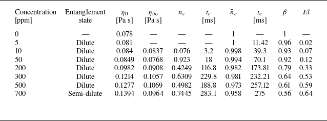


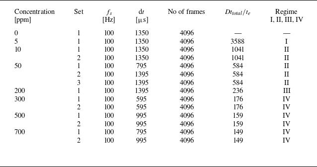

 Ωθ/Ωi
 Re
 Wi
 Wi
 Wi
 Wi
 Wi

 ur
 Wi

 ur,in¯
 ur,out¯
 Wi
 Ωiri
 R=ur,in¯/ur,out¯
 Wi
 |Ωθ|
 |Ωθ,rms′|
 Ωi

 Af
 Wi

 Cur′ (ξ)
 Cuz′ (ξ)
 Wi

 Cur′ (ξz)
 Wi
 −2⩽ξz/d⩽2

 tint
 Wi
 Cur′ (τ)
 tint
 Ωi
 te
 Wi

 Wi
 te
 −5/3
 −3
 f=0.2/te
 Wi
 Wi
 Wi
 Wi
 −5/3
 −3

 δur/Ωiri
 ξz/d
 Kurtosis
 ξz/d
 Wi

 S2(ξ)=<[δur(ξ)]2>
 Wi
 ξ/d
 S2(ξ)
 (ξ/d)2

 Kurtosis
 τ/te
 τ/te≈
 K
 Wi

 τrz′=|ur′uz′|
 mm2s−2
 K=(ur′)2+(uz′)2/3
 mms−1
 Wi
 Q⩾
 s−2

 τrz,G′ (mm2s−2)
 KG (mms−1)
 Wi

 K
 Wi
 K
 D=d
 K
 Wi
 Wi
 Q⩾
 s−2
 Kcr

 τrz′
 τrz′>τrz,cr′
 τrz′<τrz,cr′
 ta
 th
 Wi
 S
 Tcycle=ta+th
 tint
 te
 Wi
 Wi

 Wi

 ur,in¯
 ur,out¯
 Wi
 max(ur,rms′)
 |Ωθ|
 |Ωθ,rms′|

 ur,filt
 Wi

 Ωθ
 Wi

 ta
 th
 Wi
 S
 Kcr

 ta
 th
 Wi
 S
 D

 Kcr
 D
 Tcycle/te
 tint/te

 Open access

