1. Introduction
Cities are the central focus of global decarbonization initiatives, considering their major contribution (>70%) to the CO2 emissions from fossil fuels. They contribute significantly to global climate change through extensive emissions and are also highly vulnerable to its negative consequences, as they house more than half of the world’s population (U. N. Report 2019a). Accurately monitoring these emissions is of paramount importance for effective mitigation policies (Wang et al. Reference Wang, Zhou, Niu, Xiong, Wu, Cheng, Hou, Lu and Du2021). Furthermore, estimating fossil fuel CO2 emissions in cities involves two primary methods: the bottom-up and top-down approaches. The bottom-up method utilizes available data from fuel use and emission activities, but it carries significant uncertainty when applied to spatial scales of cities and urban areas (Andres et al. Reference Andres, Boden, Bréon, Ciais, Davis, Erickson, Gregg, Jacobson, Marland, Miller, Oda, Olivier, Raupach, Rayner and Treanton2012; Marland et al. Reference Marland, Boden and Andres2003). This uncertainty mainly comes from the difficulty in accurately quantifying fuel-use statistics at fine spatial and temporal resolutions. In addition, emission factors can also vary across locations, even for the same fuel type, which further increases the uncertainty (Wang et al. Reference Wang, Zhou, Niu, Xiong, Wu, Cheng, Hou, Lu and Du2021). In contrast, the top-down approach uses atmospheric CO2 concentration measurements from a network of sites for estimations (Miller et al. Reference Miller, Lehman, Verhulst, Miller, Duren, Yadav, Newman and Sloop2020). However, measuring CO2 concentrations alone cannot distinguish the contributions of fossil fuel CO2 fluxes from other sources, as mole fraction observations cannot inherently distinguish between fossil and biogenic contributions when they co-occur within the same region (Miller et al. Reference Miller, Lehman, Verhulst, Miller, Duren, Yadav, Newman and Sloop2020; Turnbull et al. Reference Turnbull, Graven, Krakauer, Schuur, Druffel and Trumbore2016). Similarly, the approach of using the difference between urban and background CO2 concentrations is not a direct method to estimate CO2ff, since the observed enhancement often reflects a mixture of signals from fossil fuel emissions as well as biospheric fluxes. To overcome this, an independent approach based on radiocarbon as a tracer can be employed (Levin et al. Reference Levin, Kromer, Schmidt and Sartorius2003). Radiocarbon-based source apportionment exploits the contrast between radiocarbon-free fossil-fuel CO2 and modern atmospheric CO2. Because fossil fuels are millions of years old, their 14C has completely decayed (half-life= 5730 years), and their combustion dilutes the atmospheric 14C/12C ratio—an effect known as the Suess effect (Suess Reference Suess1955). This principle is widely used to quantify fossil-fuel CO2 in polluted air (Niu et al. Reference Niu, Zhou, Wu, Cheng, Lu, Xiong, Du, Fu and Wang2016; Riley et al. Reference Riley, Hsueh, Randerson, Fischer, Hatch, Pataki, Wang and Goulden2008; Santos et al. Reference Santos, Oliveira, Park, Sena, Chiquetto, Macario and Grainger2019; Sharma et al. Reference Sharma, Kunchala, Ojha, Kumar, Gargari and Chopra2023a, Reference Sharma, Kunchala, Ojha, Kumar, Khandelwal, Gargari and Chopra2023b; Varga et al. Reference Varga, Barnucz, Major, Lisztes-Szabó, Jull, László, Pénzes and Molnár2019; Vay et al. Reference Vay, Tyler, Choi, Blake, Blake, Sachse, Diskin and Singh2009; Wang et al. Reference Wang, Zhou, Niu, Xiong, Wu, Cheng, Hou, Lu and Du2021; Zhou et al. Reference Zhou, Niu, Wu, Xiong, Hou, Wang, Feng, Cheng, Du, Lu, An, Burr and Zhu2020). Radiocarbon observations detect recently added fossil fuel CO2 (CO2ff) in the atmosphere which represents the net increase in the atmospheric fossil CO2 based on the comprehensive assessment of CO2 fluxes from various sources and sinks, including terrestrial biosphere (photosynthesis, respiration, biomass burning), oceans and nuclear emissions.
In recent decades, due to more substantial economic growth and increasing urbanization, India, the third highest emitter, has contributed 7% of the world’s fossil fuel CO2 emissions in 2021 (Crippa et al. Reference Crippa, Guizzardi, Banja, Solazzo, Muntean and Schaaf2022). As of 2018, India has the second-largest urban population in the world, after China (837 million), with a projected increase to 879 million (53% of the total population) by 2050 (U. N. Report 2019b). In 2018, India had five megacities (cities with a population exceeding 10 million): Delhi, Mumbai, Kolkata, Chennai, and Bangalore. Two additional cities, Ahmedabad and Hyderabad, are expected to become megacities by 2030. Given this rapid rate of urbanization, understanding fossil fuel emissions from Indian cities is essential for planning future low-carbon cities and fulfilling commitments under the Paris Agreement (Tong et al. Reference Tong, Nagpure and Ramaswami2021). To address these issues, it is vital to determine the contribution of urban fossil fuel CO2 emissions. Radiocarbon-based observations of fossil fuel CO2 (CO2ff) can provide an accurate estimate of such emissions from Indian cities.
In light of the aforementioned context, we analyzed variations in CO2ff in the megacity Delhi using radiocarbon measurements obtained during a multiyear campaign spanning from 2018 to 2022. These radiocarbon measurements were further used to investigate annual and seasonal variations of CO2ff over the study region. Additionally, we determined emission ratios RCO and RNOx for Delhi, and investigated the impact of COVID-19 lockdowns on CO2ff observations.
2. Material and methods
2.1. Study area
Delhi, the capital city of India, is situated in the northern part of the country between latitudes of 28.45°N – 28.85°N and longitudes of 76.50°E and 77.20°E at altitude of 227 m above the mean sea level (Chaurasia and Mohan Reference Chaurasia and Mohan2022). According to the 2011 census, Delhi is a densely populated city with a population density of 11,297 persons/km2, covering a geographical area of 1484 km2. It is the second-largest megacity in the world, following Tokyo, and is projected to become the largest megacity in the world in 2028 (U. N. Report 2019b). Delhi is a landlocked city surrounded by cities from the Haryana, Uttar Pradesh, and Rajasthan states. It is situated in the Indo-Gangetic Plain, which is connected to the Himalayas in the north and the Thar deserts in the west of Rajasthan. Due to its geographical location, Delhi experiences four distinct seasons: summer (April–June), monsoon (July–September), post-monsoon (October–November), and winter (December–March) (Perrino et al. Reference Perrino, Tiwari, Catrambone, Dalla Torre, Rantica and Canepari2011). Summers in Delhi are scorching with maximum temperatures reaching up to 48 °C (Jain et al. Reference Jain, Tripathi, Tripathi, Sahu, Gaddamidi, Shukla, Bhattu and Ganguly2022). The majority of Delhi’s rainfall, approximately 80%, occurs during the southwest monsoon season, which brings an average annual rainfall of 670 mm (Yadav et al. Reference Yadav, Mishra and Gurjar2022). In contrast, winters in Delhi are very cold, with a minimum temperature of up to 2°C. The city also receives some rainfall during winter due to western disturbances (Guttikunda et al. Reference Guttikunda, Dammalapati, Pradhan, Krishna, Jethva and Jawahar2023). Delhi had a total of 14 million registered vehicles, in addition to vehicles commuting to and from nearby satellite cities such as Noida, Gurugram, Faridabad, Ghaziabad, Sonipat, and others (Guttikunda et al. Reference Guttikunda, Dammalapati, Pradhan, Krishna, Jethva and Jawahar2023). Delhi is home to numerous small and large industrial units and has three gas-fired thermal power plants. Two coal-fired power plants (Rajghat and Badarpur) closed their operations in 2015 and 2018, respectively.
2.2. Sampling site and sample collection
We collected samples on the rooftop (20 m height) of the Inter-University Accelerator Centre (IUAC) building in New Delhi, specifically at the location of the Accelerator Mass Spectrometry (AMS) facility. IUAC is situated in the southwest part of Delhi, in an institutional cum residential area, as depicted in Figure S1. The nearest local fossil fuel pollution source is a road located approximately 150 meters away from the sampling location. We placed 80 mL of carbonate-free 2M sodium hydroxide solution in a 600 mL glass beaker (Duron make) for one week to collect the samples. This beaker was kept on a stand of 30 cm height over the rooftop under the shelter of a solar panel to protect it from rainwater and water vapor condensation during nighttime. There will still be some water vapor condensation, but it will not be enough to affect the capacity of the sample solution. The atmospheric CO2 was precipitated in the form of carbonate in this sampling method. Occasionally, due to uncontrollable factors such as high winds, rain, or holidays, samples were collected for a duration shorter or longer than one week. The carbonate samples were carefully stored in airtight vials until the radiocarbon measurement.
2.3. Sample graphitization
The CO2 obtained from the carbonate samples was converted into graphite for 14C-AMS measurements. This conversion process is known as graphitization and is carried out using an automated graphitization equipment (AGE3 from IonPlus AG, Switzerland) interfaced with a carbonate handling system (CHS from IonPlus AG, Switzerland) in the graphitization laboratory of the IUAC – AMS facility (Sharma et al. Reference Sharma, Umapathy, Kumar, Ojha, Gargari, Joshi, Chopra and Kanjilal2019). Carbonate samples were taken in 4.5 mL glass septum vials (Labco exetainer) and air in the vials was flushed with helium (He) gas at a flow rate of 80 mL/min for 5 min. Subsequently, samples underwent acid hydrolysis with 1 mL H3PO4 acid, and CO2 was transported into the zeolite trap of AGE with helium gas as a carrier. The trapped CO2 was later transferred into tubes filled with iron powder, using thermal expansion, where it was reduced by hydrogen into graphite over the surface of iron powder at 580°C temperature.
2.4. Radiocarbon measurements
Radiocarbon in the graphite samples were measured using a 500 kV Pelletron-based accelerator mass spectrometer at the IUAC AMS facility (Sharma et al. Reference Sharma, Umapathy, Kumar, Ojha, Gargari, Joshi, Chopra and Kanjilal2019). Unknown samples along with primary standard samples (OXII), background samples (IAEA C1) and secondary standard samples (IAEA C2 and C3) were loaded into the cathode wheel of the ion source of the accelerator, and radiocarbon was measured in the form of 14C/12C ratio. Online AMS δ13C values were used for the isotopic fractionation correction. 14C/12C ratio of these samples is converted into Δ14C as per the following relation
 ${\Delta ^{14}}C = \left[ {{{{{\left( {{{^{14}C} \over {^{12}C}}} \right)}_{SN}}} \over {{{\left( {{{^{14}C} \over {^{12}C}}} \right)}_{\rm abs}}}} - 1} \right] \times 1000\%$
where (14C/12C)SN is the measured 14C/12C ratio in the samples. This ratio is normalized with δ13C value of −25‰ for isotopic fractionation correction. (14C/12C)abs is the absolute ratio of the radiocarbon reference sample. This ratio is corrected for isotopic fractionation as well as radiocarbon decay (Stuiver and Polach Reference Stuiver and Polach1977). Uncertainties in Δ14C values are the same as the radiocarbon measurement precision of the sample. Uncertainties for individual samples vary from 1.5‰ to 3.4‰. Δ14C values of all the samples along with their uncertainties are given in Table S1.
2.5. CO2ff calculation
Δ14C values are converted into fossil fuel CO2 (CO2ff) values using the following mass balance equations (Turnbull et al. Reference Turnbull, Rayner, Miller, Naegler, Ciais and Cozic2009)
 ${\rm{C}}{{\rm{O}}_{{\rm{2mes}}}} = {\rm{C}}{{\rm{O}}_{{\rm{2bg}}}} + {\rm{C}}{{\rm{O}}_{{\rm{2ff}}}} + {\rm{C}}{{\rm{O}}_{{\rm{2oth}}}}$
 ${\Delta ^{{\rm{14}}}}{{\rm{C}}_{{\rm{mes}}}}{\rm{C}}{{\rm{O}}_{{\rm{2mes}}}} = {\Delta ^{{\rm{14}}}}{{\rm{C}}_{{\rm{bg}}}}{\rm{C}}{{\rm{O}}_{{\rm{2bg}}}} + {\Delta ^{{\rm{14}}}}{{\rm{C}}_{{\rm{ff}}}}{\rm{C}}{{\rm{O}}_{{\rm{2ff}}}} + {\Delta ^{{\rm{14}}}}{{\rm{C}}_{{\rm{oth}}}}{\rm{C}}{{\rm{O}}_{{\rm{2oth}}}}$
Where CO2bg = CO2 mole fraction at background site
CO2mes = CO2 measured at sampling location
CO2ff = fossil fuel CO2 at sampling location
CO2oth = CO2 from other sources such as the ocean, heterotopic respiration, etc.
Δ14Cmes = Δ14C measured in the atmospheric CO2 samples collected in the form of carbonate
Δ14Cbg = Δ14C value of background sample
Δ14Cff = Δ14C value of CO2 from fossil fuels. Since 14C is zero in fossil fuels.
Therefore, Δ14Cff = –1000‰ as per the definition of Δ14C (see eq. 5.1).
Δ14Coth = Δ14C value from other sources such as the ocean, nuclear emissions, heterotopic respiration, etc.
After solving equations (2) and (3) for CO2ff, we get the following expression
 ${\rm{C}}{{\rm{O}}_{2{\rm{ff}}}} = {\rm{\;}}{{{{\rm{C}}{{\rm{O}}_{2{\rm{bg}}}}{\rm{\;}}\left( {{\Delta ^{14}}{{\rm{C}}_{{\rm{mes}}}} - {\rm{\;}}{\Delta ^{14}}{{\rm{C}}_{{\rm{bg}}}}} \right)}}\over{{{\Delta ^{14}}{{\rm{C}}_{{\rm{ff}}}} - {\rm{\;}}{\Delta ^{14}}{{\rm{C}}_{{\rm{mes}}}}}}} - {\rm{\;}}{{{{\rm{C}}{{\rm{O}}_{2{\rm{oth}}}}{\rm{\;}}\left( {{\Delta ^{14}}{{\rm{C}}_{{\rm{other}}}} - {\rm{\;}}{\Delta ^{14}}{{\rm{C}}_{{\rm{mes}}}}} \right)}}\over{{{\Delta ^{14}}{{\rm{C}}_{{\rm{ff}}}} - {\rm{\;}}{\Delta ^{14}}{{\rm{C}}_{{\rm{mes}}}}}}}$
The second term in the above CO2ff expression represents the contributions from other sources. The contribution from oceanic sources can be neglected because Delhi is located far from the ocean, and the large-scale oceanic exchange has a similar effect on both the background and the sampling locations. It is also reported that the radiocarbon emissions from nuclear power plants also affect radiocarbon observations (Varga et al. Reference Varga, Orsovszki, Major, Veres, Bujtás, Végh, Manga, Jull, Palcsu and Molnár2020a). The nearest nuclear power plant from the sampling location is located at a distance of approx. 150 KM. Therefore, contributions from nuclear emissions can also be neglected. Heterotopic respiration is the only remaining contributor to this term and ignorance of it will induce an error of 0.4 – 0.8 ppm in summer and 0.2 – 0.3 ppm in winter in CO2ff values as reported by Turnbull et al. (Reference Turnbull, Rayner, Miller, Naegler, Ciais and Cozic2009). As per this study, this bias is generally consistent across most of the Northern Hemisphere land regions (including subtropical areas). We have also assumed no effect from autotrophic respiration, as its short residence time (<1 year) leads to Δ14C values that closely reflect the contemporary atmosphere. CO2ff values for all the samples along with their uncertainties are given in Table S1.
2.6. Background selection
Unfortunately, we do not have Δ14Cbg and CO2bg data from an Indian site for the study period from November 2018 to December 2022. For Δ14Cbg, in this case, the ideal approach would be to utilize Δ14C values of NH Zone 3 (Hua et al. Reference Hua, Turnbull, Santos, Rakowski, Ancapichún, De Pol-Holz, Hammer, Lehman, Levin, Miller, Palmer and Turney2022) since our study location falls in this zone. However, the available data from this source is only up to May 2019. We obtained monthly Δ14C data from another background site, Point Barrow, Alaska, USA (71.3°N, 156.6°W) from Dr. Xiaomei Xu, UCI, Irvine and this dataset is available up to August 2022. This dataset covers most of our study period, except for the last four months, from September 2022 to December 2022. To fill this gap, we have extrapolated this data based on the trend in Δ14C values for individual months from 2017–2021. We also utilized the monthly CO2 values for the background from the Point Barrow site as CO2bg values for our study (Keeling et al. Reference Keeling, Piper, Bacastow, Wahlen, Whorf, Heimann, Meijer, Ehleringer, Cerling and Dearing2005). We understand that choosing a background site outside of India introduces a latitudinal gradient in Δ14C and CO2 values, which may introduce some bias in our results. To assess this bias, we performed a sensitivity test and found that a change of 5 ppm in CO2bg value can induce a maximum difference of 0.5 ppm in our CO2ff observations. Similarly, a change of 2‰ in Δ14Cbg can cause a maximum change of 0.9 ppm in our observations. We have included these uncertainties in calculating final CO2ff uncertainties and reported them in Table S1.
2.7. Data used in this study
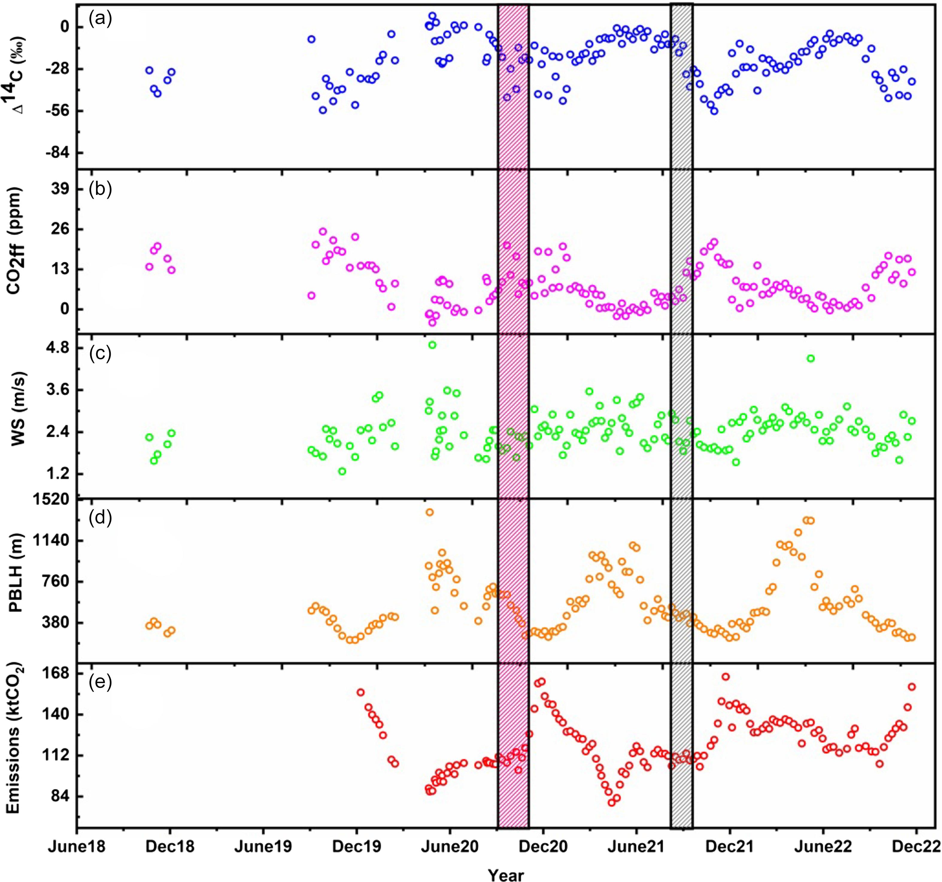
We obtained daily Planetary Boundary Layer Height (PBLH) and wind speed data from the ECMWF Reanalysis v5 (ERA5) dataset for our sampling location. The pollutant concentration data from the Sri Arvindo Marg site was downloaded from https://app.cpcbccr.com/ccr/#/caaqm-dashboard/caaqm-landing website. Near real-time daily fossil fuel CO2 emission data (ktCO2 per day) for Delhi is downloaded from 2019 to 2022 from the Carbon Monitor project (https://cities.carbonmonitor.org/). We calculated the average of available daily data for the period of each sample in our study (see Figure 1e).
Time series of (a) Δ14C, (b) CO2ff, (c) wind speed (WS), (d) PBLH in megacity Delhi from November 2018 to December 2022. Fossil fuel emissions of Delhi city from January 2020 to December 2022 are plotted in panel (e). Pink and gray shaded areas show the first and second COVID-19 waves.

Figure 1 Long description
Panel A: A scatter plot shows the time series of delta 14C (percent) from November 2018 to December 2022. The x-axis represents the year, and the y-axis represents delta 14C values. The data points are plotted in blue. Panel B: A scatter plot shows the time series of CO2ff (parts per million) over the same period. The x-axis represents the year, and the y-axis represents CO2ff values. The data points are plotted in pink. Panel C: A scatter plot shows the time series of wind speed (WS) in meters per second. The x-axis represents the year, and the y-axis represents WS values. The data points are plotted in green. Panel D: A scatter plot shows the time series of planetary boundary layer height (PBLH) in meters. The x-axis represents the year, and the y-axis represents PBLH values. The data points are plotted in orange. Panel E: A scatter plot shows the time series of fossil fuel emissions in kilotons of CO2. The x-axis represents the year, and the y-axis represents emissions values. The data points are plotted in red. Pink and gray shaded areas indicate the first and second COVID-19 waves.
2.8. Footprint analysis
We utilized the footprints method to differentiate between various source regions influencing each sample at the receptor location. These footprints were calculated using the FLEXCPP, developed by the Center for Global Environmental Research (CGER), Earth System Division (ESD), National Institute for Environmental Studies (NIES), Japan. FLEXCPP is a Lagrangian particle dispersion program based on FLEXPART (Flexible Particle Dispersion Model), utilizing meteorological data from the National Centre for Environmental Prediction (NCEP) (Saha et al. Reference Saha, Moorthi, Wu, Wang, Nadiga and Tripp2011). The backward run of FLEXCPP was conducted with a 1° grid resolution at a height of 100 m for the collection period of each sample, typically spanning 7 days, to determine the footprint. The footprints calculated in this manner depict the spatial pattern of emission sensitivities in each grid cell, reflecting the proportional residence time of particles in that specific grid cell.
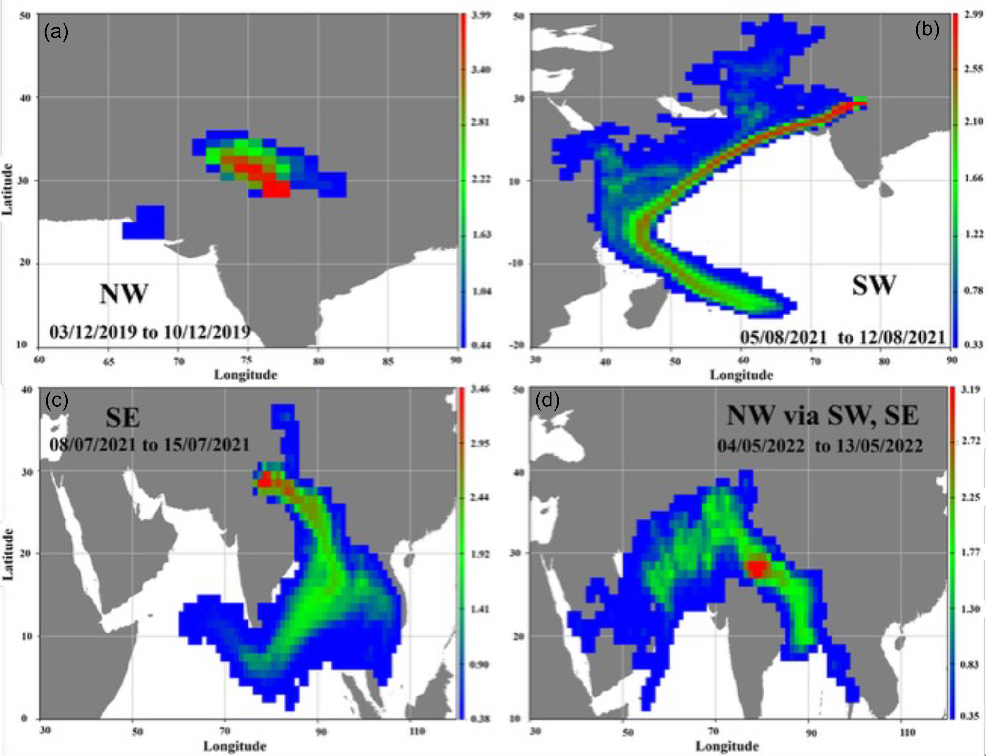
We manually screened footprints to identify the source regions for all samples in this study, revealing three predominant directions of distribution: northwest (NW), southwest (SW), and southeast (SE). Figure 2 (a–d) illustrates examples of footprints corresponding to each direction. NW is the prevailing wind direction in 63 of the 83 samples during winter and post-monsoon seasons. Among these, 44 samples face NW winds exclusively, while 19 samples experience winds from mixed directions, incorporating NW as one component (e.g., NW-SW, NW-West, etc.). Sources in the NW direction are primarily continental, dominated by local sources extending from nearby states to Pakistan and Afghanistan.
Representative examples of footprints for corresponding wind direction (a), Northwest (NW), (b) Southwest (SW), (c) Southeast (SE), (d) Mixed, NW via SW, SE. Details of footprint analysis are given in Method section 2.8.

Conversely, SW and SE are the predominant wind directions during the summer and monsoon seasons. Air from these directions originates mainly from the ocean, reaching Delhi either from the Indian Ocean or the Arabian Sea in the SW direction. For the SE direction, air travels to Delhi from the Bay of Bengal via the Indo Gangetic Plain (IGP) or from the Arabian Sea via the Bay of Bengal and IGP.
2.9. RCO and RNOx determination
Atmospheric radiocarbon observations at hourly scale are not possible at present due to laborious sample preparation, complex instrumentation and associated high cost of measurements. Therefore, it is difficult to observe CO2ff at high temporal resolutions such as hourly scale. However, CO and NOx can be used as a proxy for this purpose by determining emission ratios, i.e. RCO and RNOx. CO and NOx measurements are relatively less complex and available at hourly scale due to widespread networks of air quality stations. Lopez et al. (Reference Lopez, Schmidt, Delmotte, Colomb, Gros, Janssen, Lehman, Mondelain, Perrussel, Ramonet, Xueref-Remy and Bousquet2013) utilized these emission ratios (RCO and RNOx both) to determine continuous fossil fuel CO2 values in Paris city. Similarly, RCO is also utilized in Heidelberg city for determining the continuous record of fossil fuel CO2 (Maier et al. Reference Maier, Levin, Conil, Gachkivskyi, Denier van der Gon and Hammer2024). Here, we have also determined emission ratios RCO and RNOx for Delhi to assess their use as a proxy for CO2ff.
RCO and RNOx are defined below (Lopez et al. Reference Lopez, Schmidt, Delmotte, Colomb, Gros, Janssen, Lehman, Mondelain, Perrussel, Ramonet, Xueref-Remy and Bousquet2013):
 ${{\rm{R}}_{{\rm{CO}}}} = {\rm{C}}{{\rm{O}}_{{\rm{enh}}}}{\rm{/C}}{{\rm{O}}_{{\rm{2ff}}}} = \left( {{\rm{CO - C}}{{\rm{O}}_{{\rm{bg}}}}} \right){\rm{/C}}{{\rm{O}}_{{\rm{2ff}}}}$
 ${{\rm{R}}_{{\rm{NOx}}}} = {\rm{NOx/C}}{{\rm{O}}_{{\rm{2ff}}}}$
COenh is the enhanced CO concentration at the measurement site and is calculated after subtracting background CO concentrations (CObg) from the measured CO values. To maintain continuity, we have taken monthly averaged CO values from the point barrow site as CObg and subtracted them from the monthly average of measured CO values from Sri Aurobindo Marg station, Delhi. We have also examined the sensitivity of the RCO value to the background CO values. We re-evaluated the RCO values after excluding background CO. Similar to a study in Paris by Lopez et al. (Reference Lopez, Schmidt, Delmotte, Colomb, Gros, Janssen, Lehman, Mondelain, Perrussel, Ramonet, Xueref-Remy and Bousquet2013), we did not use background value for NOx because it has a very small lifetime (∼9 hr). CO2ff is regressed linearly with COenh and NOx, respectively, and slopes of the regression lines provide RCO and RNOx ratios. We have used York fit to determine the slope of regression lines using the bfsl (best fit straight line) package in R (Sturn Reference Sturm2018). The york fit considers the uncertainties of both dependent and independent variables during determining the slope of regression lines and is the preferred method to determine RCO in other studies (Maier et al. Reference Maier, Levin, Conil, Gachkivskyi, Denier van der Gon and Hammer2024; Young et. al. Reference Young, Turnbull, Keller, Domingues, Parry-Thompson, Hilton and Mikaloff-Fletcher2023).
3. Results
3.1. Annual and seasonal variations of fossil fuel CO2
The Δ14C and CO2ff values from 2018–2022 are illustrated in Figure 1 (a) and (b) and monthly average values are shown in the supplementary information (Figures S2 (a) and (b)). Δ14C and CO2ff values for all the samples along with their uncertainties are given in Table S1. Δ14C values range from –56.2‰ to 7.5‰, while CO2ff values vary from 25.2 ppm to a value close to zero ppm, respectively. The highest CO2ff value was observed in October 2019, while the lowest value was observed in May 2020. The corresponding fossil fraction (CO2ff expressed as a percentage of background CO2, following the description given in (Varga et al. Reference Varga, Jull, Lisztes-Szabó and Molnár2020b; Chakraborty et al. Reference Chakraborty, Dutta, Bhattacharyya, Nigam, Schuur and Shah2008) varies from 0.1 to 6.2% for the study period.
A clear seasonal trend in CO2ff values is observed, having higher values in post-monsoon (October–November) and winter (December–March) seasons and lower values in summer (April–June) and Monsoon (July–September) seasons as shown in Figure 1 (b) and also visible in the monthly averages presented in Figure S1 (b).
These seasonal CO2ff observations are well supported with the planetary boundary layer height (PBLH), wind speed data, and footprint analysis, as shown in Figures 1(e, f) and 2 (a–d), respectively. During the post-monsoon and winter seasons, the combination of low PBLH and low wind speed inhibits the dispersion of emissions, leading to a higher concentration of fossil fuel emissions trapped within the boundary layer. Footprint analysis also shows that samples are affected by continental polluted air from the Northwest direction and local sources dominate during these seasons (Figure 2a, see Method section 2.8). As a result, higher values of CO2ff are observed near to the surface. In contrast, during the summer and monsoon seasons, the PBLH increases due to higher temperatures, facilitating the mixing of surface-level fossil fuel CO2 emissions into the deeper atmospheric boundary layer. The higher wind speed in these seasons also aids in the ventilation of emissions (Metya et al. Reference Metya, Datye and Chakraborty2021). Prevailing wind directions in these seasons are either southwest or southeast which brings clean air from the Indian Ocean, Arabian Sea or Bay of Bengal (Figures 2b–d), resulting in lower CO2ff values.
We have plotted fossil fuel CO2 emissions from bottom-up inventory from Carbon Monitor for Delhi city along with our CO2ff observations as shown in Figure 1(e). Although a direct comparison between these two datasets is difficult, we have compared the seasonal trends. Total CO2 emissions from fossil fuels also peaked in winter, similar to CO2ff observations. However, fossil fuel emissions in winter and post-monsoon seasons were 14.4%, 9.5% and 2.2% higher than the summer and monsoon seasons in 2020, 2021 and 2022, respectively (see Figure S3). Since emissions in the summer season were affected in 2020 and 2021 due to COVID-19 related restrictions, no such restrictions were observed in 2022. Therefore, the observed high CO2ff values in Delhi during the winter and post-monsoon season are primarily attributed to atmospheric stagnant conditions characterized by lower PBLH and lower wind speeds.
We have calculated annual averages for 2021 and 2022, as we have samples covering the entire two years. In 2021, the average value of Δ14C (mean ± SD) is −20.5 ± 15.4‰, while in 2022, it is –23.4 ± 11.8‰. Correspondingly, the average CO2ff value is slightly higher in 2021 (6.8 ± 6.7 ppm) compared to 2022 (6.6 ± 4.9 ppm). The Δ14C exhibits a decrease (3.3‰) at the background site compared to Delhi city (2.9‰) between 2021 and 2022, leading to a slightly lower CO2ff value in 2022. Additionally, policy decisions, such as the ban on coal usage in industrial activities in Delhi-NCR from October 2022 in the areas where pressurized natural gas (PNG) supply infrastructure is available (except in thermal power plants) and the initiation of co-firing of biomass in 11 TPPs within a 300 km radius of Delhi-NCR in 2022, have played a significant role. Although biomass co-firing constitutes less than 1% of total coal use in these plants, it has slightly improved air quality in 2022 (CEA annual report 2022–2023).
In addition to the annual averages, we have five-to-six-year data of CO2ff for specific months, as shown in Figure S2(b). For example, in November, CO2ff values vary between 10.5 ppm to 18.8 ppm in the study period. Similarly, in October, the CO2ff values were higher in 2019, with value of 16.9 ppm, while they remain relatively constant (10.2 ppm, 10.5 ppm, and 10.5 ppm) from 2020 to 2022. The value of CO2ff is somewhat lower (10.4 ppm) in December 2020, while it is higher in other years, as depicted in Figure S2(b). The CO2ff values in 2020 were affected by COVID-19 restrictions. It is important to note that thermal power plants (electricity consumption) are the highest contributor (52%) to the CO2 emissions in Delhi, followed by vehicles (27%) (Nagar et al. Reference Nagar, Sharma, Gupta and Singh2019). However, in 2018, one coal-based power plant at Badarpur is closed and utilization of the other two units (Indraprastha CCPP, Pragati CCPP) is reduced, having annual power load factor (PLF) from 10% to 54% (Guttikunda et al. Reference Guttikunda, Dammalapati, Pradhan, Krishna, Jethva and Jawahar2023). Due to the power plant’s closure in 2018, emissions were reduced by 7.25% in 2018. The emissions increased by 2% in 2019, decreased in 2020 due to lockdown restrictions, and bounced back again in 2021 (Arora et al. Reference Arora, Reddy, Sharma, Kilaparthi and Gupta2023). Our observations were able to capture these variations in the local emissions and highest values of CO2ff in our study vary accordingly during 2018–2021.
3.2. Emission ratios (RCO and RNOx)
RCO and RNOx values for overall data (Nov. 2018 to Dec. 2022) and three seasons i.e., winters, post monsoon and summer, are shown in Table 1 with their coefficient of determinations (r2) and Figure S4 (a, b) and S5 (a, b) show the regression plots of CO and NOx, respectively using which emission ratios are determined. Ratios for the monsoon season are not reported because of their statistical insignificance.
RCO and RNOx values in Delhi.

Table 1 Long description
A table comparing RCO and RNOx values across different years and seasons. The table has four rows and five columns. The columns are labeled Years/seasons, RCO (ppb/ppm), r2, RNOX (ppb/ppm), and r2. The row labels are 2018-2022, Winters, Post-monsoon, and Summer. Row 1: 2018-2022, RCO (ppb/ppm) 39.0 ± 1.9, r2 0.31, RNOX (ppb/ppm) 2.1 ± 0.1, r2 0.52. Row 2: Winters, RCO (ppb/ppm) 37.5 ± 5.3, r2 0.13, RNOX (ppb/ppm) 1.6 ± 0.3, r2 0.37. Row 3: Post-monsoon, RCO (ppb/ppm) 39.60 ± 5.3, r2 0.14, RNOX (ppb/ppm) 2.2 ± 0.3, r2 0.35. Row 4: Summer, RCO (ppb/ppm) 38.7 ± 3.9, r2 0.06, RNOX (ppb/ppm) 2.0 ± 0.3, r2 0.10.
RCO value for all years (Nov. 2018 to Dec. 2022) data is 39.0 ± 1.9 ppb/ppm. RCO values in winter, post monsoon and summer seasons are also close to this value within their uncertainties. RNOx value is 2.1 ± 0.1 ppb/ppm in Delhi for all years (2018–2022) data while seasonal values are also nearby to each other within their uncertainties.
3.3. Effect of COVID-19 restrictions
India implemented nationwide COVID-19 lockdowns during March–May 2020, followed by a phased unlocking from 8 June 2020, which led to a marked reduction in anthropogenic activities and improved air quality in the Delhi–NCR region (Mahato et al. Reference Mahato, Pal and Ghosh2020; Sharma et al. Reference Sharma, Zhang, Gao, Zhang and Kota2020). Unfortunately, we could not collect samples during the first three phases (strictest phases) of the lockdown. Our sampling for this study commenced on May 20 during the fourth phase of the lockdown.
A second wave in April–June 2021 resulted in renewed restrictions in Delhi, though less stringent than in 2020, with several essential and transport services operating at limited capacity (Kolluru et al. Reference Kolluru, Nagendra and Patra2023). A full lockdown was announced on 19 April 2021, which was extended multiple times until 7 June 2021. The unlocking process began on 8 June 2021, with a gradual lifting of restrictions (Kolluru et al. Reference Kolluru, Nagendra and Patra2023). We collected samples during the second wave of COVID-19 in Delhi.
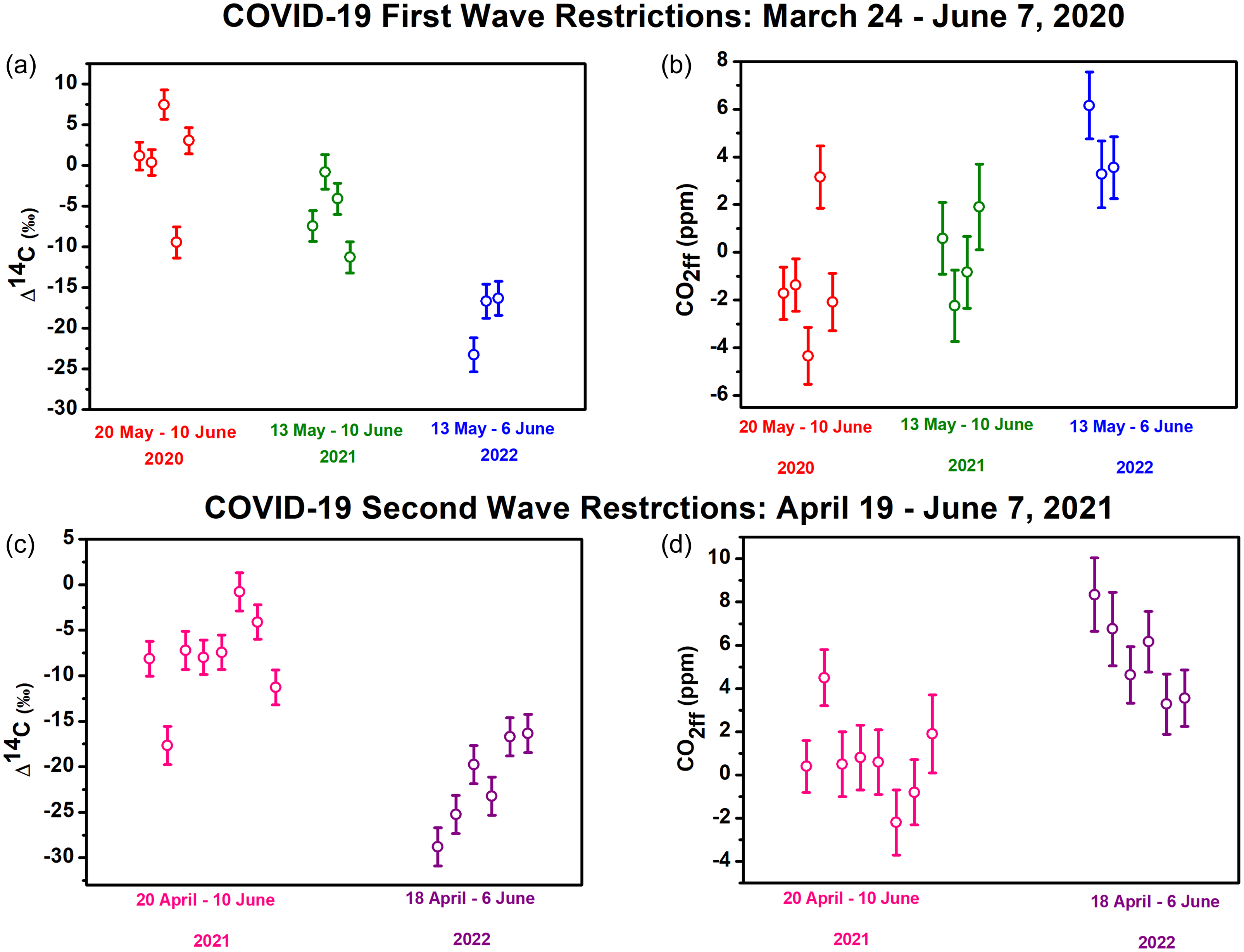
We first examined the impact of the complete lockdown during the first wave of COVID-19 pandemic on Δ14C and CO2ff values. To assess the comparison between two years, we compared the Δ14C and CO2ff values in Figure 3 (a) and (b), respectively, during the overlapping period of the lockdown, specifically from 20 May to 8 June in 2020, 2021, and 2022. As we do not have data from 2019 for the corresponding period, we compared the data from 2022 when there were no restrictions. An apparent decrease in Δ14C (Figure 3a) and an increase in CO2ff values (Figure 3b) is visible during this period from 2020 to 2022. The average values (±SD) of observed Δ14C during this period were 0.5 ± 5.7 ‰ in 2020, −5.9 ± 3.9 ‰ in 2021, and −18.8 ± 3.9 ‰ in 2022. The corresponding average values (±SD) of CO2ff were near zero in 2020 and 2021 and 4.3 ± 1.3 ppm in 2022. Notably, there was an increase of 1.1 ppm in 2021 and 5.6 ppm in 2022 compared to 2020.
Comparison of Δ14C and CO2ff values of samples collected during COVID-19 (a & b) first-wave restrictions and (c & d) second-wave restrictions with the same period in 2022 when there were no restrictions.

During the second wave, we found that Δ14C values are higher (Figure 3c) while CO2ff values are lower (Figure 3d) during the restriction period in 2021 than in 2022. The average value (±SD) of CO2ff in this period was about 0.7 ± 1.8 ppm in 2021 and 5.5 ± 1.8 ppm in 2022. Notably, there was an increase of 4.8 ppm in 2022 compared to the 2021 value.
4. Discussion
Seasonal variations in radiocarbon-based CO2ff observations are frequently observed in studies conducted in several northern hemisphere cities (Graven et al. Reference Graven, Fischer, Lueker, Jeong, Guilderson, Keeling and Bambha2018; Levin et al. Reference Levin, Hammer, Eichelmann and Vogel2011; Miller et al. Reference Miller, Lehman, Verhulst, Miller, Duren, Yadav, Newman and Sloop2020; Niu et al. Reference Niu, Zhou, Wu, Cheng, Lu, Xiong, Du, Fu and Wang2016b; Zhou et al. Reference Zhou, Wu, Huo, Xiong, Cheng, Lu and Niu2014, Reference Zhou, Niu, Wu, Xiong, Hou, Wang, Feng, Cheng, Du, Lu, An, Burr and Zhu2020). Levin et al. (Reference Levin, Hammer, Eichelmann and Vogel2011) showed the seasonal variations in CO2ff (below 10 ppm in summer and up to 40 ppm in winter) in the long-term observations from 1986 to 2008 in Heidelberg, Germany. This study linked the seasonality with the higher emissions and suppressed vertical mixing due to temperature inversion conditions in the winter. Miller et al. Reference Miller, Lehman, Verhulst, Miller, Duren, Yadav, Newman and Sloop2020 reported CO2ff variations from –1.3 ppm to 48.4 ppm in the Los Angeles megacity in 2015. Also, they found approximately similar average CO2ff values for winter (14.0 ± 12.7 ppm) and summer seasons (13.2 ± 6.9 ppm) but higher variability in winters due to trapping emissions within the boundary layer more often than in summer. They attributed this higher variability to the variations in wind speed and boundary layer height rather than the actual increase in the emissions because fossil fuel emissions were only 3% higher in winter.
Similarly, Graven et al. (Reference Graven, Fischer, Lueker, Jeong, Guilderson, Keeling and Bambha2018) also revealed a large CO2ff in winter months from multiple sites in their study from California State, USA during 2014–2015 due to seasonality in atmospheric transport. In another study by Niu et al. (Reference Niu, Zhou, Wu, Cheng, Lu, Xiong, Du, Fu and Wang2016), CO2ff is determined using atmospheric 14C measurements in two Chinese cities, i.e., Beijing and Xiamen for one year in 2014. The CO2ff values ranged from 1.6 ± 1.3 ppm to 152 ± 1.7 ppm for Beijing and 2.5 ± 1.1 ppm to 54.6 ± 1.7 ppm for Xiamen, with average values of 39.7 ± 36.1 ppm and 13.6 ± 12.3 ppm, respectively in both cities. They have observed seasonal variations in CO2ff having high values in the winter season in Beijing city and attributed to the increased use of fossil fuels in winter for heating and the poor atmospheric vertical mixing. However, no seasonal variation was found in Xiamen, because this city is a coastal city with a relatively warm winter. Zhou et al. (Reference Zhou, Wu, Huo, Xiong, Cheng, Lu and Niu2014) reported the CO2ff variations in another inland Chinese city, Xian, for 2012–2013 and found that CO2ff values varied between 20.2 ± 9.8 ppm and 57.8 ± 17.1 ppm with an average value of 34.2 ± 9.5 ppm. Xian City also has high CO2ff values in the winter (46.5 ± 8.7 ppm) compared to summer (26.6 ± 3.4 ppm) because of a higher use of fossil fuels for heating and poor atmospheric dilution. Zhou et al. (Reference Zhou, Niu, Wu, Xiong, Hou, Wang, Feng, Cheng, Du, Lu, An, Burr and Zhu2020) estimated the fossil fuel CO2 using multiyear radiocarbon measurements in fifteen Chinese cities and found higher CO2ff values in January and lower values in July.
In comparison to these studies, our study over the megacity Delhi observed lesser CO2ff values (maximum 25.23 ppm) but revealed significant seasonal variations. As described in section 3.1, total emissions were only 2.2% higher in the winter and post-monsoon than the summer and monsoon season, which means high CO2ff values in Delhi during the winter and post-monsoon season are primarily due to atmospheric stagnant conditions characterized by lower PBLH and lesser wind speeds. This observation is similar to megacity Los Angeles, but the differences in CO2ff values in different seasons are identical to those in Chinese cities. Additionally, CO2ff values in the summer season in Delhi are also affected due to crop residue burning in the surrounding states. The impact of the southwest monsoon winds on Δ14C values during the monsoon seasons in India can also not be neglected (Hua and Barbetti Reference Hua and Barbetti2007). During this season, the intertropical convergence zone (ITCZ) position is extended up to 30°N in India. The air in this region is a mixture of air coming from southwest monsoon winds and air from the northern hemisphere region. Hua and Barbetti (Reference Hua and Barbetti2007) reported that Δ14C values in the tree ring samples from Mandla (India, 23°N, 81°E) during the period of 1963–1967 were lower compared to other sites at similar latitudes due to the influence of air masses depleted in 14C coming from the southern hemisphere, which dilutes the 14C values at Mandla. From 1963 to 1967, Δ14C values were significantly higher in the northern hemisphere (NH) than the southern hemisphere (SH), mainly attributed to extensive nuclear bomb testing in the former region. This positive gradient of Δ14C between the northern and southern hemispheres persisted until the 1990s. However, in the 2000s, the gradient reversed, and Δ14C values in SH were 5‰ higher than in NH, which increased to 7‰ higher in 2019 (Zhang et al. Reference Zhang, Liu, Li, Li, Wei and Xu2021). Consequently, slightly enriched air masses in 14C originating from the southern hemisphere during the southwest monsoon season may also contribute to the increased 14C levels observed in Delhi.
RCO values in our study are higher than the reported values from other studies such as Paris (10.8 ppb/ppm, Lopez et al. Reference Lopez, Schmidt, Delmotte, Colomb, Gros, Janssen, Lehman, Mondelain, Perrussel, Ramonet, Xueref-Remy and Bousquet2013), UK (5.7 ppb/ppm; Wagner et al. 2019), Auckland (11±1 ppb/ppm, Young et al. Reference Young, Turnbull, Keller, Domingues, Parry-Thompson, Hilton and Mikaloff-Fletcher2023), US cities and regions (9 – 14 ppb/ppm, studies performed between 2004 to 2013; Turnbull et al. Reference Turnbull2015), and Chinese cities (Beijing, 30.4 ± 1.6 ppb/ppm, Xiamen, 29.6 ± 3.2 ppb/ppm; Niu et al. Reference Niu, Zhou and Feng2018). Our RCO value is lesser than the value of 47 ± 13 ppb/ppm from another Chinese city, Xian, in 2016 (Liu et al. Reference Liu, Niu, Feng, Zhou, Liang, Lyu, Wang, Lu, Liu and Turnbull2024) and from East Asia (Tae – Ahn Peninsula, Korea, 44 ± 3 ppb/ppm, Shangdianzi, China, 47 ± 2 ppb/ppm, Turnbull et al. Reference Turnbull, Tans, Lehman, Baker, Conway, Chung, Gregg, Miller, Southon and Zhou2011). High RCO values in Delhi reflect the higher CO emissions in South Asia relative to other countries (Dasari et al. Reference Dasari, Andersson, Popa, Rockmann, Holmstrand, Budhavant and Gustafsson2021). They also indicate poor combustion efficiency in the Delhi region compared to other countries. The primary sources of CO in Delhi are the transport sector, residential sector, crop residue burning, municipality solid waste (MSW) burning, aviation and industry (Sahu et al. Reference Sahu, Mangaraj and Beig2023). The residential sector also includes CO emissions from biomass burning (wood, cow dung) for cooking and heating used in urban slums and rural parts of the surrounding areas of Delhi (Beig et al. Reference Beig, Korhale, Rathod, Maji, Sahu, Dole, Latha and Murthy2021). Biomass is also utilized as a fuel by small, unorganized industries (Beig et al. Reference Beig, Korhale, Rathod, Maji, Sahu, Dole, Latha and Murthy2021). CO emissions from biomass burning also favor the high RCO values because no CO2ff is emitted in this combustion (Niu et al. Reference Niu, Zhou and Feng2018). The revised analysis after excluding background CO values yielded an RCO value of 42.7 ± 2.1 ppb/ppm with an r2 of 0.27 for the entire dataset (2018–2022). This value is marginally higher, with the slightly reduced r2, though within the uncertainty range, compared to the previous estimate of 39 ± 1.9 ppb/ppm. We acknowledge that the absence of local background CO data may have influenced our RCO estimates. RNOx ratios in Delhi are close to ratios observed in Paris for mixed wind (2.8 ppb/ppm) regime (Lopez et al. 2010). The main sources of NOx in Delhi are dominated by the transport sector, followed by industry and aviation sectors (Sahu et al. Reference Sahu, Mangaraj and Beig2023). In other similar studies, the coefficient of determinations (r2) for RCO and RNOx were better than 0.75 (Lopez et al. Reference Lopez, Schmidt, Delmotte, Colomb, Gros, Janssen, Lehman, Mondelain, Perrussel, Ramonet, Xueref-Remy and Bousquet2013; Maier et al. Reference Maier, Levin, Conil, Gachkivskyi, Denier van der Gon and Hammer2024). In our study, r2 values for RCO and RNOx are very less for Delhi due to complexity of sources. Therefore, we did not use them for determining fossil fuel CO2 values at hourly scale.
Our analysis reveals a decrease of 5.6 ppm during the 2020 lockdown, while a reduction of 4.8 ppm was observed during the 2021 lockdown. As expected, CO2ff values were at their minimum from 20 May 2020 to 7 June 2020, given that minimal industrial and transport activities were allowed during that time. However, during the second wave, restrictions were not as strict as in 2020, leading to a rise in local CO2ff emissions than the previous year. Generally, these months tend to exhibit lower values of CO2ff due to favorable meteorological conditions such as large mixing depths and higher wind speeds. However, the lockdown measures further contributed to reducing these values. It is worth noting that the lowest CO2ff value of our study in the sample collected from 27 May to 29 May 2020. In June 2020 (see Figure S2b), a relatively higher CO2ff value was observed. This increase can be attributed to the initiation of the unlocking process during this month with the resuming of the operations of the workplaces and various industries. Consequently, CO2ff emissions from transportation and industrial activities began to rise.
Our earlier study, Sharma et al. Reference Sharma, Kunchala, Ojha, Kumar, Khandelwal, Gargari and Chopra2023b, mapped fossil-fuel-derived CO2 (CO2ff) across megacity Delhi using radiocarbon (14C) measurements in Peepal (Ficus religiosa) tree leaves collected from diverse locations, including parks, university campuses, and residential areas. The results revealed a highly heterogeneous spatial distribution of CO2ff across the city, ranging from 1.63 to 33.34 ppm. However, since Peepal trees shed their leaves once a year (around March), the leaf-based method provides an integrated annual record of CO2ff and cannot be used to infer seasonal or temporal variability of CO2ff. In contrast, the sampling approach adopted in the present study allows investigation of both temporal and seasonal variations at a single site. In summary, the earlier study focused on spatial variations in CO2ff across multiple sites in Delhi during April 2016 to March 2017, whereas the present study emphasizes temporal and seasonal variations from a single location within the megacity for the period 2018 to 2022.
In this study, we used Δ14Cbg and CO2bg data from a background site geographically distant from our sampling location. We acknowledge that this may have influenced the CO2ff estimates. In future work, we plan to extend this study by conducting simultaneous measurements of 14C and CO2 at an upwind site of Delhi to better constrain the background contributions.
5. Summary and conclusions
Our measurements reveal varying Δ14C values ranging from −56.2‰ to 7.5‰ and CO2ff values ranging from 0.3 ppm to 25.2 ppm. We observed a distinct seasonality in Δ14C and CO2ff, with higher (lower) values during winter and post-monsoon (summer and monsoon) seasons. This is not due to differences in the emissions but due to atmospheric conditions. Seasonality of CO2ff is similar to other NH cities but differences in CO2ff values in different seasons are identical to those in Chinese cities. Our study also examines the impact of the COVID-19 lockdown periods on CO2ff and observed a notable decrease of 5.6 (4.8) ppm during the pandemic’s first (second) waves. We have determined emission ratios (RCO and RNOx) and found that they are larger than the other cities in the world except Chinese cities.
In summary, our study provides valuable insights into the temporal variations of Δ14C and CO2ff in Delhi. These findings enhance our understanding of CO2 emission changes and their relationship to environmental factors, facilitating the development of effective strategies to mitigate greenhouse gas emissions in megacities like Delhi.
Supplementary material
The supplementary material for this article can be found at https://doi.org/10.1017/RDC.2026.10223.
Acknowledgments
Authors are thankful to IUAC for extending AMS facility for 14C funded by Ministry of Earth Science (MoES), Govt. of India with reference numbers MoES/16/07/11(i)-RDEAS and MoES/P.O.(Seismic)8(09)-Geochron/2012. Authors are thankful to Dr. Xiaomei Xu, UCI, Irvine for providing radiocarbon observations data for the background site, Point Barrow, Alaska, USA. We also acknowledge Haiden A Young, the lead author of the study in Young et al. (Reference Young, Turnbull, Keller, Domingues, Parry-Thompson, Hilton and Mikaloff-Fletcher2023), for providing codes in R to calculate the coefficient of determination (r2) values in bfsl package for York fit. Authors also acknowledge the help of Dr. Meenakshi in sample collection during COVID second wave.