

1 Introduction
Recent empirical findings shed doubt on the exclusively monotonic link between ability (as measured by income or wealth) and life expectancy. Though they do not explicitly explain it, von Gaudecker and Scholz (Reference Von Gaudecker and Scholz2007) and Kibele (Reference Kibele2008) discover a U-shaped relationship, whereas Hupfeld (Reference Hupfeld2008) specifically addresses the downward sloping part of the non-monotonic link.
I show that there exists a government (principal) objective and following effort levels of agents which are consistent with empirical findings, despite the fact that the respective objective (maximization of output from labor) is not necessarily desirable. In my model, an agent is capable of engaging in three different activities, one of which is concerned with investments in longevity (work out), and the others being weekly or instantaneous labor supply (work) and life-time labor supply (retirement). However, effort levels are not perfectly observable, such that the government (the principal) can only condition taxes (or subsidies) on perturbed signals. The principal (or the government) can levy taxes on certain observable phenomena, e.g. on work. These taxes (which may be negative) shift the revenue or outcome from activities between the agent and the principal, and at the same time allocate risk associated with this activity. The government is not strictly benevolent; it has own interests instead, which can be interpreted as the maximization of GDP, measured by output from work and length of the working life of the agent. However, although longevity is not valued in its own right by the principal, it is always indirectly considered in the tax system due to the interaction with work and retirement. Since the observation of the agent's effort levels is distorted, only a second-best solution is feasible. I apply the solution mechanism for multi-task moral-hazard situations proposed by Holmstrom and Milgrom (Reference Holmstrom and Milgrom1991), and derive comparative statics of the optimal incentives with respect to the agent's ability.
Several questions in this essay have already been addressed separately in different settings, but not together: Wolfe (Reference Wolfe1983) models an agent who has two choices, namely retirement age and consumption of leisure, which resembles the activities work and retirement in my specification. However, both activities are assumed to be perfectly observable, such that no moral hazard can arise. Instead, Wolfe finds adverse selection, since the agent chooses her retirement age (early or postponed) based on her life expectancy, which is not observed by the principal of the pension system. Individuals with high life expectancy benefit from a pension system that is actuarially fair for the average pensioner only. A similar reasoning is applied by Diamond (Reference Diamond2003), who shows that agents above a certain threshold of life expectancy or productivity can exploit the tax/pension system, because the principal has to keep incentives for agents with more intermediate characteristics. Also in an approach applying optimal taxation, Cremer et al. (Reference Cremer, Lozachmeur and Pestieau2004) analyze the interaction of health and productivity with respect to the resulting optimal tax scheme and find that delayed retirement is (relatively) taxed in order to subsidize the respective ‘weaker’ type, in order to enable him to retire earlier. Late retirement in their setting is still preferred by individuals with high productivity or good health, which are assumed to be positively correlated. Here, life expectancy is still exogenous (and equal across all types of individuals), and retirement age is assumed to by fully observable.
Introducing moral hazard, Davies and Kuhn (Reference Davies and Kuhn1992) endogenize life expectancy by the explicit modelling of longevity-enhancing behaviour; however, as opposed to the models of optimal taxation and in contrast to the model I present, income is assumed to be exogenous. The possible trade-off between consumption and investments in longevity is derived from the budget constraint and the utility decreasing or increasing effect of the investment. The authors find moral hazard, namely excessive investments in longevity, inflicting damage on private providers of annuities who, however, do not cease to exist, despite moral hazard.Footnote 1 Under the presence of private or public old-age annuities, Philipson and Becker (Reference Philipson and Becker1998) find a similar moral-hazard effect, where longevity is also endogenous. The authors additionally track the interaction with public health insurance, which potentially accelerates the moral-hazard effect, as no market prices govern the scarcity of longevity-enhancing means. In the following analysis, incentives for work out can be interpreted as a public health system.
Endogenized life expectancy relates to Grossman (Reference Grossman1972, Reference Grossman, Culyer and Newhouse2000), where investments in health capital consume time and mitigate instantaneous consumption, but allow higher productivity in the future and potentially delay the time at which the stock of health capital will be consumed. See additionally Wolfe (Reference Wolfe1985) for a treatment of this topic, who takes retirement explicitly into account as a special means of investment in one's health capital. Yet, in his setting, he fixes life expectancy, leaving an open issue to analyze. The main contribution of Ehrlich and Chuma (Reference Ehrlich and Chuma1990) is the explicit discrimination of the demand for health from the demand for longevity, the latter being directly dependent on the stock of health capital in Grossman (Reference Grossman1972, Reference Grossman, Culyer and Newhouse2000). My analysis differs in one main aspect from Grossman (Reference Grossman1972, Reference Grossman, Culyer and Newhouse2000) or Ehrlich and Chuma (Reference Ehrlich and Chuma1990), since I neither apply the notion of health capital, nor use any initial endowments in capital, health-related or physical.
The essay is organized as follows. Section 2 briefly reviews the relevant empirical literature. In the following, Section 3, I present the model, namely the interests of the agent and the principal, the technology that transforms inputs of the agent into output for the principal, the perturbations, and the tax system (the incentives). In Section 4, I solve the model and present comparative statics of the incentives with respect to a variation of the exogenous parameters, whereas Section 5 concludes and gives an outlook on further possibilities to enhance the presented model.
2 Empirical evidence
Overview: the relationship between life expectancy and socio-economic status
Literature on the empirical relationship between socio-economic status, health, and life expectancy (or mortality) abounds. To reference especially recent contributions, I begin with Cutler et al. (Reference Cutler, Deaton and Lleras-Muney2006), who find that income is positively related to life expectancy, both within a country and across country averages. For specific countries, this is confirmed, for example, by Attanasio and Emmerson (Reference Attanasio and Emmerson2003) for Great Britain or Deaton and Paxson (Reference Deaton and Paxson2004) for the United States, whereas for Germany, a generally positive relation is found by Reil-Held (Reference Reil-Held2000) and more recently by von Gaudecker and Scholz (Reference Von Gaudecker and Scholz2007) or Hupfeld (Reference Hupfeld2008). Yet, most of the cited contributions rely on parametrical assumptions (except for von Gaudecker and Scholz, Reference Von Gaudecker and Scholz2007 and Hupfeld, Reference Hupfeld2008), and the finding that individuals with the highest income not only outlive the poorest, but that this relation also holds for the comparison of all other income levels may rest on exactly these assumptions.
There is little existing literature on the potentially negative impacts; even despite increasing alcohol consumption of the rich, Ettner (Reference Ettner1996) still finds a positive net impact of income on health (which is confirmed by Banks et al., Reference Banks, Marmot, Oldfield and Smith2006, who show that the positive income-longevity relation survives after controlling for risk factors, such as drinking and smoking). Others even claim that a major fraction of mortality differences can be attributed to socio-economic status alone instead of other factors, see, for example Menchik (Reference Menchik1993). He finds that differential life expectancy of blacks and whites in the United States almost vanishes once income enters as an additional control. Deaton (Reference Deaton2006) challenges this result and argues that – at least on an international level – institutions in general and especially those that foster education drive a lot of the positive correlation between income and health; and, on the individual level, Duggan et al. (Reference Duggan, Dillingham and Greenlees2007) show that mortality differences between men and women remain large, independently of income. See also Soares (Reference Soares2007) for factors other than income that positively affect longevity, especially on institutions regarding education and health care.
So, evidence for a positive association between health/longevity and wealth/income abounds, but the mechanism is still ambiguous. Some differences in health which are associated with certain individual characteristics can be attributed to differences in income, while others difference cannot be attributed to socio-economic status.
The case for a non-linear and non-monotonic relationship
Though von Gaudecker and Scholz (Reference Von Gaudecker and Scholz2007) shortly address non-monotonicity in the relationship between longevity and income with data on German pensioners, and they conclude that they ‘expect a very heterogeneous group at the lower end of the [income] distribution because of persons who were covered by the pension system only during parts of their working life. These are typically well-earning academics who would be at the right tail of the distribution if we were to observe their full earnings history.’
First, there is by no means an automatic exclusion of of high-income individuals from mandatory contributions to the pension system. However, there is a cap on maximum contributions (5,400 EUR in 2009), such that the addressed group will mass at exactly the right tail of the distribution. So, at this stage, the analysis omits only very few individuals who left the public pension system due to a career step to the public sectorFootnote 2 or to self-employment. However, secondly, the brief and convincing method applied by von Gaudecker and Scholz (Reference Von Gaudecker and Scholz2007) guarantees that income as measured by the pension system captures most of the actual lifetime income: They restrict the sample to individuals who have contributed to the pension system for at least 25 years (the same restriction is applied by Hupfeld, Reference Hupfeld2008). The downward-sloping area is robust against this restriction. A further method applied by von Gaudecker and Scholz (Reference Von Gaudecker and Scholz2007) is the replacement of the earnings variable by another one, which is only feasible for fairly young individuals. This method supports monotonicity, but due to a necessary restriction of the sample to the birth cohort of 1929 and younger, the authors also replace the outcome variable age-at-death by the probability of reaching the age of 74. Note that this approach is valid in its own right, but not comparable to the previously cited ones anymore.Footnote 3
Kibele (Reference Kibele2008) does not measure (remaining) life expectancy, but mortality, which has its (statistically significant) maximum for intermediate income individuals. These recent findings relate to an earlier result obtained by Attanasio and Hoynes (Reference Attanasio and Hoynes2000). The relationship between mortality and wealth-percentile turns out to be significantly cubic in their analysis, and plots of probability-of-death at every age by different wealth-percentiles eventually cross at lower ages, hinting that the mortality−wealth relation is not monotonic over the whole age profile. Still, the income or wealth gradient may be strongest for individuals at the very low end of the wealth distribution, because the marginal unit of wealth supports means of pure survival which otherwise might not have been guaranteed. Note, however, that all empirical evidence by von Gaudecker and Scholz (Reference Von Gaudecker and Scholz2007), Kibele (Reference Kibele2008), and Hupfeld (Reference Hupfeld2008) is conditional on the individual actually working and contributing to social security, and hence ignoring the poorest members of society. In the following theoretical treatment, I assume that participation in the work force and the tax and pension system is guaranteed.
Historical evidence on a non-monotonically shaped relation between socio-economic status and life expectancy can be found in Clark (Reference Clark2007: 98) for English males in the seventeenth century. However, this finding is not robust against the valid objection of unintentional bequests, i.e. wealth at death might be high just because the person died unexpectedly young.Footnote 4
This empirical phenomenon has not been satisfactorily explained by theory yet. In the following essay, the main result will include U-shaped incentives for investments in longevity and therefore U-shaped effort in this activity, which is derived within an optimal taxation framework.
3 The model
The agent and the principal
The representative agent behaves as if he were maximizing the following utility function, which is additively separable in monetary compensation t and effort q (time indices τ are omitted)

with

I refer to the elements of the activity vector q as
• q 1: Effort spent on weekly (instantaneous) labor supply or labor intensity (work),
• q 2: Effort spent on life time labor supply or number of years worked (retirement), and
• q 3: Effort spent on investments in own longevity (work out).
Here, utility depends positively (and concave) on payments made to the agent t and negatively on effort costs  , which are convex in effort levels. The monetary compensation to the agent depends indirectly on his effort levels, is constant over time, and is directly transformed into a consumption good. The first term of equation (1) denotes utility and effort costs during his working life, which ends with retirement q 2, whereas the second term denotes utility from retirement until the day the agent dies. Although q 2 as integral bound vanishes, retirement still plays an indirect role, because of its influence on consumption and effort costs. Life expectancy is a positive function f of the amount of work out the agent undertakes, hence of q 3. If individual discounting and interest rate are zero and if capital markets are perfect, the agent will choose perfectly smoothed paths of the control variables q 1 and q 3. The utility function therefore simplifies to

where the payment net of taxes t are now either life-time consumption or average instantaneous consumption. I now assume that the properties of f(q 3) can be at least approximately captured in the transformed cost function c(q) – which is not necessarily strictly convex in q 3 anymore – and in transformed utility from consumption. Finally, assuming exponential utility from consumption (with r being the constant parameter of absolute risk aversion), the reduced form objective function as applied from here on is

In general, the properties of the cost function c(q) can be interpreted as abilities innate to the agent. Due to the interaction of the activities and the private benefits from work out, the cost function is not necessarily convex in all arguments. However, ‘direct’ convexity in costs of work and work out is straightforward, and once delayed retirement is understood as a labor supply decision, convexity also lies at hand. Effort levels in the first and third activity are substitutes in the total cost function c(q), such that private investments in longevity reduce ceteris paribus the possibilities (or willingness) to increase labor intensity. Both activities, work and work out, are competing for the agent's weekly time endowment. However, the second and third activities are complements in the sense that investments in longevity ceteris paribus reduce the marginal cost of delayed retirement (or prolonged work life). At the same time, delayed retirement makes it more worthwhile to invest in longevity. Formally, these assumptions are summarized in the following cost function

which has the desired properties once all parameters are strictly positive, except c 23, which is strictly negative, such that the cross derivative of c(q) with respect to q 2 and q 3 is negative. All c i and c ij parameters measure effort costs associated with the activities, and the common productivity parameter a reduces effort costs wherever possible. Via this specification, all third derivatives of c(q) are zero, and I fully describe the agent by her ability a.Footnote 5
The risk-neutral principal (the government) maximizes

where Q is aggregate output from labor supply (e.g., as a measure for GDP), x is a signal about the effort levels, and t is the net payment to the agent, conditional on the observed signals. Here, aggregate output will only depend on q 1 and q 2, such that the principal is only indirectly concerned with life expectancy of the agent. Such behavior is still consistent with a government that may tax unhealthy behavior and subsidize healthy behavior. However, the government does drive either of these incentives to their extremes, as purely healthy and longevity-enhancing activities may interfere with other goals (which is, in this case, depicted by the cost function). Additionally, an agent may even enjoy unhealthy activities, and the principal will not take away the freedom of doing so.
The technologies
Assume that input supplied q is transformed into output received by

Total output Q represents the aggregate of weekly labor supply and life-time labor supply, hence Q=Q(q 1⋅q 2). However, in the neighborhood of the equilibrium, I approximate this function by a linearization around the equilibrium values of q 1 and q 2. I denote the vector of all ∂Q/∂q i by w i, and output takes the specific form


The vector w can be interpreted as the technology that transforms input into output, such that Q resembles a production function with constant returns to scale around the equilibrium. At the same time, the respective weights can be understood as being part of the principal's preferences. This distinction, however, does not matter for the following analysis.
The principal observes effort levels q only with error, and the signal vector is

where θ=(θ1, θ2, θ3) is distributed according to a three-dimensional normal distribution with the variance-covariance matrix

The model is consistent with σi2→∞ (i=1, 3), which corresponds to completely unobservable effort levels in activity i or a completely uninformative signal. The length of the work life, however, is fully observable to the principal, and all covariances are zero. This is not as restrictive as it may seem, since zero covariances only restrict the observability, and not possible interactions in the agent's abilities, which are solely expressed by the cross-derivatives of the cost function. The perturbations can be interpreted in two different ways. First, they impose a risk on the agent, hence the activity itself might be referred to as being risky. Second, the perturbations prevent observability and, therefore, possibilities to control, reward, or punish the agent. The perturbation term might be distributed according to any other distribution function with a single-peaked and non-monotonic density, the explicit results, however, are derived under the assumptions of a normal distribution.
The tax-and-pension system
The set of feasible tax systems is limited to a set of affine functions,Footnote 6 such that

Note that (1−αi) is a tax rate on activity i. The respective tax (or subsidy) rates can only be conditioned on the observations x, and not on output supplied q directly. In general, a tax system could include the reduction of the allowed activities to q=(q 1, q 2). Such a policy is ruled out as not being feasible.
For the case of work, 1−α1 is equivalent to a payroll tax on weekly labor supply, as long as α1 is strictly between zero and one; following this, α1=1 denotes the absence of a tax on work, while α1>1 denotes a subsidy. Whenever α2∊(0,1), there is a positive (implicit) tax on prolonged work beyond the absolute minimum, imposed by a pension system, which is assumed to be mandatory. Without loss of generalization, I normalize the minimum life-time labor supply to zero, which is possible due to the linearization of aggregate output Q. If α2=1, this implies actuarial fairness of the pension system with regard to the length of a career, whereas α2>1 is again a subsidy, over-proportionally encouraging late retirement. A further interpretation of the aggregate of α1 and α2 is that taxation of work depends on age; see, for example, Diamond (Reference Diamond2003) for an application of the concept of age-dependent taxation.
For the case of work out, the interpretation of α3 as a tax on this activity is not as straight forward as above. But assume that it is possible to levy a tax on the consumption of a longevity-enhancing good. The nature of this good determines the degree of observability of the signal x 3; consulting a doctor or buying vitamins might be relatively easy to observe, while exercising at home is not. Any α3∊(0,1) indicates that only part of the amount of effort spent on work out becomes effective, hence that this activity is taxed. A subsidy is also possible, and even a negative α3 can be thought of. Longevity enhancing behavior is not only discouraged, but the agent is actually invited to spend negative effort on q 3, namely to stay away from the doctor's and to consume some potato chips in front of the television. Finally, the policy parameter β is a constant basic income (or flat tax, depending on the sign) for the agent, independent of his actions, which ensures that the agent's participation constraint can always be fulfilled.
The solution
The first-order approach
In the general single-agent and single-task moral-hazard model, two conditions are always sufficient for the validity of the first-order approach, namely the monotone likelihood ratio property (MLRP) and the convexity of distribution function condition (CDFC).Footnote 7 However, these conditions are generally too strong to be applicable in the multi-task moral-hazard model, such that in the specific case analyzed here, another set of conditions is sufficient, as Holmstron and Milgrom (Reference Holmstrom and Milgrom1991) show. Together with the assumption of normally distributed θ and exponential utility, the term

has to be convex in q.Footnote 8 Under the given assumptions, this expression factors out to

The determinant of the Hessian of the above expression is zero, hence the Hessian is positive semi-definite and expression (13) is convex in q. Applying the exponential form for U, utility maximization is equivalent to the maximization of the certainty equivalent U CE of U

over the choice of q for a given α and β. In general, I have the following incentive compatibility constraint

which simplifies under validity of the first-order approach and the assumptions on c(q) to the explicit effort levels

with

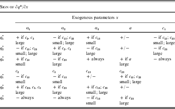
In general, the agent reacts to changes in incentive payments as shown in Table 1. The reaction of effort levels to the (indirect) incentives for the respective other activities depends on the substitutive or complementary nature of these activities. It is positive for the incentives for retirement and work out, as one of these two activities alleviates the effort costs for the other. The reaction to all other indirect incentives is negative, because the respective activities are substitutes to each other, either direct (work and work out) or indirect (work and retirement).
Comparative Statics of Effort Levels
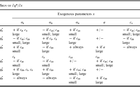
A special focus of this paper is on the variation of q 3 with respect to ability a. The effect cannot be qualified independently of a. For small a, the effect is negative, whereas for large a, I find a positive slope, such that the function q 3(a,⋅), holding everything else constant, is U-shaped. In general, see Table 1 for an overview of the sign of the derivatives of q* with respect to exogenous parameters. Interpretation of the partial effects of the exogenous parameters on ceteris paribus effort levels (for a given set of incentives) has to take into account that ‘small’ c 23 actually means |c 23| being large, hence the interaction of retirement and work out being strong. If, on the other hand, c 23 is large (close to zero), this is only compatible with negative incentives for retirement, hence with α2<0, which, however, is not ruled out; c 13 being small means that c 13 fulfills c 1c 3>c 132, which corresponds to the further condition in Table 1 of c 1 and c 3 being large.Footnote 9
Except for the derivatives of q 3 with respect to c 1, c 2, and c 3, none of the effects can be uniquely signed. The main determinants of ambiguous signs is the relative size of the cross derivatives of the cost function, hence of c 13 and c 23. This effect is due to their augmenting and reducing property in the cost function. If, for example, both cross derivatives are small, effort in activity work is decreasing in all c i and decreasing in c 23. Naïvely, effort levels should decline in direct effort costs. Here, also indirect effects play a role, such that q 2* reacts positively on all c i, because if effort costs are high, the best the agent can do is to delay retirement, in order to increase payments and to exploit the cost-reducing interaction with work out.
If the agent spends high effort on work, this increases the effort costs for work out. However, high costs for work out do not hurt so much, if the interaction of work out with retirement is strong. So once c 23 is already small (indicating a strong interaction), a further decrease away from zero increases the effort level for work.
First-best solution
The principal is risk neutral and the agent has exponential utility, hence maximization of joint surplus E(W)+U(t, q) is equivalent to the maximization of

where U CE is the certainty equivalent of U(t, q). The first-best solution is reached once all activities are deterministically translated into observed output, hence when all σi2 are zero. The incentives α* are then given by

The incentives are simply the weight the principal assigns to the respective activities. The optimal effort levels of the first-best solution are given once the general incentives αi in equation (17) are replaced by the weights in equation (20).
Second-best solution
Now, allowing for strictly positive elements in Σ, the second-best solution is again reached by maximization of the joint surplus

I refrain from the lump sum payment β, which I only use in order to fulfill the participation constraint U⩾Ū. The vector of marginal tax rates is given by

with α*=(α1* α2* α1*)′, I being the 3×3 identity matrix, c″ the 3×3 matrix of second derivatives of c(q), and w and Σ as defined in equations (9) and (11), respectively. Solving (22) explicitly, I have

with

In any case, α1* has always a different sign than α3*. The sign of α2* depends on the relative strength of the exogenous parameters – especially on the weight w 2 and the absolute size of c 23. Comparison of all αi* from the first-best with the second-best solution does not yield a clear answer and depends on the relative size of respective parameters, so incentives for work, retirement, and work out may be larger or smaller and can even be negative in all cases.Footnote 10
Since each of the optimal effort levels q depend on all αi, and the transition from first best to second best does not allow to sign all αi uniquely, the change of the optimal effort levels is also ambiguous. For the case of either work or work out being unobservable (hence, for σ12→∞ or σ32→∞ ), see Appendix A.
Comparative statics
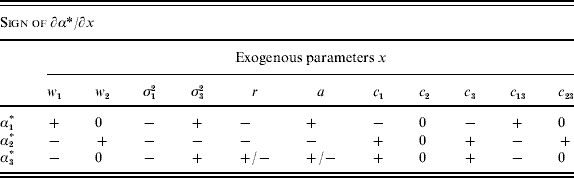
See Table 2 for a summary of comparative statics with respect to the exogenous parameters, computed under the already known assumption of c 13 being small.
Comparative Statics of Incentives
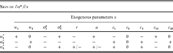
With the exception of the derivatives of α3* with respect to risk aversion r and ability a, all other derivatives of αi (i={1,2,3}) are uniquely signed. The weights have the predictable influence on incentives, namely that the higher the weight on a specific activity, the higher is the direct incentive. If another activity interferes, incentives for this alternative activity may decrease. Variance or risk in the observation of work reduces incentives for all activities in order to reduce the agent's exposure to that risk. Higher σ32 leads to a lower reward for delayed retirement and a higher reward for work, because the principal wants the agent to shift effort from one to the other.
The higher the effort costs for work, the lower are the respective incentives, because the principal urges the agent to shift attention from work to delayed retirement. This ceteris paribus result is already described in general by Holmstrom and Milgrom (Reference Holmstrom and Milgrom1991). Yet, the effort costs associated with delayed retirement have no influence on incentives, as this effort is perfectly observable and therefore enforceable. Even though the direct benefits of work out do not accrue to the principal, incentives change with the increased effort costs associated with it; the fraction of output from work that is distributed to the agent can be lower, while the reward for delayed retirement has to increase.
If the interaction between work and work out is strong, the principal is willing to pay more for work, while the payments for work out are even more discouraging. Yet, the interaction of retirement and work out does not change incentives for the latter, as retirement is perfectly observable and does not need high-powered indirect incentives. For larger c 23 (meaning, for c 23 being closer to zero), incentives for delayed retirement increase – in this case, external incentives have to substitute low internal incentives arising from the cost-decreasing interaction.
Now, focus on the important relationship between incentives and ability a. Incentives for work increase in ability, such that more able agents are encouraged to work more (e.g., by lower taxation for work), but incentives for delayed retirement actually decrease in a, which corresponds to higher implicit taxation or a progressive pension system. Finally, the relationship between incentives for work out and ability is not monotone. For small a, incentives decrease in a, whereas for large a, incentives increase. The thresholdFootnote 11 is at

meaning that the relationship is U-shaped in the positive domain of a and as long as all σi2 are finite.Footnote 12 Since actual effort levels correspond monotonically to incentives, investments in longevity and ability exert a U-shaped relationship as well. This phenomenon can be summarized and explained as follows.
An agent with low ability is encouraged to work out and to delay retirement, but not to work. This least able agent is not encouraged to both q 1 and q 3 at the same time, because of the cost augmenting interaction of both. The principal is better off when he provides incentives for the activities which interact as complements. A very able agent is encouraged to work and to work out, but not to delay retirement, which is not necessary, because the most able agent will choose relatively late retirement anyhow according to the interaction with his high effort in work out. But due to his high ability, it is worthwhile to encourage him to work as well. Eventually, an agent with intermediate ability is not encouraged to work out and faces moderate incentives for the other activities; incentives for q 3 are necessary only as a means to encourage either q 1 or q 2 indirectly. Here, incentives both facilitate work and delay retirement, such that the aggregate indirect effect of work out on effort costs at least partially cancels out, such that incentives for work out are not effective in promoting the other activities.Footnote 13
The result that incentives for work out or investments in longevity, as well as associated effort levels, are not monotone, but U-shaped in the agent's ability, relates to empirical findings, e.g. by von Gaudecker and Scholz (Reference Von Gaudecker and Scholz2007), Kibele (Reference Kibele2008), and Hupfeld (Reference Hupfeld2008). The downward-sloping area of the function that maps life expectancy to income may not be an artifact of the respective data sets or the methodology, but expression of the underlying economic mechanism outlined in this essay.Footnote 14
Conclusion
In a moral-hazard model with multiple activities, I model an agent who spends effort on work, retirement, and work out. The effort costs of these activities interact, such that work out increases costs for work, but decreases costs associated with delayed retirement. Under certain assumptions on the parameters, the second-best optimal incentives for work out are U-shaped in the agent's ability, and so is the optimal effort level in this activity. High incentives for work out for the least able encourage the agent to exploit the cost-reducing properties of the cost function and come with high incentives for the complement, namely delayed retirement. The most able agent faces high-powered incentives for work out mainly due to their indirect effect on delayed retirement, which allows to reduce incentives for this activity. In order to simultaneously promote work for the most able, incentives for it are high as well.
Of course, this model only serves as a first step from which further research on the potentially non-monotone relation between ability and longevity could depart. One direction includes the extension of multiple agents, either homogeneous or heterogeneous in ability. Risk will play a minor role in such a setting, once a relative incentive scheme is feasible for the principal.Footnote 15 Another direction may refine the labor supply decision of the agent and explicitly incorporate income effects, which work against a monotonically increasing labor supply, either instantaneous or with respect to retirement.
Empirically, the responsiveness of individual health-related behavior to adjustments in the pension system is widely neglected so far. For example Salm (Reference Salm2007) finds for US Army veterans that the sheer introduction of a pension system (in 1907 and 1912, respectively) increases life expectancy. Yet, the pure income effect of increased social security wealth cannot be disentangled from an actual adjustment of behavior.
Appendix: Optimal incentives with unobservable work or work out
If either one of the perturbed activities work or work out cannot be observed at all, optimal incentives are given by

with Ψ1=ac 1+rσ32(c 1c 3−c 132), and

with Ψ3=ac 3+rσ12(c 1c 3−c 132). Obviously, incentives cannot be conditioned on unobservable effort levels, but, more importantly, if one of the effort becomes unobservable, incentives for the other activities change. Focus on the latter, σ32→∞, which is more plausible (it is easier to observe and therefore to tax instantaneous labor supply than potentially private activities that enhance longevity). Assuming that risk aversion is larger than one, and σi2 being not smaller than one, I have Ψ3<Ψ. However, the denominator of αi*|σ32→∞, i=1, 2 is also smaller in the case of unobservable work out, such that the change of α1* and α1* is not uniquely signed.
 .