1. Introduction
Consider waves in an unbounded fluid governed by the two-dimensional Helmholtz equation,  $\phi _{xx}+\phi _{yy}+k^{2}\phi = 0$ for
 $(x,y)\in \varOmega$, where
 $\phi =\phi (x,y)\in \mathbb {C}$ is a (reduced) potential function and
 $k\in\mathbb{R}_{+}$ is a wavenumber that acts as a proxy for a prescribed angular frequency of motion. Let the fluid domain contain
 $N$ identical, equally spaced circular cylinders,
 $C_{1},\ldots,C_{N}$, of radius
 $a<0.5$, which are aligned along the
 $x$-axis with (dimensionless) unit centre-to-centre spacing, so that
 $\varOmega =\{(x,y): (x-n)^2+y^{2}>a^{2}, n=1,\ldots,N\}$. No-normal-flow conditions are applied on the cylinder boundaries,
 $\partial {}C_{n}=\{(x,y) : x=n+a\cos \theta _{n}, y=a\sin \theta _{n},\ \theta _{n}\in (-{\rm \pi},{\rm \pi} ]\}$ for
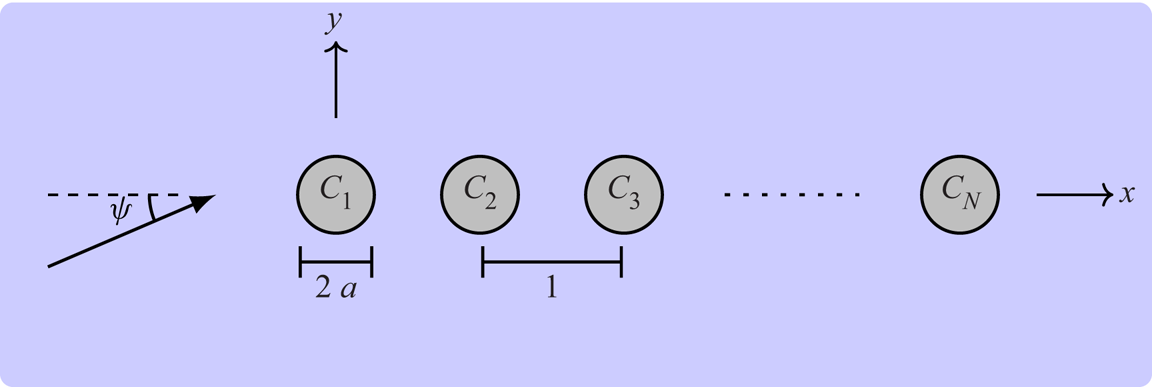
 $n=1,\ldots,N$, so that the cylinder may model sound-hard scatterers in an acoustic fluid or bottom-mounted surface-piercing columns in water (Martin Reference Martin2006). Motions are excited by a background (ambient) plane wave, propagating at an angle
 $\psi$ to the
 $x$-axis (figure 1).
Plan view of background wave and line array of  $N$ identical cylinders.

It would be reasonable to assume the wave field away from the array ends can be approximated by the corresponding infinite array ( $n\in \mathbb {N}$). But this is typically not true due to excitation of Rayleigh–Bloch waves, which propagate along the array with wavenumber
 $\beta (k)>k$, and decay exponentially away from it (Porter & Evans Reference Porter and Evans1999). They are unforced solutions of the infinite-array problem that exist for all
 $k\leq {}k_{{c}}<{\rm \pi}$, where
 $k_{{c}}(a)$ is known as the cutoff frequency. Plane waves cannot excite Rayleigh–Bloch waves along an infinite array as
 $\beta (k)>k$, but they can excite Rayleigh–Bloch waves along a semi-infinite array that propagate away from the end (Linton, Porter & Thompson Reference Linton, Porter and Thompson2007; Peter & Meylan Reference Peter and Meylan2007), or in both directions along a finite array (Thompson, Linton & Porter Reference Thompson, Linton and Porter2008).
Rayleigh–Bloch waves are a class of Bloch wave, familiar in the analysis of doubly periodic structures such as photonic/phononic crystals. Rayleigh–Bloch waves are the localised solutions obtained in the limit that the unit cell for a doubly periodic structure tends to infinity in one dimension (McIver Reference McIver2000), and, thus, they are also a class of trapped mode (Porter & Evans Reference Porter and Evans1999). In the limit, a continuous spectrum appears, and Rayleigh–Bloch waves (the discrete spectrum) are closely connected with embedded trapped modes (Linton & McIver Reference Linton and McIver2007), otherwise known as bound states in the continuum (Hsu et al. Reference Hsu, Zhen, Stone, Joannopoulos and Soljačić2016).
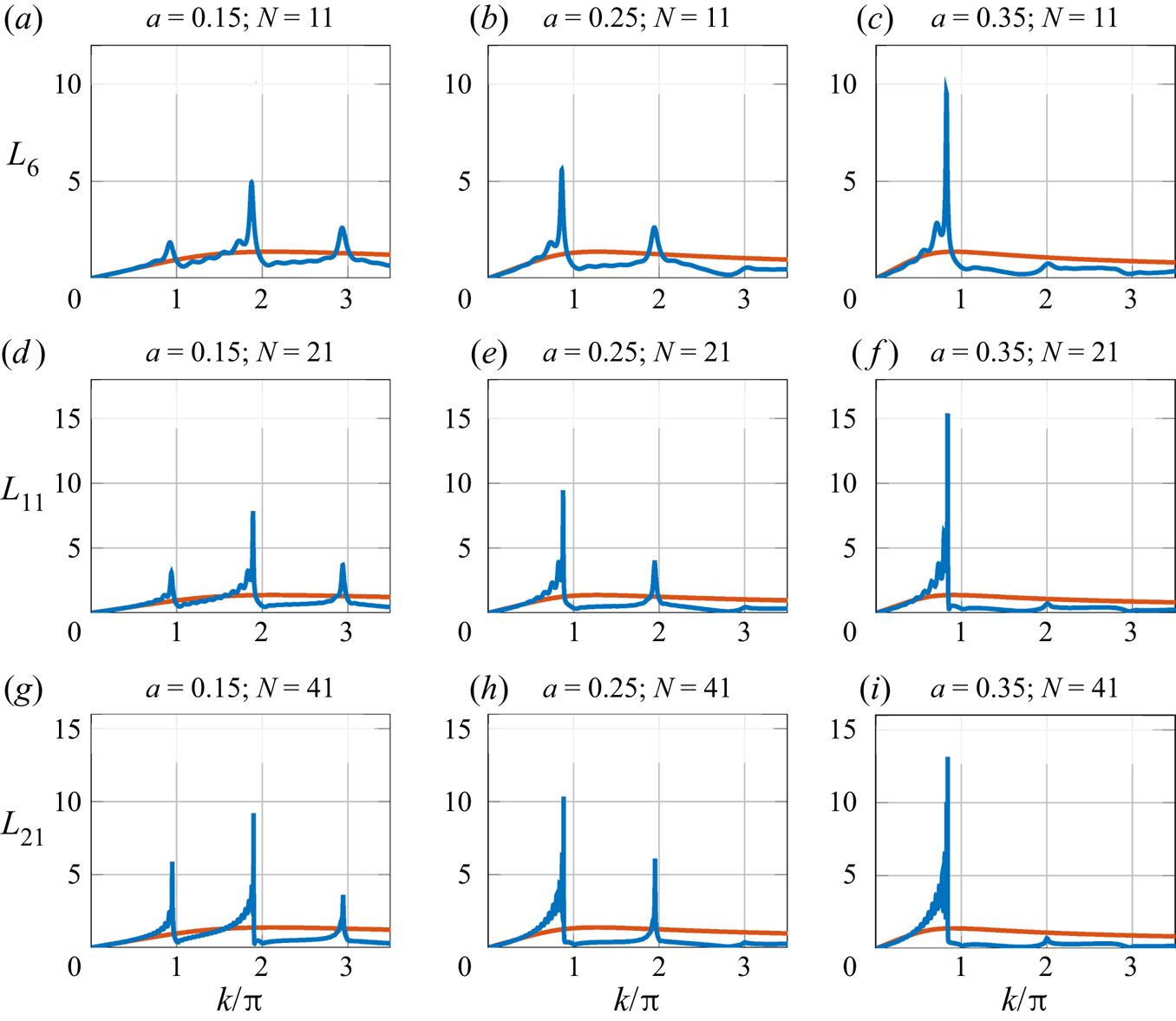
Maniar & Newman (Reference Maniar and Newman1997)'s discovery of resonant (water-wave) loads on finite arrays motivated a series of studies into Rayleigh–Bloch waves. Figure 2 shows the normalised  $x$-component of the dynamic load on the middle cylinder,
 $L_{\lceil {}N/2\rceil }$, where
 \begin{equation} {L_{n} = \frac{1}{\rm \pi}\left\vert\int_{-{\rm \pi}}^{\rm \pi} \left\{\cos(\theta_{n})\phi(n+a\cos\theta_{n},a\sin\theta_{n})\right\}\,\mathrm{d}\theta_{n}\right\vert\quad (n=1,\ldots,N),} \end{equation}
as a function of frequency, for  $\psi =0$ and different values of cylinder radius and array length. Loads on corresponding isolated cylinders are shown for reference. Primary resonances occur below
 $k={\rm \pi}$ in all cases, secondary resonances below
 $k=2{\rm \pi}$ for the small and intermediate cylinder radius values, and tertiary resonances below
 $k=3{\rm \pi}$ for the small-radius arrays. Each resonance is preceded by a series of sub-resonances that increase in number and become sharper as the length of the array increases. In other frequency intervals, the loads display relatively small oscillations (studied by Zeng et al. Reference Zeng, Yu, Shi and Wang2019).
Normalised load on middle cylinder in array vs frequency (blue curves) and single cylinder reference (red), for  $\psi =0$.

Maniar & Newman (Reference Maniar and Newman1997) connected primary resonances to trapped modes in channels containing a single cylinder along the centreline and Neumann conditions on the side walls, which exist at  $k=k_{{Neu}}(a)$ just above the resonant frequencies for all radius values. Similarly, they connected secondary resonances to channel modes with Dirichlet conditions applied on the channel walls, which exist at
 $k=k_{{Dir}}(a)$ up to
 $a\approx {}0.3394$ (Evans & Porter Reference Evans and Porter1998), explaining the absence of secondary resonances for the large-radius arrays in figure 2. Utsunomiya & Eatock Taylor (Reference Utsunomiya and Eatock Taylor1999) showed primary resonances are more accurately approximated by one of the trapped modes in a channel containing the full
 $N$-cylinder array and with Dirichlet wall conditions (for which there are
 ${\leq }N$ trapped modes), and that other trapped modes approximate sub-resonances.
Rayleigh–Bloch waves are equivalent to Neumann modes in the standing-wave limit  $\beta \to {\rm \pi}$ as
 $k\to {}k_{{Neu}}\equiv {}k_{{c}}$ (Porter & Evans Reference Porter and Evans1999). Evans & Porter (Reference Evans and Porter1999) gave evidence Rayleigh–Bloch waves are responsible for primary resonances, and derived the approximation
 $\beta \approx {}(N-1){\rm \pi} /N$ at the primary resonance, based on the Rayleigh–Bloch wave being a modulated Neumann mode. The studies connecting Rayleigh–Bloch waves with primary resonances culminated in Thompson et al. (Reference Thompson, Linton and Porter2008) showing resonant responses are due to constructive interference between Rayleigh–Bloch waves after reflections by the array ends.
Rayleigh–Bloch waves have only been found for certain parameter combinations above the cutoff (Porter & Evans Reference Porter and Evans2005), where they are embedded in the continuous spectrum, i.e. at frequencies that permit energy radiation away from the (infinite) array. Thus, secondary resonances and above for finite arrays have not been connected with Rayleigh–Bloch waves. Tertiary and quaternary resonances have been connected to higher-order Neumann and Dirichlet modes, respectively (Maniar & Newman Reference Maniar and Newman1997; Evans & Porter Reference Evans and Porter1998). However, similarly to Rayleigh–Bloch waves above the cutoff, higher-order Neumann and Dirichlet modes are embedded in the continuous spectrum and exist only for particular parameter combinations, whereas higher-order resonances exist over parameter intervals.
In this paper, we show extensions of Rayleigh–Bloch waves exist for frequency intervals above the cutoff, in which their wavenumbers become complex valued and a second type of Rayleigh–Bloch wave often exists. We propose a method that combines a transfer operator (cf. Bennetts Reference Bennetts2011; Montiel, Squire & Bennetts Reference Montiel, Squire and Bennetts2015) for a channel with generalized (quasi-periodic) boundary conditions on the side walls, and an artificial damping in the cylinder boundary conditions to separate the discrete and continuous spectra, and, thus, identify the extended Rayleigh–Bloch waves. The extended Rayleigh–Bloch waves are linked to the higher-order, finite-array resonances shown in figure 2, and, in most cases (but not all), existence of extended Rayleigh–Bloch waves for  $k$ just below multiples of
 ${\rm \pi}$ generates resonance.
2. Transfer operator for a generalized channel
Let  $\varOmega _{\textit {ch}}=\{(x,y):-0.5< x<0.5,\ y\in \mathbb {R}, (x,y)\notin {}C\}$ be a unit-width channel that contains a single cylinder
 $C=\{(x,y):x^{2}+y^{2}\leq {}a^{2}\}$ at its centre. A family of potential functions,
 $\{\phi =\phi (x,y\,|\,\mu ):\mu \in \varUpsilon \}$, are sought that satisfy the Helmholtz equation,
 \begin{equation} \phi_{xx}+\phi_{yy}+k^{2}\phi = 0 \quad\text{for}\ (x,y)\in\varOmega_{{ch}}, \end{equation}
and the cylinder boundary condition
 \begin{equation} \phi_{r}+\mathrm{i}\varepsilon \phi = 0 \quad\text{for}\ (x,y)\in\partial{}C = \{(x,y):x^{2}+y^{2}=a^{2}\}, \end{equation}
where  $\varepsilon \in \mathbb {R}$ is a (small) artificial damping parameter introduced to facilitate calculation of Rayleigh–Bloch waves above the cutoff in § 3. The solutions are parameterised by
 $\mu \in \mathbb {C}$, which defines the generalized channel boundary conditions (quasi-periodicities)
 \begin{equation} \phi(0.5,y)=\mu\phi({-}0.5,y) \quad\text{and}\quad \phi_{x}(0.5,y)=\mu\phi_{x}({-}0.5,y), \end{equation}
so that the solutions can be interpreted as infinite-array solutions. The set  $\varUpsilon$ defines the spectrum of possible solutions, which are defined up to constant multipliers (as radiation conditions are not prescribed). The spectrum is partitioned as
 $\varUpsilon =\varUpsilon _{{cts}}\cup \varUpsilon _{{dis}}$, where
 $\varUpsilon _{{cts}}$ is the continuous spectrum that defines forced solutions, i.e. involving a background wave, and
 $\varUpsilon _{{dis}}$ is the discrete spectrum that defines unforced solutions, i.e. Rayleigh–Bloch waves.
A potential satisfying (2.1) can be expressed as a superposition of the plane waves
 \begin{equation} \varphi_{{\pm}}(x,y{\,|\,}\chi)=\exp\{\mathrm{i} k\left((x\mp{}0.5)\cos\chi+y\sin\chi\right)\} \end{equation}
over directions  $\chi \in \varGamma =\{\gamma \in \mathbb {R}:-{\rm \pi} /2<\gamma <{\rm \pi} /2\}\cup \{\pm ({\rm \pi} /2-\mathrm {i}\gamma ):\gamma \in \mathbb {R}_{+}\}$, such that
 \begin{equation} \phi(x,y)=\int_{\varGamma}{A}_{{\pm}}(\chi)\varphi_{{\pm}}(x,y{\,|\,}\chi)\,\mathrm{d}{}\chi+ \int_{\varGamma}{B}_{{\pm}}(\chi)\varphi_{{\pm}}(x,y{\,|\,}\chi+{\rm \pi})\,\mathrm{d}{}\chi,\quad(x,y)\in\varOmega_{{\pm}}, \end{equation}
where  $\varOmega _{\pm }=\{(x,y):(x,y)\in \varOmega _{{ch}}, \pm {}x>0\}$. The amplitude functions
 ${A}_{\pm }$ (for components propagating or decaying rightwards, i.e. in the positive
 $x$-direction) and
 ${B}_{\pm }$ (leftwards) are related via
 ${B}_{-}=\mathcal {R}\{{A}_{-}\}+ \mathcal {T}\{{B}_{+}\}$ and
 ${A}_{+}=\mathcal {T}\{{A}_{-}\}+ \mathcal {R}\{{B}_{+}\}$. The reflection and transmission operators,
 $\mathcal {R}$ and
 $\mathcal {T}$, are defined for some arbitrary amplitude function
 $\bullet$ as, respectively,
 \begin{equation} \mathcal{R}\{{\bullet}\}=\frac{1}{\rm \pi}\int_{\varGamma}R(\chi{,}\psi)\bullet(\psi)\,\mathrm{d}\psi\quad\text{and}\quad \mathcal{T}\{{\bullet}\}=\frac{1}{\rm \pi}\int_{\varGamma}T(\chi{,}\psi)\bullet(\psi)\,\mathrm{d}\psi, \end{equation}
where
 \begin{equation} R(\chi{,}\psi)= \exp\left({\frac{\mathrm{i} k(\cos\chi+\cos\psi)}{2}}\right) \sum_{m={-}\infty}^{\infty}Z_{m}\exp({\mathrm{i} m(\chi-\psi-{\rm \pi})}), \end{equation}
and
 \begin{equation} T(\chi{,}\psi)=\exp\left({\frac{\mathrm{i} k(\cos\chi+\cos\psi)}{2}}\right) \left\{\delta(\chi-\psi){\rm \pi} +\sum_{m={-}\infty}^{\infty}Z_{m}\exp({\mathrm{i} m(\chi-\psi)})\right\}{.} \end{equation}
The cylinder boundary condition (2.2) is satisfied by the coefficients
 \begin{equation} Z_{m}={-}\frac{k\,\mathrm{J}'_{m}(k{a}){+\mathrm{i}\varepsilon\,\mathrm{J}_{m}(ka)}}{{k}\,\mathrm{H}'_{m}(k{a}) {+\mathrm{i}\varepsilon\,\mathrm{H}_{m}(ka)}}\quad\text{for}\ m\in\mathbb{Z}, \end{equation}
with  $\mathrm {J}_{m}$ and
 $\mathrm {H}_{m}$ order
 $m$ Bessel and Hankel functions of the first kind.
The transfer operator  $\mathcal {P}$ for the channel is such that (Bennetts, Peter & Montiel Reference Bennetts, Peter and Montiel2017)
 \begin{equation}
\left(\begin{array}{@{}c@{}}
{A}_{+}\\ {B}_{+} \end{array}\right)=\mathcal{P}
\left(\begin{array}{c} {A}_{-}\\ {B}_{-}
\end{array}\right)\quad\text{and}\quad
\mathcal{P}=\left(\begin{array}{c c}
\mathcal{T}-\mathcal{R}\mathcal{T}^{{-}1}\mathcal{R} &
\mathcal{R}\mathcal{T}^{{-}1}\\
\mathcal{T}^{{-}1}\mathcal{R} & \mathcal{T}^{{-}1}
\end{array}\right). \end{equation}
Therefore, the eigenfunctions of the transfer operator define the amplitude functions of quasi-periodic solutions (2.5), say  $A\equiv {}A_{-}=A_{+}/\mu$ and
 $B\equiv {}B_{-}=B_{+}/\mu$, and the eigenvalues
 $\mu \in \mathrm {eig}\{\mathcal {P}\}$ are the quasi-periodicities. The contour
 $\varGamma$ is truncated along its complex branches and discretised for computations (Montiel et al. Reference Montiel, Squire and Bennetts2015), so that the transfer operator becomes a transfer matrix and so on. If needed, transfer operators can be combined recursively (using the method of Bennetts & Squire Reference Bennetts and Squire2009) to obtain the solution for finite arrays, and give results indistinguishable to figure 2, which were calculated using Graf's addition theorem (as is standard; e.g. Peter & Meylan Reference Peter and Meylan2004; Linton & Thompson Reference Linton and Thompson2007).
3. Rayleigh–Bloch waves above the cutoff
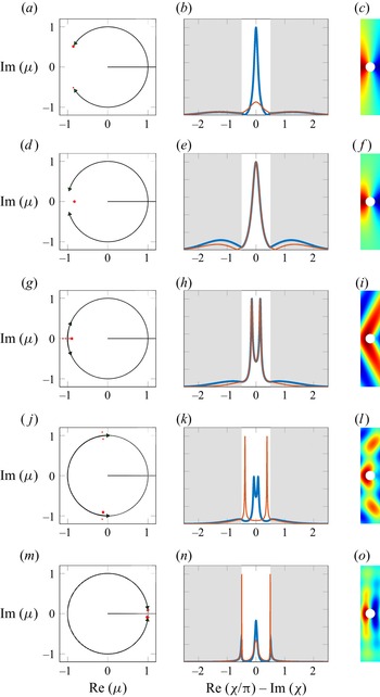
Figure 3 shows spectra of  $\mathcal {P}$ for radius
 $a=0.25$,
 $\varepsilon =0$, and frequencies from
 $k=0.8{\rm \pi}$ (a–c) to
 $1.95{\rm \pi}$ (m–o). Figure 3(a,d,g,j,m) shows the eigenvalues of
 $\mathcal {P}$ in the complex plane, divided into approximations of the continuous spectra (closely spaced black bullets) and the discrete spectra (red bullets). Figure 3(b,e,h,k,n) shows moduli of the eigenfunctions corresponding to the discrete-spectra eigenvalues indicated in (a,d,g,j,m) (large red bullets), with background shading used to distinguish the propagating and decaying components. Figure 3(c, f,i,l,o) shows the real parts of the modes corresponding to the indicated eigenvalues, i.e. Rayleigh–Bloch waves.
(a,d,g,j,m) Continuous spectrum (small black bullets) and discrete spectrum (red bullets). (b,e,h,k,n) Moduli of eigenfunctions ( ${A}(\chi )$ thick blue and
 ${B}(\chi )$ thin red) corresponding to highlighted eigenvalue (large red bullets in a,d,g,j,m), where the propagating components (
 $\chi \in \mathbb {R}$; white background) and decaying (
 $\chi \in \mathbb {C}$; grey) are indicated. (c, f,i,l,o) Real parts of corresponding modes for
 $-0.5< x<0.5$ and
 $-5< y<5$. Results are shown for (a–c)
 $k/{\rm \pi} = 0.8$, (d–f) 0.9, (g–i) 1.119, (j–l) 1.5, and (m–o) 1.95.

Eigenvalues in the continuous spectrum are  $\mu \in \varUpsilon _{\textit{c{ts}}}=\{\exp (\pm \mathrm {i} k\cos \chi ):\chi \in \varGamma \}$, and have multiplicity at least two due to symmetry of directional space, i.e. a prescribed quasi-periodicity can be created by an odd or an even background wave. Eigenvalues around the unit circle are solutions for propagating background waves (
 $\chi \in \mathbb {R}$), and those on the positive real axis for background waves growing/decaying in the
 $x$-direction (
 $\chi \in \mathbb {C}$). For frequencies such that
 $k<{\rm \pi}$, the propagating part of the continuous spectrum occupies only an arc of the unit circle with tips
 $\mu =\exp \{\pm \mathrm {i} k\}$ (i.e.
 $\psi =0$), so the arc occupies a greater proportion of the unit circle as frequency increases (figure 3a,d). The tips meet at
 $\mu =-1$ when
 $k={\rm \pi}$, i.e. the channel width is half the background wavelength, at which point the continuous spectrum occupies all of the unit circle. For
 $k>{\rm \pi}$, the continuous spectrum begins to overlap itself (figure 3g), which corresponds to additional scattering angles appearing, i.e. propagating waves in the far field at angles other than
 $\psi$ (see e.g. Peter, Meylan & Linton Reference Peter, Meylan and Linton2006; Linton & Thompson Reference Linton and Thompson2007).
For frequencies below the cutoff,  $k_{{c}}\approx {}0.89{\rm \pi}$, the discrete spectrum contains a reciprocal pair of eigenvalues,
 $\varUpsilon _{{dis}}=\{\mu =\exp (\pm \mathrm {i}\beta )\}$, where
 $\beta\in\mathbb{R}_{+}$ is the Rayleigh–Bloch wavenumber. The eigenvalues lie on the unit circle just ahead of the continuous-spectrum tips (figure 3a), as
 $\beta >k$, i.e. the Rayleigh–Bloch wavelength is shorter than that of the background medium. The eigenvalues in the upper (
 $\exp \{\mathrm {i}\beta \}$) and lower (
 $\exp \{-\mathrm {i}\beta \}$) halves of the complex plane define Rayleigh–Bloch waves propagating rightwards and leftwards, respectively. The eigenfunction for
 $\mu =\exp \{\mathrm {i}\beta \}$ has a rightward-propagating component (
 ${A}(\chi )$ for
 $-0.5<\chi /{\rm \pi} <0.5$) that outweighs the leftward-propagating component (
 ${B}(\chi )$), which is consistent with the Rayleigh–Bloch wave propagating rightwards (figure 3b). The eigenfunction for
 $\mu =\exp \{-\mathrm {i}\beta \}$ is deduced from reciprocity, i.e.
 $A$ and
 $B$ swapped, and, hence, leftward propagation of the Rayleigh–Bloch wave is inferred. The Rayleigh–Bloch modes are localised to the array as anticipated (figure 3c for
 $\mu =\exp \{\mathrm {i}\beta \}$). As frequency increases, the eigenvalues in the discrete spectrum move around the unit circle ahead of the tips of the continuous spectrum and the amplitude functions become closer to one another, indicating that the Rayleigh–Bloch group velocity is slowing. At the cutoff frequency,
 $k=k_{{c}}\equiv {}k_{{Neu}}$, the eigenvalues meet at
 $\mu =-1$ (
 $\beta ={\rm \pi}$), at which point the Rayleigh–Bloch waves cease propagating (
 $A=B$) and become the Neumann mode.
For frequencies just above the cutoff, the eigenvalues move onto the negative real axis (figure 3d), i.e.  $\beta ={\rm \pi} +\mathrm {i}{\gamma }$ where
 ${\gamma }\in \mathbb {R}_{+}$. By reciprocity, one eigenvalue lies inside the unit circle and the other outside (the latter is beyond axes limits). Thus, the extensions of the Rayleigh–Bloch waves above the cutoff decay along the array, which can be inferred from
 $A$ and
 $B$ only differing along the complex branches of
 $\varGamma$ (figure 3e, grey regions). The modes remain localised to the array (figure 3f).
The eigenvalues move farther away from the unit circle along the negative real axis (increasing  $\gamma$) until
 $k\approx {}1.01{\rm \pi}$, at which point they move back towards the unit circle (decreasing
 $\gamma$; figure 3g). The smooth peaks in the eigenfunctions around
 $\chi =0$ split into pairs of sharper peaks (figure 3h), which generate approximately plane decaying wave components in the modes, causing them to stretch farther away from the array (figure 3i). At
 $k\equiv {}k_{\to }\approx {}1.1{\rm \pi}$, an additional reciprocal pair of eigenvalues join the discrete spectrum, emanating from the continuous spectrum at
 $\mu =-1$ (visible in figure 3g), so that there is a second Rayleigh–Bloch wavenumber
 $\beta ={\rm \pi} +\mathrm {i}\delta$ (
 $\delta <\gamma$).
The additional eigenvalues move away from the unit circle along the negative real axis (increasing  $\delta$) until they collide with the original eigenvalues at
 $ k\equiv {}k_{{\nearrow\hspace{-10.5pt}\searrow}} \approx {} 1.12{\rm \pi}$ (
 $\delta =\gamma$; not shown). One eigenvalue in each collision moves into the upper-half complex plane and the other into the lower-half, so that the Rayleigh–Bloch wavenumber pair is of the form
 $\beta \equiv \beta _{\pm }={\rm \pi} \pm \alpha +\mathrm {i}\gamma$ with
 $\alpha,\gamma \in \mathbb {R}_{+}$. The eigenvalue pairs in the upper and lower halves of the complex plane chase their respective continuous-spectrum tips around the unit circle (figure 3j). For the highlighted eigenvalue,
 $\mu =\exp \{\mathrm {i}\beta _{+}\}$, the peaks in
 $A$ tend towards
 $\chi =0$ and become smoother, whereas the peaks in
 $B$ tend towards
 $\chi =\pm {}{\rm \pi} /2$ and become sharper (figure 3k). The mode stretches increasingly far away from the array and complicated interference patterns develop around the array (figure 3l). Just below the Dirichlet-mode frequency,
 $k=k_{{Dir}}(0.25)\approx {}1.9555{\rm \pi}$, the eigenvalues overtake the tips of the continuous spectrum and tend towards the continuous spectrum on the unit circle (figure 3m). Both rightward and leftward components of the eigenfunction display smooth peaks around
 $\chi =0$, similar to below the cutoff, and sharp peaks close to
 $\chi =\pm {}{\rm \pi} /2$ (figure 3n). Cancellation of the sharp peaks causes the modes to regain array localisation (figure 3o).
Identifying the discrete spectrum becomes increasingly difficult as it tends towards the continuous spectrum. Introducing damping ( $\varepsilon \neq {}0$) moves half of the discrete spectrum away from the continuous spectrum and half towards it, where the sign of
 $\varepsilon$ determines which eigenvalue pair moves away from the unit circle (and which pair moves towards it). In contrast, the continuous spectrum remains in
 $\varUpsilon _{{c{ts}}}$ as the background waves dictate the quasi-periodicities of the solutions. Suitable choices of
 $\varepsilon$ make it possible to identify the discrete spectrum as the frequency passes through the Dirichlet mode. At each frequency, homotopy is used to obtain the discrete spectrum for the original (undamped) problem, by decreasing
 $\vert \varepsilon \vert$ to zero in small steps and tracking the eigenvalue–eigenfunction pairs.
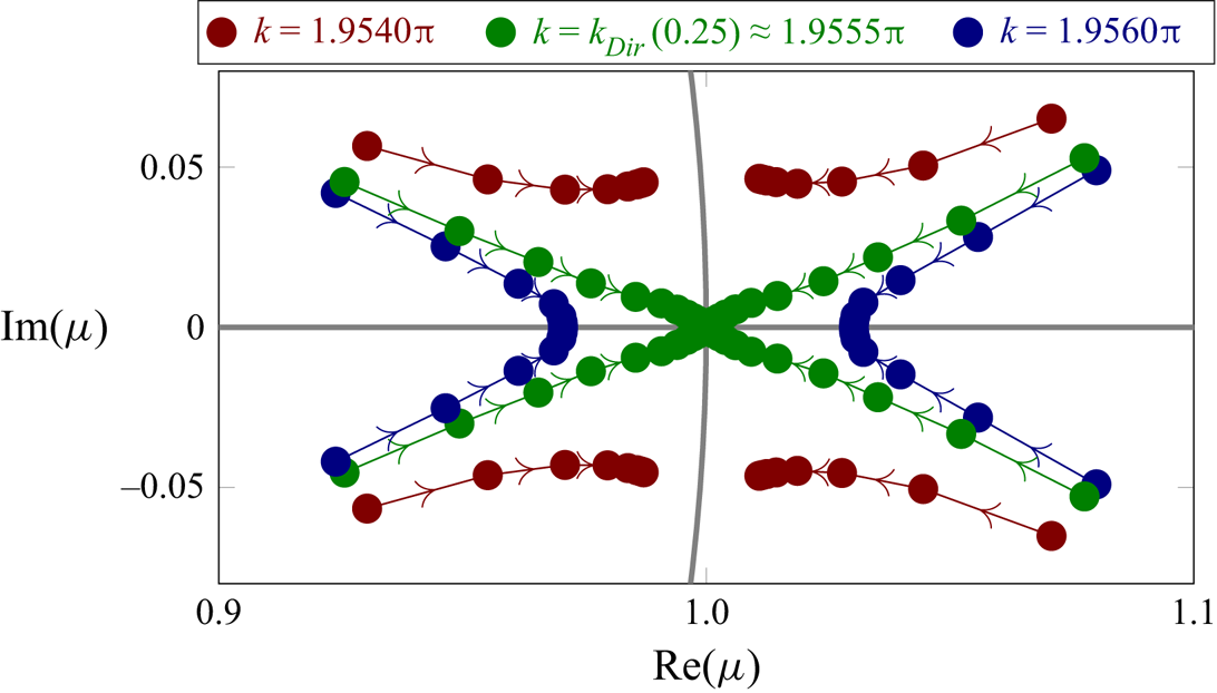
Figure 4 illustrates the homotopy method and shows the discrete spectrum below, at and above the Dirichlet mode frequency. Below the Dirichlet mode frequency, the discrete spectrum is of the form  $\varUpsilon _{{dis}}=\{\mu =\exp (\pm \mathrm {i}\beta _{\pm })\}$ and close to the unit circle (
 ${\gamma }\ll {}1$). At
 $k=k_{{Dir}}\approx {}1.9555{\rm \pi}$, the four eigenvalues coalesce at
 $\mu =1$, i.e.
 $\beta =2{\rm \pi}$ (or
 $=0$), at which point the extended Rayleigh–Bloch waves become the Dirichlet mode. Above the Dirichlet mode, the discrete spectrum contains a reciprocal pair of eigenvalues that lie on the positive branch of the real axis, embedded in the continuous spectrum, so that there is a single Rayleigh–Bloch wavenumber,
 $\beta =2{\rm \pi} +\mathrm {i}\gamma$ for
 $\gamma \in \mathbb {R}_{+}$. The discrete spectrum vanishes into the continuous spectrum for
 $k\approx {}2{\rm \pi}$, i.e. all eigenvalues
 $\mu \in \varUpsilon _{{c{ts}}}$ irrespective of the
 $\varepsilon$-value.
Discrete spectrum around Dirichlet mode frequency, for damping  $\vert \varepsilon \vert =0.2$ to 0.0001 with logarithmically scaled steps, where arrows indicate decreasing
 $\vert {}\varepsilon \vert$.

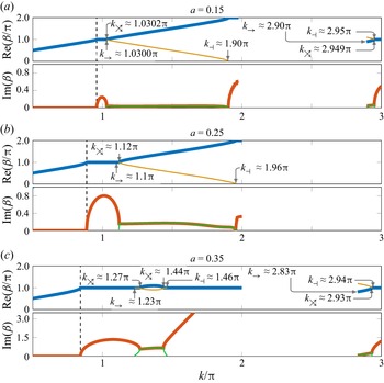
Figure 5 shows the Rayleigh–Bloch dispersion curves for the small, intermediate and large radii up to  $k=3{\rm \pi}$. The dispersion curves for the intermediate radius (
 $a=0.25$; figure 5b) follow the above analysis, with a single
 $\beta \in \mathbb {R}$ for
 $k\leq {}k_{{c}}\approx {}0.89{\rm \pi}$,
 $\beta ={\rm \pi} +\mathrm {i}{\gamma }$ for
 $k_{{c}}< k<1.12{\rm \pi}$ and joined by a second
 $\beta ={\rm \pi} +\mathrm {i}\delta$ (
 $\delta <\gamma$) for
 $1.1{\rm \pi} < k<1.12{\rm \pi}$, two complex-valued
 $\beta ={\rm \pi} \pm {\alpha +\mathrm {i}\gamma }$ for
 $1.12{\rm \pi} < k<1.96{\rm \pi}$, and a single
 $\beta =2{\rm \pi} +\mathrm {i}{\gamma }$ for
 $1.96{\rm \pi} < k<2{\rm \pi}$. There is only evidence of a continuous spectrum for
 $k>2{\rm \pi}$.
Rayleigh–Bloch-wave dispersion curves. Real parts (thick blue and thin yellow curves), imaginary parts (thick red and thin green) and cutoff frequencies (broken black).

The dispersion curves for the small radius ( $a=0.15$; figure 5a) are qualitatively similar to the intermediate radius for
 $k<2{\rm \pi}$, with the most notable difference being the shorter interval for which
 $\beta ={\rm \pi} +\mathrm {i}{\gamma }$ above the cutoff. In contrast to the intermediate radius, the discrete spectrum reappears at
 $k_{\rightarrow }\approx {}2.90{\rm \pi}$, with four eigenvalues emanating from the continuous spectrum on the unit circle just behind the tips of the continuous spectrum, defined by a pair of complex-valued Rayleigh–Bloch wavenumbers
 $\beta =\pm \alpha +\mathrm {i}\gamma$. The eigenvalues move slightly away from the unit circle (increasing
 $\gamma$) and follow the continuous-spectrum tips around the unit circle (
 ${\alpha }\to {}{\rm \pi}$) until
 $k_{{\nearrow\hspace{-10.5pt}\searrow}}\approx {}2.949{\rm \pi}$, when pairs of eigenvalues meet on the negative real axis (one pair inside and one outside) and then move in opposite directions along the real axis, so that
 $\beta ={\rm \pi} +\mathrm {i}\gamma$ and
 $\beta ={\rm \pi} +\mathrm {i}\delta$ (
 $\delta <\gamma$), where
 $\gamma$ increases with frequency and
 $\delta$ decreases. At
 $k_{\dashv }\approx {}2.95{\rm \pi}$, the eigenvalues
 $\mu =\exp \{\pm \mathrm {i}({\rm \pi} +\mathrm {i}\delta )\}$ vanish into the continuous spectrum at
 $\mu =-1$ (
 $\delta \to {}0$), so that the second Rayleigh–Bloch wavenumber no longer exists, leaving only a single wavenumber
 $\beta ={\rm \pi} +\mathrm {i}\gamma$ that defines a reciprocal eigenvalue pair in the discrete spectrum,
 $\mu =\exp \{\pm \mathrm {i}({\rm \pi} +\mathrm {i}\gamma )\}$, which tends towards the origin from below and negative infinity (increasing
 $\gamma$).
The dispersion curves for the large radius ( $a=0.35$; figure 5c) are qualitatively similar to those for the smaller radii for frequencies only up to where the pair of eigenvalues that emerge from the continuous spectrum above the cutoff collide with the existing eigenvalues at
 $k_{{\nearrow\hspace{-10.5pt}\searrow}}\approx {}1.27{\rm \pi}$ and move into the complex plane. Rather than following the tips of the continuous spectrum around the unit circle, the eigenvalues move back towards the negative real axis where they collide for a second time and then move in opposite directions along the negative real axis. The eigenvalues moving towards the unit circle vanish into the continuous spectrum at
 $k_{\dashv }\approx {}1.46{\rm \pi}$, whereas the remaining eigenvalue pair tends towards the origin/infinity. The discrete spectrum reappears at
 $k_{\rightarrow }\approx {}2.83{\rm \pi}$ and has similar qualitative behaviour to the discrete spectrum for
 $a=0.15$ below
 $k=3{\rm \pi}$.
4. Connection to resonances along finite arrays
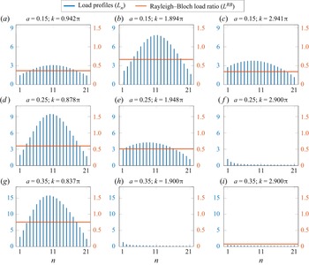
Figure 6 shows load profiles along  $21$-cylinder arrays for
 $a=0.15$, 0.25 and 0.35, at frequencies below
 $k={\rm \pi}$,
 $2{\rm \pi}$ and
 $3{\rm \pi}$. In cases where Rayleigh–Bloch waves exist, i.e. frequency intervals occupied by dispersion curves in figure 5, the ratio
 $L^{{RB}}=L^{{RB}}_{-}/L^{{RB}}_{+}$ is also shown, where
 $L^{{RB}}_{\pm }$ are the loads imposed by the leftwards (
 $-$) and rightwards (
 $+$) propagating/decaying Rayleigh–Bloch waves, which are calculated by decomposing the wave field into the transfer operator modes. Above the cutoff, where
 $\beta \in \mathbb {C}$, the ratios are scaled by
 $\exp \{2\,{\rm Im}(\beta )(n-1)\}$ to remove dependence on the index
 $n$. In cases where four (extended) Rayleigh–Bloch waves exist, the Rayleigh–Bloch waves that create the greatest loads are used to calculate
 $L^{{RB}}$.
Load profiles along 21-cylinder arrays for  $\psi =0$ (blue bars), and ratio of loads imposed by leftwards propagating/decaying Rayleigh–Bloch waves to rightwards propagating/decaying Rayleigh–Bloch waves (red lines).

The frequencies below the cutoffs (a,d,g) are at the primary resonance peaks (cf. figure 2d–f). In each case, the rightward-propagating Rayleigh–Bloch wave causes consistently greater loads than the leftward-propagating Rayleigh–Bloch wave, although the loads are of comparable magnitude as indicated by the  $L^{{RB}}$-values. Coherence between the rightward- and leftward-propagating Rayleigh–Bloch waves near the array centre (
 $\beta \approx {}(N-1){\rm \pi} /N$) creates the characteristic near-symmetric resonant-load profiles.
For the small- and intermediate-radius cylinders, the frequencies below  $k=2{\rm \pi}$ (figure 6b,e) are at the secondary resonance peaks. Four extended Rayleigh–Bloch waves exist (figure 5a,b), decaying rightwards (
 ${\beta =}{\rm \pi} \pm {\alpha }+\mathrm {i}{\gamma }$) or leftwards (
 ${\beta =}{\rm \pi} \pm {\alpha }-\mathrm {i}{\gamma }$) along the array, and the resonant frequencies coincide with coherence, such that
 ${\alpha }\approx {}(N-1){\rm \pi} /N$. The dominant Rayleigh–Bloch waves decaying rightwards and leftwards have
 ${\beta =}{\rm \pi} +{\alpha }\pm \mathrm {i}{\gamma }$. They generate loads of comparable magnitude, as indicated by the
 $L^{{RB}}$-values. For the small radius, the resonant-load profile is similar to those below the cutoff, but for the intermediate radius the profile is skewed towards the array front due to skewing of the coherence (not shown).
For the large radius (figure 6h), no resonance or extended Rayleigh–Bloch waves exist below  $k=2{\rm \pi}$ (figures 2 f and 5c). The chosen frequency is close to those for
 $a=0.15$ and 0.25, but the cylinder loads are small and the profile tends to decrease along the array, as diffraction dominates the response in the absence of Rayleigh–Bloch waves.
Only the small-radius array has a resonance below  $k=3{\rm \pi}$ (figure 2d), and the load profile at the resonance peak is shown (figure 6c). Four extended Rayleigh–Bloch waves exist (figure 5a), with wavenumbers
 ${\beta =}\pm (\pm {\alpha }+\mathrm {i}{\gamma })$, such that
 ${\alpha }\approx {}(N-1){\rm \pi} /N$. The dominant Rayleigh–Bloch waves have wavenumbers
 ${\beta =\alpha }\pm \mathrm {i}{\gamma }$, and, as with the previous resonances, they create loads of comparable magnitude. The load profile is skewed towards the array front, similar to the intermediate-radius resonance below
 $k=2{\rm \pi}$ (figure 6e).
Representative load profiles are shown for the intermediate- and large-radius arrays below  $k=3{\rm \pi}$. Both responses appear to be diffraction dominated, similar to the large-radius array below
 $k=2{\rm \pi}$. For the large radius, extended Rayleigh–Bloch waves exist below
 $3{\rm \pi}$ (figure 5c), and the frequency is chosen to satisfy the coherence condition. However, the ratio of loads imposed by the dominant Rayleigh–Bloch waves shows the leftward-decaying waves are an order of magnitude less than the rightward-decaying waves (
 $L^{{RB}}=0.079$), which precludes generation of resonance.
5. Summary and concluding remarks
Extensions of Rayleigh–Bloch waves above the cutoff have been calculated up to  $k=3{\rm \pi}$. An additional pair of Rayleigh–Bloch waves was found to emanate from the continuous spectrum and (typically) define a symmetric quartet of complex-valued wavenumbers. For small- to intermediate-radius cylinders, the extensions were shown to form continuous connections between the Neumann mode (at the cutoff frequency) and the Dirichlet mode, where the wavenumbers coalesce. Between the Neumann and Dirichlet modes, the Rayleigh–Bloch wave amplitude functions were found to develop spikes and, hence, lose array localisation. Above the Dirichlet mode, the Rayleigh–Bloch waves become embedded in the branch of the continuous spectrum associated with decaying background waves before they vanish. For a small-radius cylinder, they were found to reappear below
 $k=3{\rm \pi}$, and similar behaviour was found for a large-radius cylinder. Existence of extended Rayleigh–Bloch waves was related to resonances on finite arrays occurring for some radius values and not others, although an example was given to show that existence of Rayleigh–Bloch waves with wavenumbers satisfying a coherence condition does not guarantee resonance.
Rayleigh–Bloch waves are being used as a mechanism to control wave propagation in metamaterial-esque arrays, including ring resonators (Maling & Craster Reference Maling and Craster2016), graded resonator arrays (Bennetts, Peter & Craster Reference Bennetts, Peter and Craster2018), flat lensing meta-arrays (Chaplain & Craster Reference Chaplain and Craster2019) and superhydrophobic metasurfaces (Schnitzer, Brandão & Yariv Reference Schnitzer, Brandão and Yariv2019). The discovery of extended Rayleigh–Bloch waves creates the possibility of designing line arrays to control high-frequency waves. Moreover, the approach used in this study could be combined with the method of Bennetts, Peter & Craster (Reference Bennetts, Peter and Craster2019) to seek generalizations of Rayleigh–Bloch-type waves, and, hence, control wave propagation, at high frequencies for multiple-line arrays.
Funding
The work is supported by the Alexander von Humboldt Foundation. LGB is supported by the Australian Research Council (FT190100404).
Declaration of interests
The authors report no conflict of interest.