

I. INTRODUCTION
The self-consistent Hershey–Eshelby–Kröner–Kneer model is based on the original work of Eshelby (Reference Eshelby1957), which describes the interaction of an ellipsoidal inclusion in an isotropic polycrystalline matrix. Kröner (Reference Kröner1958) used the Eshelby inclusion as a basis for calculating the polycrystalline bulk (K) and shear modulus (G) from single crystal elastic constants of cubic symmetry. Both a quartic and a cubic polynomial of the shear modulus G with one positive real root were found. The quartic polynomial of G was found earlier by Hershey (Reference Hershey1954). Later, Kneer (Reference Kneer1963) generalized the procedure to crystallites of triclinic symmetry. Usually one refers to this as the self-consistent, Eshelby–Kröner, Kröner–Eshelby or Kröner model.
With the more recent publication of Behnken and Hauk (Reference Behnken and Hauk1986) the calculation of accurate X-ray Elastic Constants for triclinic crystal symmetry and all possible higher symmetry cases became possible. Until then only estimates based on the limiting models of Voigt (Reference Voigt1887) and Reuss (Reference Reuss1929) and the empirical Neerfeld–Hill average (Neerfeld, Reference Neerfeld1942; Hill, Reference Hill1952), were available. This is also called the Voigt–Reuss–Hill (VRH) average for calculating polycrystalline elastic properties in other fields (e.g. geophysics). The Hill average remained popular because of its ease of calculation and fairly accurate results for single phase polycrystals of moderate anisotropy.
As the Kröner model satisfies physical conditions of continuity and compatibility between the inclusion properties and the surrounding polycrystalline matrix, it has the fundamental ability to describe the elastic properties of multi-phase materials and the effects of inclusions or pores. For the approximate models, Voigt, Reuss, and Hill, one must resort to applying the rule of mixtures when dealing multiple phases, which can be successful for specific, limiting cases only (e.g. Kim et al., Reference Kim, Hong and Kim2001). In real polycrystalline materials, the presence of texture in the polycrystalline matrix can occur as well and the above-mentioned models can be extended to include texture information via the crystallite orientation distribution function (CODF). In this paper, we restrict the analysis to the case of a non-textured or isotropic polycrystalline matrix.
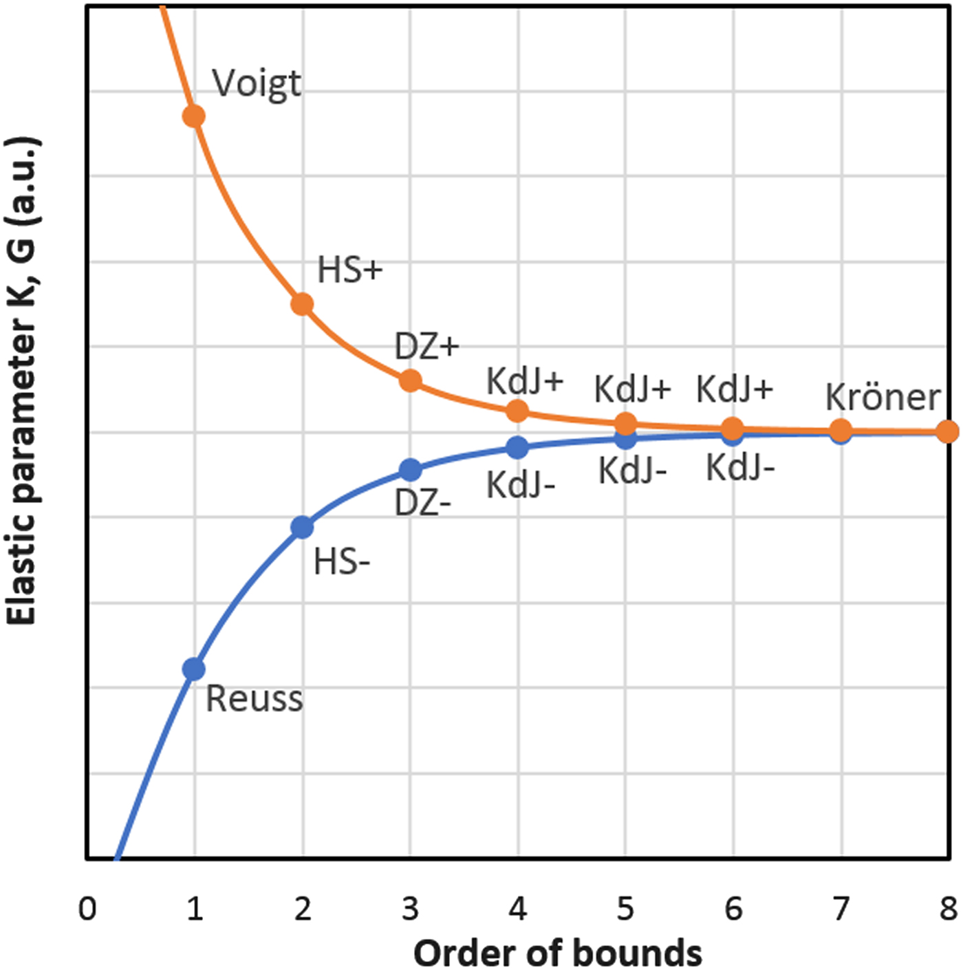
Recently Kube and de Jong (Reference Kube and de Jong2016) presented a new technique for the calculation of progressively narrowing bounds of isotropic polycrystalline elastic parameters, for example K and G, for polycrystals with any crystal symmetry. Earlier this was outlined by Kröner (Reference Kröner1978) and applied for polycrystalline aggregates of crystals of cubic symmetry by Gairola and Kröner (Reference Gairola and Kröner1981). The technique iterates over a series of either odd or even orders after applying respective initial seeds. The “narrowing bounds” model unifies all existing bounds/limits like Reuss (Reference Reuss1929), Voigt (Reference Voigt1887) as first order bounds, second order bounds: Hashin and Shtrikman (Reference Hashin and Shtrikman1962a, Reference Hashin and Shtrikman1962b), third order: Dederichs and Zeller (Reference Dederichs and Zeller1973). The fourth and higher orders are predicted by Kube and de Jong (Reference Kube and de Jong2016) and ultimately the nth bounds converge to a single solution that equals the self-consistent, Kröner model. Figure 1 provides an illustrative example. The numerical convergence is approximately an order of magnitude for each iteration step. Hence, only a few iterations are needed to find the Kröner limit.
Schematic illustration of the narrowing bounds model of Kube and de Jong (Reference Kube and de Jong2016). Their odd and even series of bounds are merged here into one graph for clarity. Hypothetical values. With (mathematical) initial seeds 0 or Infinity the first order Reuss and Voigt bounds are found respectively. Then with the next iteration the third order bounds of Dederichs and Zeller (DZ). And with more iterations the 5th and higher orders of Kube and de Jong (KdJ). With varying the crystal orientation the min() or max() values are used as (physical) initial seeds to find the second order Hashin–Shtrikman (HS) bounds. Then with more iterations the fourth and higher orders of Kube and de Jong (KdJ). Ultimately the nth order upper (“+”) and lower (“−”) bounds converge together to the Kröner solution.

II. THEORY
The calculations of the Kröner model can be approached in the following two steps. First, we find the polycrystalline elastic properties: the bulk modulus (or compressibility) K and the shear modulus G. Then secondly, we calculate the X-ray Elastic Constants (XEC) as required for residual stress measurements with X-rays, neutrons, or synchrotron radiation. This 2-step calculation scheme will also be applicable when calculating the response of the polycrystalline material to ultrasonic waves or other experimental techniques. The two steps are discussed next in reversed order for clarity.
A. X-ray elastic constants – final step
The X-ray elastic constants S 1 and ½S 2 are generally defined as (Stickfort, Reference Stickfort1966; Behnken and Hauk, Reference Behnken and Hauk1986):
 $$S_1 = \displaystyle{1 \over 2}{\bi a}_{ijkl}\gamma _i\gamma _j(\delta _{kl}-\gamma _k\gamma _l)\eqno \lpar1{\rm a}\rpar$$
 $$\displaystyle{1 \over 2}S_2 = \displaystyle{1 \over 2}{\bi a}_{ijkl}\gamma _i\gamma _j(3\gamma _k\gamma _l-\delta _{kl})\eqno \lpar1{\rm b}\rpar$$
where γ 1, γ 2, and γ 3 are crystallographic parameters depending on lattice constants (a, b, c, α, β, and γ) and Miller indices (hkl) (e.g. Gnäupel-Herold et al., Reference Gnäupel-Herold, Creuziger and Iadicola2012):
 $$\gamma _1 = d\left( {\displaystyle{h \over a}} \right)\eqno \lpar2{\rm a}\rpar$$
 $$\gamma _2 = d\left\{ {\displaystyle{{-\cos \,\gamma} \over {\sin \,\gamma}} \left( {\displaystyle{h \over a}} \right) + \displaystyle{1 \over {\sin \,\gamma}} \left( {\displaystyle{k \over b}} \right)} \right\}\eqno \lpar2{\rm b}\rpar$$
 $$\eqalign{\gamma _3 &= d\bigg( {\displaystyle{{abc} \over V}} \bigg)\bigg\{ {\displaystyle{{\cos \,\alpha \cos \,\gamma -\cos \,\beta} \over {\sin \,\gamma}} \bigg( {\displaystyle{h \over a}} \bigg) }\cr& \quad+ {\displaystyle{{\cos \,\beta \cos \,\gamma -\cos \,\alpha} \over {\sin \,\gamma}} \bigg( {\displaystyle{k \over b}} \bigg) + \sin \,\gamma \bigg( {\displaystyle{l \over c}} \bigg)} \bigg\}\eqno \lpar2{\rm c}\rpar$$
with d-spacing d (for triclinic symmetry, see e.g. Cullity, Reference Cullity1956) and volume V is defined as:
 $$V = abc\; (1-{\rm co}{\rm s}^2\,\alpha -{\rm co}{\rm s}^2\,\beta -{\rm co}{\rm s}^2\,\gamma + 2{\rm \;\ cos}\,\alpha \; {\rm cos}\,\beta \; {\rm cos}\,\gamma )^{1/2}\eqno \lpar2{\rm d}\rpar$$
The 4-rank tensor a is calculated according to either of the models Voigt, Reuss, Hill (see Appendix A) or Kröner. The general solution for the X-ray elastic constants with triclinic symmetry for the Kröner model has been first published by Behnken and Hauk (Reference Behnken and Hauk1986):
 $${\bi a}_{ijkl} = ({\bi S}_{ijkl} + {\bi t}_{ijkl})$$
where S is the isotropic polycrystalline compliance tensor. The tensor t describes the interaction of a spherical inclusion with the polycrystalline matrix. These tensors are independent of the crystallographic parameters and related only to the polycrystalline averages of the elastic parameters. A pair of two parameters will be sufficient, for example the bulk modulus K and the shear modulus G.
B. Polycrystalline elastic properties – initial step
The interaction tensor t is defined as (Behnken and Hauk, Reference Behnken and Hauk1986)
 $${\bi t}_{ijkl} = {\bi u}_{ij}^{.\, .\,mn} : {\bi S}_{mnkl}\; \eqno \lpar4{\rm a}\rpar$$
with (Einstein summation convention for indices m and n)
 $${\bi u}^{ijkl} = -({\bi v})^{-1,ijmn} : ({\bi c}_{mn}^{.\, .\,kl} -{\bi C}_{mn}^{.\, .\,kl} )\eqno \lpar4{\rm b}\rpar$$
where c (lowercase) is the single crystal stiffness tensor of the inclusion and C (uppercase) the isotropic stiffness tensor of the polycrystalline matrix.
The tensor v is (Einstein notation for indices m and n)
 $${\bi v}^{ijkl} = ({\bi c}^{ijkl}-{\bi C}^{ijkl}) + {\bi C}^{ijmn} : {\bi W}_{mn}^{.\, .\,kl} \eqno \lpar4{\rm c}\rpar$$
where W is the inverse of the isotropic Eshelby tensor.
The polycrystalline isotropic tensors C, S, and W depend only on the polycrystalline averages of the elastic parameters K and G (see Appendix B). The solution is found if one realizes that a polycrystalline aggregate (the matrix) is composed of many single crystallites (the inclusion) each with a possibly unique orientation. The polycrystalline average is found by averaging over all possible orientations of the inclusion. Hence, it must hold that
 $${\rm \langle} {\bi t}_{ijkl} = 0{\rm \rangle} \eqno \lpar5{\rm a}\rpar$$
or
 $${\rm \langle} {\bi u}_{ijkl} = 0{\rm \rangle} \eqno \lpar5{\rm b}\rpar$$
If all orientations occur with the same probability (i.e. random orientation, no texture), we can optimize guesses for polycrystalline parameters K and G such that Eqs (5ab) are satisfied.
Unfortunately, how the averaging of the tensors in Eqs (5ab) is to be done is not explained in Behnken and Hauk (Reference Behnken and Hauk1986). According to Behnken (Reference Behnken1992) the averaging procedure can be simplified for the random, non-textured case using two tensor invariants (Kneer, Reference Kneer1963). The averaged tensor u is, in that case, isotropic and can be described with two independent parameters only. The following properties with non-zero tensor invariants are used (Einstein notation for indices i, j, k, and l)
 $$I_1 = {\rm \langle} {\bi u}{\rm \rangle} _{ijkl}\delta _{ij}\delta _{kl} = {\bi u}_{ijkl}\delta _{ij}\delta _{kl}\eqno \lpar6{\rm a}\rpar$$
and
 $$I_2 = {\rm \langle} {\bi u}{\rm \rangle} _{ijkl}\delta _{ik}\delta _{\,jl} = {\bi u}_{ijkl}\delta _{ik}\delta _{\,jl}\eqno \lpar6{\rm b}\rpar$$
The invariants of the polycrystal's elastic constants are then equated to the invariants of the crystallites elastic constants. Since the polycrystal is assumed isotropic, the two independent elastic constants can be solved from the system of two equations provided:
 $${\rm \langle} {\bi u}{\rm \rangle} _{1111} = \displaystyle{1 \over {15}}(I_1 + 2I_2)\eqno \lpar7{\rm a}\rpar$$
and
 $${\rm \langle} {\bi u}{\rm \rangle} _{1122} = \displaystyle{1 \over {15}}(2I_1-I_2)\eqno \lpar7{\rm b}\rpar$$
With an iteration process the solution for Eq. (5b) is found by refining the elastic parameters K and G. The minimization criteria are
 $$\Delta K = \left \vert {\displaystyle{1 \over 3}\lpar {{{\rm \langle} {\bi u}{\rm \rangle}}_{1111} + 2{{\rm \langle} {\bi u}{\rm \rangle}}_{1122}} \rpar } \right \vert \lt \varepsilon \eqno \lpar8{\rm a}\rpar$$
and
 $$\Delta G = \left \vert {\displaystyle{1 \over 2}\lpar {{{\rm \langle} {\bi u}{\rm \rangle}}_{1111}-{{\rm \langle} {\bi u}{\rm \rangle}}_{1122}} \rpar } \right \vert \lt \varepsilon \eqno \lpar8{\rm b}\rpar$$
where ε is a small number, for example, 10−6. Upon convergence, Eqs (8a) and (8b) provide the estimates of the Kröner model.
III. IMPLEMENTATION
As outlined in the introduction there is a clear advantage for the Kröner model, though its implementation is far from straightforward. It is of course best practice to write articles in an accessible fashion to enable the reader the ability to reproduce the results within. In practice, because of various reasons, this will not always be the case and information from other sources, like references, related work and/or general text books, will be required. In this work, our implementation seeks to improve the accessibility of the Kröner model by working in a rank 2 tensor space as working with tensors of rank 4 can be cumbersome. In doing so, we made use of the isomorphism inherent of tensors of elasticity, i.e. the ability to write tensors in a lower-dimensional space. Hence, we adopted the widely used Voigt notation to be able to work with 2-rank matrices. Several steps in the calculations required special attention for which we hardly find mention in the literature. We will address these issues and their solutions.
A. 4-Rank tensors vs. 2-rank matrices
Special attention needs to be paid to the converted formulae. Apart from the well-known Voigt-contraction in indices:
 $${\bi a}_{ijkl} = {\bi a}_{\,pq}\eqno \lpar9{\rm a}\rpar$$
with
 $$p = i\,{\rm for}\,\; i = j\,{\rm and}\,p = 9-i-j\,{\rm for}\,i\ne j\eqno \lpar9{\rm b}\rpar$$
and
 $$q = k\,{\rm for}\,k = l\,{\rm and}\,q = 9-k-l\; \,{\rm for}\,k\ne l\eqno \lpar9{\rm c}\rpar$$
One also needs to insert multiplicative factors of 1, 2, and 4 or 1, ½, and ¼ for appropriate matrix elements. The origin of the need for these factors is described by Helnwein (Reference Helnwein2001) as the change from normalized to non-normalized basis vectors when going from 3-dimensional (tensors 3 × 3 × 3 × 3) to 6-dimensional (matrices 6 × 6) vector space. The need for the multiplicative factors must be considered and possibly applied for each calculation step. To apply the correct multiplicative factors Helnwein (Reference Helnwein2001) pointed out that one needs to distinguish between contravariant (upper indices), covariant (lower indices), and mixed variant (upper and lower indices) notation for the tensors with four indices. This differentiation has been adopted, though the succeeding corrections are our own simplified interpretation as, in our opinion, the recipes given by Helnwein (Reference Helnwein2001) were not straightforward.
We make use of the property that the identity 4-tensors I are all equal:
 $${\bi I}_{ijkl} = {\bi I}^{_{ijkl}} = {\bi I}_{.\, .\,kl}^{ij} = {\bi I}_{ij}^{.\, .\,kl} $$
though the corresponding Voigt-contracted identity matrices are defined as:
 $${\bi I}_{\,pq} = \left[ {\matrix{ {\matrix{ 1 & \; & \; \cr \; & 1 & \; \cr \; & \; & 1 \cr}} & {} \cr {} & {\matrix{ 2 & \; & \; \cr \; & 2 & \; \cr \; & \; & 2 \cr}} \cr}} \right]\eqno \lpar11{\rm a}\rpar$$
 $${\bi I}^{pq} = \left[ {\matrix{ {\matrix{ 1 & \; & \; \cr \; & 1 & \; \cr \; & \; & 1 \cr}} & {\matrix{ \; & \; & \; \cr \; & \; & \; \cr \; & \; & \; \cr} \;} \cr {\matrix{ \; & \; & \; \cr \; & \; & \; \cr \; & \; & \; \cr} \;} & {\matrix{ {\displaystyle{1 \over 2}} & \; & \; \cr \; & {\displaystyle{1 \over 2}} & \; \cr \; & \; & {\displaystyle{1 \over 2}} \cr}} \cr}} \right]\eqno \lpar11{\rm b}\rpar$$
 $${\bi I}_{.\,q}^{p} = {\bi I}_p^{.\,q} = \left[ {\matrix{ {\matrix{ 1 & \; & \; \cr \; & 1 & \; \cr \; & \; & 1 \cr}} & {} \cr {} & {\matrix{ 1 & \; & \; \cr \; & 1 & \; \cr \; & \; & 1 \cr}} \cr}} \right]\eqno \lpar11{\rm c}\rpar$$
The identity tensors are used to change between the contravariant, covariant, and mixed variant forms. The required form depends on the next step in the calculation flow and consequently no generally applicable rules can give the required correction related to the actual calculations. In the following, we discuss three different cases.
B. Case 1 – Tensor product – factors 1 and 2
The tensor product C:W of Eq. (4c) is written in the following contravariant form (Einstein summation for indices m and n):
 $${\bi A}^{ijkl} = {\bi C}^{ijmn} : {\bi W}_{mn}^{.\, .\,kl} \eqno \lpar12{\rm a}\rpar$$
The contravariant inverse Eshelby tensor W (see Appendix B) is converted to the required mixed variant with (Einstein summation for indices o and p)
 $${\bi W}_{mn}^{.\, .\, kl} = {\bi I}_{mnop}:{\bi W}^{opkl}\eqno \lpar12{\rm b}\rpar$$
Hence, in Voigt-contracted matrix notation (Einstein summation for indices r and s)
 $${\bi A}^{\,pq} = {\bi C}^{\,pr}: ({\bi I}_{rs}:{\bi W}^{sq})\eqno \lpar12{\rm c}\rpar$$
or written with summations shown
 $${\bi A}^{\,pq} = \mathop \sum \limits_{r = 1}^6 {\bi C}^{\,pr} : \left( {\mathop \sum \limits_{s = 1}^6 {\bi I}_{rs}:{\bi W}^{sq}} \right) = \mathop \sum \limits_{r = 1}^3 {\bi C}^{\,pr}{\bi W}_r^{.\,q} + 2\mathop \sum \limits_{r = 4}^6 {\bi C}^{\,pr}{\bi W}_r^{.\,q} \eqno \lpar12{\rm d}\rpar$$
Note that the summations in 4-tensor form of Eq. (12a) involve adding 3 × 3 = 9 terms. The summation in 2-matrix form of Eq. (12d) also involve only six terms, but this is corrected to 3 + 2 × 3 = 9 terms with the doubling of the last three terms.
The required mixed variants of tensors u, c, and C in Eqs (4a) and (4b) are created in the same way.
C. Case 2 – Inverse – factors 1, ½, and ¼
The inverse of tensor v is needed in Eq. (4b) in contravariant form. Though upon inversion the tensor changes from contravariant to covariant form:
 $${\bi A}_{ijkl} = ({\bi v}^{{\bi ijkl}})^{-1}\eqno \lpar13{\rm a}\rpar$$
To correct for this, the following conversion is required (Einstein summation for indices m, n, o, and p):
 $${\bi A}^{ijkl} = {\bi I}^{ijmn}:{\bi A}_{mnop}:{\bi I}^{opkl}\eqno \lpar13{\rm b}\rpar$$
Hence, in Voigt-contracted matrix notation
 $${\bi A}^{\,pq} = {\bi I}^{\,pr}:({\bi v})_{rs}^{-1} :{\bi I}^{sq}\eqno \lpar13{\rm c}\rpar$$
Effectively the following factors are inserted:
 $${\bi Y}^{\,pq} = \left[ {\matrix{ {\matrix{ 1 & 1 & 1 \cr 1 & 1 & 1 \cr 1 & 1 & 1 \cr}} & {\matrix{ {\displaystyle{1 \over 2}} & {\displaystyle{1 \over 2}} & {\displaystyle{1 \over 2}} \cr {\displaystyle{1 \over 2}} & {\displaystyle{1 \over 2}} & {\displaystyle{1 \over 2}} \cr {\displaystyle{1 \over 2}} & {\displaystyle{1 \over 2}} & {\displaystyle{1 \over 2}} \cr}} \cr {\matrix{ {\displaystyle{1 \over 2}} & {\displaystyle{1 \over 2}} & {\displaystyle{1 \over 2}} \cr {\displaystyle{1 \over 2}} & {\displaystyle{1 \over 2}} & {\displaystyle{1 \over 2}} \cr {\displaystyle{1 \over 2}} & {\displaystyle{1 \over 2}} & {\displaystyle{1 \over 2}} \cr}} & {\matrix{ {\displaystyle{1 \over 4}} & {\displaystyle{1 \over 4}} & {\displaystyle{1 \over 4}} \cr {\displaystyle{1 \over 4}} & {\displaystyle{1 \over 4}} & {\displaystyle{1 \over 4}} \cr {\displaystyle{1 \over 4}} & {\displaystyle{1 \over 4}} & {\displaystyle{1 \over 4}} \cr}} \cr}} \right].\eqno \lpar13{\rm d}\rpar$$
D. Case 3 – Conversion – factors 1, 2, and 4
The compliance tensor S is required in Eqs (3) and (4a) in covariant form. The contravariant form (see Appendix B) is converted to covariant as follows (Einstein summation for indices m, n, o, and p):
 $${\bi S}_{ijkl} = {\bi I}_{ijmn}:{\bi S}^{mnop}:{\bi I}_{opkl}\; \eqno \lpar14{\rm a}\rpar$$
Hence, in Voigt-contracted matrix notation
 $${\bi S}_{\,pq} = {\bi I}_{\,pr}:{\bi S}^{rs}:{\bi I}_{sq}\eqno \lpar14{\rm b}\rpar$$
Effectively the following factors are inserted:
 $${\bi T}_{\,pq} = \left[ {\matrix{ {\matrix{ 1 & 1 & 1 \cr 1 & 1 & 1 \cr 1 & 1 & 1 \cr}} & {\matrix{ 2 & 2 & 2 \cr 2 & 2 & 2 \cr 2 & 2 & 2 \cr}} \cr {\matrix{ 2 & 2 & 2 \cr 2 & 2 & 2 \cr 2 & 2 & 2 \cr}} & {\matrix{ 4 & 4 & 4 \cr 4 & 4 & 4 \cr 4 & 4 & 4 \cr}} \cr}} \right].\eqno \lpar14{\rm c}\rpar$$
E. Tensor inverse vs. matrix inverse
The numerical calculation of the inverse is frequently required when working with tensors. Examples are the compliance tensor S and stiffness tensor C or the Eshelby tensor E and inverse Eshelby tensor W. Direct calculation of the 4-rank tensor is a computationally intensive task. Though the “standard” inverse of the Voigt-contracted matrix requires less computation power. Apart from the question whether correction factors 1, 2, and 4 (see previous) are required another question is about the accuracy of the inverse itself. Is the matrix inverse an exact solution of the tensor inverse or is it an approximation that depends on the crystal symmetry?
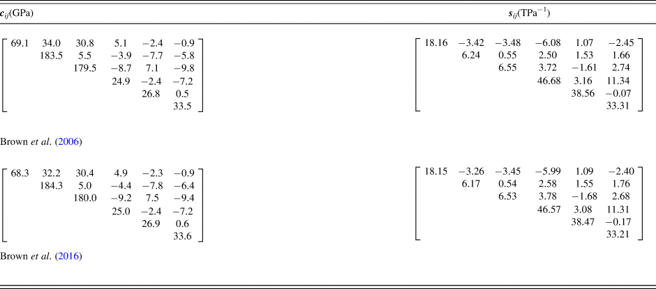
We tested both calculation routes for materials with the lowest, triclinic crystal symmetry. We calculated the compliance tensor sijkl by inversion of the stiffness tensor cijkl as published in the literature. The tested materials are: Ammonium Tetraoxalate Dihydrate (ATO), Potassium Tetraoxalate Dihydrate (KTO) (Kuppers and Siegert, Reference Kuppers and Siegert1970), Copper Sulphate Pentahydrate (Krishnan et al., Reference Krishnan, Radha and Gopal1971) and low Albite (Brown et al., Reference Brown, Abrahamson and Angel2006) and re-evaluated results for low Albite (Brown et al., Reference Brown, Angel and Ross2016) (see Table I). First, we derived in MATLAB a symbolic solution for the 4-rank tensor inverse. For each of the 21 unique elements of the compliance tensor, an (extremely long (each expression comprised in total 3051 basic operations (305 squares, 2286 products, 459 additions and 1 division))) expression was derived with the 21 independent elements of the stiffness tensor as input. Then secondly, the derived equations for the tensor inverse were first fragmented and then ported to MS-Excel for comparison with the built-in 2-rank matrix inverse function.
Single crystal elastic properties of low Albite. The compliance tensor sij is calculated by tensor inversion with an accuracy of 10−15 which is far beyond the accuracy of the input stiffness tensor cij (Brown et al., Reference Brown, Abrahamson and Angel2006, Reference Brown, Angel and Ross2016).

In all cases, the results differ only an order of magnitude of 10−15 to 10−16 which is the calculation precision of MS-Excel. Hence, one can conclude that the results are identical and there is no objection against using the faster 2-rank matrix inverse.
IV. EXPERIMENTAL
The stress measurements discussed in this paper were performed on a Malvern Panalytical X'Pert3 MRD diffractometer system with a horizontal goniometer and ½-circle cradle. The system is equipped with pre-aligned fast interchangeable (PreFIX) optics modules on the incident and diffracted beam. We used a ceramic Cu Long Fine Focus X-ray tube set to 45 kV and 40 mA for the generation of X-rays. The diffractometer radius was 320 mm.
The PreFIX optics modules for a (point focus) parallel-beam geometry were used. The incident beam module comprises an X-ray lens with an equatorial mask of 4 mm and an axial mask of 0.5 mm. The diffracted beam module comprises a parallel plate collimator with 0.27° equatorial divergence. The minimum peak resolution was about 0.4°. A Xe gas-filled proportional detector was used.
We measured symmetrical 2θ/θ scans for a series of positive and negative χ tilts such that sin2 ψ values ranging from 0 to 0.9 were covered. All available reflections (111, 200, 220, 311, 222, 400, 331, and 420) were used for single-peak stress analysis. The total experiment time was about 7 ½ hours.
To introduce residual stresses, we used a Herzog Manual Press TP20P to press a pure Cu coin (5 Euro cent) with 170 kN. Because of pressing, the topological details on the coin disappeared.
V. DISCUSSION
To test the new implementation of the Kröner method we have performed residual stress measurements on a pure Cu sample. In principle, any of the available {hkl} diffraction peaks can be chosen to measure the strain and calculate the residual stress in the sample. The stress result applies for the complete sample and there should be one consistent value. Hence, all predicted stresses should be the same. When this criterion is fulfilled the predicted X-ray Elastic Constants are the best available estimates.
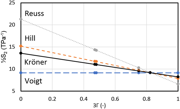
We calculated the hkl-dependent X-ray Elastic Constants S 1 and ½S 2 using the second step of the Kröner model (see Theory) in addition to estimates from the Voigt, Reuss, and Hill model (see Figure 2).
Calculated X-ray Elastic Constant ½S 2 for pure Cu as a function of the orientation parameter 3Γ (0 for 100; 1 for 111). Results of the following models are shown: Reuss (dotted line), Kröner (solid line), Hill (short dashed line) and Voigt (long dashed line).

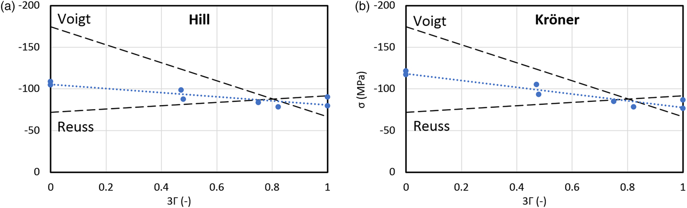
The stress results for the Hill and Kröner models are shown in Figures 3(a) and 3(b). Both models display a variation in the results. The optimum solution lies between the predictions of the Hill model and the Reuss limit (i.e. the fits is Figures 3 should have a slope of zero indicating no variation in the values of stress with respect to {hkl} diffraction peaks). Note that the Kröner model lies between the Hill model and the Voigt limit. A similar deviating result for pure Cu was observed by Murray et al. (Reference Murray, Jordan-Sweet, Bedell and Ryan2015). Their explanation for the deviation of the observed results compared to the Kroner model is the influence of plastic deformation. In our sample plastic deformation has occurred as an effect of introducing residual stresses by pressing. Though we also expect an influence of crystallographic texture or grain-shape (morphological) texture that both have been neglected in the current model calculations. In future research it has to be determined which effect is causing the observed deviations.
Predicted residual stress as a function of the orientation parameter 3Γ (0 for 100; 1 for 111): (a) Results of the Hill model and (b) results of the Kröner model. The filled circles are the experimental results for the Hill and Kröner model, respectively. The thin dotted lines are fitted trend lines to guide the eye. In both plots the limiting cases Voigt and Reuss are shown as dashed lines.

VI. CONCLUSIONS
In this article, we have discussed the implementation of the Kröner–Eshelby model for un-textured polycrystalline materials containing crystallites of any crystal symmetry. Special care is required to apply the correct multiplicative factors when the calculations are performed with matrices of rank 2 instead of tensors of rank 4. Measurements on a pure Cu coin revealed that the experimental X-ray Elastic Constants deviate significantly from the predicted values of the Kröner model. The reason could be plastic deformation and/or the influence of crystallographic or morphological texture.
Appendix A – Tensor a for Voigt, Reuss, and Hill
The tensor a for the Voigt model is defined as
 $${\bi a}_{ijkl}^{{\rm Voigt}} = ({\bar { {\bi c}}} ^{-1})_{ijkl} = {\bi S}_{ijkl} ^{{\rm Voigt}} $$
where the isotropic tensor SVoigt is obtained from elastic parameters K and G for the Voigt limit.
The tensor a for the Reuss model is defined as
 $${\bi a}_{ijkl}^{{\rm Reuss}} = {\bi s}_{ijkl}$$
The tensor a for the weighted Hill model is defined as
 $${\bi a}_{ijkl}^{w_{{\rm Hill}}} = (1-w_{{\rm Hill}})\; {\bi a}_{ijkl}^{{\rm Voigt}} + w_{{\rm Hill}}\; {\bi a}_{ijkl}^{{\rm Reuss}} $$
where the original Hill model is obtained with  $w_{{\rm Hill}} = \textstyle{1 \over 2}$ . For w Hill = 0 the Voigt limit is found and for w Hill = 1 the Reuss limit.
Appendix B – Isotropic Tensors C, S, W, and E
The isotropic tensors C, S, W, and E are defined as contravariant tensors (with indices as superscripts).
The stiffness tensor C is defined as
 $${\bi C}^{ijkl} = \lambda \delta ^{ij}\delta ^{kl} + \mu (\delta ^{ik}\delta ^{\,jl} + \delta ^{il}\delta ^{\,jk})$$
where the Lamé parameters are  $\lambda = \displaystyle{1 \over 3}(3K-2G)$ and
 $\mu = \displaystyle{1 \over 2}(2G) = G$.
The compliance tensor S is defined as
 $${\bi S}^{ijkl} = \alpha _S\delta ^{ij}\delta ^{kl} + \beta _S(\delta ^{ik}\delta ^{\,jl} + \delta ^{il}\delta ^{\,jk})$$
where the parameters are  $\alpha _S = \displaystyle{1 \over 3}\left( {\displaystyle{1 \over {3K}}-\displaystyle{1 \over {2G}}} \right)$ and
 $\beta _S = \displaystyle{1 \over 2}\left( {\displaystyle{1 \over {2G}}} \right) = \displaystyle{1 \over {4G}}$.
The Eshelby tensor E is defined as
 $${\bi E}^{ijkl} = \alpha _E\delta^{ij} \delta^{kl} + \beta _E\lpar {\delta^{ik} \delta^{\,jl} + \delta^{il} \delta^{\,jk}} \rpar $$
where the parameters are  $\alpha _E = \displaystyle{{3\lambda -2\mu} \over {15(\lambda + 2\mu )}}$ and
 $\beta _E = \displaystyle{{3\lambda + 8\mu} \over {15(\lambda + 2\mu )}}\; $.
The inverse Eshelby tensor W is defined as
 $${\bi W}^{ijkl} = \alpha _W\delta ^{ij}\delta ^{kl} + \beta _W(\delta ^{ik}\delta ^{\,jl} + \delta ^{il}\delta ^{\,jk})$$
where the parameters are  $\alpha _W = \displaystyle{{A-2B} \over 3}$,
 $A = \displaystyle{{3K + 4G} \over {3K}},\,{\rm and}\,\beta _W = B = \displaystyle{{5(3K + 4G)} \over {4(3K + 6G)}}$.