1 Introduction
The dynamics of high-Reynolds-number turbulent fountains have been the focus of considerable attention owing to their relevance to a variety of natural and industrial processes, including supply of airflows from underfloor cooling systems (Lin & Linden Reference Lin and Linden2005; Liu & Linden Reference Liu and Linden2006), refuelling of vessels (Carazzo, Kaminski & Tait Reference Carazzo, Kaminski and Tait2010), and replenishment of magma chambers (Campbell & Turner Reference Campbell and Turner1989). Following the pioneering work of Turner (Reference Turner1966), numerous studies have proposed scaling laws and models for the height of rise and the speed in the fountain and these have been tested experimentally (Hunt & Burridge Reference Hunt and Burridge2015). Fountains are often characterised in terms of the Froude number at the source,
 $Fr_{0}=u_{0}/(g_{0}^{\prime }r_{0})^{1/2}$
, where
 $r_{0}$
and
 $u_{0}$
are the source radius and velocity and
 $g_{0}^{\prime }=g{\rm\Delta}{\it\rho}_{0}/{\it\rho}$
is the buoyancy of the fluid at the source. With
 $Fr_{0}>4$
, fountains are able to entrain a significant mass of ambient fluid, and the height of rise, speed and frequency of oscillation depend primarily on the source momentum flux,
 $M=u_{0}^{2}r_{0}^{2}$
, and source buoyancy flux,
 $B=g_{0}^{\prime }u_{0}r_{0}^{2}$
. In contrast, with small source Froude number,
 $Fr_{0}<1$
, there is much less entrainment, and the properties of the fountain depend primarily on the source velocity,
 $u_{0}$
, radius,
 $r_{0}$
, and buoyancy,
 $g_{0}^{\prime }$
. The rise height of turbulent fountains is characterised by periodic oscillations of a frequency
 ${\it\omega}$
. Detailed measurements suggest that
 ${\it\omega}=f(Fr)\,u_{0}/r_{0}$
in the case
 $Fr_{0}<1$
, whereas
 ${\it\omega}\sim B/M$
in the case
 $Fr_{0}>4$
(Burridge & Hunt Reference Burridge and Hunt2013).
In explosive volcanic eruptions, two-phase fountains develop when a dense mixture of particles and gas issues from the volcano (Woods Reference Woods2010). Although theoretical models have been developed to describe the dynamics of such volcanic fountains, these models are often based on the assumption of single-phase flow, and in many cases they focus on the potential reversal of buoyancy as air is entrained and heated by the ash. One exception is the recent experimental study by Carazzo, Kaminski & Tait (Reference Carazzo, Kaminski and Tait2015), who carried out a series of experiments in which particle-laden hot air was supplied to the base of a room containing cooler air. They explored the partitioning of the particles as some fell from the flow, while the remaining mixture of the particles and hot air became buoyant. The experimental results were compared with the predictions of a numerical model of a rising fountain with reversing buoyancy. However, there is more to learn about the dynamics of particle-laden fountains, which, as well as being related to volcanic eruptions, are of fundamental interest for industrial fluidisation-type processes in which jets of fluid are used to suspend particles.
The purpose of this work is to present a series of experiments in which a jet of fresh water laden with heavy particles is supplied to the base of a tank containing fresh water, and to compare the dynamics of such a particle-laden fountain with those of an equivalent salt fountain. We show that the ratio
 $U$
of the particle fall speed to the characteristic fountain speed distinguishes between conditions in which the particle-laden flow behaves effectively as a single-phase fluid,
 $U\ll 1$
, and conditions in which the two phases separate owing to particle fallout,
 $U>1$
. Also, using new measurements, we recognise that
 $Fr\approx 1$
at the mean height of a single-phase fountain, and so the amplitude of the oscillations of the height of the fountain,
 ${\rm\Delta}h$
, is similar to the fountain radius at the mean height of the fountain. In the limit
 $U\ll 1$
, this leads to a picture of fountain oscillations being controlled by the periodic accumulation and collapse of fluid at the fountain top, where
 $Fr<1$
. In contrast, in the limit
 $U>1$
, the particles separate from the fountain fluid while
 $Fr>1$
, and since the fluid still has a significant upward momentum, it continues upwards.
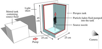
Schematic diagram of the experimental set-up.

2 Experiments
We carried out a series of experiments in a tank of dimension
 $25~\text{cm}\times 25~\text{cm}\times 45~\text{cm}$
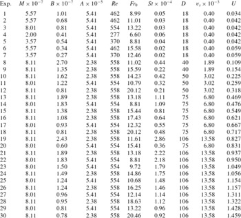
(figure 1). The tank was filled with fresh water, and a source nozzle was placed in the centre of its base. To observe the impacts of different source conditions, two round nozzles of diameter 5.5 and 8.3 mm were used in the experiments (see table 1). During each experiment, one of the nozzles was connected to a stirred tank containing a suspension of water and silicon carbide particles (Washington Mills). The suspension of particles used in each experiment was monodisperse; however, particles of different sizes were used in different experiments to observe the impacts of different particle fall speeds. Table 1 shows that the diameter
 $D$
of the particles used in the experiments ranged between 18 and
 $106~{\rm\mu}\text{m}$
. Five settling experiments were run to measure the fall speeds of these particles in water, using the method described in Mingotti & Woods (Reference Mingotti and Woods2015). These experiments indicated that particles of different diameters settled at different speeds, ranging between 0.4 and 13.6 m
 $\text{m}~\text{s}^{-1}$
(table 1), in good agreement with the range of expected Stokes terminal velocities. In all experiments, the fall speed of the particles was much smaller than the speed of the fountain fluid at the source (see table 1,
 $St\ll 1$
). Consequently, particles rapidly acquired the flow speed and behaved like tracers in the fluid in the region above the source.
The particle-laden fluid was supplied to the experimental tank using a peristaltic pump (Watson Marlow) at a number of different flow rates, ranging between 4 and
 $8~\text{cm}^{3}~\text{s}^{-1}$
. In our experiments, the outflow from the nozzle rapidly became turbulent; however, in the pipe feeding the nozzle, the flow might not be fully turbulent and this might have an impact on the source momentum flux (Baines, Turner & Campbell Reference Baines, Turner and Campbell1990). Following Baines et al., whose experiments had similar source conditions to the present study, we assumed the flow through the nozzle to be laminar, and estimated the source momentum flux by calculating the equivalent momentum of a flow with constant velocity across a hole with diameter 0.83 times the nozzle diameter. However, in all figures, error bars are shown to include the possibility that the flow in the nozzle is in fact turbulent. We also note that in the majority of our experiments, the Froude number at the source was in the range
 $Fr_{0}\approx 6{-}20$
and the Reynolds number,
 $Re\approx 460{-}560$
(table 1). This is consistent with the motion of the fountain fluid becoming turbulent on leaving the source and the motion being controlled by the momentum and buoyancy fluxes,
 $M$
and
 $B$
(Williamson et al.
Reference Williamson, Srinarayana, Armfield, McBain and Lin2008).
Conditions of the particle fountain experiments. We let
 $M$
(
 $\text{m}^{4}~\text{s}^{-2}$
) denote the momentum flux at the source, while
 $B$
(
 $\text{m}^{4}~\text{s}^{-3}$
) is the downward buoyancy flux at the source,
 $A$
(
 $\text{m}^{2}$
) is the cross-sectional area of the nozzle,
 $D$
(
 ${\rm\mu}\text{m}$
) and
 $v_{s}$
(
 $\text{m}~\text{s}^{-1}$
) are the diameter and settling speed of the particles and
 $U=v_{s}M^{1/4}B^{-1/2}$
is the ratio between the particle fall speed and the characteristic fountain speed given by (2.1).
 $Re$
,
 $Fr_{0}$
and
 $St$
are the Reynolds, Froude and Stokes numbers associated with the particle-laden flow at the source (Williamson et al.
Reference Williamson, Srinarayana, Armfield, McBain and Lin2008; Hunt & Burridge Reference Hunt and Burridge2015).

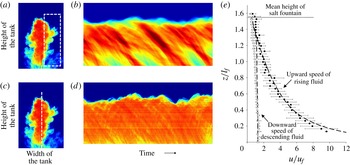
(a) False colour image of a photograph of a typical fountain. For each photograph captured during an experiment, we measured the instantaneous profile of light attenuation along the fountain centreline, as well as the horizontally averaged profile in the region near the flanks of the fountain (shown by the dashed white lines in (c) and (a) respectively). We then plotted the time series of these profiles (d and b respectively). The inclined lines across which the light intensity changes in these figures illustrate the upward and downward motion of parcels of dyed fluid in the tank. We used the Hough transform to measure the gradient of the upward- and downward-sloping lines in these images, and thereby estimate the time-averaged velocities of the rising and descending fluid. In (e), solid and open circles are used to plot the average velocities that were measured during our experiments (table 1), scaled by the characteristic fountain speed
 $u_{f}$
(2.1).

The tank was backlit using a light sheet (LightTape by Electro-LuminX Lighting Corp.). During an experiment, the light emitted by the sheet was attenuated across the tank containing particle-laden fluid. We typically used particle concentrations of order 1–
 $10~\text{g}~\text{l}^{-1}$
at the source: within this range of concentrations, light attenuation could be detected using a Spark SP-5000M-USB camera located on the opposite side of the tank (figure 1). To observe the motion of the fountain fluid over time, we captured images at a frequency of 200 Hz. For calibration purposes and to test our experimental results with the existing models (including those given by Mizushina et al.
Reference Mizushina, Ogino, Takeuchi and Ikawa1982, Bloomfield & Kerr Reference Bloomfield and Kerr2000 and Burridge & Hunt Reference Burridge and Hunt2013), we repeated some of the experiments listed in table 1 using the same momentum and buoyancy fluxes, but with a saline solution as the source fluid in order to generate a single-phase fountain. Photographs captured during each experiment were analysed to measure: (i) the speed of the rising and of the descending fluid in the fountain, (ii) the time-averaged mean and maximum fountain heights, and (iii) the frequency and the amplitude of oscillations in the fountain height.
Depending on the volume flux and on the bulk density of the source fluid, the fountains in our experiments were typically 4–10 cm tall and 3–7 cm wide, and since the reservoir used for the experiments was much larger (see figure 1), we expect that there were no significant confinement effects.
2.1 Salt fountains
Figure 2 shows how the speed of the fountain fluid was measured in an experiment. For each photograph captured during the experiment, we initially considered a portion of the image near the outer flank of the fountain (figure 2
a), and measured the horizontally averaged profile of light attenuation in this region. We show a time series of light attenuation profiles in figure 2(b). In this image, parcels of saline fluid that descend from the top of the fountain towards the base of the tank lead to a descending front across which there is a change in the light intensity. Following Rocco & Woods (Reference Rocco and Woods2015), we used the Hough transform as available in Matlab to identify these fronts, calculate their gradient and thereby estimate the speed of the descending parcels of saline fluid as a function of the vertical distance
 $z$
above the source. By calculating the speed of many such fronts, we can estimate the average speed as a function of height above the source (white circles in figure 2
e). We repeated the process to measure the upward speed of the saline fluid in the core of the fountain by plotting a time series of the light attenuation on the vertical axis of the fountain (figure 2
c,d). By averaging the gradient of the forward-sloping lines in this image, we estimated the mean velocity profile in the centre of the fountain (black circles in figure 2
e). We note that in plotting the experimental data, we have scaled the speed with the scaling for the fountain speed based on the buoyancy and momentum flux,
 $u_{f}$
, where
 $$\begin{eqnarray}u_{f}=B^{1/2}M^{-1/4},\end{eqnarray}$$
where
 $B$
and
 $M$
are the buoyancy and momentum flux at the source respectively (see table 1). Within experimental error, the data seem to follow a universal curve using this scaling, and this is consistent with the picture of a turbulent fountain for which
 $Fr\gg 1$
, as proposed by Turner (Reference Turner1966). Figure 2(e) also shows that the measured velocity profiles are in good accord with data collected by Mizushina et al. (Reference Mizushina, Ogino, Takeuchi and Ikawa1982), and with the predictions of the integral model of a fountain proposed by McDougall (Reference McDougall1981) and Bloomfield & Kerr (Reference Bloomfield and Kerr2000) (dashed lines). In plotting figure 2(e), we scaled heights with the characteristic length scale
 $l_{f}$
given by
 $$\begin{eqnarray}l_{f}=M^{3/4}B^{-1/2}.\end{eqnarray}$$
Our experimental results indicate that the top height
 $h_{t}$
and the mean height
 $h_{m}$
of a single-phase fountain scale with
 $l_{f}$
, with constants of proportionality
 ${\it\lambda}_{t}=1.68\pm 0.05$
and
 ${\it\lambda}_{m}=1.56\pm 0.04$
respectively, in accord with Turner (Reference Turner1966) and Hunt & Burridge (Reference Hunt and Burridge2015) in the range
 $20>Fr>6$
. By injecting a number of pulses of dyed fluid at the source of a transparent salt fountain, we observed the rising fluid in the core of the fountain and found that at the mean height of the fountain,
 $h_{m}$
, the inner fountain radius is
 $r(h_{m})=(0.155\pm 0.007)h_{m}$
, in accord with Mizushina et al. (Reference Mizushina, Ogino, Takeuchi and Ikawa1982). Using a Fourier transform on a time series of the rise height of our salt fountains, we determined that the dominant frequency of oscillations scales as
 ${\it\omega}_{salt}=(0.48\pm 0.02)u_{f}/l_{f}$
in accord with Turner (Reference Turner1966) and Burridge & Hunt (Reference Burridge and Hunt2013).
(a) Height of rise, (b) frequency and (c) amplitude of the oscillations in particle-laden fountains relative to those in salt fountains, for a range of different particle settling speeds relative to the fountain speed. In (a), closed circles are used to illustrate the ratio between the particle fall speed and the fountain speed, assuming the flow in the nozzle is laminar, while for comparison open circles illustrate the same ratio if we assume that the flow in the nozzle is turbulent (Baines et al. Reference Baines, Turner and Campbell1990). In (b,c), we assume the flow is laminar in the nozzle, but include horizontal error bars to illustrate the uncertainty associated with the source condition.

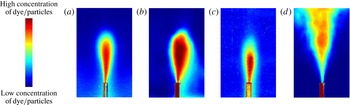
Time average of (a,c) the particles and (b,d) the dyed fluid in a particle-laden fountain, as obtained for the case (a,b)
 $U=0.32$
and (c,d)
 $U=1.32$
(experiments 12 and 28 respectively, see table 1). In (a,c) the fluid was undyed, so that the images reflect the particle load, while in experiments (b,d) the source fluid was dyed, so the images reflect the concentration of the fluid, integrated through the field of view of the fountain.

2.2 Particle fountains
Having tested our experimental approach, we carried out a series of particle fountain experiments. We systematically varied the particle load and size, and the source mass and momentum flux so that the ratio of the fall speed of the particles relative to the characteristic fountain speed,
 $U=v_{s}/u_{f}$
, took values in the range 0.03–1.5 (see table 1). In figure 3(a) we illustrate the variation with
 $U$
of the mean height of rise of the particle fountains,
 $h_{m}$
, as a fraction of the height of the corresponding single-phase fountains. In figure 3(b,c) we illustrate the frequency
 ${\it\omega}$
and the amplitude
 ${\rm\Delta}h$
of the oscillations at the top of the particle fountains, again shown as a fraction of the values for the equivalent salt fountains. It is seen that for
 $U<0.1$
, the particle fall speed is so small compared with the fountain speed that the particle-laden fluid behaves essentially as a single-phase fluid. In this limit, the height of rise of the fountain and the amplitude of the oscillations scale with
 $l_{f}$
, while the frequency of the oscillations scales as
 $B/M=u_{f}/l_{f}$
.
However, our experiments indicate that for
 $U>0.4{-}0.5$
, the mean height of rise of a particle fountain is smaller than that of the equivalent salt fountain (figure 3(a)). This happens because for
 $U>0.5$
the particles separate from the fountain fluid and fall out. Figure 4 illustrates the time-averaged distributions of the particles and of the fountain fluid in two experiments with different ratios of particle speed to fluid speed (
 $U_{1}=0.32$
and
 $U_{2}=1.32$
respectively, see table 1). To make this figure, we repeated each experiment using clear and then dyed particle-laden water as the source fluid, so that the fate of the particles and the fluid could be independently tracked. Each image in the figure represents the time-averaged distribution of the particles/fluid over 30 s, and uses false colours to illustrate the different concentrations of particles/dye in the tank during this time. Figure 4(a,b) shows that for
 $U<0.5$
both the small particles and the fountain fluid rose to a maximum height and then collapsed as a bulk to the floor. It is seen that the two time-averaged images overlap considerably although the fluid is somewhat more dispersed radially than the particles. In contrast, figure 4(c,d) shows that for
 $U>0.5$
the larger particles remained in a close neighbourhood of the fountain centreline as they cascaded down to the floor, while the fountain fluid continued to rise above the particle zone driven by its momentum. This is not a conventional fountain collapse, but a process of separation of the fluid and particles.
For each experiment in the separated flow regime, we used the data provided by Mizushina et al. (Reference Mizushina, Ogino, Takeuchi and Ikawa1982), which are in good agreement with the predictions of the model developed by Bloomfield & Kerr (Reference Bloomfield and Kerr2000), to estimate the upward speed of the fluid in the core of the fountain at different levels above the source nozzle (see figure 2
e). We then identified the height at which this speed matches the fall speed of the particles,
 $v_{s}$
, and we include this theoretical curve in figure 3(a) as a function of
 $U$
(red dashed line). It is seen that the heights of rise of the particles in the separated flow regime are similar to this model prediction, and this suggests that particles do not rise beyond the point at which their fall speed equals the ascent speed of the rising flow in the fountain.
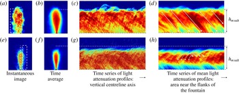
On reaching this level, the particles continuously fall out and settle to the floor, and so the oscillations that are characteristic of the top of a single-phase fountain are suppressed. Indeed, figure 3(c) shows that as
 $U$
increases beyond the value
 $U\approx 0.1$
, the amplitude of the oscillations at the top of the particle fountain rapidly decreases compared to that of the corresponding salt fountains, while the frequency of the oscillations increases (figure 3
b). Our experimental results suggest that there is a smooth transition between the pseudo-single-phase flow regime and the separated flow regime as
 $U$
increases from
 $0.1$
to 0.4–0.5. Over this range, the mean heights of the particle fountains decrease from
 $h_{m,salt}$
to
 $h_{m,salt}-{\rm\Delta}h$
(figure 3
a), where
 ${\rm\Delta}h$
is the amplitude of the oscillations of the equivalent salt fountains.
3 Discussion
In order to build insight into why for
 $U>0.5$
particle-laden fountains do not appear to exhibit the strong oscillatory behaviour seen in purely saline fountains, we have measured some further properties of the oscillations in saline fountains and fountains laden with very small particles (
 $U\ll 1$
). In particular, we have combined (i) new measurements of the inner radius,
 $r$
, and the speed,
 $u$
, of the fountain at the mean height
 $h_{m}$
with (ii) an estimate of the buoyancy of the fountain fluid at this height using a dimensionless model for the buoyancy in a fountain based on experimental measurements as reported by Mizushina et al. (Reference Mizushina, Ogino, Takeuchi and Ikawa1982), to determine the Froude number at the mean height of rise,
 $Fr(h_{m})$
. We have found that for single-phase fountains the local Froude number is given by
 $$\begin{eqnarray}Fr(h_{m})=\frac{u(h_{m})}{[g^{\prime }r(h_{m})]^{1/2}}=1.06\pm 0.12\end{eqnarray}$$
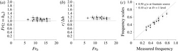
as plotted in figure 5(a).
In their experimental study, Burridge & Hunt (Reference Burridge and Hunt2013) measured the frequency of the oscillation of weak saline fountains for which the source condition was
 $Fr_{0}=1$
, and found
 ${\it\omega}=\left(0.10\pm 0.028\right)\,u/r$
, where
 $u$
and
 $r$
are the speed and the radius of the fountain fluid at the source. They argued that this is distinct from the oscillations that develop in a fountain for which
 $Fr_{0}\gg 1$
. However, if we apply the Burridge–Hunt result, but using as source conditions the measured speed, buoyancy and radius of the fountain fluid at the height
 $h_{m}$
, where we have shown that
 $Fr\approx 1$
, then we find that the predicted frequency is in very good accord with our observations (see the open circles in figure 5
c). Predictions based on the classical scaling for fountains with
 $Fr_{0}>5$
are also in good accord with the observations: in figure 5(c) we use solid circles to plot the expected frequencies of oscillation
 ${\it\omega}=\left(0.5\pm 0.103\right)\,g_{0}^{\prime }/u_{0}\sim B/M$
, in which
 $g_{0}^{\prime }$
and
 $u_{0}$
are the buoyancy and the speed of the fluid at the source of the fountain (Turner Reference Turner1966).
(a) Estimate of the Froude number at a height
 $h_{m}$
above the source in our experiments. (b) Experimental measurements of the ratio between the fountain inner radius
 $r(h_{m})$
and the amplitude of the oscillations in the fountain rise height
 ${\rm\Delta}h$
. (c) The frequencies of the oscillations that were measured during the experiments (Hz) are compared with: (i) the expected frequencies estimated using the classic scaling for turbulent fountains based on the source conditions (black circles), and (ii) the expected frequencies estimated using the scaling for weak fountains given by Burridge & Hunt (Reference Burridge and Hunt2013) and the properties of the flow measured at the height
 $h_{m}$
above the source (white circles).

Fountains laden with (a–d) small and (e–h) large particles (experiments 3 and 29 in table 1). For each experiment, we plot: (a,e) an image that illustrates the distribution of particles in the tank at a given time during the experiment (cf. salt experiment depicted in figure 2 a); (b,f) a time-averaged image showing the mean distribution of particles during 30 s; (c,g) a time series of the vertical profiles of light attenuation along the centreline (cf. salt experiment depicted in figure 2 d); and (d,h) a time series of the horizontally averaged profiles of light attenuation in the region near the flanks of the fountain (cf. salt experiment depicted in figure 2 b). Panels (c,d) show that when the fountain is laden with small particles, dense parcels of particle-laden fluid accumulate at its top and collapse periodically; however, (g,h) show that when the fountain is laden with large particles, these particles fall out and sediment. While settling, some are entrained and resuspended. Ballistic trajectories.

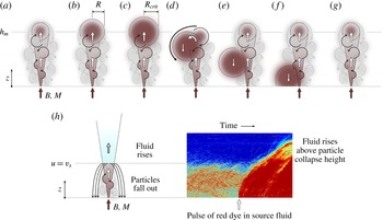
Cartoons illustrating the different mechanisms of collapse of a fountain laden with smaller (a–g) or larger particles (h).

The coincidence of the experimental data and the scaling for the frequency based on the fountain properties at
 $Fr=1$
suggests that oscillations in a salt fountain or in a fountain laden with small particles (
 $U\ll 1$
) arise from a balance between the supply of new dense fluid and the convective settling of this fluid at the top of the fountain, in the region
 $Fr<1$
(see figures 6
d and 7). Fluid that is supplied by the fountain with
 $Fr=1$
at
 $z=h_{m}$
will continue to rise to the maximum height
 $h_{t}$
prior to exhausting its kinetic energy. A cloud of fountain fluid will then build up at the top of the fountain (figure 7
a–c), and it will gradually begin to descend to the floor. We expect that once the downward volume flux of this cloud exceeds the volume flux supplied from the fountain, then a discrete parcel of fluid will descend from the top of the fountain (figure 7
c–f), and the cycle will repeat. If we let
 $R$
denote the effective radius of one such parcel of dense fluid, modelled as a sphere, then we expect that this radius will increase over time according to
 $$\begin{eqnarray}\frac{\text{d}}{\text{d}t}\left(\frac{4}{3}{\rm\pi}R^{3}\right)=Q_{f},\end{eqnarray}$$
where
 $$\begin{eqnarray}Q_{f}\sim {\it\gamma}M^{5/4}B^{-1/2}\end{eqnarray}$$
is the volume flux supplied at the top of the fountain. The convective fall speed of the growing parcel of dense fluid scales as
 ${\it\alpha}(g^{\prime }R)^{1/2}$
where
 ${\it\alpha}$
is a constant of proportionality that we estimate as
 ${\it\alpha}=0.6\pm 0.15$
from our experiments (e.g. figure 2
e). When multiplied by the horizontal cross-sectional area, we estimate that the parcel has downward volume flux
 ${\it\alpha}{\rm\pi}(g^{\prime }R^{5})^{1/2}$
, which exceeds the supply rate from the fountain
 $Q_{f}$
when
 $R>R_{crit}$
where
 $$\begin{eqnarray}{\it\alpha}(g^{\prime }R_{crit})^{1/2}{\rm\pi}R_{crit}^{2}=Q_{f}.\end{eqnarray}$$
At this stage, the volume of dense fluid may fall to the base of the tank (figure 7
d–f), and a new volume will start developing (figure 7
g). Using a combination of (3.2)–(3.4), we calculate that the period
 $t$
between two oscillations in the fountain rise height is given by
 $$\begin{eqnarray}t=\frac{1}{{\it\omega}}=\frac{4}{3}\frac{{\it\gamma}^{4/5}}{{\rm\pi}^{1/5}{\it\alpha}^{6/5}}\frac{M}{B},\end{eqnarray}$$
and using the speed and frequency data that we measured in our experiments (figure 3
a and b respectively), we estimate that
 ${\it\gamma}=1.07\pm 0.26$
.
In the case of separated flow,
 $U>0.5$
, the particle fall speed is sufficiently large that the Froude number of the fountain exceeds unity at the maximum height reached by the particles (figure 6
e–h). As a result, once the particles have fallen out, the fluid remaining in the fountain continues to rise (see figure 7
h), and the mechanism by which dense fluid accumulates at the top of the fountain is no longer effective. The small-amplitude, high-frequency oscillations seen in figure 6(g,h) may be associated with clustering of the particles, perhaps arising from resuspension of particles by the rising fluid.
Although our experiments are relatively simple compared to the fountain that forms during an explosive volcanic eruption (cf. Woods Reference Woods2010), it is nonetheless of interest to estimate the range of particle sizes for which
 $U$
is of order 1 in such an event. With source velocities of order 100–
 $150~\text{m}~\text{s}^{-1}$
, source radii of order 100–300 m and initial density in the range 1–
 $10~\text{kg}~\text{m}^{-3}$
, we estimate that
 $M\sim 10^{8}$
 $\text{m}^{4}~\text{s}^{-2}$
and
 $B\sim 10^{7}~\text{m}^{4}~\text{s}^{-3}$
, leading to a characteristic volcanic fountain speed of order
 $u_{f}\sim 30{-}50~\text{m}~\text{s}^{-1}$
. Depending on the density of the fountain, this speed matches the fall speed of pumice particles with size of order 5–50 cm (Woods Reference Woods1988). Although noting the simplicity of the model, which neglects the effects of the heating of air entrained into the fountain, which can lead to a reversal in buoyancy of the fountain, this scaling suggests that particles larger than 5–50 cm are likely to fall out of a fountain prior to reaching the top of the fountain. Smaller particles, however, may continue to rise with the fountain fluid, and in some cases may then become buoyant and form a convecting eruption column. We plan to develop this work further to consider some of the additional processes controlling the dispersal of different sized particles in these volcanic flows.
4 Conclusions
We have studied the dynamics of particle-laden fountains, produced by the injection of a mixture of particles and water into a tank filled with water. In the case
 $U<0.1$
, the fountain behaves as a single-phase fountain and the flow rises to a mean height at which
 $Fr\approx 1$
. The fountain oscillates about this mean height as discrete volumes of fluid build up and then fall to the ground. The frequency of the oscillations coincides with the frequency of oscillations of a fountain issuing from a source with
 $Fr=1$
located at a height
 $h_{m}$
above the original source, suggesting that the oscillations are controlled by the upper region of the fountain where
 $Fr<1$
. In contrast, when
 $U>0.4{-}0.5$
, we have found that for source Froude numbers in the range
 $6<Fr_{0}<20$
the particles fall out of the fountain below the height at which
 $Fr=1$
. As the particles separate from the flow, the fluid continues rising; this suppresses the development of oscillations at the maximum height reached by the particles, in contrast to the case
 $U<0.1$
, which is analogous to a single-phase fountain.
Acknowledgement
This work has been funded through the BP Institute, EPSRC and Hughes Hall, Cambridge. We gratefully acknowledge the technical assistance of A. Pluck, and the constructive comments of three anonymous referees.