2. Experimental and numerical methods

2.1. Experimental set-up and parameters

The experimental apparatus was designed for high-resolution flow field measurements in rotating RBC (Chong et al. Reference Chong, Shi, Ding, Ding, Lu, Zhong and Xia2020; Shi et al. Reference Shi, Lu, Ding and Zhong2020; Ding et al. Reference Ding, Chong, Shi, Ding, Lu, Xia and Zhong2021). Here, we present only its essential features. The bottom plate of the convection cell was made of oxygen-free, high-conductivity copper. Its bottom side was covered uniformly by parallel straight grooves. A main heater made of resistance wires was epoxied into the grooves. Seven thermistors were installed into the bottom plate, at vertical distance 3.5 mm from the top surface of the plate. The main heater was operated in a digital feedback loop in conjunction with these thermistors to hold the bottom-plate temperature as a constant with a stability of a few millikelvins. For the purpose of flow visualization, we used a top plate made of a 5 mm thick sapphire disc. A thermal bath that contained circulating coolant was constructed over the sapphire plate and regulated its temperature. During the experiment, the temperature fluctuation of the top plate was within 0.005 K.

The temperature difference between the bottom plate and the ambient air may induce thermal perturbations to the experiment. To eliminate this temperature difference, a bottom adiabatic shield was installed under the bottom plate. This thermal shield was covered by a bottom-shield heater, with a thermistor located at the centre of the shield. A second auxiliary heater was wound around the periphery of the shield, and the local temperature there was measured by a second thermistor. Both heaters worked in conjunction with their relevant thermistors to maintain the bottom-shield temperature the same as the bottom-plate temperature.

In between the top and bottom plates was a cylindrical sidewall made of plexiglas with a thickness of 3 mm. Thermal protection towards the sidewall was provided by a separate thermal side shield. It was a thin cylindrical ring made of aluminium, with a spiral aluminium tube wound on its outer surface. A circulating flow of coolant passed through the aluminium tube kept the side-shield temperature at the mean fluid temperature. Most of the spatial volume in between the thermal shields and the convection cell was filled with low-density open-pore foam to prevent convective air flows. The aforementioned two coolant circuits were brought into the rotary table through a rotary union. It was a four-passage feed through equipped with a slip ring for electrical leads. The rotary table rotated clockwise driven by an electric servo-motor. All components of the convection cell were installed on the rotary table.

In the present study, we used two cylindrical cells with an inner diameter $D_{0}=240$ mm, and fluid height $H=63.0$ (120.0) mm, yielding the aspect ratio $\varGamma _{a}=D_{0}/H=3.8$ (2.0). Deionized water was the working fluid, with a constant Prandtl number ${Pr}=\nu /{\kappa }=4.38$. The experiment was conducted in the range $2.0\times 10^7\le Ra\le 2.7\times 10^8$ of the Rayleigh number ${Ra}={\alpha }g\,{{\rm \Delta} }T\,H^3/{\kappa }{\nu }$ (where $\alpha$ is the isobaric thermal expansion coefficient, $g$ is the acceleration of gravity, ${\rm \Delta} T$ is the applied temperature difference, $\kappa$ is the thermal diffusivity, and $\nu$ is the kinematic viscosity). For each dataset with the same $Ra$, all measurements were made at constant ${\rm \Delta} T$, with $\varOmega$ varying from 0.31 to 5.0 rad s$^{-1}$. The Ekman number ${Ek}=\nu /(2{\varOmega }H^2)$ spanned $1.7\times 10^{-5}\le Ek\le 2.7\times 10^{-4}$. The Froude number ${Fr}={\varOmega }^2D_{0}/2g$ was within $1.2\times 10^{-3}\le Fr\le 0.31$. 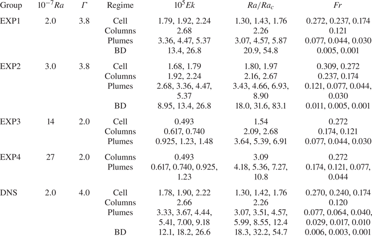The convection in the experiment is assured by examining the reduced number $Ra/Ra_c$ greater than 1, where $Ra_c=(8.7-9.63\,Ek^{1/6})\,Ek^{-4/3}$ (Niiler & Bisshopp Reference Niiler and Bisshopp1965) is the critical value for the onset of convection in a horizontally infinitely large system. More information about various parameter regimes is reported in table 1.

Table 1.

Parameters of all experimental runs. Results for $\varGamma =3.8, 2.0$ are acquired from convection cells with $H=63, 120$ mm, respectively. The dynamical regimes are determined based on Julien et al. (Reference Julien, Rubio, Grooms and Knobloch2012), Kunnen (Reference Kunnen2021) and Lu et al. (Reference Lu, Ding, Shi, Xia and Zhong2021). BD is an abbreviation for the buoyancy-dominated regime.

We conducted measurements of the horizontal velocity field ($u_x, u_y$) using a particle image velocimetry system installed on the rotary table. A thin light sheet powered by a solid-state laser illuminated the seed particles in a horizontal plane at fluid height $z=H/4$. Images of the particle were captured through the top sapphire window by a high-resolution camera ($2456\times 2058$ pixels). Two-dimensional velocity fields were extracted by cross-correlating two consecutive particle images. Each velocity vector was calculated from an interrogation window ($32\times 32$ pixels), with $50\,\%$ overlap of neighbouring sub-windows to ensure sufficient resolution of the velocity field (Westerweel, Elsinga & Adrian Reference Westerweel, Elsinga and Adrian2013; Shi et al. Reference Shi, Lu, Ding and Zhong2020). Thus we obtained $154\times 129$ velocity vectors on each frame, reaching resolution 2.0 mm for the velocity field. We identify the vortices through a two-dimensional $Q$-criterion. Considering the quantity $Q=({\rm Tr}\,\boldsymbol {A})^2-4\,{\rm det}\, \boldsymbol {A}$ with the velocity gradient tensor $\boldsymbol {A}=[\partial (u_x,u_y)/\partial (x,y)]$, we define the vortex centre as the minimum of $Q$ within a vortex region satisfying $Q<-Q_{std}$. Here, $Q_{std}$ is the standard deviation of $Q$ over the measured area $r\le D_{0}/4$ (Chong et al. Reference Chong, Shi, Ding, Ding, Lu, Zhong and Xia2020; Ding et al. Reference Ding, Chong, Shi, Ding, Lu, Xia and Zhong2021). We adopt the method of vortex tracking introduced in Ding et al. (Reference Ding, Chong, Shi, Ding, Lu, Xia and Zhong2021) to obtain vortex trajectories.

2.2. Numerical method

In the direct numerical simulations (DNS), we solved the three-dimensional Navier–Stokes equations within the Boussinesq approximation:

(2.1)$$\begin{gather} \frac{{\rm D}\boldsymbol{u}}{{\rm D} t}={-}\boldsymbol{\nabla}P+\left(\frac{Pr}{Ra}\right)^{1/2}{\nabla}^2\boldsymbol{u}+{\theta}\hat{z}+ \left(\frac{Pr}{Ra\,Ek^2}\right)^{1/2}\boldsymbol{u}\times \hat{z}-\frac{2r\,Fr}{D}\,{\theta}\hat{r}, \end{gather}$$

(2.2)$$\begin{gather}\frac{{\rm D}{\theta}}{{\rm D} t}=\frac{1}{(Ra\,Pr)^{1/2}}\,{\nabla}^2{\theta}, \end{gather}$$

(2.3)$$\begin{gather}\boldsymbol{\nabla}\boldsymbol{\cdot}\boldsymbol{u}=0. \end{gather}$$

Here, $\boldsymbol {u}$ is the fluid velocity, and $\theta$ and $P$ are the reduced temperature and pressure.

Equations (2.1)–(2.3) were non-dimensionalized using $H$, ${{\rm \Delta} }T$ and the free-fall velocity $U_{f}=\sqrt {\alpha g\,{\rm \Delta} T\,H}$. The top (bottom) plate was isothermal with temperature $\theta _{t}=-0.5$ ($\theta _{b}=0.5$), and the sidewall was thermally insulated. As for the momentum boundary condition, all boundaries were no-slip. These equations were solved using the multiple-resolution version of CUPS (Kaczorowski & Xia Reference Kaczorowski and Xia2013; Chong, Ding & Xia Reference Chong, Ding and Xia2018), which was a fully parallelized DNS code based on a finite-volume method with fourth-order precision. To improve computational efficiency without any sacrifice in precision, we used a multiple-resolution strategy. The grid resolutions along the radial, azimuthal and vertical directions were $140\times 384\times 160$ for the momentum and pressure fields, and $280\times 768\times 160$ for the temperature field. We examine the ratios between the vertical grid spacing and the local Kolmogorov and Batchelor length scales. The maximum value of these two ratios for all cases is about 1.2, and for most of the cases, these two ratios are well below unity. Additionally, the thickness of the Ekman boundary layer decreases as $Ek$ decreases. We ensured that there were no fewer than 11 grid points within the Ekman layer even for the smallest $Ek$ of the present work, to resolve the Ekman boundary layer sufficiently. The simulations were performed in a cylindrical domain with $\varGamma _{a}=4$, ${Ra}=2.0\times 10^{7}$, ${Pr}={\nu }/{\kappa }=4.38$ and $1.3\le {Ra/Ra_c}\le 55$.

3. Vortex spatial distribution

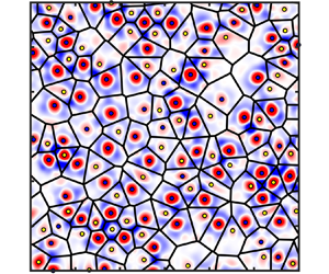
In the rotating RBC, the spatial distribution and organization of the convective vortices depend sensitively on the strength of rotation and buoyancy. To demonstrate the distribution of the columnar vortices, we present in figure 1 Voronoi diagrams of the vortex centres for two reduced Rayleigh numbers, $Ra/Ra_{c}=8.90$ and 2.67. The background colour of these diagrams represents the distribution of the $Q$ field, where vortices are shown in reddish colour, and the bluish areas in between indicate regions of high flow strain. We see that under weak rotations, the vortices appear to be located randomly with a broad size distribution for $Ra/Ra_{c}=8.90$. The Voronoi cells become smaller on average but seemingly have an even size distribution for rapid rotations ($Ra/Ra_{c}=2.67$).

Figure 1.

Spatial distribution of the vortices for (a) weakly rotating convection and (b) rotation-dominated convection. The solid line network constitutes the Voronoi diagram of the vortex centres. The background colouration represents the distribution of the quantity $Q/Q_{std}$, with blue (yellow) dots denoting the centres of anticyclones (cyclones). Experimental results for $Ra=3.0\times 10^7$ and for (a) $Ra/Ra_{c}=8.90$ and(b) $Ra/Ra_{c}=2.67$.

In the following analysis, we consider the probability density functions (PDFs) of Voronoi cell area of the vortices. It has been shown that for randomly distributed entities in $d$-dimensional space ($d\le 3$), the PDF of their Voronoi areas (volumes) normalized by the mean is the standard $\varGamma$ distribution (Ferenc & Néda Reference Ferenc and Néda2007; Tagawa et al. Reference Tagawa, Mercado, Prakash, Calzavarini, Sun and Lohse2012):

(3.1)\begin{equation} P(x)=\frac{[(3d+1)/2]^{(3d+1)/2}}{\varGamma[(3d+1)/2]}\,{x}^{{(3d-1)}/{2}}\exp({-[(3d+1)/2]x}). \end{equation}

Here, the denominator is a $\varGamma$ function. For two-dimensional distributions ($d=2$), we have $P_2(x)=7^{7/2}2^{-7/2}x^{5/2}\exp ({-7x/2})/{\varGamma }(7/2)$. The Voronoi diagram offers a qualitative scheme to describe the spatial distributions of entities in densely populated systems (Ferenc & Néda Reference Ferenc and Néda2007; Tagawa et al. Reference Tagawa, Mercado, Prakash, Calzavarini, Sun and Lohse2012). For example, the clustering effect of particles in turbulence leads to an increase of the standard deviation of the scaled Voronoi volumes of the particles, and thus the PDF of the Voronoi volumes deviates from the standard $\varGamma$ distribution (Tagawa et al. Reference Tagawa, Mercado, Prakash, Calzavarini, Sun and Lohse2012).

Figure 2(a) shows the PDFs of the Voronoi cell areas $A$ of the vortices normalized by the mean value $P(A/{\langle }A{\rangle })$. We see that for $Ra/Ra_{c}=83.09$, $P(A/{\langle }A{\rangle })$ follows closely the standard $\varGamma$ distribution $P_2(x)$. With increasing rotation rates (decreasing $Ra/Ra_{c}$), the PDFs of the Voronoi cell area show behaviour different from that of the standard $\varGamma$ distribution. We see that the PDFs have a smaller possibility for very large and small cells than for random distributed ones, but a larger probability for $A/{\langle }A{\rangle }\approx 1$. These results suggest that the vortices are indeed randomly distributed for a sufficiently large $Ra/Ra_{c}$. The size distribution of the Voronoi cells of the vortices becomes relatively uniform when $Ra/Ra_{c}$ decreases.

Figure 2.

(a) The PDFs of the Voronoi cell area $P(A/{\langle }A{\rangle })$ for various $Ra/Ra_{c}$. The solid curve represents the two-dimensional $\varGamma$ distribution $P_2(A/{\langle }A{\rangle })$. (b) The normalized mean area $\langle A\rangle /H^{2}$ of the Voronoi cells as a function of $Ra/Ra_{c}$. (c) The rescaled standard deviation $\sigma (A/{\langle }A{\rangle })/\sigma _0$ as a function of $Ra/Ra_{c}$, with $\sigma _0=\sqrt {2/(3d+1)}=\sqrt {2/7}$. Open symbols: experimental data for $Ra=3.0\times 10^7$. Closed symbols: numerical data for $Ra=2.0\times 10^7$.

Figures 2(b) and 2(c) present the mean value ${\langle }A{\rangle }$ and the standard deviation $\sigma (A/{\langle }A{\rangle })$ of the Voronoi cell area as functions of $Ra/Ra_{c}$. Our experimental and numerical data show that ${\langle }A{\rangle }$ decreases monotonically with decreasing $Ra/Ra_{c}$, signifying an increasing vortex number density. The standard deviation $\sigma (A/{\langle }A{\rangle })$, however, exhibits the interesting trend that for $Ra/Ra_{c}=83.09$, it reaches approximately the value of a standard $\varGamma$ distribution, $\sigma _0=\sqrt {(3d+1)/2}=\sqrt {2/7}$. With decreasing $Ra/Ra_c$, $\sigma (A/{\langle }A{\rangle })$ decreases and reaches a minimum value at $Ra/Ra_{c}\approx 4$. When $Ra/Ra_{c}\le 4$, $\sigma (A/{\langle }A{\rangle })$ starts to increase. The emergence of the minimum of $\sigma (A/{\langle }A{\rangle })$ at $Ra/Ra_{c}\approx 4$ can be seen also in figure 2(a). The decreasing of $\sigma (A/{\langle }A{\rangle })$ for $Ra/Ra_{c}\ge 4$ implies the homogenized size distribution of the Voronoi cells with decreasing $Ra/Ra_{c}$ in the weakly rotating regime where the vortices are sparsely distributed. For $Ra/Ra_{c}\le 4$, however, the increase of $\sigma (A/{\langle }A{\rangle })$ may be ascribed to the formation of large-scale vortex clusters, as we will discuss in § 6.

4. Probability density distribution of vortex displacements

Through tracking the horizontal motion of the vortices, we obtain their trajectories $\boldsymbol {r}(t)$ and calculate the mean square displacement (MSD) for the vortices for a given time interval $t$, i.e. $\langle \delta r^2\rangle (t)=\langle (\boldsymbol {r}(t+t_0)-\boldsymbol {r}(t_0))^2\rangle _{t_0}$, where $\langle \ {\cdot}\ \rangle _{t_0}$ denotes the average over all time stamps $t_0$ and all vortex trajectories. Figure 3(a) shows results of $\langle \delta r^2\rangle /t$ as a function of $t$ for various $Ra/Ra_{c}$. We see that in the weakly rotating regime with $Ra/Ra_{c}\ge 8.9$, $\langle \delta r^2\rangle /t$ can be well described as

(4.1)\begin{equation} \langle \delta r^2\rangle/t = 2D[1-t_c/t(1-\exp({-t/t_c}))], \end{equation}

which implies that the vortex motion is Brownian-type, random motion. Here, $t_c$ represents the transitional time from the ballistic to the diffusive regime, and $D$ is the diffusivity (Chong et al. Reference Chong, Shi, Ding, Ding, Lu, Zhong and Xia2020).

Figure 3.

(a) Results for $\langle \delta r^2\rangle /t$ as a function of $t$ for various $Ra/Ra_c$. The dashed lines present the theoretical fits to the data for weakly rotating convection based on (4.1). The dash-dotted line indicates a scaling $\langle \delta r^2\rangle\sim t^{2}$ in the ballistic regime. Results for $Ra=3.0\times 10^7$. (b,d) The PDFs of the vortex displacement $P({\rm d}\kern0.7pt x)$ at various time intervals ${\rm d}t$. Experimental (b) and numerical (d) data for $Ra/Ra_{c}=18.0$. Insets in (b,d) show the rescaled PDFs $P({\rm d}\kern0.7pt x/{\sigma }({\rm d}\kern0.7pt x))$ where the vortex displacement ${\rm d}\kern0.7pt x$ is normalized by its standard deviation ${\sigma }({\rm d}\kern0.7pt x)$. (c) The non-Gaussian parameter $\alpha$ as a function of $t/t_c$. Numerical results for $Ra/Ra_{c}=54.0$ (red squares), 18.25 (green circles), 12.45 (grey diamonds) and 8.55 (purple hexagons). Inset in (c) shows $\alpha$ as a function of $Ra/Ra_{c}$ for $t=t_c$. Open symbols: experimental data for $Ra=3.0\times 10^7$. Closed symbols: numerical data for ${Ra=2.0\times 10^7}$.

To gain deep insight into the stochastic properties of the vortex motion under weak rotations, we study the PDFs of the vortex displacement $P({\rm d}\kern0.7pt x,{\rm d}t)$ in one dimension ${\rm d}\kern0.7pt x$ for different time intervals ${\rm d}t$. Figures 3(b) and 3(d) show experimental and numerical data for $Ra/Ra_{c}=18.0$, respectively. We see that for a large time interval ${\rm d}t\ge t_{c}$, $P({\rm d}\kern0.7pt x)$ is Gaussian to good precision, as one would expect for normal Brownian motion. For a very small time interval ${\rm d}t\le t_{c}$, however, $P({\rm d}\kern0.7pt x)$ appears to deviate from a Gaussian function. In order to estimate the deviation of $P({\rm d}\kern0.7pt x)$ from a Gaussian distribution with decreasing ${\rm d}t$, we calculate the excess kurtosis $\alpha$, which characterizes the departure from Gaussianity, $\alpha = {\langle }({\rm d}\kern0.7pt x-{\langle }{\rm d}\kern0.7pt x{\rangle })^4{\rangle }/[3{\langle }({\rm d}\kern0.7pt x-{\langle }{\rm d}\kern0.7pt x{\rangle })^2{\rangle }^2] -1$. Thus $\alpha =0$ indicates a perfect Gaussian distribution, and a large $\alpha$ signifies a departure from Gaussian. Figure 3(c) shows the results of $\alpha$ as a function of ${\rm d}t/t_c$ for four sets of $Ra/Ra_c$. One sees that $\alpha \le 0.1$ for large time interval ${\rm d}t\ge t_{c}$. However, when ${\rm d}t$ decreases below $t_{c}$, $\alpha$ increases rapidly and becomes significant for very small ${\rm d}t$. Results of MSDs and PDFs of the vortex displacement (figure 3) suggest that on very short time scales, the vortex undergoes non-Gaussian yet ballistic motion. A full theoretical interpretation of such dynamical properties of vortices remains to be studied.

Here, we infer that in a small time scale, the random motion of the vortices, driven by the turbulent fluctuations of the background flows, is largely disturbed by the passing vortices. The vortex interactions, such as merging (annihilation) of same (opposite) sign neighbouring vortices, result in intermittent but deterministic horizontal movements of the vortices in a short time. The observed PDFs of the vortex displacement in this time scale are thus non-Gaussian. As the time interval ${\rm d}t$ increases and so does the vortex displacement ${\rm d}\kern0.7pt x$, the intermittent perturbation from a single adjacent vortex gives way to the complex interactions from multiple neighbouring vortices that appear to have stochastic spatiotemporal properties. In addition, owing to the large-amplitude background turbulent fluctuations that dominate the vortex motion in large time scales, the PDF of the vortex displacements returns to Gaussianity. We investigate the non-Gaussian parameter $\alpha$ as a function of $Ra/Ra_c$ for a given time interval ${\rm d}t=t_{c}$ in the inset plot of figure 3(c). Our experimental and numerical data suggest that in this weakly rotating regime, $\alpha$ increases when $Ra/Ra_c$ decreases. A similar trend of increasing $\alpha$ with decreasing $Ra/Ra_c$ is found when other time intervals ${\rm d}t$ are chosen. With decreasing $Ra/Ra_c$, the diffusivity of a vortex becomes weaker (Chong et al. Reference Chong, Shi, Ding, Ding, Lu, Zhong and Xia2020), and the mean travelling distance of the vortices decreases. Then each vortex comes across fewer vortices. As a result, the interaction between adjacent vortices becomes more intermittent. Moreover, the magnitude of the background turbulent fluctuations decreases with decreasing $Ra/Ra_c$. Its impact on the random motion of vortices becomes less significant than that of the intermittent vortex interaction. For these reasons, we see that the stochastic motion of vortices becomes more non-Gaussian, as reflected by the increase of $\alpha$.

5. Regimes of vortex motion

Figure 3(a) shows that with the increasing rotating rate ($Ra/Ra_c\le 4$), the MSD of the vortices increases faster than a linear function at large times. Such behaviour of the vortices is ascribed to the centrifugal force that gives rise to the radial vortex motion. Based on our Langevin model incorporating the centrifugal force (introduced in § 1), the radial velocity of vortices is expected to be proportional to their radial position,

(5.1)\begin{equation} \langle u_r\rangle_\xi=\lambda^* r. \end{equation}

Here, $\lambda ^{*}=|1/(2t_c)-\sqrt {1/(4t_c^2) \pm \zeta }|$ is the radial mobility for anticyclones and cyclones, respectively, and $\langle \ {\cdot}\ \rangle _\xi$ denotes the ensemble average over the vortex trajectories (Ding et al. Reference Ding, Chong, Shi, Ding, Lu, Xia and Zhong2021).

Figure 4 shows, as functions of the radial position, the mean values of the radial velocity $\langle u_r \rangle _\xi$, number density $\langle n\rangle _{\xi }$ and vorticity magnitude $\langle |\omega |\rangle _{\xi }$ of both types of vortices. Four distinct flow regimes are identified clearly. We first find in a weakly rotating regime ($Ra/Ra_c=54.8$ and $Fr=0.030$) that $\langle u_r \rangle _\xi$ for both types of vortices fluctuates around zero, indicating the absence of radial motion (figure 4a). In this flow regime, we note that the mean values of number density $\langle n\rangle _{\xi }$ and vorticity magnitude $\langle |\omega |\rangle _{\xi }$ for cyclones are significantly greater than those for anticyclones (figures 4e,i). This is the case because anticyclones are downwelling vortices generated from the top boundary. When observed at the lower half of the fluid layer, they travel a longer distance to the measured fluid height ($z=H/4$) than the upwelling vortices (cyclones), and their momentum and vorticity have been largely dissipated by the background turbulence. (Values of $\langle n\rangle _{\xi }$ and $\langle |\omega |\rangle _{\xi }$ for the two types of vortices would be equal if measured at $z=H/2$; see discussions in Ding et al. Reference Ding, Chong, Shi, Ding, Lu, Xia and Zhong2021.) In the sidewall region ($r/R>0.85$), large fluctuations of all the measured variables appear owing to the intensive perturbation of the flow field by the boundary zonal flows (de Wit et al. Reference de Wit, Aguirre Guzmán, Madonia, Cheng, Clercx and Kunnen2020; Zhang et al. Reference Zhang, van Gils, Horn, Wedi, Zwirner, Ahlers, Ecke, Weiss, Bodenschatz and Shishkina2020).

Figure 4.

Plots of (a–d) ensemble-averaged radial velocity $\langle u_r \rangle _\xi$, (e–h) vortex density $\langle n\rangle _{\xi }$, and (i–l) vorticity amplitude $\langle |\omega |\rangle _{\xi }$ as functions of $r/R$, where $\langle \rangle _{\xi }$ denotes the ensemble average. Results are for $Ra=2.0\times 10^7$ with (a,e,i) $Ra/Ra_{c}=54.8$ and $Fr=0.030$, (b, f,j) $Ra/Ra_{c}=4.57$ and $Fr=0.044$, (c,g,k) $Ra/Ra_{c}=2.26$ and $Fr=0.12$, and (d,h,l) $Ra/Ra_{c}=1.43$ and $Fr=0.24$. Red triangles (blue circles) denote cyclonic (anticyclonic) data.

When the rotating rate increases ($Ra/Ra_c=4.57$, $Fr=0.044$), we see that $\langle u_r \rangle _\xi$ of anticyclones (cyclones) is larger (smaller) than zero, indicating that anticyclones (cyclones) move away from (towards) the rotation axis under the centrifugal force. Figure 4(b) shows that $\langle u_r \rangle _\xi$ increases (or decreases) linearly with $r$ for anticyclones (cyclones), which is well predicted by (5.1). Cyclonic vortices still possess a greater number density and vorticity magnitude than those of anticyclones at the measurement height (figures 4f,j). With further increase of $\varOmega$, the centrifugal effect becomes dominant. For $Ra/Ra_c=2.26$, $Fr=0.12$, we note that unexpectedly, $\langle u_r \rangle _\xi$ for both vortices is positive and increases linearly with $r$ in the inner region (figure 4c), signifying that cyclones exhibit outward motion that is opposite to the centrifugal effect. For both types of vortices, $\langle u_r \rangle _\xi$ reaches a maximum at a radial position that depends on $Ra/Ra_c$, and then decreases with larger $r$ in the outer region. In the central region, we find that both the number density and vorticity magnitude of anticyclones exceed those of the cyclones (figures 4g,k). In the limit of rapid rotation with $Ra/Ra_c=1.43$, $Fr=0.24$, the cyclones are found to take up the inward radial motion with $\langle u_r \rangle _\xi$ decreasing linearly with $r$ in the inner region (figure 4d). The profiles of $\langle n\rangle _{\xi }(r)$ and $\langle |\omega |\rangle _{\xi }(r)$ for both types of vortices show similar radial dependence, suggesting that the symmetry of the vorticity field restores near the onset of convection.

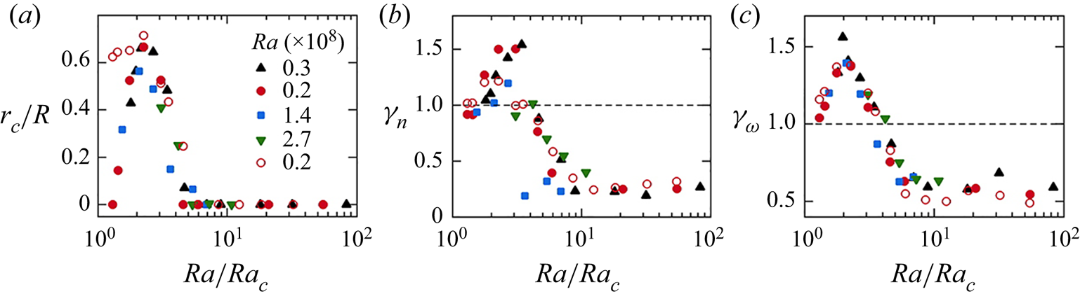
We further investigate the parameter regime in which the inverse-centrifugal motion of cyclones occurs. We define the region boundary $r_{c}$ for anomalous vortex motion as the mean radial velocity of cyclones $\langle u_r \rangle _\xi \ge 0$ for $r\le r_{c}$, and $\langle u_r \rangle _\xi <0$ for $r>r_{c}$. As shown in figure 4(c), $r_{c}$ is thus the second zero crossing of the radial profile $\langle u_r \rangle _\xi (r)$. Figure 5(a) shows $r_{c}/R$ as a function of $Ra/Ra_c$. We find $r_{c}=0$ for $Ra/Ra_c\ge 4$, and $r_{c}$ exceeds zero when $Ra/Ra_c$ decreases below 4, reaching a peak at $Ra/Ra_c\approx 2$. With further decreasing in $Ra/Ra_c$, we see that $r_{c}$ decreases, and the experimental data indicate the trend that $r_{c}$ eventually approaches zero near the onset of convection $Ra/Ra_c\approx 1$. Near onset, our numerical data show a higher value of $r_{c}$ than the experimental one, presumably owing to the insufficient numerical data evaluating the velocity profile $\langle u_r \rangle _\xi (r)$. Otherwise, results of $r_{c}/R$ for various $Ra$ collapse approximately onto one single curve. We calculate in the central region ($r\le 0.5R$) the ratios of the number density $\gamma _n$ and the vorticity magnitude $\gamma _{\omega }$ of the anticyclones over the cyclones. Figures 5(b) and 5(c) present results of $\gamma _n$ and $\gamma _{\omega }$ as functions of $Ra/Ra_c$, respectively. We see that data of $\gamma _n$ and $\gamma _{\omega }$ for various $Ra$ also exhibit similar dependence of $Ra/Ra_c$. For $Ra/Ra_c>10$, $\gamma _n$ and $\gamma _{\omega }$ are constants irrespective of $Ra/Ra_c$, while $\gamma _n$ and $\gamma _{\omega }$ increase when $Ra/Ra_c\le 10$, and have a maximum at $Ra/Ra_c\approx 2$. When $Ra/Ra_c<2$, the two ratios $\gamma _n$ and $\gamma _{\omega }$ decrease with further decreasing $Ra/Ra_c$, and approach unity at the onset of convection.

Figure 5.

(a) The region boundary $r_c/R$ for the inverse-centrifugal motion of cyclones. (b) The ratio $\gamma _n$ of the number density of anticyclones over cyclones. (c) The ratio $\gamma _{\omega }$ of vorticity amplitude of anticyclones over cyclones. Results are shown as functions of $Ra/Ra_c$. Data for $Ra=2.0\times 10^{7}$ and $\varGamma _{a}=3.8$ (circles), ${Ra=3.0\times 10^{7}}$ and $\varGamma _{a}=3.8$ (up-triangles), $Ra=1.4\times 10^{8}$ and $\varGamma _{a}=2.0$ (squares), and $Ra=2.7\times 10^{8}$ and $\varGamma _{a}=2.0$ (down-triangles). The open circles are numerical data.

The observed asymmetry of the vorticity field in the anomalous regime is attributed to the centrifugal effect. As the centrifugal force drives continuously hot (cold) fluid parcels towards (away from) the centre of the convection cell, the background fluid temperature in the central region increases and exceeds global mean fluid temperature (Hart & Olsen Reference Hart and Olsen1999; Liu & Ecke Reference Liu and Ecke2011; Horn & Aurnou Reference Horn and Aurnou2019). Thus in the central region, the temperature difference of the cold anticyclones from the background fluid becomes greater than that of the warm cyclones. Since such a temperature anomaly is proportional to the buoyancy forcing on the vortices, it is positively correlated to the vorticity magnitude of the vortices (Portegies et al. Reference Portegies, Kunnen, van Heijst and Molenaar2008; Grooms et al. Reference Grooms, Julien, Weiss and Knobloch2010). It is also believed that the fluid warming in the central region enhances the stability of the anticyclonic flows, leading to a larger population of anticyclones. As a result, we find in figures 5(b) and 5(c) that both the number density and the vorticity magnitude of the anticyclones exceed the cyclonic values.

The aforementioned vortex dynamics and symmetric properties of the vorticity field reveal four distinct flow regimes depending on the rotation rates. (I) A randomly diffusive regime in the slow rotating limit, with $Ra$ being one order in magnitude larger than $Ra_{c}$. In this flow regime, the vortices move in a random manner, yielding $\langle u_r \rangle _\xi \approx 0$, and $r_{c}/R$ is close to zero. Since at the measured fluid height the cyclones have a greater population as well as a larger vorticity magnitude than the anticyclones, $\gamma _n$ and $\gamma _{\omega }$ are both less than unity but independent of $Ra/Ra_{c}$. (II) A centrifugation-influenced regime ($4\le Ra/Ra_{c}\lesssim 10$) where the magnitude of $\langle u_r \rangle _\xi$ increases linearly with $r$ (figure 4b). We observe that warm cyclones (cold anticyclones) move radially inwards (outwards), which is in agreement with the centrifugal effect. (III) An inverse-centrifugal regime ($1.6\le Ra/Ra_{c}\le 4$) in which the cyclones exhibit anomalous outward motion in the inner region with $r\le r_{c}$ (figure 4c). In this flow regime, anticyclones become the dominant flow structures in the sense that both $\gamma _n$ and $\gamma _{\omega }$ greatly exceed unity (figures 5b,c). In the outer region ($r\ge r_{c}$), the centrifugal effect of fluid warming becomes insignificant, and we observe their inward cyclonic motion, as $\langle u_r \rangle _\xi$ for cyclones decreases with increasing $r$ and becomes negative. (IV) The asymptotic regime in the rapid rotation limit ($Ra/Ra_{c}<1.6$), where $r_{c}$ approaches zero and the opposite radial motions of cyclones and anticyclones recover (figure 4h).

6. Vortex centrifugal motion

6.1. Formation of vortex clusters

We have seen that in the inverse-centrifugal regime, the symmetry of the vorticity field is broken, with the anticyclonic vortices dominating the cyclones in both strength and population. We show below that in this regime, the vortices self-organize into clusters in which the anticyclones dominate the long-range correlated vortex motion, leading to the inverse-centrifugal motion of the cyclones.

Figure 6(a) presents an example of instantaneous spatial distribution and motion of the vortices in the inverse-centrifugal regime. We find that the adjacent vortices often move in similar directions and aggregate locally, forming vortex clusters. Here, we adopt the following two criteria to identify vortex clusters (see e.g. Chen et al. Reference Chen, Dong, Be'er, Swinney and Zhang2012):

1. (1) the distance between two neighbouring vortices is smaller than 1.5 times the mean vortex diameter;

2. (2) the angle between the velocity of two adjacent vortices is less than $\theta ^{\ast }$.

Figure 6.

(a) Spatial distribution of vortex clusters. The polygons represent the Voronoi tessellations of the vortex centres. Voronoi cells within the same vortex cluster are presented in the same colour and enclosed by thick lines. The blue (red) dots denote the centroids of anticyclonic (cyclonic) vortices, with arrows indicating their velocity direction. Experimental data in a region $r\le 0.7R$ are shown. (b) The normalized cluster length $L/H$ as a function of cluster size $N$. The dashed line represents the fitted power function $L/H=A_{c}N^{\beta _{c}}$, where $A_{c}=0.079$ and $\beta _{c}=0.81$. Data in (a,b) are for $Ra=3.0\times 10^7$ and $Ra/Ra_{c}=1.97$. (c) The exponent $\beta _{c}$ as a function of $Ra/Ra_{c}$ for various $Ra$. Open circles: $Ra=2.0\times 10^7$. Solid triangles: $Ra=3.0\times 10^7$.

Our analysis over the range $30^{\circ }\le \theta ^{\ast }\le 75^{\circ }$ confirms that the results of correlated vortex motion are not sensitive to the choice of $\theta ^{\ast }$. In the following, we discuss statistical properties using $\theta ^{\ast }=60^{\circ }$.

In figure 6(a), vortex clusters are identified using the aforementioned criteria. In this Voronoi diagram of vortex centres, each cluster is enclosed by thick lines, with Voronoi cells within the same cluster presented in the same colour. We define the cluster length $L$ as the largest distance between two vortex centres within the cluster, and compute the number of vortices $N$ with each cluster. Figure 6(b) shows $L$ as a function of $N$ for $Ra=3\times 10^{7}$ and $Ra/Ra_{c}=1.97$. We find that $L(N)$ can be well fitted by a power function $L=A_cN^{\beta _c}$. Assuming that the distance between two adjacent vortices $d_{vv}$ is independent of $N$, the power exponent $\beta _c$ then reveals the dimensional properties of clusters. When $\beta _c=0.5$, vortices in a cluster are distributed isotropically in a two-dimensional plane. When $\beta _c=1$, vortices line up to form one-dimensional clusters. Figure 6(c) shows that within the full parameter range of $Ra/Ra_{c}$ studied, $\beta _c$ increases slightly from 0.80 to 0.87 with increasing $Ra/Ra_{c}$, suggesting a fractal property of the vortex clusters: vortices in a cluster have a weak preference to be arranged along one direction, while the horizontal span of the cluster is not isotropic but dependent on the orientation.

Within each cluster, the vortices exhibit long-range correlated motions. We attribute these correlated vortex motions to the vortex–vortex interaction that occurs in a convection state where the vortices are distributed densely. Figure 7(a) shows the PDF $p(l/r_{a}$) of the distance $l$ between a downwelling vortex (anticyclone when observed in the lower half fluid layer) and its neighbouring upwelling vortices for various $Ra/Ra_{c}$. Here, $r_{a}$ is the radius of the downwelling vortex. One sees that $p(l)$ has an apparent maximum at $l_m=cr_a=1.593r_a$. Here, the constant $c$ is the ratio of the first minimum to the first zero of the zero-order Bessel function $J_0$. Since $p(l)$ represents the probability of finding upwelling vortices at a distance $l$ from a downwelling vortex, it reflects the interactions between adjacent counter-rotating vortices. Figure 7(b) shows an example of the vorticity profile $\omega (s)$ of two opposite-signed neighbouring vortices, with the coordinate $s$ measuring the distance to the centre of the downwelling vortex along the connecting line. We see that within the core region ($s< l_m$), the vorticity profile $\omega (s)$ is well described by $J_0(s)$, and $\omega (s)$ reaches a first minimum at $s=l_m$, where $p(l)$ is maximum. Such a pairwise vorticity profile is commonly observed within vortex clusters in our experiment.

Figure 7.

(a) The PDFs of the distance $l$ between an anticyclone and its neighbouring cyclones within a cluster, normalized by the radius of the anticyclone $r_{a}$. The vertical dashed line shows a maximum $p(l/{r_{a}})$ at $l=l_m=cr_{a}$. (b) Vorticity profile $\omega (s/{r_{a}})$ of an opposite-signed vortex pair along the centreline $s$. The anticyclonic radius $r_{a}$ is defined by the radial position where $\omega (s/{r_{a}})$ crosses zero. Open circles: experimental data. Solid line: the scaled zero-order Bessel functions $J_0(k_s/{r_{a}})\omega (0)/J_0(0)$, where $k=2.405$ is the first zero of $J_0$. The two vertical dashed lines indicate the centres of the anticyclone and the cyclone at $s_1=0$ and $s_2=cr_{a}$. The inset shows the vorticity distribution of this vortex pair, with the dashed line being the centreline. (c) Schematic plot of the interaction between a pair of opposite-signed convective columnar vortices at the upper layer (top) and lower layer (bottom). The blue curve represents the vorticity profile of a downwelling vortex, which creates a background vorticity field that influences the motion of an adjacent upwelling vortex (denoted by the red circle). Data are for $Ra=3.0\times 10^7$ and $Fr=0.27$.

We provide the following interpretation for the most probable vortex separation $l_m$. We consider the motion of warm, upwelling vortices in the vicinity of a cold, downwelling vortex. Observed in the lower half fluid layer ($z< H/2$), the cold vortex gives rise to a negative background vorticity gradient in the core region ($s< l_{m}$), but a positive vorticity gradient outside the vortex core ($s>l_{m}$) (see a schematic drawing in figure 7c). The theory of vortex motion on a vorticity gradient (Schecter & Dubin Reference Schecter and Dubin1999) suggests that an upwelling vortex, which possesses negative vorticity in the lower half-layer in our case, moves down the vorticity gradient due to the background shear flow. Thus inside the core region ($s< l_{m}$), the upwelling vortex moves away from the downwelling vortex centre, but moves towards it when $s>l_{m}$. Since a vortex with positive vorticity moves up a background vorticity gradient, the upwelling vortex undergoes the same translational motions in the upper half-layer. As a result, we find $s=l_{m}$ to be the most probable radial position where an upwelling vortex is located as shown in figure 7(a). For the same reason, one finds most probably a downwelling vortex at a radial distance $s=cr_c$ from an upwelling vortex centre (with $r_c$ being the radius of the upwelling vortex). Therefore, we conclude that two opposite-signed convective columnar vortices have a trend of forming a stable pair and exhibit correlated motions.

6.2. Centrifugal motion of clustered vortices

We have shown that it is the interaction between adjacent opposite-signed vortices that organizes individual vortices to form vortex clusters. Within each vortex cluster, the translational motion of the vortices is closely correlated and restricted with each other. In the following, we make comparative studies of the radial motions of clustered vortices (inside clusters) and isolated vortices (outside clusters).

Figure 8 shows the ensemble-averaged radial velocity $\langle u_r\rangle _{\xi }$ for the vortices in clusters with various sizes $N$. For isolated cyclones that move individually (i.e. $N=1$), $\langle u_r\rangle _{\xi }$ is negative and its magnitude increases approximately linearly with $r$, indicating the normal inward motion of cyclones. However, for clustered cyclones ($N\ge 2$), $\langle u_r\rangle _{\xi }$ becomes positive, which implies anomalous outward motion. We see that the slope of $\langle u_r\rangle _{\xi }(r)$ increases when $N$ increases up to 5. Therefore, clustered cyclones gain a larger velocity of inverse-centrifugal motion when the cluster size increases. The velocity profile of anticyclones exhibits a cluster size dependence similar to that of the cyclones, except that for $N=1$, $\langle u_r\rangle _{\xi }(r)$ is positive, since isolated anticyclones move outwardly.

Figure 8.

Ensemble-averaged radial velocity ${\langle u_r\rangle _{\xi }}$ of the vortices as a function of $r/R$ for various cluster sizes $N$. Data are for (a) cyclones and (b) anticyclones. Results for $Ra=2.0\times 10^7$ and $Ra/Ra_{c}=2.26$.

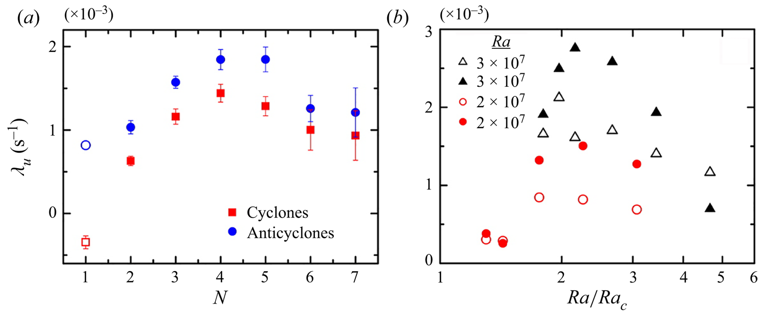
We determine the slope $\lambda _u$ of the velocity profile through fitting the data $\langle u_r\rangle _{\xi }$ in the region $0\le r\le 0.5R$ using (5.1). Results for $\lambda _u$ as a function of cluster size $N$ for $Ra/Ra_c=2.67$ are shown in figure 9(a). We see clearly that in this inverse-centrifugal regime, $\lambda _u$ for cyclones changes sign when $N$ exceeds 1. Data for both types of vortices suggest a similar trend for $N\ge 2$, i.e. $\lambda _u$ increases with $N$ for small cluster sizes and reaches a maximum at $N=5$. We also note that for small cluster size, $\lambda _u$ is considerably larger for anticyclones than for cyclones.

Figure 9.

Mobility $\lambda _u$ of vortex motion determined from the slope of ${\langle u_r\rangle _{\xi }}(r)$: (a) $\lambda _u$ as a function of $N$ for $Ra=2.0\times 10^7$ and $Ra/Ra_{c}=2.26$; (b) $\lambda _u$ as a function of $Ra/Ra_{c}$ for various $Ra$. Open symbols are data for isolated anticyclones ($N=1$). Solid symbols are data for clustered anticyclones ($N>1$).

When vortices inside a cluster move collectively, they share a similar radial velocity profile ${\langle u_r\rangle _{\xi }}(r)$. It is thus reasonable to consider all vortices inside the cluster as a single structure that undergoes radial motion driven by the centrifugal force. Here, we interpret the radial motion of vortex clusters using a Langevin-type equation analogous to (1.2) in § 1 (see also discussions in Ding et al. Reference Ding, Chong, Shi, Ding, Lu, Xia and Zhong2021). For a given initial radial position of a cluster, its radial mobility is given by $\lambda _u\approx |1/(2t_c)-\sqrt {1/(4t_c^2)+ \zeta }|$, where the relaxation time $t_{c}=M/\eta$ for the cluster's motion is given by the inertia mass $M$ of all vortices inside the cluster, $\eta$ is the dynamic viscosity, ${\zeta }=\varOmega ^{2}{\langle }{\delta }T{\rangle }$ is the coefficient of the net centrifugal force for all clustered vortices, and ${\langle }{\delta }T{\rangle }$ is the averaged temperature anomaly of the vortex cluster. Since in the inverse-centrifugal regime both the population and vorticity strength of anticyclones overrides that of cyclones, the net centrifugal force is positive, thus the vortex cluster moves outwardly.

As shown in figure 9(a), the mobility of clusters ${\lambda _u}$ is in the order of $10^{-3}$ s$^{-1}$, and $t_{c}\approx 10$ s in the inverse-centrifugal regime (see Ding et al. Reference Ding, Chong, Shi, Ding, Lu, Xia and Zhong2021); we find $1/(2t_c)\gg \lambda _u$, $\zeta {\ll }1/(2t_c)^2$, thus $\lambda _u\approx {\zeta }t_c=\varOmega ^{2}{\langle }{\delta }T{\rangle }M/\eta$. With increasing cluster size $N$, the inertia mass $M$ of the cluster increases. We suggest that it is the dominating factor for an enlarged ${\lambda _u}$ for clusters of intermediate size ($N\approx 5$). For very large cluster sizes ($N\ge 5$), we infer that viscous damping may become significant to influence cluster motion, and thereby $\lambda _u$ decreases.

Figure 9(b) presents $\lambda _u$ as a function of $Ra/Ra_{c}$ for isolated ($N=1$, open symbols) and clustered ($N>1$, solid symbols) anticyclones. Data for two sets of $Ra$ are shown for comparison. One sees that for a given $Ra$ and $Ra/Ra_{c}$, $\lambda _u$ is greater for clustered anticyclones than for isolated anticyclones. For all cases, $\lambda _u$ has a maximum at $Ra/Ra_{c}\approx 2$. We see that the maximum $\lambda _u$ for clustered anticyclones is nearly twice that of the isolated ones for both $Ra$ numbers. We also see that $\lambda _u$ increases further when a larger $Ra$ is chosen. These results demonstrate that the radial motion of anticyclones is enhanced by the collective motion to a great extent.

6.3. Froude number dependence of the vortex mobility

The mobility $\lambda _{u}$ represents the primary features of radial motion for both isolated and clustered vortices. We suggest that the non-monotonic dependence of $\lambda _{u}$ on $Ra/Ra_{c}$ shown in figure 9(b) is thus owing to the decreasing vorticity magnitude ${\vert }\omega {\vert }$ that competes with the increasing rotation rate $\varOmega$. Following discussions in § 6.2, we have $\lambda _u\approx {\zeta }t_c=\varOmega ^{2}\,{\delta }T\,m/\eta$. The temperature anomaly ${\delta }T$ of the convective vortices represents the buoyancy forcing, which is predicted to be proportional to the vorticity magnitude of the vortices (Portegies et al. Reference Portegies, Kunnen, van Heijst and Molenaar2008; Grooms et al. Reference Grooms, Julien, Weiss and Knobloch2010). Thus the mobility of clusters can approximate to $\lambda _u\approx c^*(z)\varOmega ^2\,{\vert }\omega {\vert }\,m/\eta$, with the coefficient $c^*(z)$ depending on the fluid depth. This approximate relation implies that the mobility of the vortices is determined not only by the rotating rate but also by the vorticity magnitude of the vortices.

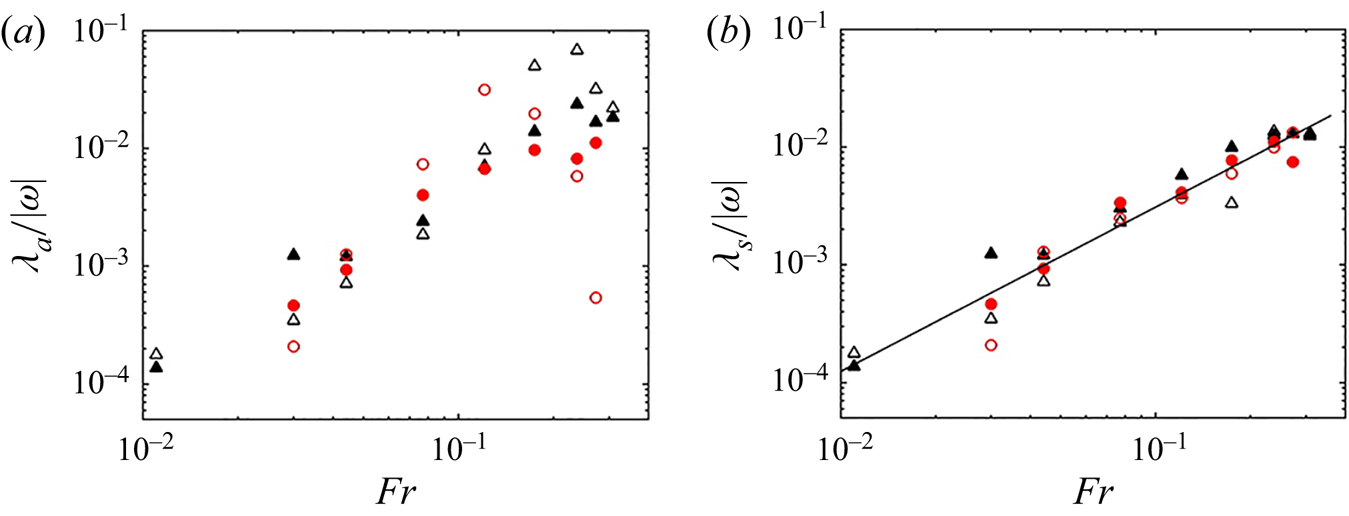
In figure 10, we show the scaled mobility $\lambda _a/{\vert }\omega {\vert }$ as a function of $Fr$ for both types of vortices. Here, $\lambda _a$ is determined by linear fitting of the radial velocity profile ${\langle u_r\rangle _{\xi }}(r)$ shown in figure 9 for both isolated ($N=1$) and clustered ($N>1$) vortices. Since $\lambda _a/{\vert }\omega {\vert }=c^{*}(z)\,\varOmega ^2m/\eta$, the scaled mobility is expected to increase when the rotation rate increases. Our experimental results in figure 9(a) show that this is the case, as $\lambda _a/{\vert }\omega {\vert }$ for both cyclones and anticyclones grows rapidly with increasing $Fr$ in the full parameter range studied. Meanwhile, we see that results for $\lambda _a/{\vert }\omega {\vert }$ are scattered, and there exists a notable difference between the cyclonic and anticyclonic data for given $Fr$ and $Ra$.

Figure 10.

(a) The mobility $\lambda _{a}/|\omega |$ of all vortices scaled by the vorticity magnitude as a function of $Fr$.(b) The scaled mobility $\lambda _{s}/|\omega |$ of isolated vortices as a function of $Fr$. Results are for $Ra=2.0\times 10^7$ (red circles) and $Ra=3.0\times 10^7$ (black triangles). Open symbols: cyclones. Solid symbols: anticyclones. The solid line represents a power-function fit with exponent $1.40\pm 0.13$.

We suggest that the vortex interaction of vortices forming clusters may disturb individual vortex motion and modify the vortex mobility. In support of this argument, we determine the mobility $\lambda _{s}$ for isolated vortices, calculating the slope of the velocity profile ${\langle u_r\rangle _{\xi }}(r)$ (e.g. shown in figure 9) for both cyclones and anticyclones for the case of $N=1$. Results for $\lambda _s/{\vert }\omega {\vert }$ are shown as a function of $Fr$ in figure 10(b). We see that the discrepancy of $\lambda _s/{\vert }\omega {\vert }$ between isolated cyclones and anticyclones is minor. Moreover, data for $\lambda _s/{\vert }\omega {\vert }$ for various $Ra$ collapse onto a power-law function $\lambda _s/{\vert }\omega {\vert }\propto Fr^{1.40\pm 0.13}$ in the full parameter range of $Fr$ studied, suggesting a general scaling relationship. These results imply that the mobility of isolated vortices scaled by the magnitude of their vorticity can be determined adequately by the Froude number.

7. Vortex lifespan

Observations of the evolution of vortex structures suggest that the generation and disappearance of the vortices occur seemingly randomly in time. In this section, we present the statistical analysis of the lifespan of vortices. We calculate the number $N(t)$ of vortices that have a lifespan longer than time $t$. Figure 11 shows the results for $N(t)/N_0$ as a function of time for various $Ra/Ra_c$. Here, $N_0$ is the number of all vortices observed over the course of the experiment. We see that for both types of vortices, $N(t)/N_0$ decreases exponentially in large time limits. The solid lines in figure 11 represent the fitted exponential functions to the data, that is, $N(t)/N_0=A\exp (-t/{\tau })$, with $\tau$ being the characteristic lifespan of the vortices, and $A$ a fitting coefficient. The exponential decay law of $N(t)$ in figure 11 can be understood considering that each vortex has a constant disappearing probability $p$ in unit time. The decreasing rate is expected to be proportional to the number of existent vortices, i.e. ${\rm d}N/{\rm d}t=-pN$. This simple model leads to the exponential decay law for $N(t)$, and yields the characteristic vortex lifespan $\tau =1/p$ of the long-lived vortices.

Figure 11.

Results of $N(t)/N_0$ as a function of time for (a) cyclones and (b) anticyclones, for $Ra=3.0\times 10^7$. The solid curves represent the fitted exponential function $N(t)/N_0=A\exp (-t/{\tau })$.

Meanwhile, we notice that in a short time ($t\ll {\tau }$), $N(t)$ decays faster than the fitted exponential curves, as shown in figure 11, suggesting that short-lifespan vortices may die out with a higher probability. It could be that a subset of these vortices arises from vortex interactions or background turbulence, and exhibits distinct behaviour of evolution compared to the long-lived, coherent vortices. Nevertheless, these short-lifespan vortices have little influence on the statistical properties of the vortex lifespan $\tau$.

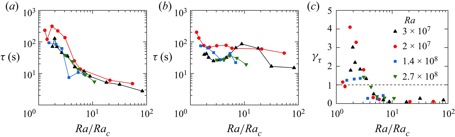
The characteristic lifespan $\tau$ for both types of vortices at different $Ra/Ra_c$ is shown in figure 12. For a given $Ra$, the lifespan of anticyclones shows a clear increasing trend with decreasing $Ra/Ra_c$ (figure 12a). The lifespan of cyclones, however, exhibits a non-monotonic dependence on $Ra/Ra_c$. Figure 12(b) shows that a local minimum of $\tau$ appears within the inverse-centrifugal regime $1.6\le Ra/Ra_c\le 4$, which is attributed to the fact that cyclones undergo the normal inward motion in the outer region ($r>r_c$), but are forced to move outwardly in the inner region ($r< r_c$) owing to the vortex clustering effect (see figure 5c). The convergent radial motion of the cyclones results in a relatively short lifespan $\tau$ on average, maintaining a constant vortex number density as observed in the experiment.

Figure 12.

The characteristic lifespan ${\tau }$ of (a) anticyclones and (b) cyclones, as a function of $Ra/Ra_c$. (c) The ratio $\gamma _\tau$ of the lifespan of anticyclones to that of cyclones, as a function of $Ra/Ra_c$.

To compare the lifespan of the two types of vortices, we show in figure 12(c), as a function of $Ra/Ra_c$, the ratio $\gamma _{\tau }$ of the lifespan of anticyclones over the cyclones. We see that the lifespan of anticyclones is around one order of magnitude shorter than that of cyclones in the flow regime (I) (when $Ra/Ra_c\ge 10$). As $Ra/Ra_c$ decreases below 10, $\gamma _{\tau }$ increases. When the system enters into the inverse-centrifugal regime (III) ($Ra/Ra_c\le 4$), the lifespan of anticyclones starts to override that of cyclones. The remarkable similarity in the $Ra/Ra_c$ dependence of $\gamma _{\tau }$, $\gamma _n$ and $\gamma _\omega$ (see figures 5b,c) suggests that the vortex lifespan is strongly influenced by the centrifugal effects.

We examine the radial dependence of the vortex lifespan in flow regimes where the radial motion of vortices is prominent. Here, we calculate the number $N_{r0}(t)$ of vortices that arise at an initial radial position $r_0\pm 0.05R$ and have a lifespan larger than $t$. Figures 13(a) and 13(b) show $N_{r0}/N_0$ as a function of time for cyclones and anticyclones, respectively, for various $r_0$, with $N_0$ being a normalization coefficient. Here, $N_{r0}/N_0$ appears to depend sensitively on the initial radial position $r_0$, and for each $r_0$, $N_{r0}/N_0$ follows persistently the exponential decay in time. In figures 13(c) and 13(d), we show results of the lifespan $\tau$ as a function of $r_0$ for two types of vortices. It is notable that $\tau$ depends sensitively on the initial location for $Ra/Ra_c=2.67$, while in the centrifugation-influenced regime ($Ra/Ra_c=4.66$), $\tau$ appears relatively constant with varying $r_0$. In the inverse-centrifugal regime ($Ra/Ra_c=2.67$), the lifespan of cyclones decreases with increasing $r_0$ in the inner region ($r\lesssim r_c$), reaching a minimum at the region boundary ($r_0\approx r_c$), followed by an increase in the outer region ($r\gtrsim r_c$). Hence cyclones around the boundary of the inverse-centrifugal region have the shortest lifespan. For anticyclones, $\tau$ decreases monotonically with $r_0$. These results also reveal that vortices generated within the inner region ($r_0< r_c$) possess in general a longer lifespan than vortices generated in the outer region. We suggest two reasons that may be responsible for vortices in the inner region having longer lifespans. First, since vortex clusters form mostly in the inner region (see figure 6a), they have larger inertia and are more stable against perturbations from the background turbulent flows, which stabilizes the structure of the vortices within. Second, annihilation and merging events of adjacent vortices occur less frequently within clusters as the clustered vortices are moving in a collective manner.

Figure 13.

Results for $N_{r0}/N_0$ as a function of time for (a) cyclones and (b) anticyclones arising at various initial radial positions. Data are for $Ra/Ra_c=2.67$, $Ra=3\times 10^7$. The characteristic lifespan $\tau$ of (c) cyclones and (d) anticyclones as a function of $r_0/R$ for two sets of $Ra/Ra_c$. Solid symbols: $Ra/Ra_c=2.67$. Open symbols: $Ra/Ra_c=4.66$. The vertical dashed lines denote the inverse-centrifugal region boundary $r_0=r_c$ for $Ra/Ra_c=2.67$.

8. Summary and discussions

A major emphasis of previous studies in rotating convection has been on the flow structures of the convective vortices in rotating RBC (Vorobieff & Ecke Reference Vorobieff and Ecke2002; Sprague et al. Reference Sprague, Julien, Knobloch and Werne2006; Portegies et al. Reference Portegies, Kunnen, van Heijst and Molenaar2008; Grooms et al. Reference Grooms, Julien, Weiss and Knobloch2010; Nieves et al. Reference Nieves, Rubio and Julien2014; Rajaei et al. Reference Rajaei, Kunnen and Clercx2017; Shi et al. Reference Shi, Lu, Ding and Zhong2020) and partly on their stochastic translational motions (Sakai Reference Sakai1997; King & Aurnou Reference King and Aurnou2012; Noto et al. Reference Noto, Tasaka, Yanagisawa and Murai2019; Chong et al. Reference Chong, Shi, Ding, Ding, Lu, Zhong and Xia2020; Ding et al. Reference Ding, Chong, Shi, Ding, Lu, Xia and Zhong2021). We investigate here their spatial distribution, lifespan and radial motion in the parameter ranges $2.0\times 10^7\le Ra\le 2.7\times 10^8$, $1.7\times 10^{-5}\le Ek\le 2.7\times 10^{-4}$ and $1.2\times 10^{-3}\le Fr\le 0.31$, which cover four flow regimes of vortex motion: (I) random vortex diffusion, (II) centrifugal-forced radial motion, (III) inverse-centrifugal motion, and (IV) asymptotic centrifugal motion. We report that under slow rotations with $Ra\gtrsim 10\,Ra_{c}$, the vortices undergo Brownian-type random motion, i.e. the mean square displacement (MSD) of the vortices increases first in time as $t^2$ in the ballistic regime, and then linearly in the diffusive regime. Our close inspection of the PDFs of the vortex displacements reveals that, however, the ballistic motion of the vortices is non-Gaussian at small time intervals. Furthermore, we show that in the limit of slow rotations ($Ra\approx 80\,Ra_{c}$), the vortices are randomly distributed over the horizontal plane, with the PDFs of the Voronoi cell areas of the vortices well described by the standard $\varGamma$ distribution.

With modest strength of rotations, the centrifugal force influences the dynamics of the vortices. We observed that in this flow regime with $4\,Ra_{c}\le Ra\le 10\,Ra_{c}$, cyclones move radially towards the rotation axis, while anticyclones migrate outwards. Thus the MSD of the vortices increases faster than a linear function of time at a large time. Moreover, we note that the ensemble average of the radial velocity $\langle u_r\rangle _\xi$ of cyclones (anticyclones) is negative (positive) and decreases (increases) linearly with respect to $r$. The centrifugal motion of the vortices in a background of turbulent fluctuation can be interpreted through an extended Langevin model incorporating centrifugal acceleration. In this flow regime, we find that the horizontal scale of the vortices, and thus the mean area $A$ of vortex Voronoi cells, decreases with increasing rotating rate. The size distribution of the Voronoi cells deviates from the standard $\varGamma$ distribution, as reflected by the decreasing of their standard deviation $\sigma (A/{\langle }A{\rangle })$.

Under rapid rotations with $1.6\,Ra_{c}\le Ra\le 4\,Ra_{c}$, the mean area of the Voronoi cells of the vortices decreases significantly, signifying that the vortices are distributed densely. In this convection state, the hydrodynamic interaction of neighbouring vortices becomes prominent to influence the vortex dynamics. We report the existence of a most probable separation between two adjacent counter-rotating vortices that tend to form a vortex pair and move collectively. Such vortex interactions eventually lead to the formation of large-scale vortex clusters. As a result, the size of the vortex Voronoi cells becomes diversified, thus $\sigma (A/{\langle }A{\rangle })$ increases with decreasing $Ra/Ra_{c}$. In this flow regime, the cold anticyclones override the warm cyclones in vorticity strength, population and lifespan, a flow field asymmetry brought about by the centrifugal effect. Within vortex clusters, the motion of the weak cyclones thus submits to that of strong anticyclones and moves outwardly in a collective manner. Within each vortex cluster, the translational motion of the vortices is long-range correlated. We show that such correlated motion of the clustered vortices exerts essential influences on their dynamics. With increasing cluster size $N$, the radial velocity $\langle u_r\rangle _{\xi } (r)$ for clustered cyclones and anticyclones increases faster with $r$, thus both types of vortices gain a larger translation velocity moving outwardly. Despite the complicated $Fr$ dependence of the scale vortex mobility $\lambda _a/{\vert }\omega {\vert }$ for all vortices, we discover in the full parameter range of $Fr$ a simple power-law scaling $\lambda _s/{\vert }\omega {\vert }\propto Fr^{1.4}$ for isolated vortices for various $Ra$ and vortex types.

Finally, an intriguing aspect of rotating convection systems is the lifespan $\tau$ of the coherent vortices. We report that the number of vortices $N(t)$ with a lifespan exceeding $t$ decays exponentially in time. Such an exponential decay law suggests that the convective vortices experience a constant rate $1/\tau$ of disappearance (e.g. through merging or annihilation events). The fact that spatial- and time-averaged vortex number density $n$ remains constant implies that the convective vortices are generated with constant rate $1/\tau$. Our studies of the statistical properties of the vortex lifespan may provide valuable insights into the evaluation of the vortex distributions and dynamics in rotating convection.

We have shown in this work the rich and intriguing vortex dynamics in rotating RBC. There remain numerous issues requiring further investigations. Prominent among those is the origin of the Brownian but non-Gaussian diffusion of the vortex displacements. Such non-Gaussian diffusive motion becomes apparent at short time scales. Another crucial issue awaiting theoretical descriptions is the hydrodynamic interactions among closely located convective vortices that give rise to the long-range collective motion of the vortices. What are the implications of the vortex dynamics presented in this study for the correlated vortex motion observed in giant gaseous planets and other large-scale geophysical and astrophysical flows (Li et al. Reference Li, Ingersoll, Klipfel and Brettle2020; Gavriel & Kaspi Reference Gavriel and Kaspi2021, Reference Gavriel and Kaspi2022; Mura et al. Reference Mura2021)? We expect future progress in answering these questions.