2 RMHD description of a forming current sheet

We study an incompressible plasma with a strong and uniform $z$ -directed guide magnetic field, such that the behaviour of the $x$ – $y$ plane flow and magnetic field can be modelled by the resistive RMHD equations (Kadomtsev & Pogutse Reference Kadomtsev and Pogutse1973; Strauss Reference Strauss1976; Schekochihin et al. Reference Schekochihin, Cowley, Dorland, Hammett, Howes, Quataert and Tatsuno2009). These read, in cgs units,

and

Here, $\unicode[STIX]{x1D719}$ is the streamfunction of the plasma fluid velocity in the $x$ – $y$ plane, $\boldsymbol{u}$ , such that $\boldsymbol{u}=(-\unicode[STIX]{x2202}_{y}\unicode[STIX]{x1D719},\unicode[STIX]{x2202}_{x}\unicode[STIX]{x1D719})$ and $\unicode[STIX]{x1D713}$ is the flux function of the in-plane magnetic field $\boldsymbol{B}$ , so that $\boldsymbol{B}=(-\unicode[STIX]{x2202}_{y}\unicode[STIX]{x1D713},\unicode[STIX]{x2202}_{x}\unicode[STIX]{x1D713})$ (in addition, an asymptotically strong magnetic field in the $\hat{z}$ direction is assumed to be present). The Poisson bracket of two fields $P,Q$ is $\{P,Q\}=\unicode[STIX]{x2202}_{x}P\unicode[STIX]{x2202}_{y}Q-\unicode[STIX]{x2202}_{y}P\unicode[STIX]{x2202}_{x}Q$ ; the plasma mass density is $\unicode[STIX]{x1D70C}_{0}$ .

We normalize the RMHD equations according to $\unicode[STIX]{x1D713}\rightarrow \unicode[STIX]{x1D713}/\sqrt{4\unicode[STIX]{x03C0}\unicode[STIX]{x1D70C}_{0}}$ , $\unicode[STIX]{x1D719}\rightarrow \unicode[STIX]{x1D719}$ , $t\rightarrow t$ , $x\rightarrow x$ , $y\rightarrow y$ and $\unicode[STIX]{x1D702}\rightarrow \unicode[STIX]{x1D702}$ . This non-standard normalization does not include any characteristic length scales or magnetic field strengths to avoid confusion due to changes in these quantities as the current sheet evolves. With these normalizations, the RMHD equations lose their explicit mass density dependence to read:

and

Figure 1.

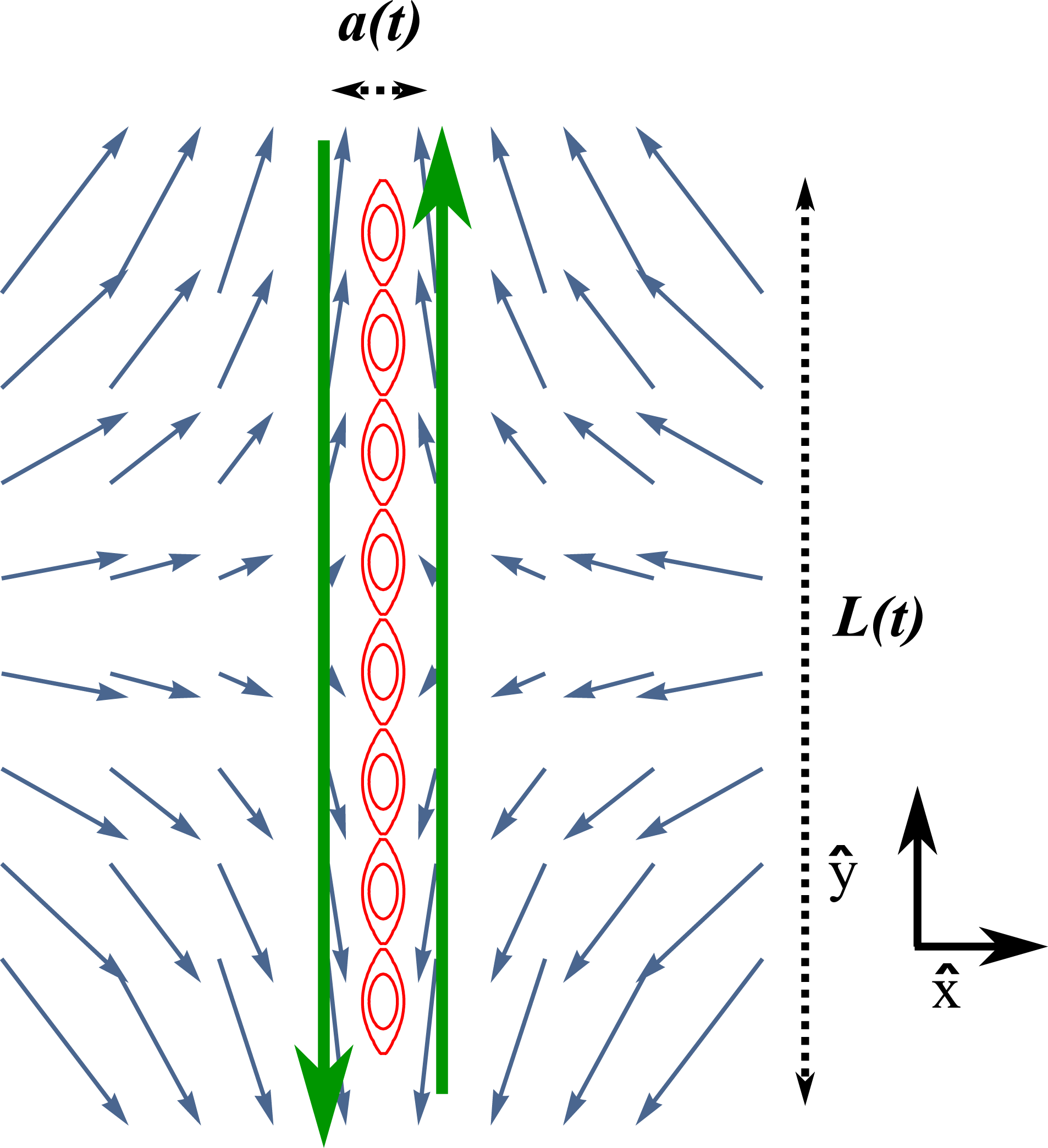
Schematic configuration of forming current sheet, which is characterized by a width $a(t)$ and a length $L(t)$ . Thick green lines represent the equilibrium magnetic field, the blue vector field the flow and the red magnetic island chain the tearing perturbation.

We will employ these equations to study an ideal MHD current sheet that forms as a result of plasma flows. This serves as the equilibrium for the paper’s tearing stability analysis. The sheet is depicted schematically in figure 1. While many specific mathematical descriptions of such a sheet may exist, a clear, analytic tearing stability analysis makes desirable two characteristics: first, that the sheet’s magnetic field have no $y$ dependence, in order to allow Fourier analysis in this direction; second, that the sheet’s flow pattern be simple enough to allow for the use of coordinate transformations and sheared wave vectors in the tearing calculation. A model that meets these goals is an extension of the one-dimensional Chapman–Kendall (Chapman & Kendall Reference Chapman and Kendall1963) sheet:

where the current sheet width $a(t)$ narrows with time according to

with $a_{0}$ being the initial ( $t=0$ ) width and $\unicode[STIX]{x1D6E4}_{0}(t)$ a time-dependent shear parameter. The magnetic field given by this flux function is

with

the characteristic time-dependent strength of the sheet’s magnetic field. The corresponding streamfunction is given by

In our study of the ideal MHD behaviour (§ 4), our analysis is limited to the specific case of constant $\unicode[STIX]{x1D6E4}_{0}(t)=\unicode[STIX]{x1D6E4}_{0}$ , while in our study of linear and nonlinear tearing (§§ 5 and 6), our analysis applies for slowly varying $\unicode[STIX]{x1D6E4}_{0}(t)$ as well. Functions (2.5) and (2.9) together obey (2.3) and (2.4) in the ideal limit $\unicode[STIX]{x1D702}=0$ for any magnetic field shape $f$ . The streamfunction $\unicode[STIX]{x1D719}_{0}(x,y,t)$ is the same used in the Chapman–Kendall model and represents a general expansion of flow about a stagnation point. For functions $f$ yielding magnetic fields which are locally linear about $x=0$ , the first term in the expansion of (2.5) is the Chapman–Kendall flux function, $\unicode[STIX]{x1D713}_{0}(x,t)=B_{0y}a_{0}x^{2}/[2a(t)^{2}]$ . At times, our calculation will require a specific form for the magnetic field; in these cases, we will often take the $f$ that yields a Harris sheet (Harris Reference Harris1962), such that

and

We have constrained the equilibrium magnetic field to only have a component in the ${\hat{y}}$ direction, the magnitude of which is independent of $y$ , to enable Fourier analysis in $y$ . Thus, the length of our current sheet is not mathematically defined by the expressions given so far. However, the current sheet is stretched by a flow along its length, $u_{y}=\unicode[STIX]{x1D6E4}_{0}(t)y$ , which grows with distance along the sheet $y$ in the same sense that the flow into the sheet, which causes current sheet compression, $u_{x}=-\unicode[STIX]{x1D6E4}_{0}(t)x$ , decreases with decreasing $x$ . We may thus define an effective length

which grows as the width of the current sheet shrinks. This definition leaves the product $a(t)L(t)$ constant, consistent with incompressibility. Another way to think about this length is to consider placing two markers in the current sheet that move with the flow. If the markers are initially separated in $y$ by a distance $L_{0}$ , their future separation is given by (2.12). This exponential behaviour of the current sheet width and length agrees with trends seen in simulations (Sulem et al. Reference Sulem, Frisch, Pouquet and Meneguzzi1985; Friedel, Grauer & Marliani Reference Friedel, Grauer and Marliani1997; Biskamp Reference Biskamp2005).

Thus, current sheet formation in this scenario proceeds through a combination of thinning ( $a$ decreasing in time, as given by (2.6)), stretching ( $L$ increasing with time, as given by (2.12)) and magnetic field strengthening ( $B_{y}$ increasing with time, given by (2.8)). The exponential growth in the magnetic field strength is consistent with the exponential growth and collapse of the spatial scales. All $x$ -scales and separations decrease in time exponentially; this includes the $x$ -separation between two given magnetic fields lines frozen into the fluid, and this is the reason the magnetic field strength is increasing.

3 Fourier analysis of a forming current sheet

The aim of this paper is to study the behaviour of a small perturbation to the forming current sheet described by (2.5) and (2.9), such that $\unicode[STIX]{x1D713}(x,y,t)=\unicode[STIX]{x1D713}_{0}(x,t)+\unicode[STIX]{x1D6FF}\unicode[STIX]{x1D713}(x,y,t)$ and $\unicode[STIX]{x1D719}(x,y,t)=\unicode[STIX]{x1D719}_{0}(x,y,t)+\unicode[STIX]{x1D6FF}\unicode[STIX]{x1D719}(x,y,t)$ . Evaluating (2.3) and (2.4) for the behaviour of the perturbation in linear order yields

and

We Fourier analyse these perturbations along the ${\hat{y}}$ direction, such that $\unicode[STIX]{x1D6FF}\unicode[STIX]{x1D719}=\unicode[STIX]{x1D719}_{1}(x,t)\exp [\text{i}k(t)y]$ and $\unicode[STIX]{x1D6FF}\unicode[STIX]{x1D713}=\unicode[STIX]{x1D713}_{1}(x,t)\exp [\text{i}k(t)y]$ . Because the current sheet is evolving, we take a wave vector $k(t)$ that also evolves. The postulate for $k(t)$ is guided by the intuition that the number of islands $N$ characterizing a given mode should remain constant as the current sheet stretches, such that

This postulate also allows the cancellation of the explicit $y$ -dependence in terms containing $\unicode[STIX]{x2202}_{x}\unicode[STIX]{x1D719}_{0}$ in (3.1) and (3.2). With this choice, a critical simplification in enabling the analysis that follows, (3.1) and (3.2) using (2.9) reduce to

and

Sections 4 and 5 are concerned with solving these equations.

4 Effect of flow on perturbations in ideal MHD

The main aim of this paper is to analyse the resistive tearing dynamics of a current sheet as it forms due to flow. Before considering this topic, however, it is worthwhile examining the ideal behaviour of small perturbations that occur in a forming current sheet. These are changes due to the effect of the flow alone and not due to resistive tearing, which remain when $\unicode[STIX]{x1D702}$ is set to zero in (3.5). This behaviour describes the system when the gradients in the forming current sheet are not yet sufficient to drive a tearing instability whose growth rate overwhelms the flow shear rate, so any tearing that may occur is a small perturbation to the dominant flow-driven behaviour. Our focus is on tearing-like modes: those that are even with respect to the midplane $x=0$ and that are associated with non-zero perturbed flux at $x=0$ . We find that these perturbations are compressed and stretched by the flow. However, we also note in passing a way in which this analysis may be adapted to treat other types of modes.

The ideal MHD behaviour of our current sheet may be studied by setting $\unicode[STIX]{x1D702}=0$ in (3.5). In addition, in this section, we consider the special case of constant flow rate,

We now perform a transformation of coordinates in (3.4) and (3.5) such that

which moves the system to coordinates which are compressed with the flow. The transformation gives

and

Solving (4.4) for $\unicode[STIX]{x1D719}_{1}$ and substituting into (4.3) then yields a differential equation for $\unicode[STIX]{x1D713}_{1}$ . For each mode $k_{0}$ , there will come a time at which $\text{e}^{2\unicode[STIX]{x1D6E4}_{0}t^{\prime }}\unicode[STIX]{x2202}_{x^{\prime }}^{2}\gg \text{e}^{-2\unicode[STIX]{x1D6E4}_{0}t^{\prime }}k_{0}^{2}$ . After this time, which we discuss at the end of this section, the terms proportional to $k_{0}^{2}$ may be dropped from (4.3). When this is possible, the differential equation for $\unicode[STIX]{x1D713}_{1}$ may be Fourier analysed in time $t^{\prime }$ , such that $\unicode[STIX]{x1D713}_{1}=\unicode[STIX]{x1D6F9}_{1}(x^{\prime })\text{e}^{-\text{i}\unicode[STIX]{x1D714}t^{\prime }}$ . This gives the following equation relating $\unicode[STIX]{x1D714}$ and the derivatives of $\unicode[STIX]{x1D6F9}_{1}$ , where we have plugged in (2.5) for the equilibrium flux function:

The solutions to this differential equation will depend on the specific form of $f$ . However, the equation alone shows the general effect of flow on perturbations that exist in the current sheet. Equation (4.5) demonstrates that under the transformation (4.2), the behaviour of the perturbations appears identical to perturbations in a flow-free system (consider setting $\unicode[STIX]{x1D6E4}_{0}\rightarrow 0$ in (4.5)) except for the redefinition

where $\unicode[STIX]{x1D714}$ is the frequency of the perturbation in the current sheet evolving due to flow and $\unicode[STIX]{x1D714}_{0}$ is the corresponding frequency in a static magnetic configuration. Thus, for every mode that exists in a static magnetic configuration ((2.5) with $\unicode[STIX]{x1D6E4}_{0}=0$ ) of frequency $\unicode[STIX]{x1D714}_{0}$ , we can find a corresponding mode in the evolving current sheet. The mode in the developing current sheet has the same structural form as the static mode, but is expressed as a function of the transformed coordinates and has a modified frequency $\unicode[STIX]{x1D714}$ . This modified frequency is found by solving (4.6) for $\unicode[STIX]{x1D714}$ as a function of the corresponding $\unicode[STIX]{x1D714}_{0}$ and $\unicode[STIX]{x1D6E4}_{0}$ , so that

which reduces, as expected, to $\unicode[STIX]{x1D714}=\unicode[STIX]{x1D714}_{0}$ in the case of no flow.Footnote ¹

We would like to consider tearing-like modes, for which $\unicode[STIX]{x1D6F9}_{1}(0)\neq 0$ . These modes are more straightforward than other modes which may exist in the sheet. Consider evaluating (4.4) at $x^{\prime }=0$ . Since the magnetic field passes through 0, and hence $\unicode[STIX]{x2202}_{x^{\prime }}\unicode[STIX]{x1D713}_{0}|_{x^{\prime }=0}=0$ , this evaluation immediately reveals that $\unicode[STIX]{x2202}_{t^{\prime }}\unicode[STIX]{x1D713}_{1}|_{x^{\prime }=0}=0$ . In ideal MHD, magnetic flux is conserved, and since the centre of the sheet has no equilibrium velocity or magnetic field, the value of the flux there must be constant. Separating the perturbation according to $\unicode[STIX]{x1D713}_{1}=\unicode[STIX]{x1D6F9}_{1}(x^{\prime })\text{e}^{-\text{i}\unicode[STIX]{x1D714}t^{\prime }}$ then gives two possibilities: either $\unicode[STIX]{x1D6F9}_{1}(0)=0$ or $\unicode[STIX]{x1D714}=0$ . While in general modes in the sheet may obey either condition, tearing-like modes must have $\unicode[STIX]{x1D6F9}_{1}(0)\neq 0$ and hence $\unicode[STIX]{x1D714}=0$ . Thus, for these modes, (4.5) reduces to:

This equation, stated in the primed coordinates, is unmodified from its flow-free equivalent, so we see that the effect of the flow on these modes is simply to compress them as represented by the primed coordinates. (The sheared wave vector taken in the Fourier analysis of § 3 will also stretch the islands.) Note that it also follows from (4.4) and $\unicode[STIX]{x1D714}=0$ that $\unicode[STIX]{x1D719}_{1}=0$ ; there is no flow, perturbed or equilibrium, in the primed coordinates.

Figure 2.

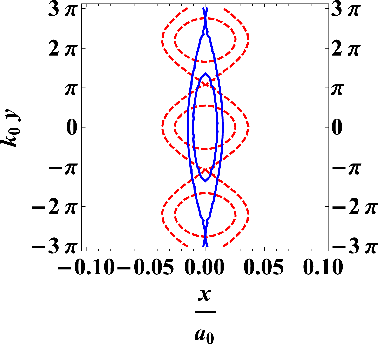
Contour lines of $\unicode[STIX]{x1D713}_{0}+\unicode[STIX]{x1D713}_{1}$ for a tearing-like mode undergoing ideal evolution. The perturbed flux, $\unicode[STIX]{x1D713}_{1}$ , is given by (4.9), while $\unicode[STIX]{x1D713}_{0}$ is given by $\unicode[STIX]{x1D713}_{0}=-B_{0y}a_{0}\cos ([\unicode[STIX]{x03C0}/2][x/a(t)])$ , $a(t)=a_{0}\text{e}^{-\unicode[STIX]{x1D6E4}_{0}t}$ . The configuration is shown for $\unicode[STIX]{x1D6E4}_{0}t=0.1$ (dashed red line) and $\unicode[STIX]{x1D6E4}_{0}t=1$ (solid blue line). The strength of the perturbation relative to the equilibrium magnetic fields is given by $\unicode[STIX]{x1D713}_{1}(0)/B_{0y}=0.001$ . The islands are compressed in $x$ and lengthened in $y$ by the flow, just as the sheet width and wave vector are; indeed, if the islands were instead plotted in terms of $k(t)y$ and $\boldsymbol{x}/a(t)$ , the islands would appear to be constant.

As an example, we can select the flux function with $f[x/a(t)]=-\text{cos}([\unicode[STIX]{x03C0}/2][x/a(t)])$ , which gives the magnetic field $\boldsymbol{B}={\hat{y}}B_{0y}\text{e}^{\unicode[STIX]{x1D6E4}_{0}t}\unicode[STIX]{x03C0}\sin ([\unicode[STIX]{x03C0}/2][x/a(t)])/2$ , which is locally linear about $x=0$ . This configuration allows a simple solution (unlike the Harris equilibrium (2.10)). We solve (4.8) for $\unicode[STIX]{x1D6F9}_{1}$ , constraining our solution to be even in $x^{\prime }$ . Stating the perturbed flux function in terms of the unprimed coordinates then gives

with $\unicode[STIX]{x1D713}_{1}(0)$ a constant. We see here the expected self-similar compression; the mode will also be stretched by the sheared wave vector. This behaviour is illustrated in figure 2.

The analysis in this section is only valid once $\text{e}^{2\unicode[STIX]{x1D6E4}_{0}t^{\prime }}\unicode[STIX]{x2202}_{x^{\prime }}^{2}\gg \text{e}^{-2\unicode[STIX]{x1D6E4}_{0}t^{\prime }}k_{0}^{2}$ . Taking a typical value $\unicode[STIX]{x2202}_{x^{\prime }}^{2}\sim 1/a_{0}^{2}$ (as is true in (4.9)), we see that this condition is just that $k(t)a(t)\ll 1$ ; in other words, for this analysis to be valid, the mode’s wavelength $\unicode[STIX]{x1D706}(t)=2\unicode[STIX]{x03C0}/k(t)$ must be much longer than the sheet thickness at the same time, $a(t)$ . Since a mode’s wavelength grows with time while the sheet thickness shrinks with time, this condition will become better satisfied for any mode as time increases. On the other hand, as time increases, the resistive term in (3.5) will also become more important, and the sheet’s tendency to tear will increase. Our ideal analysis will only be useful for modes for which the condition $k(t)a(t)\ll 1$ is satisfied before resistivity becomes important. We can estimate that resistivity becomes important at the time $t_{\text{cr}}$ when the flow-free tearing rate of the fastest growing mode becomes equal to the flow shear rate $\unicode[STIX]{x1D6E4}_{0}$ . The growth rate of the fastest-growing mode can be found by balancing the expressions in (1.1) and (1.2), which have opposite scaling with $k$ , to give $\unicode[STIX]{x1D6FE}_{0,\text{max}}=\unicode[STIX]{x1D702}^{1/2}B_{y}^{1/2}/a^{3/2}$ . This rate becomes equal to $\unicode[STIX]{x1D6E4}_{0}$ when $t=t_{\text{cr}}=\log [(\unicode[STIX]{x1D6E4}_{0}a_{0}^{3/2})/(\unicode[STIX]{x1D702}^{1/2}B_{0y}^{1/2})]/(2\unicode[STIX]{x1D6E4}_{0})$ . Meanwhile, $k(t)a(t)=1$ when $t=\log (k_{0}^{2}a_{0}^{2})/(4\unicode[STIX]{x1D6E4}_{0})$ . Thus, wave vectors for which the ideal analysis is valid at least for some period of time (that is, for which the $k_{0}^{2}$ terms may be dropped prior to resistivity becoming important) are given by $k_{0}a_{0}\ll (\unicode[STIX]{x1D6E4}_{0}a_{0}/B_{0y})(B_{0y}a_{0}/\unicode[STIX]{x1D702})^{1/2}\equiv k_{0,\text{ideal}}a_{0}$ , which for high Lundquist number plasmas is a weak limitation.Footnote ² Nonetheless, the analysis does not answer the question of what happens for modes with $k_{0}a_{0}\gg (\unicode[STIX]{x1D6E4}_{0}a_{0}/B_{0y})(B_{0y}a_{0}/\unicode[STIX]{x1D702})^{1/2}$ or what happens to modes of shorter wavelength before $\text{e}^{2\unicode[STIX]{x1D6E4}_{0}t^{\prime }}\unicode[STIX]{x2202}_{x^{\prime }}^{2}\gg \text{e}^{-2\unicode[STIX]{x1D6E4}_{0}t^{\prime }}k_{0}^{2}$ . For these cases, we rely on the intuition that the flow should still stretch and compress tearing-type modes, since it does not present an instability source (see below). However, the form of this stretching and compressing, and the resulting deformation of the tearing mode magnetic islands, will be more complicated than the simple picture in this section.

No modes in the sheet, including those for which the analysis is not valid, will be Kelvin–Helmholtz unstable, for two reasons. First, the specific flow pattern that we choose, equation (2.9), lacks the inflection points necessary for Kelvin–Helmholtz instability; second, even if we were to relax our flow model to include patterns with inflection points, for flows that remain sub-Alfvénic with respect to (2.8), no instability would exist (Loureiro et al. Reference Loureiro, Schekochihin and Uzdensky2013).

However, the flow will affect perturbations, and the aim of this section has been to describe this effect, showing that they are reshaped ideally by the flow. This is the dominant behaviour of any perturbations in the sheet before narrowing $a(t)$ and sharpening gradients lead to significant tearing. This tearing stage is treated next.

5 Linear tearing instability

As the width of the current sheet decreases, the importance of the resistive term in the induction equation increases until appreciable reconnection begins to occur. After this time, reconnection will proceed in a manner modified by flow, first traversing the linear stage of the tearing mode. Previous studies of the effect of flow on the linear tearing mode studied static configurations (Bulanov et al. Reference Bulanov, Syrovatskii and Sakai1978; Paris & Sy Reference Paris and Sy1983; Biskamp Reference Biskamp1986; Chen & Morrison Reference Chen and Morrison1990; Bulanov Reference Bulanov2016). In these cases, the flow alters the separable exponential growth of the tearing mode; that is, $\unicode[STIX]{x1D713}_{1}$ may be written as

where $\unicode[STIX]{x1D6FE}_{0}$ is the tearing growth rate without flow, and $h$ is some function of flow strength $\unicode[STIX]{x1D6E4}_{0}$ which either increases or decreases mode growth rate.

We argue, however, that this formulation is not a proper way of describing the effect of flows that cause change in the equilibrium configuration. Such flows introduce time dependence into (3.4) and (3.5), such that the perturbation cannot immediately be separated into $x$ -dependent and $t$ -dependent parts. Applying the coordinate transformation (4.2), as we did when considering ideal MHD behaviour, does not resolve this problem, since the transformation leads the resistive term in (3.5) to develop explicit time dependence, even in the case of constant $\unicode[STIX]{x1D6E4}_{0}$ . Instead, exponential time dependence must be separated out using a multiple scale formulation. The application of this approach reveals that flows add slow time dependence to the standard eigenfunction $\unicode[STIX]{x1D6F9}_{1}(x)$ ; however, they do not alter the separable exponential growth.

Let us study the effect of flow on the linear tearing rate by formulating the system in terms of two time scales, one (shorter) which governs the growth of the perturbation and another (longer) which governs the evolution of the current sheet (Bender & Orszag Reference Bender and Orszag2013). When the first of these time scales is much shorter than the second, the ratio of the two scales can be used as a small parameter in which to expand $\unicode[STIX]{x1D713}_{1}$ and $\unicode[STIX]{x1D719}_{1}$ . The time in current sheet development when this approach is valid, and its relationship to the overall reconnection of the current sheet, are discussed in § 7. We again assume for simplicity $\unicode[STIX]{x1D6E4}_{0}(t)=\text{constant}$ , though the analysis that follows may in principle be generalized to any relatively slowly evolving $\unicode[STIX]{x1D6E4}_{0}(t)$ for which $\unicode[STIX]{x2202}_{t}\unicode[STIX]{x1D6E4}_{0}(t)/\unicode[STIX]{x1D6E4}_{0}\lesssim \unicode[STIX]{x1D6E4}_{0}(t)$ . Let us define:

and

with $\unicode[STIX]{x1D6FE}_{0}$ a value representing the characteristic strength of the tearing growth, which could for instance be the flow-free linear tearing mode growth rate calculated with the values of $k$ , $a$ and $B_{y}$ instantaneously assumed by the mode and the forming current sheet. These time scales are related by the small parameter

This quantity will decrease with time as the current sheet narrows and the tendency to tear increases while the flow strength remains constant. Quantities influenced only by the flow, $k(t)$ and $\unicode[STIX]{x1D713}_{0}(x,t)$ , vary on the slow time scale $\unicode[STIX]{x1D70F}$ , while the perturbation varies on the fast time scale $\hat{t}$ . This separation was not possible in the ideal stage, when the time scale of the perturbation was comparable to the overall sheet evolution time scale.

In terms of these new time scales, (3.4) and (3.5) read

and

Writing these equations in terms of $\unicode[STIX]{x1D70F}$ and $\unicode[STIX]{x1D716}$ yields

and

We can then write our solution as an expansion in $\unicode[STIX]{x1D716}$ , so that

and equivalently for $\unicode[STIX]{x1D713}_{1}(x,\unicode[STIX]{x1D70F})$ . This expansion separates the fast tearing mode growth from the slow evolution of the perturbations, which is in general a non-separable function of space and time. Note that here $\hat{\unicode[STIX]{x1D6FE}}(s)$ represents $\mathit{O}(1)$ corrections to the growth rate $\unicode[STIX]{x1D6FE}_{0}$ , such that the full growth rate in units of $t$ instead of $\hat{t}$ reads $\unicode[STIX]{x1D6FE}(\unicode[STIX]{x1D70F})=\unicode[STIX]{x1D6FE}_{0}\hat{\unicode[STIX]{x1D6FE}}(\unicode[STIX]{x1D70F})$ .

These expansions may be plugged in to (5.7) and (5.8) to yield equations governing the perturbation at each order in $\unicode[STIX]{x1D716}$ . The $O(\unicode[STIX]{x1D716}^{0})$ equations read:

and

These equations are identical to the classic flow-free tearing mode eigenvalue equations (Furth et al. Reference Furth, Killeen and Rosenbluth1963), but with time-dependent coefficients, growth rates $\unicode[STIX]{x1D6FE}(\unicode[STIX]{x1D70F})=\unicode[STIX]{x1D6FE}_{0}\hat{\unicode[STIX]{x1D6FE}}(\unicode[STIX]{x1D70F})$ and eigenfunctions $\unicode[STIX]{x1D6F9}_{1,0}(x,\unicode[STIX]{x1D70F})$ . Therefore, the growth rates and eigenfunctions have the same form as their flow-free equivalents, but with $k$ , $B_{y}$ and $a$ modified to be time dependent. Corrections to the growth rate which are explicitly proportional to $\unicode[STIX]{x1D6E4}_{0}$ do not appear because terms in the equations governing the perturbation which are explicitly proportional to $\unicode[STIX]{x1D6E4}_{0}$ are of the same order as the time dependence of $k$ and $\unicode[STIX]{x2202}_{x}\unicode[STIX]{x1D713}_{0}$ (which prevents the equations from being completely separable). The tearing growth rate, which is the separable part of the perturbation growth, does not depend explicitly on $\unicode[STIX]{x1D6E4}_{0}$ , in contrast to tearing growth rates in sheets with flow that does not alter the equilibrium.

Therefore, the strongest effect of flows causing current sheet formation on the tearing mode is just to add time dependence to the tearing mode growth rates and eigenfunctions (Furth et al. Reference Furth, Killeen and Rosenbluth1963; Coppi et al. Reference Coppi, Galvão, Pellat, Rosenbluth and Rutherford1976), such that to zeroth order in $\unicode[STIX]{x1D716}$

and equivalently for $\unicode[STIX]{x1D713}_{1}$ , where the growth rate can be replaced by the classical expressions

or

depending on whether the mode in question is an FKR mode, a Coppi mode or the fastest-growing mode, found by balancing the Coppi and FKR expressions. The eigenfunctions read

with $\unicode[STIX]{x1D6F9}_{1}$ and $\unicode[STIX]{x1D6F7}_{1}$ the normal flow-free tearing eigenfunctions, which depend on $k$ and $a$ . While the flow will not affect the separable exponential growth of the perturbation, it will alter how the perturbation changes in time in a non-separable way through its addition of time dependence to the eigenfunctions. The strength of this correction is given by straightforward differentiation of (5.16):

and

both of which will be proportional to $\unicode[STIX]{x1D6E4}_{0}$ because $\unicode[STIX]{x2202}_{t}k$ and $\unicode[STIX]{x2202}_{t}a$ are.

As an example, we can evaluate this effect for the magnetic perturbation in the Harris sheet (2.10). Recall that the magnetic eigenfunction in the flow-free case is given by

with the boundary condition that the eigenfunction go to zero at $x=\pm \infty$ (Furth et al. Reference Furth, Killeen and Rosenbluth1963). For (2.10), the appropriate eigenfunction is

From here, we can evaluate that

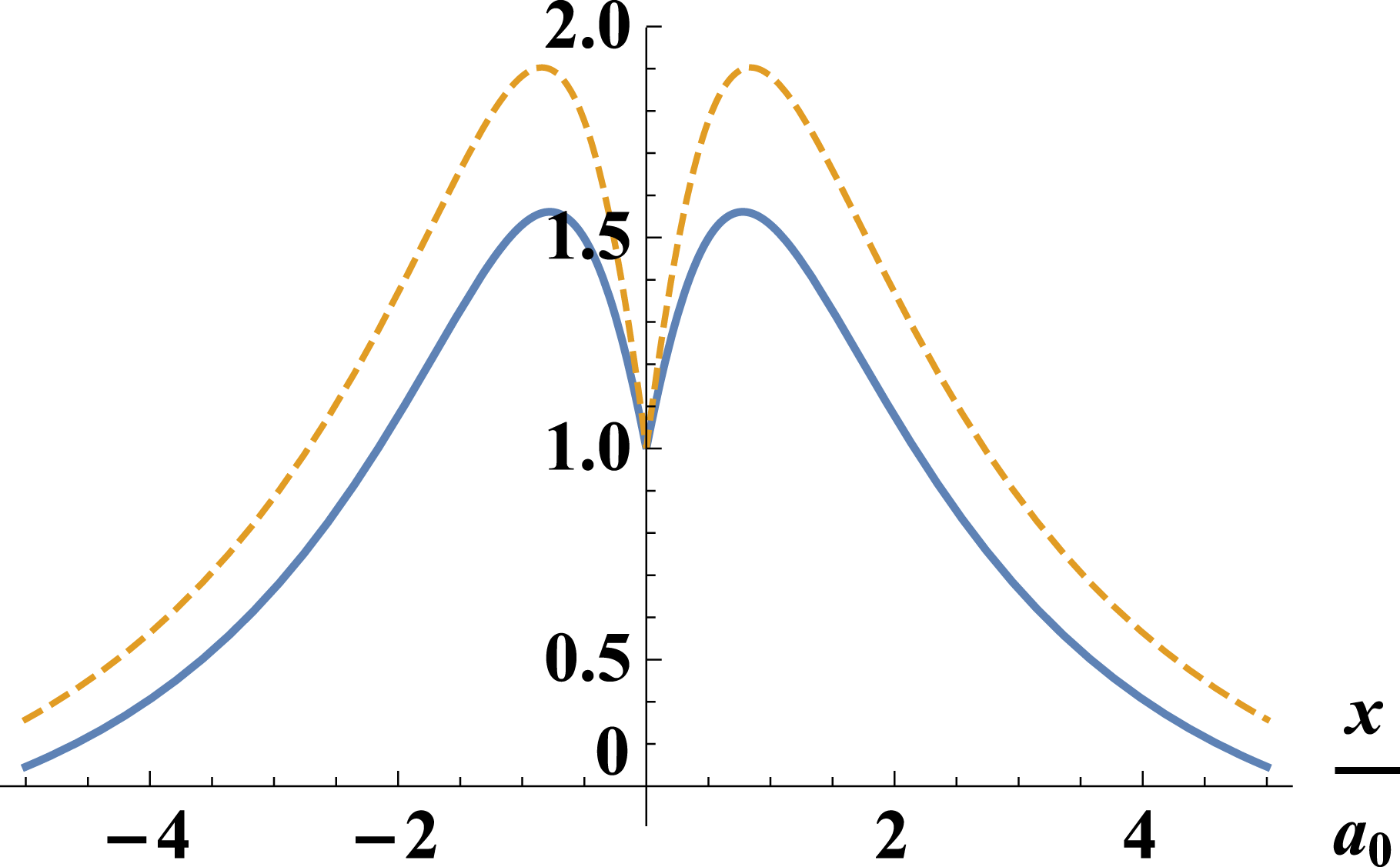
where we have substituted (3.3) and (2.6). This is a strictly positive quantity, representing a tendency of flow to enhance mode growth. An example eigenfunction evolution is shown in figure 3, which shows that the eigenfunction tends to grow as time increases. Note that this growth is clearly non-separable; for example, the eigenfunctions value does not change at $x=0$ while it does change elsewhere. Thus, this effect cannot be expressed as a correction to the separable exponential growth rate, as in (5.1).

Figure 3.

Evolution of $\unicode[STIX]{x1D6F9}_{1,0}(x,t)$ for the Harris sheet eigenfunction (5.20), for $k(t)$ and $a(t)$ given by (2.6) and (3.3) with $\unicode[STIX]{x1D6E4}_{0}(t)=\text{constant}$ , for $k_{0}a_{0}=0.5$ . The solid blue line is evaluated at $t=0$ , while the orange dotted line is evaluated at $\unicode[STIX]{x1D6E4}_{0}t=0.1$ .

The reader may also be interested in the nature of higher-order corrections of the flow given by the equations at $O(\unicode[STIX]{x1D716})$ . At this order, we have

and

Since $\unicode[STIX]{x1D6F9}_{1,0}$ , $\unicode[STIX]{x1D6F7}_{1,0}$ and $\unicode[STIX]{x1D6FE}(\unicode[STIX]{x1D70F})$ are found from the $O(\unicode[STIX]{x1D716}^{0})$ equations, these expressions are coupled differential equations in $x$ only for $\unicode[STIX]{x1D6F9}_{1,1}$ and $\unicode[STIX]{x1D6F7}_{1,1}$ which may be solved to find small, non-separable corrections to the tearing mode eigenfunctions. Note that even these perturbations grow exponentially with the tearing growth rates given by (5.13), (5.14) and (5.15), as appropriate.

Thus, we have shown that in a developing current sheet in the regime where $\unicode[STIX]{x1D6FE}\gg \unicode[STIX]{x1D6E4}_{0}$ , flows affect the separable exponential tearing growth only implicitly, by making $a$ , $B_{y}$ , and $k$ time-dependent, and not through a correction that explicitly depends on flow of the type represented in (5.1). The flows will add slow, non-separable time dependence to the tearing mode eigenfunctions, and we have stated the lowest-order strength of this effect in (5.17) and (5.18); additional corrections could in principle be calculated from (5.22) and (5.23). But this slow time dependence is overwhelmed by the strong, exponential tearing mode growth rate.

6 Nonlinear theory

As the linear stage develops, it will eventually reach a point where the width of the forming magnetic island is comparable to the width of the inner resistive layer and the linear approximation is no longer valid. A Coppi mode will at this point enter Waelbroeck X-point collapse (which will not be affected by the flow because it proceeds at a rate comparable to that of the fastest tearing mode, much faster than the flow rate (Waelbroeck Reference Waelbroeck1993; Loureiro et al. Reference Loureiro, Cowley, Dorland, Haines and Schekochihin2005)). An FKR mode will enter the Rutherford phase (Rutherford Reference Rutherford1973), which we examine here.

We adapt the original flow-free Rutherford theory to the evolving system using the coordinate transformation (4.2) and look for the growth of the tearing mode island width  $W$ . This process reveals two effects that modify the flow-free theory in the evolving case. First, adding time dependence to $k$ and $a$ leads to an increase in the island width’s Rutherford growth rate through time. However, proper inclusion of the changing background and flow-dependent terms also yields a narrowing of the island width due to the compression of the equilibrium. This effect does not change the functional dependence of the growth but reduces it slightly by a constant scalar factor.

In the Rutherford phase, nonlinear instability behaviour is analysed through Ohm’s law (3.5). In flow-free analysis, the terms $-B_{0y}\text{i}k\unicode[STIX]{x1D719}_{1}$ and $-\unicode[STIX]{x1D702}k^{2}\unicode[STIX]{x1D713}_{1}$ are considered negligible in (3.5); the addition of flow will not change this, and so we can state the perturbation’s governing equation as

Taking the case of constant $\unicode[STIX]{x1D6E4}_{0}$ (similar results hold for slowly varying $\unicode[STIX]{x1D6E4}_{0}$ and the techniques in this section may be adapted for non-slowly varying $\unicode[STIX]{x1D6E4}_{0}$ as well) and transforming coordinates in this equation according to (4.2) yields

In this coordinate system, the perturbation growth is caused by a resistivity that appears to grow with time. This apparent growth is due to the sharpening of gradients, caused by the compressing flow. We thus apply the flow-free procedure (Rutherford Reference Rutherford1973; Biskamp Reference Biskamp2005) in these coordinates, adapting it to deal with the time dependence.

To do this, we will need to determine the behaviour of island width $W$ and tearing mode stability index $\unicode[STIX]{x1D6E5}^{\prime }$ in both the unprimed and primed systems. Recall the expression for the tearing mode island width in the unprimed system:

Note that since $\unicode[STIX]{x2202}_{x}^{2}\unicode[STIX]{x1D713}_{0}$ increases with time, the island width of a perturbation with constant $\unicode[STIX]{x1D713}_{1}$ decreases with time. In the primed frame, the island width $W^{\prime }$ is defined in terms of the constant-in-time $\unicode[STIX]{x2202}_{x^{\prime }}\unicode[STIX]{x1D713}_{0}$ , so that

which we could also see by considering that lengths in the unprimed frame are related to lengths in the primed frame by $x^{\prime }=x\text{e}^{\unicode[STIX]{x1D6E4}_{0}t}$ . For the tearing mode stability index $\unicode[STIX]{x1D6E5}^{\prime }$ , recall the definition (Furth et al. Reference Furth, Killeen and Rosenbluth1963) $\unicode[STIX]{x1D6E5}^{\prime }\equiv \lim _{\unicode[STIX]{x1D716}\rightarrow 0}\left[\unicode[STIX]{x2202}_{x}\unicode[STIX]{x1D713}_{1}(\unicode[STIX]{x1D716})-\unicode[STIX]{x2202}_{x}\unicode[STIX]{x1D713}_{1}(-\unicode[STIX]{x1D716})\right]/\unicode[STIX]{x1D713}_{1}$ . Since this quantity is an inverse length, it transforms according to

For the Harris sheet (2.10) for $k(t)a(t)\ll 1$ , we can then evaluate

Returning to equation (6.2), we can rewrite the second derivative of the flux function in terms of $W^{\prime }$ and $(\unicode[STIX]{x1D6E5}^{\prime })^{\prime }$ , so that

Relating $W^{\prime }$ to $\unicode[STIX]{x1D713}_{1}$ using (6.4) (noting that $\unicode[STIX]{x2202}_{x^{\prime }}^{2}\unicode[STIX]{x1D713}_{0}$ is time independent) then gives

Using (6.4) to also state our result in terms of island width in the unprimed system yields

where we have stated our result in terms of $\unicode[STIX]{x1D6E5}^{\prime }(t)\sim 1/[k(t)a(t)^{2}]\sim \text{e}^{3\unicode[STIX]{x1D6E4}_{0}t}/(k_{0}a_{0}^{2})$ .

This reveals a significant acceleration in the growth of the island width due to the change with time of the tearing mode stability index. This effect was used in the treatment of the nonlinear phase in Uzdensky & Loureiro (Reference Uzdensky and Loureiro2016) through its inclusion of time dependence on $L$ (or equivalently $N/k$ ) and $a$ in nonlinear growth rates. However, the treatment in Uzdensky & Loureiro (Reference Uzdensky and Loureiro2016) did not consider that the apparent width of the island is also decreased due to the flow and the changing equilibrium, which is reflected in our subtraction of $\unicode[STIX]{x1D6E4}_{0}W$ . To further understand the effect of this term, we can first integrate (6.9) to find

with $W_{0}$ the island width at the start of the nonlinear phase, here defined as $t=0$ . The equivalent integration for (6.9) without the subtracted $\unicode[STIX]{x1D6E4}_{0}W$ term gives

For large times, the behaviour of both (6.10) and (6.11) is dominated by their final terms, which differ only by a factor of $3/4$ . The functional behaviour of the nonlinear stage is thus the same in the evolving case, and using the flow-free equations with time dependence added, as done in Uzdensky & Loureiro (Reference Uzdensky and Loureiro2016), will only overestimate the growth by a scalar factor of order unity.

7 Conclusion: effect of flow in the context of current sheet development

We have presented a self-consistent RMHD model for a current sheet forming due to flow and examined the development of the tearing instability in it. Here, we review our analysis. A current sheet configuration will begin its evolution in a state where its characteristic width $a$ is such that the gradients in the current sheet are not sufficient to cause strong tearing. In this regime, the behaviour of any pre-existing magnetic islands in the sheet can be studied using ideal MHD. This study, conducted in § 4, shows that the islands will be compressed in $x$ and stretched in $y$ , with their aspect ratio increasing, by the flow.

As the current sheet compresses, it will become more unstable to tearing perturbations. Tearing behaviour becomes important approximately at the time $t\sim t_{\text{cr}}$ when the magnitudes of the rates controlling current sheet evolution and tearing are comparable, i.e. $\unicode[STIX]{x1D6E4}_{0}(t_{\text{cr}})=\unicode[STIX]{x1D6FE}_{0,\text{max}}(t_{\text{cr}})$ (Uzdensky & Loureiro Reference Uzdensky and Loureiro2016). After this time, the multiple scale formulation of § 5 will become progressively better justified as the continually narrowing current sheet causes the drive for the tearing instability to overwhelm the flow rate. In this regime, the tearing mode may be approximately described by the flow-free growth rates and eigenfunctions, with time dependence trivially added to $k$ , $B_{y}$ , and $a$ . Small corrections to the eigenfunctions may be computed, but even these will grow with the flow-free tearing mode growth rate.

Neither of these two approaches is valid during the period of time immediately surrounding $t_{\text{cr}}$ , when $\unicode[STIX]{x1D6E4}_{0}$ and $\unicode[STIX]{x1D6FE}_{0,\text{max}}$ are of roughly the same magnitude, so we cannot make any definitive conclusions about the effects of flows during this time.Footnote ³ However, we can estimate the error that this uncertainty introduces. Namely, during this period the islands grow with a tearing growth rate $\unicode[STIX]{x1D6FE}_{0,\text{max}}(t)\sim \unicode[STIX]{x1D6E4}_{0}(t_{\text{cr}})$ . But the current sheet equilibrium, and hence the tearing growth rate, whatever its form, evolve on the time scale $\unicode[STIX]{x1D6E4}_{0}^{-1}$ . Thus, the duration $\unicode[STIX]{x0394}t$ of the interval during which the two rates themselves are comparable is also of order $\unicode[STIX]{x1D6E4}_{0}^{-1}$ . The factor by which the islands grow during this interval, given by

can then be estimated as $e$ to a power of order unity. This is a finite factor, independent of resistivity, which will not have a drastic effect on island development, and thus the ideal and linear treatments together cover the most significant periods of island growth.

At the end of the linear stage, when the width of the magnetic islands exceeds that of the inner resistive layer, the mode will enter the nonlinear regime, described in § 6. Here, a simple coordinate transformation shows that to get a growth rate in the evolving sheet, one must both add time dependence to $k$ and $a$ in the flow-free expressions and subtract a term due to the strengthening of the background magnetic field. This will slightly slow the nonlinear growth relative to expressions studied in Uzdensky & Loureiro (Reference Uzdensky and Loureiro2016).

Overall, this paper provides a detailed framework for understanding how the tearing mode behaves in an evolving current sheet. While this analysis identifies some subtle effects not considered in Uzdensky & Loureiro (Reference Uzdensky and Loureiro2016), like the subtracted term in the nonlinear stage and the small corrections to the linear eigenfunctions, all in all it strengthens confidence in the use of tearing mode scalings developed in a stationary configuration to study the tearing mode in an evolving sheet, and thus in the results of several recent studies of forming current sheets (Pucci & Velli Reference Pucci and Velli2014; Comisso et al. Reference Comisso, Lingam, Huang and Bhattacharjee2016, Reference Comisso, Lingam, Huang and Bhattacharjee2017; Uzdensky & Loureiro Reference Uzdensky and Loureiro2016; Huang et al. Reference Huang, Comisso and Bhattacharjee2017).

Future work based on this paper might consider two particular areas. First, our results are strictly limited to plasmas in which uniform resistivity RMHD is valid. This excludes collisionless, and semi-collisionless, plasmas; that is, plasmas for which the resistive layer width of the current sheet is smaller than the ion skin depth $d_{i}\equiv c/\unicode[STIX]{x1D714}_{pi}$ , with $\unicode[STIX]{x1D714}_{pi}$ the ion plasma frequency, or the ion sound gyroradius $\unicode[STIX]{x1D70C}_{s}\equiv \sqrt{\left(T_{i}+T_{e}\right)m_{i}}/\left(q_{i}B_{T}\right)$ , where $T_{i}$ and $T_{e}$ are the ion and electron temperatures, respectively, $m_{i}$ is the ion mass, $q_{i}$ is the ion charge and $B_{T}$ is the total magnetic field (including the guide field in the $\hat{z}$ direction). For the fastest-growing linear mode in the sheet, found at the intersection of the FKR and Coppi regimes (Furth et al. Reference Furth, Killeen and Rosenbluth1963; Coppi et al. Reference Coppi, Galvão, Pellat, Rosenbluth and Rutherford1976), the condition on the validity of our RMHD treatment may be stated in terms of Lundquist number:

Extending our work to collisionless, or semi-collisionless, regimes where (7.2) does not hold would require a distinct analysis from that in this paper, though certain techniques that we use could likely be adapted. Such an extension is important given the weak collisionality of many plasmas in which reconnection occurs, including the magnetosphere (Ji & Daughton Reference Ji and Daughton2011).

Second, we have restricted the analysis in this paper to current sheets with straight magnetic fields due to the challenges present in formulating a two-dimensional current sheet model and in Fourier analysing perturbations in a two-dimensional equilibrium. Since we study a forming current sheet where reconnection is just beginning, $\hat{x}$ magnetic components resulting from reconnected field do not yet exist. However, it is possible that the background magnetic field from which the sheet forms is curved; indeed this is the case in the Earth’s magnetotail (Petrukovich et al. Reference Petrukovich, Artemyev, Vasko, Nakamura and Zelenyi2015), and in astrophysical situations where current sheet formation occurs because of field-line opening due to differential rotation (see, e.g. Uzdensky (Reference Uzdensky2004) and references therein). An extension of our work could consider such curved fields, perhaps by employing computational methods.

Finally, combining these two areas by studying current sheets with curved magnetic fields in collisionless plasmas is also of significant interest, as previous work has found that inclusion of two dimensional effects leads to new behaviour in collisionless reconnection (Lembege & Pellat Reference Lembege and Pellat1982; Sitnov & Swisdak Reference Sitnov and Swisdak2011).