


1. Introduction
In nonlife insurance, claims from various business lines frequently exhibit strong interdependencies. For instance, workplace accidents can generate simultaneous claims for medical expenses and lost wages, while natural disasters can simultaneously damage homes, vehicles, and businesses. These catastrophic events often exhibit spatial correlation, meaning that a disaster impacting one location tends to affect numerous structures concurrently. More broadly, systemic risks can trigger simultaneous claims across multiple insurance lines, impacting both the frequency and severity of losses.
This interconnectedness of risks is also observed in computer network failures and infectious disease outbreaks, as demonstrated during the COVID-19 pandemic. In these domains, extreme events are often interdependent. For example, widespread quarantines led to a surge in remote work, increasing network congestion and vulnerabilities that cyberattacks could exploit. This interplay of risks is crucial for nonlife insurers, as it directly influences pricing, reserving, solvency, and capital allocation strategies. Understanding the dependence between different underwriting lines is crucial for insurers’ pricing strategies, capital allocation, and risk management, particularly under solvency regulations and risk-based capital requirements.
For modeling insurance claims, the compound Poisson process is a widely accepted and standard technique. To capture dependencies in a multivariate setting, a common shock representation is often employed, see, e.g., Lindskog and McNeil (Reference Lindskog and McNeil2003). Dependence in claim severity can be modeled separately by applying a distributional copula to the joint magnitudes of the concurrent losses, conditional on a simultaneous event. This two-level approach (common shocks for frequency, copulas for severity) allows for a detailed specification of the joint dependence structure at both stages of the claim generating process. Because both components are defined at the level of individual claim events rather than aggregate losses over a fixed reporting period, the model is consistent across different time horizons: the joint distribution of cumulative losses over any interval is determined by the same set of parameters without requiring separate calibration for each time scale.
Unfortunately, the common shock model becomes increasingly parameter intensive as the number of dimensions increases. For example, the case of four business lines may require the specification of up to fifteen independent Poisson arrival processes (due to jumps that can be common to two, three, or four classes), several multivariate distributional copulas, and twenty-four jump size distributions.
An alternative approach is to apply a distributional copula directly to the aggregate claims of each class at a chosen time horizon, creating a multivariate distribution of aggregate claim amounts, see, e.g., McNeil et al. (Reference McNeil, Frey and Embrechts2005). Similarly, a distributional copula may be applied to the aggregate number of claims over a chosen time horizon, see, e.g., Bäuerle and Grübel (Reference Bäuerle and Grübel2005). This model is then reduced to modeling dependence between random variables for a given time horizon. This approach possesses several benefits, including relative parsimony in model specification and facilitating a “bottom-up” approach to multivariate modeling, whereby models are built by combining the information of marginals (lines of business) with that of the dependence structure across classes.
A significant limitation of using distributional copulas for aggregate claims is their time-horizon dependency. The copula fitted for one time period cannot be reliably extrapolated to another. Additionally, this approach necessitates ample aggregate claim data for each business class within the selected time frame. For instance, with only one year of data, fitting a copula for a one-year horizon yields only a single data point, leading to inefficient use of available information, especially when detailed individual claim data exists.
Multivariate Lévy copulas serve as a bridge between the common shock and distributional copula approaches. They specify dependence at the level of the Lévy measure through the marginal tail integrals of individual compound Poisson processes. This is the central distinction between Lévy copulas and distributional copulas applied to aggregate claims: a distributional copula describes the joint distribution of claims for a fixed horizon. The fitted copula is specific to that horizon and cannot be extrapolated to a different period without refitting. In contrast, with Lévy copulas, the joint distribution of aggregate losses over any horizon [0, t] is then automatically determined for all t via the Lévy–Khintchine formula. This yields a model that is consistent across reporting periods: the joint distribution of cumulative losses over any interval is governed by the same dependence parameter without re-estimation because the Lévy–Khintchine formula propagates the Lévy measure structure to all horizons automatically. Once individual claims data become available, all records contribute to estimation regardless of the reporting period chosen, in contrast to a distributional copula fitted to annual aggregates, which uses only one data point per year. It is worth emphasizing that data limitations for extreme events remain a challenge in both frameworks and that estimating a Lévy copula requires individual claim records rather than aggregated statistics, which may not always be available in practice.
Lévy-copulas were introduced by Kallsen and Tankov (Reference Kallsen and Tankov2006), see also Cont and Tankov (Reference Cont and Tankov2003), who laid the groundwork for subsequent studies by numerous researchers who have further explored and expanded the applications of Lévy-copulas in various fields.
Incorporating these copulas into a dynamic optimization framework, we study the problem of optimal premium setting for an insurer underwriting multiple lines of business. The insurer is modeled as a monopolistic price setter that can influence demand – and consequently, its risk exposure – through pricing decisions. Demand functions describe how policyholders respond to changes in premiums, while adverse selection is incorporated by allowing claim arrival rates to depend on premium levels.
Our approach builds upon the dynamic model of Christensen et al. (Reference Christensen, Parra-Alvarez and Serrano2021) in which a risk-averse insurer controls the premium rate vector to maximize the expected discounted lifetime utility of intermediate consumption. The present study integrates Lévy copulas, demand functions, and dynamic programming to derive optimal premium strategies that maximize the insurer’s long-run expected utility of consumption by the owner manager, under the assumption of constant absolute risk aversion (CARA) with utility function
 $U(x)=-\frac{1}{\eta}e^{-\eta x}$
and risk-aversion coefficient
 $\eta\gt 0$
.
We employ an infinite-horizon formulation primarily because of its tractability. The associated Hamilton–Jacobi–Bellman (HJB) equation reduces to an ordinary integro-differential equation whose solution does not depend on the time variable, yielding stationary optimal policies that do not vary with the remaining planning horizon. The infinite-horizon setting can be interpreted as an approximation to a long planning horizon, or as the limit of a sequence of finite-horizon problems as the time horizon grows. The same analysis can in principle be carried out over a finite horizon. However, the infinite-horizon formulation allows us to abstract from institutional constraints (annual accounting, solvency reporting cycles, etc.) in order to isolate the effect of multivariate claim dependence on optimal premium setting, which is the central focus of the paper.
In the model, the premium vector affects the wealth process through two interacting channels. On the revenue side, higher premiums increase the unit price but reduce demand, so the net effect on total revenue is ambiguous and depends on demand elasticity. On the cost side, lower demand reduces the effective claim exposure. The insurer therefore faces a trade-off between risk exposure and revenue generation, which is captured by the profile Hamiltonian Q(p) in Equation (7) once the CARA structure reduces the dynamic problem to a static optimization. The resulting optimization problem resembles that of a multiproduct monopolist with a nonseparable cost function, where costs are influenced by the dependence structure of claims.
Lévy copulas have been applied to insurance, operational risk, and finance problems: Bregman and Klüppelberg (Reference Bregman and Klüppelberg2005) and Böcker and Klüppelberg (Reference Böcker and Klüppelberg2010) used a Clayton Lévy copula for multivariate operational risk, Bäuerle and Blatter (Reference Bäuerle and Blatter2011) studied the optimal investment and reinsurance problems for a multiline insurer, and Avanzi et al. (Reference Avanzi, Cassar and Wong2011) discussed and illustrated the fitting of Lévy copulas to data. Demand-based pricing in insurance has been studied by Taylor (Reference Taylor1986) and Thomas (Reference Thomas2008) using exponential demand functions and by Hao et al. (Reference Hao, Macdonald, Tapadar and Thomas2016); Hao et al. (Reference Hao, Macdonald, Tapadar and Thomas2018); Hao et al. (Reference Hao, Macdonald, Tapadar and Thomas2019) using iso-elastic demand functions.
Asmussen et al. (Reference Asmussen, Christensen and Taksar2013) and Thøgersen (Reference Thøgersen2016) study demand functions that depend on premium and deductible for heterogeneous customers. They also obtain isoelastic demand functions in the case of partial information. Christensen et al. (Reference Christensen, Parra-Alvarez and Serrano2021) considered a dynamic model in which a risk-averse insurer controls the premium rate and deductible, under the assumption that customers differ in riskiness, and with demand functions and claim arrival rates incorporating adverse selection, which results in a combined negative effect on the aggregate arrival rate. Recently, Gudmundarson et al. (Reference Gudmundarson, Guerra and Moura2023) studied the effects of dependencies between risks in a population of prospective insurance customers on the exposure for an insurance company, depending on the company’s market share. They characterized optimal loadings and obtained an upper bound for the difference between the ruin probability and its estimate based on the company’s portfolio marginal distributions.
This study contributes to the literature on insurance pricing by integrating Lévy copula dependence structures into a dynamic, demand-based premium optimization framework. For the case of two business lines, we establish conditions under which higher dependence increases risk exposure and adversely impacts profitability using supermodular ordering. Our findings offer both theoretical insights and practical guidelines for insurers seeking to balance profitability with risk exposure in a multiline underwriting environment.
The organization of this paper is as follows. In Section 2, we present some preliminaries on multivariate insurance risk modeling, in Section 3, we introduce the dynamic premium control model and optimization problem, in Section 4, we formulate the associated Hamilton-Jacobi-Bellman equation and prove the main optimality result. In Section 5, we present a numerical example. Finally, in Section 6, we prove a result on the sensitivity of the optimal value with respect to the dependence structure. We close out the paper with a few conclusions about our work. The paper has four appendices. Appendix A reviews the theory of tail integrals and Lévy copulas, including Sklar’s theorem for Lévy processes and its specialization to compound Poisson processes. Appendix B collects the auxiliary comparison results based on supermodular ordering used in Section 6. Appendix C presents the decomposition of bivariate compound Poisson processes and the alternative single-counting-process representation underlying the three-term splitting of the Lévy cost integral in Section 5. Appendix D provides the key computational building blocks of the numerical implementation, including Python code for the profit kernel evaluation, the two-stage grid search, and the wealth-equivalent loss computation.
2. Multivariate insurance risk model
The firm operates an insurance business comprising
 $M\in\unicode{x2115}$
underwriting lines, each corresponding to a distinct type of insurance risk. Claims within the same business line share the same loss or severity distribution, and claims from different lines may occur simultaneously. The payout process for a typical customer in line
 $j\in\left\{1,\ldots.M\right\}$
follows a compound Poisson process of the form
 \begin{equation}S_t^{\,j}=\sum_{k=1}^{N_t^{\,j}}Y_k^{\,j}, \ \ t\geq 0,\end{equation}
where
 $N_t^j$
is a time-homogeneous Poisson process with intensity parameter
 $\lambda_j,$
and
 $Y_k^{j}$
are nonnegative i.i.d. random variables independent of
 $N_t^j$
with absolutely continuous distribution
 $Y_k^j\sim F_j(dy_j)$
defined on a probability space
 $(\Omega,\unicode{x2119},\mathcal{F})$
. As usual, the parameter
 $\lambda_j$
is the arrival rate of claims per unit of time, and
 $Y_k^j$
models the severity of claims incurred and reported by the customer. Throughout the paper,
 $y_j$
denotes a realization of the severity in line j, and
 $F_j(\mathrm{d}y_j)$
is the standard measure-theoretic notation for integration with respect to the marginal law of severity
 $Y_k^j$
. If the law admits a density
 $f_j(y_j)$
, then
 $F_j(\mathrm{d}y_j)=f_j(y_j)\,\mathrm dy_j.$
In order to model dependence in frequencies and severities among business lines, we employ the characterization of the dependence among components of compound Poisson processes via Lévy copulas and tail integrals of spectrally positive Lévy processes. We recall briefly the definition of tail and marginal tail integrals. For details concerning the following definitions see the Appendix A and Kallsen and Tankov (Reference Kallsen and Tankov2006). In what follows, we denote
 $y=(y_1,\ldots,y_M)^\top\in[0,\infty)^M$
, and
 $\underline{0}=(0,\ldots,0)^\top$
as the zero vector in
 $\unicode{x211D}^M$
.
Definition 1. Let
 $\nu(dy)$
denote the Lévy measure of the multivariate compound Poisson process
 $S=(S^1,\ldots,S^M).$
The tail integral of
 $\nu(dy)$
is the function
 $\mathcal U \; : \; [0, \infty]^{M} \rightarrow[0, \infty]$
defined as
 \begin{align*}\mathcal U\left(y_{1}, \ldots, y_{M}\right)\,:\!=\, \begin{cases}0, & \text { if } y_{i}=+\infty \text { for at least one } i \in\{1, \ldots M\}, \\ \nu\left(\left[y_{1}, \infty\right) \times \cdots \times\left[y_{M}, \infty\right)\right) & \text { if }\left(y_{1}, \ldots, y_{M}\right)^{\top} \in[0, \infty)^{M} \backslash\{\underline 0\}, \\ +\infty & \text { if }\left(y_{1}, \ldots, y_{M}\right)^{\top}=\underline 0.\end{cases}\end{align*}
Similarly, the marginal tail integrals
 $\mathcal U_j$
of
 $S^{\,j}$
are defined as
 \begin{align*}\mathcal U_j(y_j)=\nu_j([y_j,+\infty))\,:\!=\,\lambda_j F_j([y_j,+\infty)), \ \ y_j\gt 0.\end{align*}
Throughout, we assume the marginal claim distributions
 $F_j$
are absolutely continuous with respect to the Lebesgue measure on
 $[0,+\infty)$
and do not have atoms at zero, that is,
 $F_j(\{0\})=0$
for all
 $\,j=1,\ldots,M$
. Hence, the marginal tail integrals satisfy
 \begin{align*}\mathcal U_j(y_j)=\lambda_j\bar F_j(y_j), \ \ y_j\gt 0,\end{align*}
where
 $\bar F_j$
is the survival function
 $\bar F_j(y_j)\,:\!=\,F_j((y_j,+\infty)).$
By Sklar’s Theorem for multivariate spectrally positive Lévy processes, there exists a Lévy copula
 $\mathfrak C \; : \; [0,+\infty]^M\to [0,+\infty]$
such that the tail integral
 $\mathcal U$
of
 $\nu(dy)$
satisfies
 \begin{equation} \mathcal U(y)=\mathfrak C(\Psi(y;\;\lambda)), \ \ y_j\geq 0, \ y\neq\underline 0\end{equation}
where
 \begin{align*}\Psi(y;\;\lambda)\,:\!=\,(\lambda_1 \bar F_1(y_1),\ldots,\lambda_M \bar F_M(y_M)), \ \ \lambda=(\lambda_1,\ldots,\lambda_M)^\top,\end{align*}
Since we assume the marginal tail integrals
 $\lambda_j \bar F_j$
are absolutely continuous on
 $(0,+\infty)$
, then
 $\mathfrak C$
is unique. In what follows, we denote
 $\nu(dy;\;\lambda)$
to emphasize the dependence on the vector
 $\lambda\in(0,\infty)^M$
of the Lévy measure of S via the identity (2).
By definition, the tail integral
 $\mathcal U$
of a Lévy measure is finite except at zero. However, for multivariate compound Poisson processes, it is easy to verify (see Appendix A) that the limit
 $\mathcal U(\underline 0^+)$
exists and coincides with the arrival rate of common jumps
 $\lambda^{\|}\gt 0$
, which in turn, given the Lévy-copula characterization (2), satisfies
 \begin{align*}\lambda^{\|}=\mathfrak{C}\left(\lambda_{1},\ldots,\lambda_{M}\right).\end{align*}
The role of Lévy copulas is twofold: they provide a complete characterization of the dependence structures for the jump part of multidimensional Lévy processes and enable the construction of a multidimensional Lévy process from a given collection of one-dimensional Lévy processes complying with particular dependence structures.
In the case of multivariate stable Lévy processes, the Lévy copula carries the same information as the spectral measure, see Eder and Klüppelberg (Reference Eder and Klüppelberg2012). Note, however, that the spectral measure restricts to stable processes, whereas the Lévy copula models the dependence for all Lévy processes.
The following two examples of Lévy copulas are presented first intentionally, as they represent extreme dependence structures.
Example 1 (Independence). For an independent multivariate compound Poisson process, the tail integral of the multivariate process is expressed as
 \begin{align*}\mathcal U\left(y_1, \ldots, y_M\right)=\mathcal U_1\left(y_1\right) \boldsymbol1_{\left\{y_2=\cdots=y_M=0\right\}}+\cdots+\mathcal U_M\left(y_M\right) \boldsymbol1_{\left\{y_1=\cdots=y_{M-1}=0\right\}},\end{align*}
see Bregman and Klüppelberg (Reference Bregman and Klüppelberg2005). This means that the tail integral of a independent M-dimensional Lévy process is equal to 0 except for the cases where it is equal to the marginal tail integral. In particular, the Lévy measure
 $\nu$
has support only on the coordinate axes. The independence Lévy copula is given by
 \begin{align*}\mathfrak C_{\bot}(u)=\sum_{j=1}^M u_j\boldsymbol{1}_{\left\{u_i=+\infty, i\neq j\right\}}, \ \ u=(u_1,\ldots,u_M)^\top\in[0,\infty]^M.\end{align*}
Note that the independence Lévy copula is entirely different from the ordinary independence copula, which is the product of its components.
Example 2 (Co-monotonic or complete dependence). Complete dependence corresponds to the co-monotonic Lévy copula
 \begin{align*}\mathfrak{C}_{\|}(u)=\min \left(u_1, \ldots, u_M\right), \ \ u=(u_1,\ldots,u_M)^\top\in[0,\infty]^M,\end{align*}
see Cont and Tankov (Reference Cont and Tankov2003). This implies that the tail integral of a completely dependent M-dimensional Lévy process is given by the smallest of the marginal tail integrals.
Comonotonicity in a multivariate compound Poisson process implies that all jumps in one dimension are functions of the jumps in the other. However, unless the rates of jumps in the marginal compound Poisson processes are equal, unique jumps will always exist in the multivariate compound Poisson process with a comonotonic Lévy copula. This phenomenon arises from the discontinuity of the tail integral at zero.
In contrast to the independence case, the co-monotonic Lévy copula
 $\mathfrak{C}_\|(u_1,\ldots,u_M)=\min(u_1,\ldots,u_M)$
coincides with the upper Fréchet–Hoeffding bound for ordinary copulas. This coincidence has a natural explanation: in both the distributional and the Lévy settings, the minimum function characterizes the situation of maximal positive dependence, where all components move together as deterministic functions of a single common source of randomness. Since this extreme property is defined purely through the ordering structure of the marginals, without reference to whether one is working with distribution functions or tail integrals, the same function represents complete dependence in both frameworks.
The following example is analogous to the Archimedean copula construction. It provides a method for obtaining parametric families of Lévy copulas in arbitrary dimensions, with the number of parameters remaining independent of the dimension.
Example 3 (Archimedean-Lévy (AL) copula). Let
 $\psi\; : \; [0,\infty]\to[0,\infty]$
be continuous and strictly decreasing such that
 $\psi(0)=+\infty,$
 $\psi(+\infty)=0$
and
 $\psi^{-1}$
is completely monotonic. Then
 \begin{align*}\mathfrak C(u)=\psi^{-1}\left(\psi(u_1)+\cdots+\psi(u_M)\right), \ \ u=(u_1,\ldots,u_M)^\top\in[0,\infty]^M\end{align*}
is a Lévy copula, usually referred to as Archimedean-Lévy (AL) copula, and
 $\psi$
is called a Lévy generator function, see Kallsen and Tankov (Reference Kallsen and Tankov2006). Two emblematic examples of AL copula are
-
1. Clayton-Lévy copula:
 $\psi(u)=u^{-\theta}, \ \theta \gt 0$
. The limit cases
$\theta\to+\infty$
and
$\theta\to 0^+$
correspond to complete dependence and independence, respectively (see Examples 1 and 2 above), so the Clayton–Lévy copula interpolates continuously between the two extreme dependence structures
$\mathfrak{C}_\|$
and
$\mathfrak{C}_\perp$
.
-
2. Gumbel–Lévy copula:
$\psi(u)=[\ln(u+1)]^{-\theta}, \ \theta\gt 0.$


Remark 2.1. In the bivariate case
 $M=2$
, the dependence parameter
 $\theta$
of the Clayton-Lévy copula has a direct interpretation in terms of the linear correlation between the marginal claim frequency processes
 $N_t^1$
and
 $N_t^2$
. As shown in Appendix C
 \begin{align*}\mathrm{Corr}[N_t^1,N_t^2]= \frac{\lambda^\|}{\sqrt{\lambda_1\lambda_2}}= \frac{(\lambda_1^{-\theta}+\lambda_2^{-\theta})^{-1/\theta}} {\sqrt{\lambda_1\lambda_2}}.\end{align*}
This correlation is strictly increasing in
 $\theta$
, ranging from 0 as
 $\theta\to 0^+$
(independence,
 $\mathfrak{C}_\perp$
in Example 1) to
 $\min\{\lambda_1,\lambda_2\}/\sqrt{\lambda_1\lambda_2}$
as
 $\theta\to\infty$
(complete dependence,
 $\mathfrak{C}_\|$
in Example 2). In particular, the upper bound is strictly less than 1 whenever
 $\lambda_1\neq\lambda_2$
, confirming that the Clayton–Lévy copula parameter
 $\theta$
is also a monotone but nonlinear measure of frequency dependence.
With this multivariate dependence structure and the Lévy-copula representation of insurance claims, we are now equipped to address how premium rates can be optimally set to control the insurer’s risk exposure and profitability. The next section formalizes the dynamic premium optimization problem and explicitly incorporates the dependence structure introduced above into the insurer’s decision-making process.
3. Premium control model and optimization problem
Building on the characterization of dependence using Lévy copulas and tail integrals from the previous section, we now explore how premium rates can be used to manage the insurer’s exposure to different risk types. We initiate this analysis by assuming a fixed volume of business for each line: let
 $n_j$
denote the number of contracts underwritten for risk type j in the insurance portfolio. If the loss per individual policy in line j follows a compound Poisson distribution with arrival rate
 $\lambda_j$
and severity distribution
 $F_j$
, then the aggregate loss of
 $n_j$
policies is also compound Poisson with arrival rate
 $n_j\lambda_j$
and the same severity distribution
 $F_j$
. That is, the total payout up to time t of claims from line j has the same distribution as
 \begin{equation}L_t^j=\sum_{k=1}^{N_t^{j,n_j}}Y_k^{j},\end{equation}
where
 $N_t^{j,n_j}$
is a time-homogeneous Poisson process with intensity
 $n_j\lambda_j$
and
 $Y_k^j\sim F_j(dy_j)$
, see e.g. Proposition 3.3.4 in Mikosch (Reference Mikosch2004). In other words, the collective risk model with
 $n_j$
policies is distributionally equivalent to a single-policy model with claim arrival rate
 $n_j\lambda_j$
.
Based on the previous argument, the total payout of the insurance portfolio up to time
 $t\geq 0$
is given by
 \begin{align*}L_t=\sum_{j=1}^M\sum_{k=1}^{N_t^{j,n_j}}Y_k^{j}.\end{align*}
Given the Lévy-copula characterization (2), we can rewrite this as
 \begin{align*}L_t=\int_0^t\int_{\unicode{x211D}_+^M}y^\top\underline 1\,N(dy,dt;\; n\odot\lambda), \ \ t\geq 0,\end{align*}
where
 $\underline 1=(1,\ldots,1)^\top\in\unicode{x211D}^M$
and
 $N(dy,dt;\;n\odot\lambda)$
is the counting measure on
 $\unicode{x211D}_+^M\times [0,\infty)$
with compensator
 $\nu(dy;\;n\odot\lambda)\,dt,$
and
 $n\odot\lambda = (n_1\lambda_1,\ldots,n_M\lambda_N)^\top$
denotes the element-wise (Hadamard) multiplication of the vector of numbers of contracts
 $n=(n_1,\ldots,n_M)^\top$
with the vector of claim arrival rates
 $\lambda=(\lambda_1,\ldots,\lambda_M)^\top.$
The insurer receives constant-valued premiums from policyholders as payment for the insurance policies. Let
 $p_j$
denote the premium rate per unit of time charged to each individual policyholder for insurance risk type
 $j=1,\ldots,M.$
Then, the revenue per unit of time is given by
 $n^\top p$
, where
 $p=(p_1,\ldots,p_M)^\top\in[0,+\infty)^M.$
As in Christensen et al. (Reference Christensen, Parra-Alvarez and Serrano2021), we assume the insurance portfolio includes as many policies as the firm can attract in the insurance market, given the premiums offered by the firm.
Namely, we assume the number of contracts in line j depends on the premium vector p via a demand law function
 $n_j(p).$
The arrival rate
 $\lambda_j(p)$
is also assumed to depend on p to allow for adverse selection effects associated with a shift in coverage toward higher pooled risks as the premium increases. Hence, the quantities
 $p_j$
are used by the company to control its exposure to each type of insurance risk. For a given premium vector
 $p=(p_1,\ldots,p_M)^\top\in[0,+\infty)^M$
, the cumulative gains/losses to the insurance portfolio are given by the surplus process
 \begin{align*}I_t^p\,:\!=\,n(p)^\top pt-\int_0^t\int_{\unicode{x211D}_+^M}y^\top\underline 1\,\mathcal N(dy,dt;\;p), \ \ t\geq 0,\end{align*}
where
 $\mathcal N(dy,dt;\;p)$
is the counting measure on
 $\unicode{x211D}_+^M\times [0,\infty)$
with compensator
 $\pi(dy;\;p)\,dt$
, where
 $\pi(dy;\;p)$
is the Lévy measure controlled by p via
 $n\odot\lambda$
 \begin{align*}\pi(dy;\;p)=\nu(dy;\;[n\odot\lambda](p)).\end{align*}
In particular, in this setting, if the Lévy-copula
 $\mathfrak C$
associated with the Lévy measure
 $\nu(dy;\;\lambda)$
is continuous, then the (aggregate) joint claim arrival rate is also a function of the premium vector
 $p\in[0,+\infty)^M$
 \begin{align*}\lambda^{\|}(p)=\mathfrak{C}\left([n\odot\lambda](p)\right).\end{align*}
We assume that the firm backs the insurance liabilities with the collected premiums and the returns from investing in a risk-free money-market account with continuously compounded interest rate
 $R\gt 0$
. Let
 $V_t$
denote the value of the reserve process at time
 $t\geq 0$
. Then, the gains/losses
 $G_t$
of investing the reserve in the risk-free money-market account satisfy
 $dG_t=RV_t\,dt.$
Given an initial endowment
 $x\in\mathbb{R}$
, the reserve process
 $V_t$
is funded from two sources: investment returns
 $G_t$
from the risk-free money-market account, and the cumulative insurance surplus
 $I_t^p$
. Any excess
 $x+G_t+I_t^p-V_t\geq 0$
is available for consumption outflow such as dividend payments to the owner-manager or administrative expenses. We allow for negative initial wealth
 $x\lt 0$
, corresponding to an insurer that has borrowed against future premium income, which is a standard assumption in the surplus process literature; see e.g. Asmussen et al. (Reference Asmussen, Christensen and Taksar2013).
Given a premium vector
 $p\in[0,\infty)^M$
and an instantaneous consumption rate process
 $c=(c_t)_{t\geq 0}$
, the policy pair (p, c) is said to be self-financed if the reserve process satisfies the budget constraint
 \begin{equation} dV_t = (RV_t - c_t)\,dt + dI_t^p, \qquad V_0 = x\in\mathbb{R},\end{equation}
with p and c as control variables. We assume that the firm can borrow from the risk-free money-market account at the same rate R, so that the budget constraint (4) remains self-financed for any initial wealth
 $x\in\mathbb{R}$
. Note that the premium vector p affects the wealth process through two interacting channels. On the revenue side, higher premiums increase the unit price but reduce demand, so the net effect on total revenue
 $n(p)^\top p$
is ambiguous and depends on demand elasticity. On the cost side, lower demand reduces the effective claim exposure. The insurer therefore faces a trade-off between risk exposure and revenue generation.
The goal of the firm is to find the strategy (c, p) that maximizes the expected discounted utility from consumption
 \begin{align*}\mathcal{J}(p,c)\,:\!=\, \mathbb{E}\!\left[\int_0^\infty e^{-\delta t}U(c_t)\,dt \,\Bigl|\,V_0=x\Bigr.\right],\end{align*}
for the discount rate
 $\delta\gt 0$
and the exponential utility function
 $U(x)=-\frac{1}{\eta}e^{-\eta x}$
with constant absolute risk aversion coefficient
 $\eta\gt 0$
.
The policy (p, c) is admissible if
 $\mathcal{J}(p,c)$
is strictly negative for all initial values
 $x\in\mathbb{R}$
. Since
 $U(x)=-\frac{1}{\eta}e^{-\eta x}\lt 0$
for all x, the value function
 $\mathcal{J}(p,c)$
is always nonpositive, and the admissibility condition
 $\mathcal{J}(p,c)\lt 0$
excludes degenerate policies under which the discounted utility integral converges to zero. This occurs when consumption grows so rapidly that the exponential dis-utility
 $e^{-\eta c_t}$
vanishes in the limit, making the integral trivially zero rather than reflecting a genuinely optimal trade-off. Admissibility therefore imposes a regularity condition on the growth rate of
 $c_t$
rather than a solvency constraint. In what follows, we denote the set of admissible policies by
 $\mathcal{A}$
.
Exponential utility functions play a prominent role in insurance mathematics and actuarial practice, since they are the only utility functions under which the principle of “zero utility” gives a fair premium that is independent of the level of reserves of an insurance company, see, e.g., Section II.6. This optimization criterion has also the following interesting interpretation: instead of considering the expected utility from consumption one can equivalently maximize the (time-integral) of
 $\frac{1}{\eta}\ln \unicode{x1D53C}[e^{-\eta c_t}].$
This is the entropic risk measure of consumption. For small values of the risk-aversion coefficient, this is approximately equal to the expected consumption penalized by its variance. This is a risk-sensitive criterion, but can also be seen as the Lagrange function of a mean-variance problem, see, e.g., Chapter 4 of Föllmer and Schied (Reference Föllmer and Schied2011).
Another interesting feature of this criterion is that it has a dual representation related to relative entropy or Kullback–Leibler distance between the probability measure
 $\unicode{x2119}$
and measures
 $\unicode{x211A}\ll\unicode{x2119}.$
Here
 $\unicode{x2119}$
is the reference probability measure under which the wealth dynamics (4) are specified, and
 $\unicode{x211A}\ll\unicode{x2119}$
denotes an absolutely continuous alternative measure representing a perturbation of the baseline model. From this representation, it is easy to see that the case
 $\eta\to+\infty$
corresponds to the case of a robust optimization problem or worst-case optimization problem in which the insurer maximizes the expected consumption if nature chooses the least favorable measure for the model, see, e.g., Bäuerle and Leimcke (Reference Bäuerle and Leimcke2021). For
 $\eta\gt 0$
, this means that potentially a whole range of beliefs about
 $\unicode{x2119}$
is considered but deviations from the baseline model
 $\unicode{x2119}$
are penalized. This discussion illustrates the versatility of the exponential utility function: by adjusting the risk aversion coefficient, the insurer can shift between a risk sensitive and a robust approach, all while preserving high tractability, as explored in subsequent sections.
Remark 3.1. We restrict the firm to the risk-free money-market account, in contrast to Christensen et al. (Reference Christensen, Parra-Alvarez and Serrano2021), who allow investment in a basket of risky assets correlated with the single-line insurance surplus. This restriction preserves the tractability of the HJB equation in the multiline setting (see Section 4) and allows us to isolate the effect of multivariate claim dependence on optimal premium setting, which is the central focus of the paper. Extending the model to allow correlated risky investment in the multiline Lévy copula framework is a natural direction for future research.
4. Hamilton–Jacobi–Bellman equation and main result
The HJB equation characterizes the optimal consumption and premium strategies by balancing immediate utility from consumption with the expected future utility, accounting for changes in the insurer’s wealth due to investment returns, premium income, and stochastic claim outflows.
As usual, if there exists an admissible optimal pair
 $(\hat c,\hat p)\in\mathcal A$
, and the optimal value function
 \begin{align*}\vartheta(x)=\sup_{(c,p)\in \mathcal A}\unicode{x1D53C}\left[\int_0^\infty e^{-\delta t}U(c_t)\,dt\,\Bigl|\,V_0=x \Bigr.\right],\end{align*}
is sufficiently differentiable and satisfies the transversality condition
 \begin{equation}\lim_{T\to\infty}\unicode{x1D53C} \left[e^{-\delta T}\vartheta(V^{\hat c,\hat p}_T)\right]=0,\end{equation}
then
 $\vartheta(x)$
solves the non-linear integral-differential equation of the HJB type
 \begin{align*}-\delta\vartheta(x)+\sup_{(c,p)\in\unicode{x211D}\times[0\infty)^M}\left \{U(c)+[\mathcal{L}^{c,p}\vartheta](x)\right\}=0, \ \ x\in\unicode{x211D},\end{align*}
where
 $\mathcal{L}^{c,p}$
is the operator
 \begin{align*} [\mathcal{L}^{c,p}\vartheta](x) =&\bigl[Rx+n(p)^\top p-c\bigr]\vartheta'(x)+\int_{[0,+\infty)^M\setminus\left\{\underline 0\right\}}\Bigl[\vartheta(x-y^\top\underline 1)-\vartheta(x)\Bigr]\,\pi(dy;\;p),\end{align*}
see, e.g., Section III.7 of Fleming and Soner (Reference Fleming and Soner2006). Conversely, the so-called verification theorem links the solution of the above HJB equation with sufficient conditions for existence of optimal strategies. In order to find a smooth solution, we propose the following educated guess
 \begin{align*}\vartheta(x)=-\frac{g(x)}{R\eta}, \ \ g(x)=e^{-R\eta(x+\mathcal B)},\end{align*}
with
 $\mathcal B\in\unicode{x211D}$
to be determined below. Inserting this guess in the HJB equation and dividing through by g(x), we end up with the following optimization problems: maximize
 \begin{equation} U(c)-ce^{-R\eta(x+\mathcal B)} \end{equation}
over
 $c\in\unicode{x211D},$
and
 \begin{equation} Q(p)\,:\!=\,n(p)^\top p-\frac{1}{R\eta}\int_{\unicode{x211D}_+^M}\bigl[e^{R\eta y^\top\underline 1}-1\bigr]\,\pi(dy;\;p),\end{equation}
over
 $p\in[0,+\infty)^M.$
By inserting our candidate exponential solution for the value function into the HJB equation, we separate the problem into two independent optimization problems. Intuitively, (7) captures the dynamic trade-off faced by the insurer: higher premiums increase revenue but might reduce demand, while lower premiums boost sales but increase exposure to claim risks.
The integral term represents the expected exponential utility cost arising from claims, adjusted for risk aversion and dependence among insurance lines captured by the Lévy copula. The resulting structure highlights the insurer’s need to strategically balance revenue generation and risk management through premium setting. We have the following verification result
Proposition 4.1. Suppose there exists
 $\hat p$
that maximizes
 $Q(p).$
Let
 $\hat c(x)$
be the Markov feedback consumption policy
 \begin{equation} \hat c(x)=Rx+Q(\hat p)+\frac{1}{\eta}\Bigl[\frac{\delta}{R}-1\Bigr]. \end{equation}
Then, the strategy
 $(\hat c(x),\hat p)$
is optimal.
Proof. The optimal policy that maximizes (6) is given by
 $\hat c(x)=R(x+\mathcal B).$
Using this in the terms with consumption in the HJB equation, we get
 \begin{align*}U(\hat c(x))+[Rx-\hat c(x)]\vartheta'(x)&=-\frac{1}{\eta}e^{-R\eta(x+\mathcal B)}-R\mathcal B e^{-R\eta(x+\mathcal B)}\\&=-\bigg[\frac{1}{\eta}+R\mathcal B\bigg]g(x).\end{align*}
Note the first factor in the right-hand side does not depend on
 $x\in\unicode{x211D}.$
Inserting the candidates for optimal policies in the HJB equation and dividing through by g(x), we get
 \begin{align*}\frac{1}{R\eta}(\delta -R)-R\mathcal B+Q(\hat p)=0,\end{align*}
so that (8) follows. It only remains to prove that the transversality (5) holds. Using (8), we see that the wealth process
 $\hat V=V^{\hat c,\hat p}$
satisfies
 \begin{align*} d\hat V_t=\Bigl\{-\frac{1}{R\eta}(\delta -R)+\frac{1}{R\eta}\int_{\unicode{x211D}_+^M}\bigl[e^{R\eta y^\top\underline 1}-1\bigr]\,\pi(dy;\;\hat p)\Bigr\}\,dt-\int_{\unicode{x211D}_+^M}y^\top\underline 1\,\mathcal N(dy,dt;\;\hat p).\end{align*}
Applying Itô’s lemma for the jump process
 $\hat V$
with the value function
 $\vartheta(x)=-g(x)/(R\eta),$
and using
 $\vartheta'(x)=g(x),$
we get
 \begin{align*}d\vartheta(\hat V_{t})&=\vartheta'(\hat V_{t-})\,d\hat V_t+d\,\left\{\sum_{0\lt s\le t}\left[\vartheta(\hat V_s)-\vartheta(\hat V_{s-})-\vartheta'(\hat V_{s-})\Delta \hat V_{s}\right]\right\} \\&=g(\hat V_{t-})\,d\hat V^{\textbf{c}}_t+d\,\left\{\sum_{0 \lt s\le t}\left[\vartheta(\hat V_s)-\vartheta(\hat V_{s-})\right]\right\}.\end{align*}
Here,
 $d[\!\cdot\!]$
denotes the differential of a finite-variation process,
 $\hat{V}_{t-}=\lim_{s\nearrow t}\hat{V}_s$
denotes the left limit of the wealth process at time t, and
 $\Delta\hat{V}_s=\hat{V}_s-\hat{V}_{s-}$
is the jump of
 $\hat{V}$
at time
 $s\le t$
. The sum
 $\sum_{0 \lt s\leq t}$
aggregates these individual jump contributions over all jump times in the interval (0, t]. The process
 $\hat V^{\textbf{c}}$
is the continuous part of
 $\hat V$
with differential
 \begin{align*}d\hat V^{\textbf{c}}_t=\Bigl[-\frac{1}{R\eta}(\delta -R)+\frac{1}{R\eta}\int_{\unicode{x211D}_+^M}\bigl[e^{R\eta y^\top\underline 1}-1\bigr]\,\pi(dy;\;\hat p)\Bigr]\,dt.\end{align*}
We can write the sum of the increments
 $\vartheta(\hat V_s)-\vartheta(\hat V_{s-})$
as an integral with respect to the random counting measure
 $\mathcal N(\mathrm{d} y,\mathrm{d} t;\;\hat p)$
as follows:
 \begin{align*}\sum_{0 \lt s\le t}\left[\vartheta(\hat V_{s})-\vartheta(\hat V_{s-})\right]&=\sum_{0 \lt s\le t}\left[\vartheta(\hat V_{s-}+\Delta \hat V_{s})-\vartheta(\hat V_{s-})\right]\\&=\int_0^t\int_{\unicode{x211D}^M_+}\vartheta(\hat V_{s-})[e^{R\eta y^\top\underline 1}-1]\,\mathcal N(\mathrm{d} y,\mathrm{d} s;\;\hat p).\end{align*}
Compensating these jump integrals and taking expected values, we get
 \begin{align*}\unicode{x1D53C}\left\{\sum_{0 \lt s\le t}\bigl[\vartheta(\hat V_{s})-\vartheta(\hat V_{s-})\bigr]\right\}=\unicode{x1D53C}\left\{\int_0^t\int_{\unicode{x211D}^M_+}\vartheta(\hat V_{s-})\bigl[e^{R\eta y^\top\underline 1}-1\bigr]\,\pi(\mathrm{d} y;\;\hat p)\,\mathrm{d} s\right\},\end{align*}
see, e.g., Proposition 14.19 of Pascucci (Reference Pascucci2011). Using again
 $\vartheta(x)=-g(x)/(R\eta)$
and the definition (7) of Q(p), we see that the function
 $h(t)\,:\!=\,\unicode{x1D53C}[\vartheta(\hat V_{t-})|\hat V_{0}=x_0]$
satisfies
 \begin{align*}h'(t)=\frac{d}{dt}\unicode{x1D53C}[\vartheta(\hat V_{t-})|\hat V_{0}=x_0]=(\delta-R)h(t),\end{align*}
with
 $h(0)=\vartheta(x_0).$
Therefore, the transversality condition
 \begin{equation*} e^{-\delta T}\unicode{x1D53C}[\vartheta(\hat V_{T-})]=e^{-R T}\vartheta(x_0)\to 0, \ \mbox{ as } T\to\infty,\end{equation*}
holds. Thus, the conditions for the verification theorem linking the solution to the HJB equation with sufficient conditions for the existence of optimal strategies are satisfied, and the desired result follows, see, e.g., Theorem 9.1 in Section III.9 of Fleming and Soner (Reference Fleming and Soner2006).
Lemma 4.2 (Existence of a maximizer of Q). Assume the following three conditions hold:
-
I. Each demand function
$n_j:[0,\infty)^M\to[0,\infty)$
is continuous, nonincreasing in each argument, and
$n_j(p)\to 0$
as
$|p|\to+\infty,$
-
II. Each
$\lambda_j(p)$
is bounded and continuous -
III. The Lévy copula
$\mathfrak C$
is continuous and marginal severities have absolutely continuous distributions with finite exponential moments
$\int_{\unicode{x211D}^M_+} e^{R\eta y_j}F_j(dy_j)\lt \infty$
.


Then, Q(p) is continuous on
 $[0,\infty)^M$
and attains a maximum on some compact cube
 $[0,P]^M$
.
Proof. Continuity is immediate from dominated convergence under III. Under conditions I and II, we have
 $n(p)\to0$
and
 $[\lambda\odot n](p)\to0$
as
 $|p|\to\infty$
, hence both revenue
 $n(p)^\top p$
and the Lévy integral term vanish along rays with large prices. Since
 $Q(0)\lt 0$
and Q is continuous, by Weierstrass’ extreme value theorem there exists a compact cube
 $[0,P]^M$
on which the supremum of Q is attained.
Note that uniqueness generally fails without additional concavity structure. However, our results do not require uniqueness.
Remark 4.3. Since
 $n(p)^\top p$
is the insurer’s revenue per unit of time, the optimization (7) is equivalent to the long-run profit maximization problem for a multiproduct monopolist with nonseparable cost function
 \begin{align*} H(n,p) = \frac{1}{R\eta}\int_{\mathbb{R}_+^M} \bigl[e^{R\eta y^\top\underline{1}}-1\bigr]\, \nu\!\left(\mathrm{d}y;\;n\odot\lambda(p)\right),\end{align*}
so that
 $Q(p) = n(p)^\top p - H(n(p),p)$
. The nonseparability identified is precisely what distinguishes this problem from M independent single-line monopolist problems: even if
 $\lambda$
is independent of p and the demand functions
 $n_j(p_j)$
are separable (each
 $n_j$
depends only on its own price
 $p_j$
), the first-order conditions for
 $\hat{p}$
are coupled across lines through the cross-derivatives of H(n(p), p).
Remark 4.4. The proof of Proposition 4.1 resembles the single-line case of Christensen et al. (Reference Christensen, Parra-Alvarez and Serrano2021). Indeed, the CARA structure ensures that the value function is exponential in wealth and that the wealth level cancels in the HJB equation, reducing the dynamic optimization to the static problem of maximizing Q(p) over
 $p\in[0,\infty)^M$
. The Lévy copula enters the proof at the level of the jump integral where the compensator
 $\pi(dy;\;p)=\nu(dy;\;[n\odot\lambda](p))$
encodes the full multivariate dependence structure through the Lévy copula
 $\mathfrak{C}$
via the tail integral identity (2). It is precisely here that the multiline model differs from M independent single-line models: the compensator of the multivariate jump process is not the sum of M marginal compensators, but rather a joint measure whose dependence structure is governed by
 $\mathfrak{C}$
. Substituting the exponential form for
 $\vartheta$
into the HJB equation and dividing through by g(x) reduces the dynamic problem to the static problem (7), in which the joint compensator appears as the nonseparable cost function H(n, p). Even when the demand functions
 $n_j(p_j)$
are separable, the optimal premium
 $\hat{p}_j$
for one line therefore depends on the parameters of all other lines, through the copula structure embedded in H(n, p).
5. Numerical example
In this section, we present a numerical example to illustrate the premium optimization framework. The time unit is years. The firm underwrites insurance for
 $M=2$
business lines, and marginal tail integrals
 $\lambda_j\bar F_j$
are assumed to be absolutely continuous, with
 $f_j$
denoting the density function of the distribution
 $F_j(dy_j).$
For simplicity, we assume constant arrival rates
 $\lambda_j$
for each insurance line throughout the numerical example. This means the illustration focuses exclusively on the demand effect of pricing through the logit functions
 $n_j(p)$
, while holding claim intensities fixed.
We follow the notation of Section 2. In the two-dimensional case, if the Lévy copula
 $\mathfrak C$
is sufficiently smooth, the Lévy density
 $f(y;\;\lambda)$
of the Lévy measure
 $\nu(dy;\;\lambda)$
can be obtained through differentiation
 \begin{align*}f(y_1,y_2;\;\lambda_1,\lambda_2)=\mathfrak c(\lambda_1\bar F_1(y_1),\lambda_2\bar F_2(y_2))\lambda_1 \lambda_2f_1(y_1)f_2(y_2), \ \ \mathfrak c(u_1,u_2)=\frac{\partial^2\mathfrak C}{\partial u_1\partial u_2},\end{align*}
see, e.g., Theorem 5.4 in Cont and Tankov (Reference Cont and Tankov2003). Using this and the decomposition of bivariate compound Poisson processes from Appendix C, the integral with respect to the Lévy measure
 $\pi(dy;\;p)=\nu(dy;\;[n\odot\lambda](p))$
splits into three mutually singular components
 \begin{equation}\int_{\mathbb{R}_+^2}\bigl[e^{R\eta(y_1+y_2)}-1\bigr]\,\pi(dy;\;p)= I^{\|}(p) + I_1^{\perp}(p) + I_2^{\perp}(p),\end{equation}
where the joint component
 \begin{equation}I^{\|}(p)= \prod_{j=1}^2 \lambda_j n_j(p) \int_{\mathbb{R}_+^2} \bigl[e^{R\eta(y_1+y_2)}-1\bigr] \mathfrak{c}\bigl(\lambda_1 n_1(p)\bar{F}_1(y_1),\, \lambda_2 n_2(p)\bar{F}_2(y_2)\bigr) f_1(y_1)f_2(y_2)\,dy_1\,dy_2,\end{equation}
accounts for simultaneous claims in both lines and the idiosyncratic components
 \begin{align}I_1^{\perp}(p)&= \lambda_1 n_1(p)\int_{\mathbb{R}_+} \bigl[e^{R\eta y_1}-1\bigr] \biggl[1 - \frac{\partial\mathfrak{C}}{\partial u_1} \bigl(\lambda_1 n_1(p)\bar{F}_1(y_1), \lambda_2 n_2(p)\bigr)\biggr] \, f_1(y_1)\,dy_1,\end{align}
 \begin{align}I_2^{\perp}(p)&= \lambda_2 n_2(p)\int_{\mathbb{R}_+} \bigl[e^{R\eta y_2}-1\bigr] \biggl[1 - \frac{\partial\mathfrak{C}}{\partial u_2} \bigl(\lambda_1 n_1(p), \lambda_2 n_2(p)\bar{F}_2(y_2)\bigr)\biggr] \, f_2(y_2)\,dy_2,\end{align}
account for claims occurring in line j alone with no simultaneous event in the other line. In the line-1 integral, the line-2 threshold is
 $y_2=0$
, so
 $\bar{F}_2(0)=1$
and the second argument of
 $\mathfrak{C}$
reduces to the full exposure
 $\lambda_2 n_2(p)$
. The term
 $\partial\mathfrak{C}/\partial u_1(u_1\bar{F}_1(y_1),u_2)$
is therefore the conditional probability that a line-1 claim of size
 $y_1$
is accompanied by a simultaneous line-2 event. The same reasoning applies symmetrically to
 $I_2^\perp$
.
After the change of variables
 $x_j = \bar{F}_j(y_j)$
, the three integrals become
 \begin{align}I^{\|}(p) &= u_1 u_2 \int_{[0,1]^2} \bigl[e^{R\eta[F_1^{-1}(1-x_1)+F_2^{-1}(1-x_2)]}-1\bigr] \mathfrak{c}(u_1 x_1,\,u_2 x_2)\,dx_1\,dx_2, \end{align}
 \begin{align}I_j^{\perp}(p) &= u_j \int_0^1 \bigl[e^{R\eta F_j^{-1}(1-x_j)}-1\bigr] \Bigl[1 - \frac{\partial\mathfrak{C}}{\partial u_j} (u_1 x_1,\, u_2 x_2)\big|_{x_{-j}=1}\Bigr] dx_j, \quad j=1,2, \end{align}
where
 $u_j = \lambda_j n_j(p)$
and
 $x_{-j}=1$
means the other variable is evaluated at the upper boundary of the integration domain.
For this example, we assume dependence in frequency and severity among the two business lines is modeled using a Clayton–Lévy copula
 \begin{align*}\mathfrak C_\theta(u_1,u_2)=(u_1^{-\theta}+u_2^{-\theta})^{-1/\theta},\end{align*}
where the dependence parameter
 $\theta\gt 0$
affects how claims and arrival rates from the two insurance lines are correlated, which in turn influences risk pooling, loss variability, and pricing strategies. In this case, we have
 \begin{align*}\mathfrak c_\theta(u_1,u_2)=\frac{\partial^2\mathfrak C_\theta}{\partial u_1\partial u_2}&=(\theta+1)\,(u_1u_2)^{-\theta-1}\,(u_1^{-\theta}+u_2^{-\theta})^{-2-\frac{1}{\theta}}\\&=(\theta+1)(u_1u_2)^\theta(u_1^{\theta}+u_2^{\theta})^{-2-\frac{1}{\theta}}.\end{align*}
Note that the decomposition (9) is consistent with the marginal Lévy–Khintchine formula: as
 $\theta\to 0^+$
(independence),
 $\partial\mathfrak{C}_\theta/\partial u_j\to 0$
and
 $I^{\|}\to 0$
, so
 \begin{equation} I^{\|}(p) + I_1^\perp(p) + I_2^\perp(p) \;\xrightarrow{\theta\to 0^+}\; \sum_{j=1}^2 u_j\int_{\mathbb{R}_+} \bigl[e^{R\eta y_j}-1\bigr]\,f_j(y_j)\,dy_j,\end{equation}
recovering the sum of two independent marginal Lévy integrals, as expected. For each
 $j=1,2$
, the claim severity
 $Y^j$
is assumed to have a Gamma distribution with density function
 \begin{align*}f_j(y_j)=\frac{1}{\Gamma(\alpha_j)\gamma_j^{\alpha_j}}y_j^{\alpha_j-1}e^{-y_j/\gamma_j}, \ \ y_j\geq0.\end{align*}
Here,
 $\alpha_j\gt 0$
is the shape parameter and
 $\gamma_j\gt 0$
is the scale parameter. The number of policies in each line is given by the (multiproduct) logit demand functions of the form
 \begin{align*}n_j(p)=N\frac{e^{-b_jp_j}}{1+e^{-b_1p_1}+e^{-b_2p_2}}, \ \ j=1,2,\end{align*}
with coefficients
 $b_j\gt 0$
and market size N. Equivalently,
 $n_j(p)/N$
is the multinomial-logit probability that a potential customer chooses product j as a function of the vector prices p. Similar demand functions have been used recently by Gudmundarson et al. (Reference Gudmundarson, Guerra and Moura2023). These functions capture customer choice behavior and price sensitivity in insurance competitive markets. They also account for substitution effects, ensuring that demand shifts dynamically among available insurance products as premiums change. The remaining parameters are
 $N=1,000$
,
 $\eta=4,$
 $R=4\%,$
and those listed in Table 1. This calibration is not empirically identifiable or grounded in observed data. It is, however, reasonable and intended purely for illustration purposes. Figure 1 contains the plot of Q(p) for
 $\theta=0.5$
(left) and
 $\theta=3$
(right).
Parameter values for lines
 $j=1,2.$

Table 1. Long description
A table titled Parameter values for lines with two columns and four rows. The columns are labeled j = 1 and j = 2. The rows are labeled with different parameters: alpha_j, gamma_j, lambda_j, and b_j. Row 1: alpha_j, 2.6, 2.0. Row 2: gamma_j, 1.0, 1.4. Row 3: lambda_j, 0.8, 0.5. Row 4: b_j, 0.48, 0.71.
Plots of function Q(p).

Figure 2 shows level curves of Q(p) for
 $\eta\in\{2,4\}$
and
 $\theta\in\{0.2,1.0,3.0\}$
. The optimal premium vectors are listed in Table 2, computed via two-stage grid search over
 $[0.4,21]^2$
.
Level curves of Q(p) for
 $\eta=2,4$
and
 $\theta=0.2,1,3.$

Figure 2. Long description
Panel A: A contour plot with eta = 2.0 and theta = 0.2. The x-axis is labeled p1 and ranges from 0 to 15. The y-axis is labeled p2 and ranges from 0 to 14. The color bar ranges from -945 to 270. Panel B: A contour plot with eta = 4.0 and theta = 0.2. The x-axis is labeled p1 and ranges from 0 to 15. The y-axis is labeled p2 and ranges from 0 to 14. The color bar ranges from -1200 to 150. Panel C: A contour plot with eta = 2.0 and theta = 1.0. The x-axis is labeled p1 and ranges from 0 to 15. The y-axis is labeled p2 and ranges from 0 to 14. The color bar ranges from -1050 to 300. Panel D: A contour plot with eta = 4.0 and theta = 1.0. The x-axis is labeled p1 and ranges from 0 to 15. The y-axis is labeled p2 and ranges from 0 to 14. The color bar ranges from -1440 to 180. Panel E: A contour plot with eta = 2.0 and theta = 3.0. The x-axis is labeled p1 and ranges from 0 to 15. The y-axis is labeled p2 and ranges from 0 to 14. The color bar ranges from -1050 to 300. Panel F: A contour plot with eta = 4.0 and theta = 3.0. The x-axis is labeled p1 and ranges from 0 to 15. The y-axis is labeled p2 and ranges from 0 to 14. The color bar ranges from -1600 to 200.
Optimal premium vector
 $\hat{p}=(\hat{p}_1,\hat{p}_2)$
and optimal value
 $\hat{Q}$
for
 $\eta\in\{2,4\}$
and
 $\theta\in\{0.2,1.0,3.0\}$
.

Table 2. Long description
A table with four rows and five columns. The columns are labeled theta, eta, p-hat-1, p-hat-2, and Q-hat. The rows present data for different combinations of theta and eta values. Row 1: theta 0.2, eta 2, p-hat-1 4.765, p-hat-2 3.354, Q-hat 341.8. Row 2: theta 0.2, eta 4, p-hat-1 5.081, p-hat-2 3.613, Q-hat 283.9. Row 3: theta 1.0, eta 2, p-hat-1 4.765, p-hat-2 3.626, Q-hat 316.3. Row 4: theta 1.0, eta 4, p-hat-1 5.030, p-hat-2 4.980, Q-hat 224.0. Row 5: theta 3.0, eta 2, p-hat-1 4.689, p-hat-2 3.904, Q-hat 305.2. Row 6: theta 3.0, eta 4, p-hat-1 4.891, p-hat-2 5.954, Q-hat 217.8.
Two patterns are immediately visible. First, for fixed
 $\theta$
, higher risk aversion (
 $\eta=4$
, right column) produces a more concentrated profitable region and a lower optimal value
 $\hat{Q}$
, as the insurer assigns greater weight to the exponential cost of claims. Second, for fixed
 $\eta$
, increasing dependence (
 $\theta$
rising across rows) shifts the optimal point rightward in
 $p_2$
and compresses the profitable region, with the effect substantially more pronounced at
 $\eta=4$
than at
 $\eta=2$
. At
 $\eta=2$
, the optimal line-2 premium
 $\hat{p}_2$
rises only modestly from
 $3.35$
to
 $3.90$
as
 $\theta$
increases from
 $0.2$
to
 $3.0$
. However, at
 $\eta=4$
, the same increase in
 $\theta$
drives
 $\hat{p}_2$
from
 $3.61$
to
 $5.95$
. This is a 65% increase in line-2 premium that reduces the optimal value
 $\hat{Q}$
by
 $23.3\%$
. The level curves at
 $\eta=4$
show a visibly more concentrated profitable region that contracts sharply across rows, making the dependence effect clearly legible in the figure.
All computations were carried out in Python 3 using the NumPy and SciPy libraries, with parallelization provided by joblib. The two-dimensional integral over
 $[0,1]^2$
in Q(p) was evaluated using scipy.integrate.dblquad, an adaptive Gaussian quadrature routine, with absolute and relative tolerances set to
 $\varepsilon_{\mathrm{abs}}=\varepsilon_{\mathrm{rel}}=10^{-4}$
. The integration domain was restricted to
 $[\varepsilon,1-\varepsilon]^2$
with
 $\varepsilon=0.01$
to avoid the boundary singularities of the Clayton–Lévy copula density
 $\mathfrak{c}_\theta(u_1,u_2)$
near
 $u_j=0$
and of the inverse survival functions
 $F_{Y_j}^{-1}(1-x_j)$
near
 $x_j\in\{0,1\}$
. The inverse CDFs
 $F_{Y_j}^{-1}$
for the Gamma
 $(\alpha_j,\gamma_j)$
marginals were precomputed on an uniform grid of 5,000 nodes over
 $[\varepsilon,1-\varepsilon]$
and evaluated inside the quadrature loop via linear interpolation, which avoids repeated calls to scipy.stats.gamma.ppf at each quadrature node and yields a tenfold reduction in computation time per integral evaluation. The optimal premium vector
 $\hat{p}(\theta)$
was located via a two-stage grid search: a coarse
 $60\times 60$
grid over
 $[0.4,\,21]^2$
identified the approximate location of the maximum, followed by a fine
 $80\times 80$
grid over a neighborhood of radius 3 around the coarse optimum, yielding a final grid resolution of approximately
 $0.08$
per dimension. Grid evaluations were parallelized across all available CPU cores using joblib.Parallel. The replication code is provided in Appendix D.
6. Sensitivity of optimal value with respect to the Lévy copula
The numerical example of the previous section illustrates how the profile Hamiltonian Q(p) and its maximizer
 $\hat{p}(\theta)$
depend on the severity distributions and risk-aversion coefficient. We now turn to a systematic analysis of how the dependence parameter
 $\theta$
of the Clayton–Lévy copula affects the insurer’s optimal premiums and long-run profitability. By leveraging stochastic ordering techniques for Lévy processes in two dimensions, we first establish the theoretical guarantee that stronger dependence reduces optimal profitability, then quantify this effect numerically and assess the cost of misspecifying
 $\theta$
.
Theorem 6.1. Let
 $M=2$
and let
 $\mathfrak C,\tilde{\mathfrak C}$
be two Lévy copulas satisfying
 $\mathfrak C\le\tilde{\mathfrak C}$
pointwise, i.e.
 $\mathfrak{C}(u_1,u_2)\leq\tilde{\mathfrak{C}}(u_1,u_2)$
for all
 $(u_1,u_2)\in[0,\infty)^2$
. Let
 $\nu$
and
 $\tilde\nu$
be Lévy measures with tail integrals
 \begin{align*}\mathcal U(y)=\mathfrak C(\Psi(y;\;\lambda\odot n)), \ \ \tilde{\mathcal U}(y)=\tilde{\mathfrak C}(\Psi(y;\;\lambda\odot n)),\end{align*}
respectively, and the same marginal tail integrals. Let Q(p) and
 $\tilde Q(p)$
be the profile Hamiltonians defined as in (7) with compensators
 \begin{align*}\pi(dy;\;p)=\nu(dy;\;[n\odot\lambda](p)), \ \ \tilde\pi(dy;\;p)=\tilde\nu(dy;\;[n\odot\lambda](p)),\end{align*}
respectively. Then,
 \begin{align*}Q(p)\geq \tilde Q(p), \ \ \mbox{ for all }p=(p_1,p_2)\in[0,+\infty)^2.\end{align*}
Proof. Let
 $\mathcal N(dy,dt;\; p)$
and
 $\tilde{\mathcal N}(dy,dt;\; p)$
denote the counting measures on
 $\unicode{x211D}_+^M\times [0,\infty)$
with compensators
 $\pi(dy;\;p)$
and
 $\tilde\pi(dy;\;p)$
, and let
 $S_t^p$
and
 ${\tilde S}_t^p$
be the corresponding 2-dimensional compound Poisson processes. Since the function
 $y\mapsto e^{R\eta (y_1+y_2)}$
is super-modular (see Definition 3 in Appendix B) by Theorem B.1 in Appendix B, we have
 \begin{align*}\unicode{x1D53C}\bigl[e^{R\eta {S_t^p}^\top\underline 1}\bigr]\le \unicode{x1D53C}\bigl[e^{R\eta\tilde{S_t^p}^\top\underline 1}\bigr]\end{align*}
for all
 $p\in[0,+\infty)^2$
. By the Lévy–Khintchine formula, it follows that
 \begin{align*}\int_{\unicode{x211D}_+^2}\bigl[e^{R\eta (y_1+y_2)}-1\bigr]\,\pi(dy;\;p)\leq \int_{\unicode{x211D}_+^2}\bigl[e^{R\eta (y_1+y_2)}-1\bigr]\,\tilde\pi(dy;\;p).\end{align*}
Using the definition of Q(p), we obtain the desired result.
In particular, ignoring or underestimating claim dependence results in a welfare loss for the insurer, in the sense that the optimal value
 $\hat{Q}$
achievable under the true model exceeds that achievable under the misspecified model with weaker dependence. In the case of Lévy–Clayton copulas, we have the following result
Corollary 6.2. Let
 $\mathfrak C_\theta$
be the Lévy–Clayton copula with parameter
 $\theta.$
Then, if
 $\theta\le\theta'$
, the corresponding optimal values satisfy
 $\hat Q_\theta\geq\hat Q_{\theta'}.$
Proof. Let
 $\hat p(\theta)$
be the vector of optimal prices for dependence parameter
 $\theta.$
Then,
 \begin{align*}\hat Q_\theta=Q(\hat p(\theta);\;\theta)\geq Q(\hat p(\theta');\;\theta),\end{align*}
and by the previous Theorem, we have
 $Q(\hat p(\theta');\;\theta)\geq Q(\hat p(\theta');\;\theta')=\hat Q_{\theta'}.$
Remark 6.3. Theorem 6.1 is stated for
 $M=2$
lines. The proof relies on the equivalence, for
 $M=2$
, between the pointwise concordance ordering of Lévy copulas and the supermodular ordering of the corresponding Lévy measures. This equivalence is the key step that allows a comparison of the cost integrals, since the integrand is supermodular. For
 $M\geq 3$
, the pointwise order does not in general imply the supermodular ordering of the corresponding M-variate Lévy measures. This is because supermodularity in higher dimensions involves interactions among all subsets of coordinates simultaneously, not just pairwise ones. Sufficient conditions for the implication to hold include total positivity of order 2 of the Lévy copula density with respect to each pair of arguments, or the stronger multivariate total positivity condition, neither of which is implied by a pointwise ordering alone. We leave the extension of Theorem 6.1 to higher dimensions for future research.
Figure 3 shows the optimal premium vector
 $\hat{p}(\theta)=(\hat{p}_1(\theta),\hat{p}_2(\theta))$
and the corresponding optimal value
 $\hat{Q}(\theta)$
as functions of
 $\theta\in[0.2,3.0]$
for
 $\eta=4$
.
Optimal premium vector
 $\hat{p}(\theta)=(\hat{p}_1(\theta),\hat{p}_2(\theta))$
(left and center panels) and optimal value
 $\hat{Q}(\theta)$
(right panel) as functions of the Clayton–Lévy dependence parameter
 $\theta$
, for
 $\eta=4$
. Computed via two-stage grid search over
 $[0.4,21]^2$
.

Note that
 $\hat{Q}(\theta)$
is strictly decreasing in
 $\theta$
throughout, falling from
 $283.9$
at
 $\theta=0.2$
to
 $217.8$
at
 $\theta=3.0$
. The monotone decrease in
 $\hat{Q}$
coexists with a nonmonotone response in the optimal premium vector. Indeed, for low dependence
 $\theta\lt 1.0$
, the optimal line-2 premium
 $\hat{p}_2$
rises from
 $3.61$
to
 $4.98$
, reflecting the insurer’s incentive to suppress correlated line-2 demand as joint claim exposure grows. Meanwhile,
 $\hat{p}_1$
moves modestly, rising to
 $5.18$
then retreating to
 $5.03$
. Here, line-1 pricing is influenced by the nonseparability of H(n, p) but is not the primary instrument of adjustment.
For
 $\theta\geq 1.4$
, the optimal premiums move only marginally. This plateau arises because the Clayton–Lévy copula
 $C_\theta$
approaches its co-monotone limit as
 $\theta\to\infty$
. Indeed, for large
 $\theta$
, the copula is near-maximal, additional increases in
 $\theta$
change the joint distribution very little, and the insurer’s optimal strategy has already adjusted to the high-dependence environment. The total decline in
 $\hat{Q}$
over the plateau is only
 $1.9$
, which confirms that most of the dependence cost is incurred in the transition regime.
6.1. Welfare loss analysis
Recall from Proposition 4.1 that the optimal value function takes the exponential form
 \begin{align*} \vartheta(x;\;p,\theta) = -\frac{1}{R\eta}\,e^{-R\eta\,[x+\mathcal{B}(p,\theta)]},\end{align*}
where
 \begin{align*} \mathcal{B}(p,\theta) = \frac{1}{R}\!\left[Q(p;\;\theta)+\frac1\eta\Bigl(\frac{\delta}{R}-1\Bigr)\right].\end{align*}
Suppose
 $\theta$
is the true Clayton–Lévy copula dependence parameter. The welfare-equivalent loss
 $\mathrm{WEL}(\theta,\theta')$
is defined as the additional initial capital that makes the insurer indifferent between starting at wealth x with the optimal strategy
 $\hat{p}(\theta)$
and starting at wealth
 $x+\mathrm{WEL}$
with the misspecified strategy
 $\hat{p}(\theta')$
 \begin{align*} \vartheta\bigl(x+\mathrm{WEL};\;\hat{p}(\theta'),\theta\bigr) = \vartheta\bigl(x;\;\hat{p}(\theta),\theta\bigr),\end{align*}
both evaluated under the true parameter
 $\theta$
. Substituting the exponential form and taking logarithms, the wealth level x cancels on both sides, which is a direct consequence of the constant absolute risk aversion (CARA) structure, yielding
 \begin{align*} \mathrm{WEL}(\theta,\theta') = \hat{\mathcal{B}}(\theta) - \mathcal{B}(\hat{p}(\theta'),\theta) = \frac{1}{R}[\hat{Q}(\theta) - Q(\hat{p}(\theta');\theta)],\end{align*}
where
 $\hat{Q}(\theta)=Q(\hat{p}(\theta);\;\theta)$
is the optimal value of the profile Hamiltonian. Table 3 reports the welfare-equivalent loss
 $\mathrm{WEL}(\theta,\theta')$
and the profit loss percentage
 $(\hat{Q}(\theta)-Q(\hat{p}(\theta');\;\theta))/\hat{Q}(\theta)$
for each combination of true parameter
 $\theta$
and misspecified parameter
 $\theta'$
. When true dependence lies in the transition or high-dependence regime, the cost of underestimating it increases sharply with
 $\theta$
. If the insurer assumes near-independence (
 $\theta'=0.01$
) when the true dependence is
 $\theta=1.0$
, the resulting profit loss is
 $8.42\%$
, with a welfare-equivalent loss of
 $\mathrm{WEL}=471.2$
. These figures rise to
 $19.32\%$
and
 $1{,}054.3$
at
 $\theta=2.0$
, and to
 $23.17\%$
and
 $1{,}261.6$
at
 $\theta=3.0$
. The mechanism is apparent from the misspecified premium vectors: near-independence leads to
 $\hat p_2(\theta')\approx 3.63$
, well below the true optimum of
 $5.83$
–
 $5.95$
, thereby attracting an excessive volume of correlated line-2 risk.
Welfare-equivalent loss
 $\mathrm{WEL}(\theta,\theta')$
and profit loss percentage for misspecified dependence, with
 $\eta=4$
and
 $R=0.04$
. WEL is in the same monetary units as initial capital x. Profit loss
 $= (\hat{Q}(\theta)-Q(\hat{p}(\theta');\;\theta))/\hat{Q}(\theta)$
. The case
 $\theta'=\theta$
(WEL
 $=0$
by definition) is omitted.

Table 3. Long description
The table presents data on welfare-equivalent loss (WEL) and profit loss percentage for various combinations of true and misspecified dependence parameters. It has 5 rows and 6 columns. The columns are labeled as follows: θ, θ’, p̂_1(θ’), p̂_2(θ’), WEL, and Profit loss (%). The table includes the following data: Row 1: θ, 0.5; θ’, 0.01; p̂_1(θ’), 5.043; p̂_2(θ’), 3.626; WEL, 80.9; Profit loss (%), 1.29. Row 2: θ, 0.5; θ’, 0.25; p̂_1(θ’), 5.119; p̂_2(θ’), 3.702; WEL, 45.0; Profit loss (%), 0.72. Row 3: θ, 0.5; θ’, 1.00; p̂_1(θ’), 5.043; p̂_2(θ’), 4.967; WEL, 209.6; Profit loss (%), 3.35. Row 4: θ, 0.5; θ’, 3.00; p̂_1(θ’), 4.891; p̂_2(θ’), 5.954; WEL, 579.8; Profit loss (%), 9.26. Row 5: θ, 0.5; θ’, 10.00; p̂_1(θ’), 4.891; p̂_2(θ’), 6.030; WEL, 606.3; Profit loss (%), 9.68. Row 6: θ, 1.0; θ’, 0.01; p̂_1(θ’), 5.043; p̂_2(θ’), 3.626; WEL, 471.2; Profit loss (%), 8.42. Row 7: θ, 1.0; θ’, 0.25; p̂_1(θ’), 5.119; p̂_2(θ’), 3.702; WEL, 390.3; Profit loss (%), 6.97. Row 8: θ, 1.0; θ’, 3.00; p̂_1(θ’), 4.891; p̂_2(θ’), 5.954; WEL, 90.1; Profit loss (%), 1.61. Row 9: θ, 1.0; θ’, 10.00; p̂_1(θ’), 4.891; p̂_2(θ’), 6.030; WEL, 101.7; Profit loss (%), 1.82. Row 10: θ, 2.0; θ’, 0.01; p̂_1(θ’), 5.043; p̂_2(θ’), 3.626; WEL, 1,054.3; Profit loss (%), 19.32. Row 11: θ, 2.0; θ’, 0.25; p̂_1(θ’), 5.119; p̂_2(θ’), 3.702; WEL, 939.9; Profit loss (%), 17.23. Row 12: θ, 2.0; θ’, 1.00; p̂_1(θ’), 5.043; p̂_2(θ’), 4.967; WEL, 97.8; Profit loss (%), 1.79. Row 13: θ, 2.0; θ’, 3.00; p̂_1(θ’), 4.891; p̂_2(θ’), 5.954; WEL, 2.3; Profit loss (%), 0.04. Row 14: θ, 2.0; θ’, 10.00; p̂_1(θ’), 4.891; p̂_2(θ’), 6.030; WEL, 5.1; Profit loss (%), 0.09. Row 15: θ, 3.0; θ’, 0.01; p̂_1(θ’), 5.043; p̂_2(θ’), 3.626; WEL, 1,261.6; Profit loss (%), 23.17. Row 16: θ, 3.0; θ’, 0.25; p̂_1(θ’), 5.119; p̂_2(θ’), 3.702; WEL, 1,135.9; Profit loss (%), 20.86. Row 17: θ, 3.0; θ’, 1.00; p̂_1(θ’), 5.043; p̂_2(θ’), 4.967; WEL, 142.2; Profit loss (%), 2.61. Row 18: θ, 3.0; θ’, 10.00; p̂_1(θ’), 4.891; p̂_2(θ’), 6.030; WEL, 0.6; Profit loss (%), 0.01.
By contrast, overestimating dependence is almost costless for
 $\theta\geq 1.0$
. Profit losses remain below
 $2.61\%$
for all
 $\theta'\geq \theta$
and fall to just
 $0.01\%$
when
 $\theta=3.0$
and
 $\theta'=10.0$
. This reflects the flatness of Q(p) with respect to
 $p_2$
on the high-dependence plateau: once the insurer has adjusted to a high-dependence environment, marginal oversuppression of line-2 demand entails only negligible profit loss.
The pattern reverses in the low-dependence regime. There, underestimating dependence is relatively inexpensive: profit losses are only
 $0.72\%$
–
 $1.29\%$
for
 $\theta'\leq 0.25$
, because the true optimal strategy already sets
 $\hat p_2$
at a moderate level close to that implied by a near-independence model. Overestimating dependence, however, becomes the more costly error. Choosing
 $\theta'=3.0$
or
 $\theta'=10.0$
pushes
 $\hat p_2$
to
 $5.95$
–
 $6.03$
, well above the true optimum of
 $4.06$
, excluding profitable line-2 customers and generating losses of
 $9.26\%$
–
 $9.68\%$
. The asymmetry reverses because
 $\theta=0.5$
lies in a low-dependence regime in which the optimal policy calls for only moderate line-2 premiums: aggressively suppressing line-2 demand at that point sacrifices substantial revenue with little corresponding reduction in risk.
Overall, the results convey a nuanced policy message. In high-dependence environments, failing to recognize dependence can be very costly, whereas modest overestimation is largely harmless. In low-dependence environments, however, excessive caution may be the more damaging distortion, pricing the insurer out of profitable business with only limited risk-management benefits.
7. Conclusion
This study explored the problem of optimal premium setting for a multiline insurer, incorporating demand-based pricing and dependence structures in claims using Lévy copulas. By embedding this dependence into a dynamic optimization framework, we analyzed how an insurer, acting as a monopolistic price-setter, can control risk exposure and profitability through premium adjustments. Our results highlight the critical role of dependence between underwriting lines in shaping optimal pricing strategies.
A key finding is that stronger dependence between insurance lines leads to increased overall risk exposure and a reduction in the insurer’s expected utility. For a two-line insurer, we formally demonstrate that a higher degree of dependence results in a lower optimal profit function, using supermodular ordering of Lévy measures.
This suggests that insurers should account for interdependencies when designing pricing strategies, particularly in environments with correlated risks.
Our numerical analysis, using a Clayton–Lévy copula, illustrates the impact of different dependence levels and risk aversion parameters on premium setting. The results indicate that when claim dependence is weak, insurers have more flexibility in pricing, while stronger dependence limits profitable pricing regions and necessitates more conservative premium strategies to mitigate potential losses. Additionally, we observed that risk aversion amplifies the effects of dependence on pricing decisions, with highly risk-averse insurers favoring more conservative premium structures.
This study contributes to the literature by integrating dependence modeling into dynamic premium optimization and providing insights into how insurers can balance profitability and risk. Future research directions include extending the model to incorporate demand-side complementarities and studying multivariate demand-based operational value at risk as in Böcker and Klüppelberg (Reference Böcker and Klüppelberg2010). This is highly relevant for solvency purposes and in risk-based capital regulatory systems such as Solvency II. Exploring competition among insurers in a multifirm setting and assessing regulatory implications of dependence-aware pricing strategies are also promising avenues for further investigation.
Acknowledgments
The author thanks participants of the Insurance and Economics Seminar of the Department of Mathematical Sciences, University of Copenhagen, and of the Miércoles Actuarial organized by the Asociación Colombiana de Actuarios (ACA) where earlier versions of this work were presented for their comments and suggestions.
The author made use of Claude (Anthropic) to assist with the drafting and revision of this article. Claude Sonnet was accessed via claude.ai and used to assist with mathematical exposition, response letter drafting, and numerical implementation.
Appendix A. Tail integrals and Lévy copulas
This appendix collects the definitions and results from the theory of Lévy copulas that are used in the main text, primarily following Kallsen and Tankov (Reference Kallsen and Tankov2006). The material on F-volumes, M-increasing functions, and the formal definition of positive Lévy copulas is standard. We refer the reader to Kallsen and Tankov (Reference Kallsen and Tankov2006) and Cont and Tankov (Reference Cont and Tankov2003) for proofs and further details. We focus here on the tail integral and Sklar’s theorem for Lévy processes, which are the key tools used in Sections 2 and 6, and on the application of these results to multivariate compound Poisson processes.
Recall that a positive Lévy copula is a function
 $\mathfrak{C} \,: \,[0,\infty]^M\to[0,\infty]$
that is grounded (
 $\mathfrak{C}=0$
whenever any argument is zero), M-increasing, and has uniform margins
 \begin{align*}\mathfrak{C}(\infty,\ldots,\infty,u_i,\infty,\ldots,\infty)=u_i, \ \ \ \text{for all } u_i\in[0,\infty]\end{align*}
for each
 $i=1,\ldots,M$
, see Definition 3.1 of Kallsen and Tankov (Reference Kallsen and Tankov2006). Lévy copulas are Lipschitz continuous with constant one, which allows the copula to be exchanged with limit-taking in its arguments when necessary, see Lemma 3.2 of Kallsen and Tankov (Reference Kallsen and Tankov2006).
The appropriate input arguments for a Lévy copula are tail integrals of Lévy measures, which play the same role as distribution functions in the ordinary Sklar’s theorem.
Definition 2 (Tail integral of a Lévy measure). Let
 $\nu$
be a Lévy measure on
 $[0,\infty)^M\setminus\{\underline{0}\}$
. The tail integral of
 $\nu$
is the function
 $\mathcal{U} \,: \,[0,\infty]^M\to[0,\infty]$
defined by
 \begin{align*}\mathcal{U}(y_1,\ldots,y_M)=\begin{cases}0 & \text{if } y_i=\infty \text{ for at least one } i, \\\nu\bigl([y_1,\infty)\times\cdots\times[y_M,\infty)\bigr) & \text{if } (y_1,\ldots,y_M)^\top\in[0,\infty)^M\setminus\{\underline{0}\}, \\+\infty & \text{if } (y_1,\ldots,y_M)^\top=\underline{0}.\end{cases}\end{align*}
The j-th marginal tail integral is
 $\mathcal{U}_j(y_j)=\mathcal{U}(0,\ldots,0,y_j,0,\ldots,0)=\nu_j([y_j,\infty))$
for
 $y_j\gt 0$
.
Note that Definition 2 applies to any Lévy measure, including those with infinite total mass. The compound Poisson application used in Section 2, where
 $\mathcal{U}_j(y_j)=\lambda_j\bar{F}_j(y_j)$
and the total mass
 $\mathcal{U}(\underline{0}^+)$
is finite, is a special case.
The following theorem is the Lévy process analogue of Sklar’s theorem, with tail integrals playing the role of distribution functions.
Theorem A.1 (Sklar’s theorem for Lày processes, Kallsen and Tankov Reference Kallsen and Tankov2006). (a) Let
 $\mathcal{U}$
be the tail integral of a Lévy process on
 $[0,\infty)^M$
with marginal tail integrals
 $\mathcal{U}_1,\ldots,\mathcal{U}_M$
. Then there exists a Lévy copula
 $\mathfrak{C}:[0,\infty]^M\to[0,\infty]$
such that
 \begin{align*}\mathcal{U}(y_1,\ldots,y_M)=\mathfrak{C}\bigl(\mathcal{U}_1(y_1),\ldots,\mathcal{U}_M(y_M)\bigr)\end{align*}
for all
 $(y_1,\ldots,y_M)^\top\in[0,\infty]^M$
. If the marginal tail integrals are continuous,
 $\mathfrak{C}$
is unique.
(b) Conversely, if
 $\mathfrak{C}$
is an M-dimensional Lévy copula and
 $\mathcal{U}_1,\ldots,\mathcal{U}_M$
are marginal tail integrals of one-dimensional Lévy measures, then the function
 $\mathcal{U}$
defined above is the tail integral of an M-variate Lévy process with the given marginal tail integrals.
Theorem A.1 shows that Lévy copulas characterize the dependence structure of the jump component of a multivariate Lévy process in the same way that ordinary copulas characterize the dependence between random variables. In particular, the marginal Lévy measures are determined solely by the one-dimensional processes, while all dependence information is encoded in
 $\mathfrak{C}$
.
A.1. Sklar’s theorem for multivariate compound Poisson processes
For a multivariate compound Poisson process, the Lévy measure has finite total mass, and the tail integral satisfies
 $\mathcal{U}(\underline{0}^+)=\nu([0,\infty)^M)=\lambda^\|\lt \infty$
, where
 $\lambda^\|$
is the arrival rate of common jumps. Since each marginal Lévy measure satisfies
 $\nu_j(dy_j)=\lambda_j F_j(dy_j)$
, applying Theorem A.1 gives
 \begin{align*}\mathcal{U}(y_1,\ldots,y_M)=\mathfrak{C}\bigl(\lambda_1\bar{F}_1(y_1),\ldots, \lambda_M\bar{F}_M(y_M)\bigr).\end{align*}
If
 $\mathfrak{C}$
is continuous and the marginal severity distributions have no atom at zero i.e.
 $F_j(\{0\})=0$
, taking the right limit as
 $y_j\to 0^+$
for all j yields
 \begin{align*}\lambda^\|=\mathfrak{C}(\lambda_1,\ldots,\lambda_M),\end{align*}
which is the formula used in Section 2 and throughout the paper.
Appendix B. Comparison results for Lévy processes via Lévy copulas
This appendix collects the definitions of super-modular functions and super-modular stochastic ordering, and states the key comparison Theorem B.1 that relates the pointwise ordering of Lévy copulas to the super-modular ordering of the corresponding bivariate Lévy processes. This result is the main tool used in the proof of Theorem 6.1 in Section 6.
Definition 3. A real-valued function
 $f\, : \,\unicode{x211D}^M\to\unicode{x211D}$
is said to be super-modular (SM) if
 $f(z)+f(z')\le f(z\wedge z')+f(z\vee z').$
If f is twice continuously differentiable, it is super-modular if
 $\frac{\partial^2 f}{\partial z_i\partial z_j}\geq 0$
for all
 $i\neq j.$
Definition 4. Let X and X
′ be two random vectors in
 $\unicode{x211D}^M.$
X is said to be smaller than X
′ in the super-modular order, written
 $X\le_{\mathrm{SM}}X',$
if
 $\unicode{x1D53C} f(X)\le \unicode{x1D53C} f(X')$
for all super-modular functions f such that the expectations exist.
Using Definition 2.8 and Lemma 2.9 in Bäuerle et al. (Reference Bäuerle, Blatter and Müller2008), we have the following equivalent definition of super-modular order for stochastic processes with independent increments.
Definition 5. Let Z and Z
′ be stochastic processes with independent increments in
 $\unicode{x211D}^M$
. Then Z is said to be smaller than Z
′ in the super-modular order, written
 $Z\le_{\mathrm{SM}}Z',$
if
 $Z_t\le_{\mathrm{SM}}Z_t'$
for all
 $t\geq 0.$
Theorem B.1. Let
 $M=2.$
For Lévy processes Z and Z′ with Lévy measures
 $\nu$
and
 $\nu'$
and Lévy copulas
 $\mathfrak C\le \mathfrak C',$
the following conditions are equivalent
-
•
$\nu$
and
$\nu'$
have the same marginal tail integrals and
$\mathfrak C\le\mathfrak C'$
-
•
$Z\le_{\mathrm{SM}}Z'$


Proof. See Corollary 4.14 in Bäuerle et al. (Reference Bäuerle, Blatter and Müller2008).
For
 $M\geq 3$
, the concordance order
 $\mathfrak{C}\leq\tilde{\mathfrak{C}}$
i.e. pointwise ordering of the Lévy copulas, does not in general imply the supermodular ordering of the corresponding M-variate Lévy measures. This is because supermodularity in higher dimensions involves interactions among all subsets of coordinates simultaneously, not just pairwise ones. Sufficient conditions for the implication to hold include total positivity of order 2 of the Lévy copula density with respect to each pair of arguments, or the stronger multivariate total positivity condition, neither of which is implied by a pointwise ordering alone. We leave the extension of Theorem 6.1 to higher dimensions for future research.
Appendix C. Decomposition of bivariate compound Poisson processes
This appendix establishes the decomposition of a bivariate compound Poisson process into independent joint and idiosyncratic components, which underpins the three-term splitting of the Lévy cost integral in Equation (9) of Section 5, and provides the alternative single-counting-process representation used to relate the Lévy copula to standard distributional copulas.
C.1. Alternative single-counting-process representation
A multivariate compound Poisson process admits an alternative representation via a single counting process
 $N_t$
with arrival rate
 $\lambda$
and i.i.d. non-negative multivariate jumps: C
 \begin{equation}S_t = \sum_{k=1}^{N_t} Z_k,\qquad Z_k = (Z_k^1,\ldots,Z_k^M)^\top.\end{equation}
The components
 $Z_k^j$
are not the same as the univariate marginal severities
 $Y_k^j$
from the compound Poisson representation (1): when a jump event occurs without a simultaneous claim in line j, we have
 $Z_k^j=0$
, so the marginal distributions
 $F_{Z^{\,j}}$
may have a positive mass at zero:
 \begin{align*}\kappa_j = \mathbb{P}(Z^j = 0) = F_{Z^{\,j}}(0) \in [0,1),\qquad j = 1,\ldots,M.\end{align*}
The distribution of the multivariate vector
 $Z_k$
is not allowed to have an atom at
 $\underline{0}$
(by definition of the compound Poisson process), but individual marginals can. The univariate severity
 $Y^j = Z^j \mid Z^j \gt 0$
and its distribution function are related to
 $F_{Z^{\,j}}$
by
 \begin{align*}F_{Y^j}(y_j)= \mathbb{P}(Y^j \leq y_j)= \frac{F_{Z^{\,j}}(y_j) - \kappa_j}{1 - \kappa_j},\end{align*}
and the marginal arrival rates satisfy
 \begin{align*}\lambda_j = \lambda(1 - \kappa_j) \gt 0,\qquad j = 1,\ldots,M.\end{align*}
C.2. Decomposition lemma and idiosyncratic components
The following decomposition, due to Cont and Tankov (Reference Cont and Tankov2003), is the key structural result underlying the splitting of the Lévy cost integral in Section 5.
Lemma C.1 Let
 $S(t) = (S_1(t), S_2(t))^\top$
,
 $t\geq 0$
, be a bivariate compound Poisson process with Lévy copula
 $\mathfrak{C}$
, marginal arrival rates
 $\lambda_1, \lambda_2 \gt 0$
, and marginal severity distribution functions
 $F_1$
,
 $F_2$
.
-
(a) Decomposition: Each marginal loss process
$S_j(t)$
decomposes as where
\begin{align*}S_1(t) &= S_1^\perp(t) + S_1^\|(t) = \sum_{j=1}^{N_1^\perp(t)} Y_{1j}^\perp + \sum_{k=1}^{N^\|(t)} Y_{1k}^\|, \\S_2(t) &= S_2^\perp(t) + S_2^\|(t) = \sum_{l=1}^{N_2^\perp(t)} Y_{2l}^\perp + \sum_{k=1}^{N^\|(t)} Y_{2k}^\|,\end{align*}
$S_1^\perp(t)$
and
$S_2^\perp(t)$
are idiosyncratic (line-specific) processes and the bi-variate process
$S^\|(t) = (S_1^\|(t), S_2^\|(t))^\top$
is the simultaneous jump process. The three processes
$S_1^\perp(t)$
,
$S_2^\perp(t)$
,
$S^\|(t)$
are mutually independent.
-
(b) Intensities: The arrival rate of simultaneous jumps is
(C2)and the idiosyncratic arrival rates are
\begin{equation}\lambda^\| = \mathfrak{C}(\lambda_1, \lambda_2),\end{equation}
$\lambda_j^\perp = \lambda_j - \lambda^\|$
for
$j=1,2$
.
-
(c) Severity distributions: The joint survival function of the simultaneous severities
$(Y_{1k}^\|, Y_{2k}^\|)^\top$
is and the survival functions of the idiosyncratic severities are
\begin{align*}\bar{F}^\|(z_1, z_2)= \frac{1}{\lambda^\|} \mathfrak{C}\!\left(\lambda_1\bar{F}_1(z_1),\, \lambda_2\bar{F}_2(z_2)\right),\qquad (z_1,z_2)^\top \in [0,\infty)^2,\end{align*}
\begin{align*}\bar{F}_1^\perp(z_1)&= \frac{1}{\lambda_1^\perp} \Bigl[\lambda_1\bar{F}_1(z_1) - \mathfrak{C}\!\left(\lambda_1\bar{F}_1(z_1),\,\lambda_2\right) \Bigr], \\\bar{F}_2^\perp(z_2)&= \frac{1}{\lambda_2^\perp} \Bigl[\lambda_2\bar{F}_2(z_2) - \mathfrak{C}\!\left(\lambda_1,\,\lambda_2\bar{F}_2(z_2)\right) \Bigr].\end{align*}


C.3. Relation between the Lévy copula and distributional copulas
Let
 $Y^\| = (Y_1^\|, Y_2^\|)^\top$
be a generic random vector with the same distribution as the simultaneous severities
 $(Y_{1k}^\|, Y_{2k}^\|)^\top$
. By construction,
 $Y^\|$
has absolutely continuous margins, and by Sklar’s theorem for survival functions, there exists a unique survival copula
 $C_s^\|:[0,1]^2\to[0,1]$
satisfying
 \begin{align*}\bar{F}^\|(z_1, z_2)= C_s^\|\!\left(\bar{F}_1^\|(z_1),\,\bar{F}_2^\|(z_2)\right),\qquad (z_1,z_2)^\top \in [0,\infty)^2.\end{align*}
Using the alternative representation (C1) and the relation
 $\lambda_j = \lambda(1-\kappa_j)$
, one can show that
 \begin{align*}\mathfrak{C}\!\left(\lambda_1\bar{F}_1(z_1),\, \lambda_2\bar{F}_2(z_2)\right)&= \lambda\bar{F}_Y(z_1, z_2), \\\mathfrak{C}\!\left(\lambda_1\bar{F}_1(z_1),\,\lambda_2\right)&= \lambda\bar{F}_Y(z_1, 0), \\\mathfrak{C}\!\left(\lambda_1,\,\lambda_2\bar{F}_2(z_2)\right)&= \lambda\bar{F}_Y(0, z_2),\end{align*}
where
 $\bar{F}_Y(z_1,z_2) = C_s(\bar{F}_{Z_1}(z_1),\bar{F}_{Z_2}(z_2))$
is the joint survival function of
 $Z_k$
. In particular, the joint survival function of
 $Y^\|$
satisfies
 \begin{align*}\bar{F}^\|(z_1,z_2)= \frac{\bar{F}_Y(z_1,z_2)}{\bar{F}_Y(0,0)},\end{align*}
and the marginal survival functions are
 \begin{align*}\bar{F}_1^\|(z_1)= \frac{\bar{F}_Y(z_1,0)}{\bar{F}_Y(0,0)}, \qquad\bar{F}_2^\|(z_2)= \frac{\bar{F}_Y(0,z_2)}{\bar{F}_Y(0,0)}.\end{align*}
Hence, the marginal simultaneous severities satisfy
 \begin{align*}Y_1^\| \stackrel{d}{=} Z_1 \mid Z_1, Z_2 \gt 0\qquad\text{and}\qquad Y_2^\| \stackrel{d}{=} Z_2 \mid Z_1, Z_2 \gt 0,\end{align*}
and the survival copula
 $C_s^\|$
of
 $Y^\|$
is the restriction of
 $C_s$
to
 $[0,1]^2$
, normalized by conditioning on both components being positive.
For Archimedean-Lévy copulas
 $\mathfrak{C}(u_1,u_2)=\phi^{-1}[\phi(u_1)+\phi(u_2)]$
, the survival copula
 $C_s^\|$
takes the closed form
 \begin{align*}C_s^\|(u_1,u_2)= \frac{1}{\lambda^\|} \phi^{-1}\!\left[\phi(\lambda^\| u_1) + \phi(\lambda^\| u_2) - \phi(\lambda^\|)\right],\qquad (u_1,u_2)^\top \in [0,1]^2,\end{align*}
which is independent of the marginal severity distributions
 $F_1$
and
 $F_2$
.
C.4. Bounds on
$\lambda^\|$
and frequency correlation

From
 $\lambda^\| = \mathfrak{C}(\lambda_1,\lambda_2)$
(see identity (C2) on the arrival rate of simultaneous jumps) and the bounds
 $\mathfrak{C}_\perp(\lambda_1,\lambda_2)=0$
and
 $\mathfrak{C}_\|(\lambda_1,\lambda_2)=\min\{\lambda_1,\lambda_2\}$
, we obtain
 \begin{align*}0 \leq \lambda^\| \leq \min\{\lambda_1,\lambda_2\}.\end{align*}
Since for each marginal frequency, we have
 $N_j(t) = N_j^\perp(t) + N^\|(t)$
with all three processes mutually independent and
 $\mathrm{Var}[N_j(t)]= \lambda_j t$
, the covariance between the marginal frequency processes is
 \begin{align*}\mathrm{Cov}[N_1(t), N_2(t)]= \mathrm{Var}[N^\|(t)]= \lambda^\| t,\end{align*}
yielding the correlation coefficient
 \begin{align*}\mathrm{Corr}[N_1(t), N_2(t)]= \frac{\lambda^\|}{\sqrt{\lambda_1\lambda_2}},\end{align*}
which is independent of t and takes values in
 $[0, \min\{\lambda_1,\lambda_2\}/\sqrt{\lambda_1\lambda_2}]$
.
Remark C.2. For the Clayton–Lévy copula
 $\mathfrak{C}_\theta(u_1,u_2)=(u_1^{-\theta}+u_2^{-\theta})^{-1/\theta}$
, we have
 \begin{align*}\mathrm{Corr}[N_1(t), N_2(t)]= \frac{(\lambda_1^{-\theta}+\lambda_2^{-\theta})^{-1/\theta}} {\sqrt{\lambda_1\lambda_2}}.\end{align*}
Setting
 $c_{12} = |\log\lambda_1 - \log\lambda_2| \geq 0$
and
 $\lambda_{\min} = \min\{\lambda_1,\lambda_2\}$
, one verifies that
 $\lambda^\| = \lambda_{\min}(1+e^{-\theta c_{12}})^{-1/\theta}$
, from which it follows that
 $\lambda^\|$
is strictly increasing in
 $\theta$
,
 $\lambda^\|\to 0$
as
 $\theta\to 0^+$
(independence), and
 $\lambda^\|\to\lambda_{\min}$
as
 $\theta\to\infty$
(complete dependence). Hence the correlation is increasing in
 $\theta$
and ranges from 0 to
 $\lambda_{\min}/\sqrt{\lambda_1\lambda_2}$
, confirming that the Clayton–Lévy copula parameter
 $\theta$
is a monotone measure of dependence in frequency. The upper bound is strictly less than 1 whenever
 $\lambda_1\neq\lambda_2$
, illustrating the well-known limitation of linear correlation as a dependence measure: comonotonicity does not imply perfect correlation when marginal distributions differ.
C.5. Pure common shock Lévy copula
The Lévy copula governs both frequency and severity dependence. In some cases, it is desirable to assume independence between the common severities
 $Y_{1k}^\|$
and
 $Y_{2k}^\|$
, so that the Lévy copula models only frequency dependence. For this purpose, Avanzi et al. (Reference Avanzi, Cassar and Wong2011) introduced the pure common shock Lévy copula
 \begin{align*}\mathfrak{C}_\delta(u_1,u_2)= \delta(u_1\wedge\lambda_1)(u_2\wedge\lambda_2) + \bigl[u_1 - \delta\lambda_2(u_1\wedge\lambda_1)\bigr] \textbf{1}_{\{u_2=+\infty\}} + \bigl[u_2 - \delta\lambda_1(u_2\wedge\lambda_2)\bigr] \textbf{1}_{\{u_1=+\infty\}},\end{align*}
for
 $0\leq\delta\leq\min\{1/\lambda_1,\,1/\lambda_2\}$
, where
 $\delta$
controls the intensity of common jumps via
 $\lambda^\| = \mathfrak{C}_\delta(\lambda_1,\lambda_2)= \delta\lambda_1\lambda_2$
. See Avanzi et al. (Reference Avanzi, Cassar and Wong2011), Lemma 3.1 for the proof that this satisfies the conditions of a positive Lévy copula. The upper bound on
 $\delta$
ensures
 $\lambda_j \geq \lambda^\|$
for
 $j=1,2$
.
Appendix D. Numerical implementation
This appendix describes the computational procedure used to evaluate the profit kernel Q(p), to locate the optimal premium vector
 $\hat{p}$
, and to compute the wealth-equivalent loss (WEL). All code was written in Python 3 using NumPy, SciPy, and Matplotlib, with parallelisation provided by joblib.
D.1. Clayton–Lévy copula density and partial derivatives
For the Clayton–Lévy copula
 $C_\theta(u_1,u_2)=(u_1^{-\theta}+u_2^{-\theta})^{-1/\theta}$
, the mixed partial derivative appearing in the joint integrand is
 \begin{align*} \mathfrak{c}_\theta(u_1,u_2) = \frac{\partial^2 C_\theta}{\partial u_1\,\partial u_2} = (\theta+1)(u_1 u_2)^{-\theta-1} \bigl(u_1^{-\theta}+u_2^{-\theta}\bigr)^{-1/\theta-2},\end{align*}
and the partial derivatives required for the axis corrections are
 \begin{align*} \frac{\partial C_\theta}{\partial u_1} = u_1^{-\theta-1} \bigl(u_1^{-\theta}+u_2^{-\theta}\bigr)^{-1/\theta-1}, \qquad \frac{\partial C_\theta}{\partial u_2} = u_2^{-\theta-1} \bigl(u_1^{-\theta}+u_2^{-\theta}\bigr)^{-1/\theta-1}.\end{align*}
The Python implementations are

D.2. Full Lévy cost integral
The Lévy measure
 $\pi(dy;\;p) = \nu(dy;\;[n\odot\lambda](p))$
of the bivariate compound Poisson process decomposes into three mutually singular components
 \begin{align*} \int_{\mathbb{R}_+^2} \bigl(e^{R\eta(y_1+y_2)}-1\bigr)\,\pi(dy;\;p) = I^{\|}(p) + I_1^{\perp}(p) + I_2^{\perp}(p),\end{align*}
where
 $u_j = \lambda_j n_j(p)$
are the effective claim intensities, see Section 5 and Appendix D. The joint component
 $I^{\|}(p)$
accounts for simultaneous claims in both lines. After the change of variables
 $x_j = \bar{F}_j(y_j)$
 \begin{align*} I^{\|}(p) = u_1 u_2 \int_{[\varepsilon,1-\varepsilon]^2} \bigl(e^{R\eta[F_1^{-1}(1-x_1)+F_2^{-1}(1-x_2)]}-1\bigr) \,\mathfrak{c}_\theta(u_1 x_1, u_2 x_2)\,dx_1\,dx_2,\end{align*}
evaluated by scipy.integrate.dblquad with tolerances
 $\varepsilon_{\mathrm{abs}}=10^{-5}$
and
 $\varepsilon_{\mathrm{rel}}=10^{-4}$
. The idiosyncratic components
 $I_j^{\perp}(p)$
account for claims in line j only
 \begin{align*} I_1^{\perp}(p) = u_1\int_\varepsilon^{1-\varepsilon} \bigl(e^{R\eta F_1^{-1}(1-x_1)}-1\bigr) \Bigl[1-\frac{\partial C_\theta}{\partial u_1} (u_1 x_1,\,u_2)\Bigr]\,dx_1,\end{align*}
and symmetrically for
 $I_2^{\perp}(p)$
. The factor
 $[1-\partial C_\theta/\partial u_1(u_1 x_1, u_2)]$
is the fraction of line-1 claims at severity level
 $y_1$
that arrive without a simultaneous line-2 event.
The idiosyncratic integrals are evaluated by 64-point Gauss–Legendre quadrature on precomputed nodes
 $\{t_k\}_{k=1}^{64}\subset[\varepsilon,1-\varepsilon]$
. The kernels
 $e^{R\eta F_j^{-1}(1-t_k)}-1$
depend on
 $\eta$
but not on
 $(u_1,u_2,\theta)$
and are computed once per call to Q, making the axis corrections virtually free compared with the 2D quadrature.
D.3. Inverse CDF interpolation
The inverse CDFs
 $F_j^{-1}$
for the Gamma
 $(\alpha_j,\gamma_j)$
marginals are precomputed on a uniform grid of 5,000 nodes over
 $[\varepsilon,1-\varepsilon]$
and retrieved inside all quadrature loops by linear interpolation (numpy.interp) avoiding repeated calls to scipy.stats.gamma.ppf at each quadrature node. This yields approximately a tenfold reduction in computation time per integral evaluation. A single evaluation of Q(p) takes approximately 90 ms on a standard workstation. The complete Python implementation of Q(p) is

where t_gl and w_gl are the 64-point Gauss–Legendre nodes and weights mapped to
 $[\varepsilon,1-\varepsilon]$
.
D.4. Two-stage grid search
The optimal premium vector
 $\hat{p}(\theta)$
is located by a two-stage grid search. Stage 1 evaluates Q on a coarse
 $60\times60$
grid over
 $[0.4,\,21]^2$
, identifying the approximate location of the maximum. Stage 2 evaluates Q on a fine
 $80\times80$
grid over a neighbourhood of radius 3 around the Stage 1 optimum, yielding a final resolution of approximately
 $0.08$
per dimension. Both stages are parallelised across all available CPU cores using joblib.Parallel.
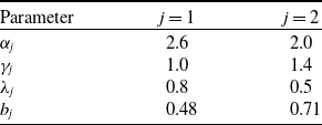
 j=1,2.

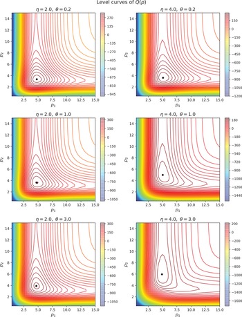
 η=2,4
 θ=0.2,1,3.
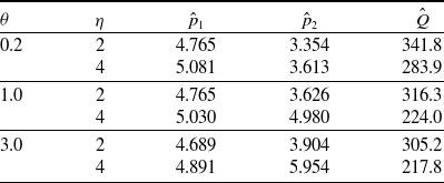
 p^=(p^1,p^2)
 Q^
 η∈{2,4}
 θ∈{0.2,1.0,3.0}
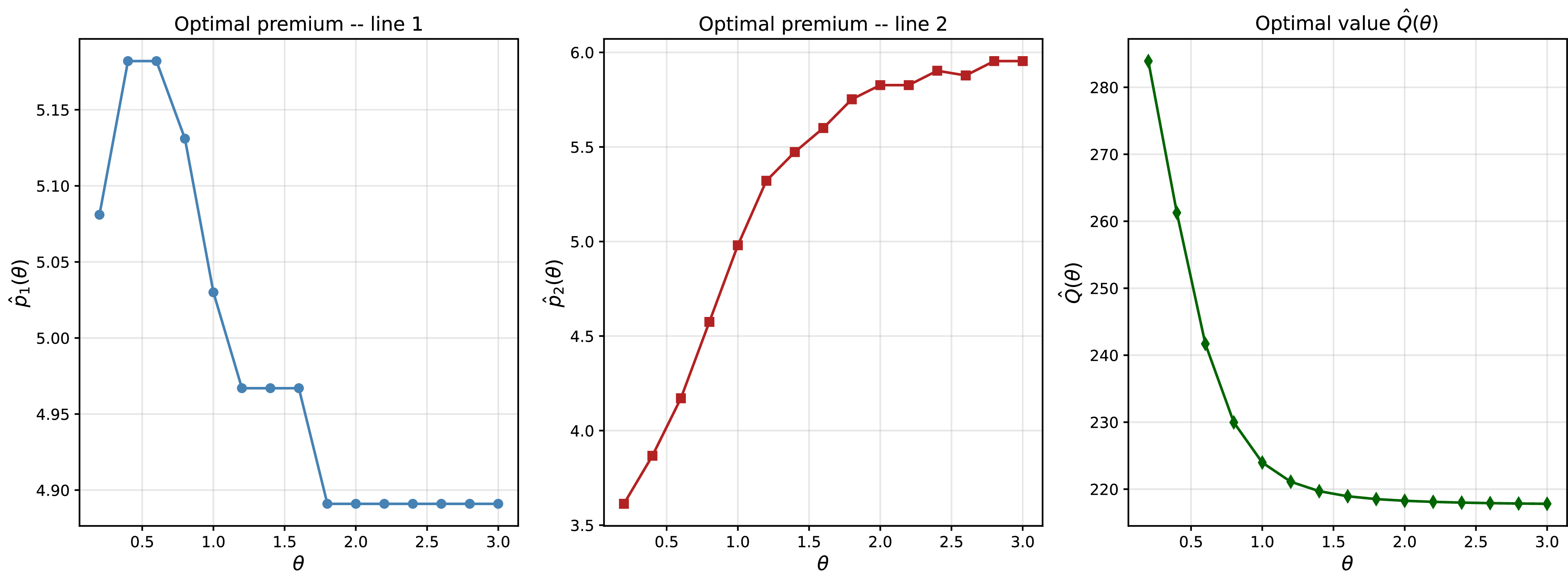
 p^(θ)=(p^1(θ),p^2(θ))
 Q^(θ)
 θ
 η=4
 [0.4,21]2
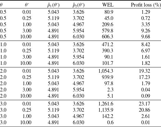
 WEL(θ,θ′)
 η=4
 R=0.04
 =(Q^(θ)−Q(p^(θ′);θ))/Q^(θ)
 θ′=θ
 =0

 Open access

