


Introduction
Bread wheat (Triticum aestivum L.) is one of the most important crops in the world, providing about 20% of the daily protein and food calories consumed globally (FAO, 2019). Wheat is the main cereal crop in Iran, which is cultivated across diverse environments, ranging from warm lowlands to cold highlands. It is expected that the demand for wheat in the country due to population growth will be increased in the coming years. In addition, the adverse effects of climate change, which will cause remarkable fluctuations in the amount and distribution of rainfall, will affect wheat productivity in the future. One of the main solutions to improve the productivity of rainfed wheat is the development of new cultivars (Foulkes et al., Reference Foulkes, Slafer, Davies, Berry, Sylvester-Bradley, Martre, Calderini, Griffiths and Reynolds2011; Hernandez-Ochoa et al., Reference Hernandez-Ochoa, Asseng, Kassie, Xiong, Robertson, Luz Pequeno, Sonder, Reynolds, Babar, Milan and Hoogenboom2018). Introducing new wheat cultivars with enhanced higher productivity and stability performance under the Mediterranean rainfed climatic conditions is found to increase the grain yield of rainfed wheat (Ludwig and Asseng, Reference Ludwig and Asseng2010; Shiferaw et al., Reference Shiferaw, Prasanna, Hellin and Banziger2011).
Wheat as other crops usually shows significant differences in terms of performance when it grows in different environments. This phenomenon is recognized as the genotype × environment (GE) interaction. The GE interaction can reduce trait heritability and the ability to predict statistically superior genotypes under contrasting environments (Gerard et al., Reference Gerard, Crespo-Herrera, Crossa, Mondal, Velu, Juliana, Huerta-Espino, Vargas, Rhandawa, Bhavani and Braun2020). Therefore, the GE interaction needs to be evaluated before introducing new cultivars that are being developed for wide recommendation and also when introducing known cultivars to new environmental conditions. An important objective of wheat breeding under the Mediterranean rainfed climates has always been to maximize productivity by increasing grain yield. The grain yield is a very complex trait which its expression relies on several factors, that is,, genetics, environment, and GE interaction (Singh et al., Reference Singh, Gupta, Gupta, Kumar, Sendhil, Tyagi, Singh, Chatrath and Singh2019; Gerard et al., Reference Gerard, Crespo-Herrera, Crossa, Mondal, Velu, Juliana, Huerta-Espino, Vargas, Rhandawa, Bhavani and Braun2020).
Several statistical methods are recommended for assessment of GE interaction in multi-environment trails (METs). Univariate methods such as Eberhart and Russell (Reference Eberhart and Russell1966), Lin and Binns (Reference Lin and Binns1988) superiority index, Shukla’s stability variance, Wricke’s ecovalence, and rank-based stability methods (Huehn, Reference Huehn1990); and multivariate methods such as additive main effects and multiplicative interaction (AMMI; Gauch, Reference Gauch2006; Gauch and Zobel, Reference Gauch and Zobel1997), and genotype main effect and GE interaction (GGE) biplot analysis (Yan et al., Reference Yan, Hunt, Sheng and Szlavnics2000) are highlighted as useful tools to assess GE interaction in different crops (Piepho, Reference Piepho1994; Annicchiarico, Reference Annicchiarico1997; Yang et al., Reference Yang, Crossa, Cornelius and Burgueno2009; Mohammadi et al., Reference Mohammadi, Armion, Zadhasan, Ahmadi and Amri2018).
AMMI analysis is now a popular statistical method which is widely used in crop breeding programs, as it can easily provide useful information regarding the complex interactions between genotypes and environments (Gauch, Reference Gauch2013). It is a hybrid method that combines both analysis of variance (ANOVA) and principal component analysis (PCA), in which the results can be used to evaluate yield stability of genotypes in MET and to determine the most suitable environments for the tested genotypes (Gauch and Zobel, Reference Gauch and Zobel1997). The outputs of AMMI analysis can be graphically presented as a biplot to evaluate the adaptability and stability performance of genotypes in METs (Gauch et al., Reference Gauch, Piepho and Annicchiarico2008). The AMMI-1 biplot shows the main effects, genotype and environment, on the abscissa; on the ordinate, it shows the first interaction principal component axis (IPCA1) (Gauch and Zobel, Reference Gauch and Zobel1997; Matus-Cádiz et al., 2003). A superior genotype as a result of AMMI analysis is one that exhibited high mean yield along with low variability across environments. In this regard, the genotypes with high mean yield and small IPCA1 could be considered as genotype for wide adaptation (Gauch and Zobel, Reference Gauch and Zobel1997; Chairi et al., Reference Chairi, Aparicio, Serret and Araus2020). Using the AMMI-2 biplot considering the both IPCA1 (on the abscissa) and the IPCA2 (on the ordinate), the interactions between genotypes and environments, interrelationships of environments, phenotypic stability, and specific and general adaptability of genotypes can be assessed. The AMMI analysis has been used in wide range of experiment with different crops (Li et al., Reference Li, Yan, Wei, Lan and Zheng2006; Singh et al., Reference Singh, Gupta, Gupta, Kumar, Sendhil, Tyagi, Singh, Chatrath and Singh2019; Chairi et al., Reference Chairi, Aparicio, Serret and Araus2020).
This study aimed at evaluating 24 winter bread wheat genotypes across 9 locations and 3 cropping seasons under rainfed conditions of Iran, in order to investigate how winter wheat grain yield was affected by GE interaction and to detect the phenotypic stability and adaptation of genotypes to rainfed climatic conditions of Iran.
Materials and Methods
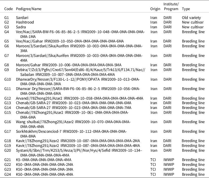
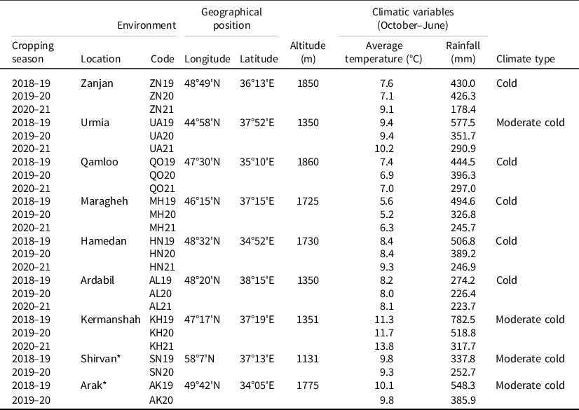
Twenty-four winter wheat genotypes consisting of 21 promising breeding lines and 3 check varieties (Table 1) were evaluated across 9 test locations (provinces), representing winter wheat national breeding program in dryland areas of Iran, for 3 cropping seasons (2018–19, 2019–20, 2020–21). More information on test locations is given in Table 2. In each environment, experimental design was a randomized complete blocks design with four replications. The size of each experimental plot was 7.2 m2 (6 rows, 6 m long, 20 cm row spacing). The sowing density was 380 seeds per m2. The fertilizers used were 50 kg N ha−1 and 50 kg P2O5 ha−1 as basal application in sowing stage. Weeds were controlled and managed by herbicides and hand weeding in each environment.
The code, name, and type of tested genotypes in the study

DARI, Dryland Agricultural Research Institute of Iran; IWWIP, International Winter Wheat Improvement Program; TCI, Turkey-CIMMYT-ICARDA.
The code, name, coordinates, and climatic variable for 25 test environments in the study

* In these two locations in 2020–21 cropping season, severe drought condition resulted in crop failure, and no data recorded.
In addition to grain yield (YLD), for each genotype days to complete of 50% heading (DHE) and physiological maturity (DMA), plant height (PLH) from the soil level to tip of spike (excluding the awns) and 1000-kernel weight (TKW) for 1000 kernels as gram was measured, but only grain yield was used for the study. The grain yield was measured as kg per plot and then converted to yield per hectare (kg ha−1) for analyses.
Data analysis
The AMMI model was performed to partition total variation in grain yield into additive main effects and their interaction, as well as partitioning multiplicative effects into interaction principal component axes (IPCAs). The AMMI analysis, as described by Gauch (Reference Gauch1992), was performed using the R software (R Core Team, 2016) with the package of GEA-R (Pacheco et al., 2015) to visualize the graphical analysis of GE interaction using the two options of AMMI-1 and AMMI-2 biplots according to the following model (Gauch, Reference Gauch1992):
 $$Yij = \mu + {g_i} + {e_j} + \mathop \sum \limits_{n = 1}^N {\lambda _n}{\gamma _{in}}{\delta _{jn}} + {\varepsilon _{ij}}$$
where Yij is the mean yield of genotype i in environment j,
 $\mu $
is the grand mean,
 ${g_i}$
is the genotypic mean deviations,
 ${e_j}$
is the environmental mean deviations, N is the number of IPCAs retained in the adjusted model,
 ${\lambda _n}$
is the square root of the eigenvalue of the IPCA axis,
 ${\gamma _{in}}$
and
 ${\delta _{jn}}$
are the IPCA scores for nth IPCA of the ith genotype and jth environment, respectively, and
 ${\varepsilon _{ij}}$
is the error.
AMMI comprises a family of models, with AMMI0 (additive model), AMMI-1, AMMI-2, and so on. The three criteria for model diagnosis are statistical significance, agricultural interpretability, and predictive accuracy. Predictive accuracy is among the most important of these criteria (Gauch, Reference Gauch2013), and it has mostly been assessed using cross-validation. The number of significant terms in the AMMI model was evaluated with the method of Gollob (Reference Gollob1968). In ANOVA, the SS for genotype (G), GE signal (GEs), and GE noise (GEn) provide a preliminary indication whether AMMI analysis will be worthwhile. The GEs can be obtained by subtracting GEn from GE. Thus, AMMI analysis is appropriate for data sets having substantial G and GEs. Especially when SS for GE is as large as that for G, as happens frequently, AMMI analysis will probably be worthwhile (Gauch, Reference Gauch2013). We applied this criterion, as suggested by Gauch (Reference Gauch2013), for the model diagnosis in AMMI.
For evaluation of yield stability of genotypes based on AMMI model, the AMMI stability value (ASV) was also applied, as described by Purchase et al., (Reference Purchase, Hatting and Van Deventer2000), as follows:
 $$ASV = \sqrt {{{\left[ {{{{S{S_{IPCA1}}}}\over{{S{S_{IPCA2}}}}}\,\left( {IPCA1scores} \right)} \right]}^2} + {{\left( {IPCA2scores} \right)}^2}\;} $$
where SSIPCA1 and SSIPCA2 are the sum of squares for the first and second IPCAs, respectively, and the IPCA1 and IPCA2 scores are the genotypic scores in the AMMI model. The lower ASV value indicates a more stable genotype across environments.
For further stability analysis, several parametric and nonparametric stability methods were also applied for the data set of 24 winter wheat genotypes grown across 25 environments. The three components of joint regression analysis including coefficient regression (bi; Finlay and Wilkinson, Reference Finlay and Wilkinson1963), variance deviation from regression (S2 d; Eberhart and Russell, Reference Eberhart and Russell1966), and coefficient of determination (R2; Pinthus, Reference Pinthus1973), as well as coefficient of variability (CV, Francis and Kannenberg, Reference Francis and Kannenberg1978), Shukla’s Stability variance (σ2 sh; Shukla, Reference Shukla1972), Wricke’s ecovalence (W2; Wricke, Reference Wricke1962), superiority measure (Pi) of Lin and Binns (Reference Lin and Binns1988), and two nonparametric stability statistics of S1 (i) and S2 (i) (Huehn, Reference Huehn1990) were applied for stability analysis.
Results
Weather conditions
The amount and monthly distribution of rainfall varied from location to location and year to year (Table S1), provided different growth conditions that led to a wide range of grain yield potentialities. The rainfalls recorded varied from 178.4 mm (corresponding to Zanjan location in 2020–21) to 782.5 mm (corresponding to Kermanshah location in 2018–19). For a wheat crop with a reasonable grain yield under rainfed condition, about 400 mm is adequate. Ten out of 25 test environments received rainfalls higher than 400 mm, although most of the rainfall received in winter and was not effectively used by crops. In all environments, the rainfall received during flowering and grain filling period was not sufficient and crops experienced severe terminal drought. The average annually temperatures varied between 5.5 and 13.1°C, while average minimum monthly temperature was −5.9°C recorded in January (Maragheh location in 2018–19) and average maximum monthly temperature was 25.3°C recorded in June (Kermanshah location in 2018–19). More details on monthly and average annual temperature for test locations across years are given in Table S2.
ANOVA and variation in genotype’s performance
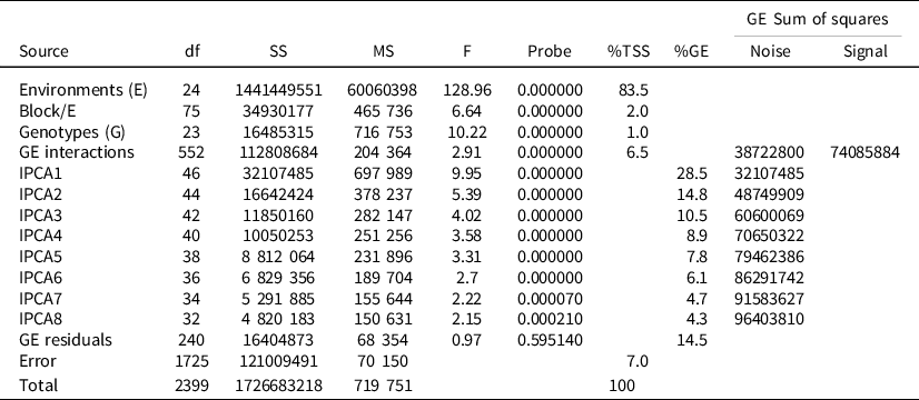
The results of AMMI ANOVA showed that the environment, as the main source of variation in grain yield (accounting for 83.5% of total variation), had highest impact on the performance of genotypes (Table 3). Genotype effect explained only 1.0% compared to GE interaction effect that captured 6.5% of the total variation. This indicates that the size of GE interaction was about 6.5 times larger than genotype effect, suggesting strong crossover GE interaction. The low percentage of variance explained by genotype may be due to the fact that the genetic materials used in this study already are selected as top-yielding materials through wheat breeding program in previous years. Similar results also reported by other studies (Bocianowski et al., 2019; Chairi et al., 2020; Mohammadi et al., Reference Mohammadi, Sadeghzadeh, Poursiahbidi and Ahmadi2021) that the genotype portion in MET has been known to be the smallest among all sources of variation. The AMMI model further partitioned the interaction sum of square into eight significant IPCAs (Table 3), which captured 85.6% of the total GE interaction.
AMMI analysis of variance for grain yield of 24 winter wheat genotypes across 25 environments

%TSS, percent relative to total sum of squares; %GE, percent relative to GE interaction.
Model diagnosis is one of the most important steps in AMMI analysis. As described by Gauch (Reference Gauch2013), in most published papers related to AMMI analysis, no model diagnosis was performed. Instead, AMMI-1 and AMMI-2 usually are taken as an automatic default, because convenient two-dimensional graphs can be based on such models. In contrast, a graphically represented AMMI analysis enables selection of stable and high-yielding genotypes for variable environments, as well as genotypes with specific adaptability. This information can be captured only through the AMMI biplots such as AMMI-1 and AMMI-2 biplots. The postdictive success through the multiplicative terms indicated eight significant IPCAs, which indicated AMMI-8 as the best model, while the predictive success through GEs method suggested AMMI-4 as the best model, as the cumulative sum of squares for the first four PCs is close to sum of squares of GE signal (SSGEs) (Table 3). According to Gauch (Reference Gauch2013), early IPCAs capture a signal, whereas late IPCAs capture noise; discarding noise improves accuracy and increases repeatability.
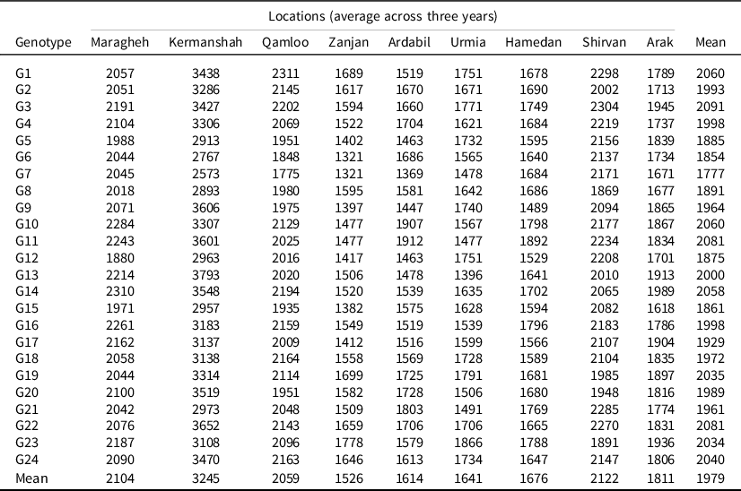
The results of ANOVA showed that field trials significantly affected by environmental conditions mainly weather conditions. The mean yields of genotypes ranged from 1777 kg/ha (corresponding to genotype G7) to 2091 kg/ha (corresponding to genotype G3), with an average value of 1979 kg/ha throughout the 25 test environments (Table 4). The location mean yield varied from 1526 kg/ha (corresponding to Zanjan location) to 3245 kg/ha (corresponding to Kermanshah location). The other locations with low productivity were Ardabil (1614 kg/ha) and Urmia (1641 kg/ha). The highest mean genotypic yields per location also ranged from 1321 kg/ha for genotypes G5 and G6 in Zanjan location to 3793 kg/ha for genotype G13 in Kermanshah location. This shows high difference in genotypes responses to locations across years that can be supported by the 6.5 times larger effect of GE interaction compared to genotype effect (Table 3).
Mean yields (kg/ha) of 24 winter wheat genotypes across three cropping seasons

AMMI biplots analysis
The stability of genotypes, environments, and specific GE interactions can be investigated graphically through the AMMI-1 biplot (Figure 1). Genotypes with high main effects and low IPCA score are considered as ideal genotypes (Gauch and Zobel, Reference Gauch and Zobel1997). The environments KH20 and KH19 with the highest mean yield expressed high contribution to GE interaction, while the environments HN21, UA20, ZN21, and AL21 with lowest productivity showed the least contribution to GE interaction, as they had the IPCA1 scores near to zero. The environments HN20, QQ20, MH19, and SN19 with productivity higher than grand mean expressed low contribution to GE interaction, while environments SN19, HN19, and AK19 with lower productivity than grand mean exhibited higher contribution to GE interaction. The genotypes G13 and G14 with highest positive IPCA1 scores and genotypes G21, G12, G5, and G18 with highest negative IPCA1 scores were identified as unstable genotypes showing different adaptation to environments. The genotypes G3, G23, G22, G10, and G19 showed highest mean yield with least IPCA1 scores, while G7, G6, and G11 expressed lowest performance and stability, and G14 and G11 with high productivity showed highest instability and tend to specific adaptation to some environments corresponding to Kermanshah location.

To further evaluate the GE interaction, the AMMI-2 biplot was constructed based on the first two IPCAs and captured 43.2% of total GE interaction variation. AMMI-2 biplot depicts the spatial pattern of genotypes and environments based on the first two IPCAs scores, which helps in visual interpretation of the GE interaction patterns and identification of genotypes or environments that contribute to low, medium, or high level of interaction (Figure 2). The environments KH20 and KH19 with the longest vectors tended to highest contributing to GE interaction and presenting highest discriminating ability among environments. The environments SN19, UA19, HN19, AK19, SN20, and MH21 with moderate vectors tended to high contribution into GE interaction, while other environments were not most informative in genotype discrimination due to short vectors. The cosine angle between two environment vectors shows correlation between two environments. The environments with acute angle are positively correlated in ranking of genotypes. The environments KH20, KH19, and AK20 positively correlated and the genotypes G13, G20, G2, G14, and G11 positively interacted with these environments, while the genotypes G7, G4, G21, G50, G12, and G15 negatively interacted with these environments. KH20 and KH19, characterized as favorable environments, were strongly correlated and the genotypes G13, G14, G9, G20, and G11 specifically adapted to these environments. Environments SN19 and UA19 were positively correlated and genotypes G12, G8, G15, and G4 positively interacted with these environments. Environments HN19, AK19, AL19, and AL20 showed positive correlations with each other and were same in discriminating of genotypes G21, G6, G7, G5, and G17. Environments MH21 and SN20 closely associated with ranking of genotypes and genotypes G10 and G16, and G11 and G14 positively interacted with these environments. Genotypes G14, G13, G7, G10, and G6 showed most extreme values of both IPCA1 and/or IPCA2 scores, indicating they were most contributing to GE interaction and tend to specific adaption to particular environments. For example, G14 showed specific adaptation to the favorable environment KH20, while G7, G6, and G21 most adapted to environments HN19 and AK19, and genotype G22 most adapted to favorable environment KH19.

The positively significant (p < 0.01) correlation coefficients for grain yield were observed for the following pair of test environments: ZN19-ZN20 (r = 0.79), AL21-ZN20 (r = 0.84), HN20-ZN20 (r = 0.71), AK20-ZN20 (r = 0.69), HN21-ZN21 (r = 0.67), QQ21-UA20 (r = 0.89), QQ19-UA21 (r = 0.67), QQ19-UA21 (r = 0.67), QQ20-UA21 (r = 0.62), AK20-QQ19 (r = 0.89), AL21-QQ19 (r = 0.70), AK20-QQ20 (r = 0.61), HN20-MH19 (r = 0.65), MH21-MH19 (r = 0.65), HN21-MH19 (r = 0.60), KH20-MH21 (r = 0.72), AL21-HN20 (r = 0.62), KH20-HN20 and HN20-HN21 (r = 0.59), KH19-HN21 (r = 0.58), AK20-AL21 (r = 0.79), KH20-AL21 (r = 0.60), and KH20-AK20 (r = 0.74) (Figure 3). These results show some similarities among environments in genotypes ranking, which should be considered in future studies to save costs and resources. In contrast, negative significant correlations (p < 0.01) were observed for grain yield for the following pair of test environments: AK19-ZN19 (r = −0.54), AK19-ZN20 (r = −0.64), MH21-UA19 (r = −0.59), AL20-UA20 (r = −0.52), AK19-QQ20 (r = −0.58), AL20-QQ21 (r = −0.54), KH19-AK19 (r = −0.59), SN19-AK20 (r = −0.53), AK20-AK19 (r = −0.54), and SN19-KH20 (r = −0.56) (Figure 3).
Heat map for correlation coefficients between mean yields observed in different environments. Critical values for significant at p < 0.01 is 0.520 and at p < 0.05 is 0.411. For environment names, see Table 2.

Performance of genotypes based on stability methods
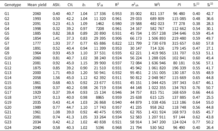
The genotypes showed significant differences (p < 0.01) in grain yield across environments, showing that the performance of genotypes varied across environments leading to significant GE interaction (Table 3). The mean yield and stability values for 24 winter wheat genotypes across 25 rainfed environments are presented in Table 5. Taking genotypic mean performance as a first parameter for assessment, the genotypes G3, G22, G11, G10, and G1 expressed highest mean yield across environments, while G7 followed by G6, G15, G12, and G5 exhibited poor yields across environments. ASV expressed high variations in yield stability among the 24 tested genotypes. According to ASV, a genotype with ASV value close to zero can be regarded as stable genotype. Accordingly, genotype G18 followed by G3, G4, G16, and G17 showed highest yield stability, while the genotype G7 followed by G13, G14, G6, and G21 was unstable. Genotypes G3, G4, and G16 with mean yield higher than grand mean expressed highest stability based on ASV, showing high level of combination of mean yield and stability.
The mean yield and stability values for 24 winter wheat genotypes across 25 rainfed environments

Genotypes G13, G11, G14, G9, and G20 with highest regression coefficients (b i) showed better adaptation to favorable environments, whereas G7, G6, G5, G12, and G21 with lowest regression coefficients and mean yields less than grand mean, specifically adapted to harsh conditions. Genotype G3 with the highest mean yield had the lowest variance in regression deviation (S2di) and G7 with lowest mean yield expressed maximum S2di (Table 5). Genotype G3 exhibited a good combination of yield and stability followed by G23 that ranked second for the lowest S2 di and ranked fifth for yield performance.
According to the coefficient of determination (R2), genotypes G3, G24, G4, G2, and G18 with highest R2 values expressed highest stability, whereas genotypes G23, G14, G6, G21, and G7 with the lowest R2 values showed highest instability. The CV parameter was lowest for genotypes G4, G7, G5, G21, and G12 with lowest mean yield, whereas the genotypes G13, G9, G14, G11, and G20 with the highest mean yields expressed highest CV values and identified as unstable genotypes (Table 5). For the both methods of Wricke’s ecovalence (W2 i) and Shukla’s stability variance (σ2 i), genotypes G3, G24, G4, G18, and G2 were identified as most stable genotypes, while G7, G13, G14, G11, and G6 contributed for highest GE interaction and identified as unstable genotypes. Genotypes G3, G11, G1, G24, and G22 with the lowest values of superiority measure (Pi) identified as stable genotypes with high-yielding performance, while the G7, G6, G15, G12, and G5 exhibited highest values of Pi and identified as unstable genotypes with low productivity. Using the nonparametric stability statistics, genotypes G3, G1, G24, G18, and G8 with lowest values for Si(1) expressed highest stability and G23, G16, G15, G17, and G21 with lowest values showed most instability. Genotype G18 followed by G24, G8, G3, and G4 with lowest values of Si(2) identified as stable genotypes and G7 followed by G11, G19, G9, and G16 identified as unstable genotypes.
Interrelationships among mean yield and stability parameters
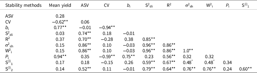
The Spearman’s rank correlations between genotypic mean yields and stability parameters are presented in Table 6. The Pi and bi expressed positive and significant correlation (p < 0.01) with mean yield, while CV exhibited negative and significant correlations (p < 0.01) with mean yield. The ASV significantly correlated (p < 0.01) with stability statistics of S2 di, R2 i, σ2 sh, W2i, and nonparametric statistic of S(i) 2. The CV, in addition to mean yield, showed negative and significant relationships (p < 0.01) with Pi and bi. The stability statistics of S2 di, R2, σ2 sh, W2 i, S(i) 1, and S(i) 2 were positively and significantly correlated with each other, showing they are given similar ranks in genotypes selection. W2i and σ2 sh were identical in genotypes ranking as they were showed correlation coefficient equal to unit (r = 1.0).
Spearman’s rank correlation between mean yield and parametric and nonparametric stability measures for 24 winter wheat genotypes across 25 environments

*,**Significant at 5% and 1% level of probability, respectively.
ASV, AMMI stability value; CV, coefficient of variation; bi, regression coefficient; S2 di, variance in regression deviations; R2, coefficient of determination; σ2 sh, Shukla’s stability variance; W2 i, Wricke’s ecovalence; Pi, superiority index; S(i) 1 and S(i) 2, rank-based stability statistics.
Discussion
In this study, there existed significant grain yield variation in the case of genotype, environment, and GE interaction main effects. The tested genotypes are from the winter wheat breeding program of DARI, Iran, and are evaluated as promising breeding lines in the targeting rainfed Mediterranean regions for identifying high-yielding and stable genotypes. The test locations for this study are popular winter wheat growing regions that fall under highland rainfed areas with contribution for more than 70% of rainfed wheat production in Iran (Iran-AgriStat, 2020). However, in this area rainfall is the most constraint of crop growth and productivity, leading to failure crops in some years (Mohammadi et al., Reference Mohammadi, Armion, Zadhasan, Ahmadi and Amri2018). The crop performance was significantly (p < 0.01) affected by environmental condition, which accounted for 83.5% of total variation (Table 3); a near value to the 84.3% and 85% obtained from previous studies in durum wheat in Iran (Mohammadi et al. Reference Mohammadi, Armion, Zadhasan, Ahmadi and Amri2018, Reference Mohammadi, Sadeghzadeh, Poursiahbidi and Ahmadi2021).
However, selection for grain yield improvement is a very complex phenomenon and should be considered in accounting genotypes along with the environmental interactions. The models underling stability analysis will help in investigating the GE interaction and help in identifying the stable and high-yielding genotypes as well as adapted genotypes for targeting regions (Gauch and Zobel, Reference Gauch and Zobel1997; Gauch, Reference Gauch2006; Yan et al., Reference Yan, Hunt, Sheng and Szlavnics2000).
The GE interaction analysis in multi-environment yield trials is crucial for assessment, selection, and recommendation of new crop varieties. For this propose, AMMI models are widely used in breeding programs of different crops such as wheat (Singh et al., Reference Singh, Gupta, Gupta, Kumar, Sendhil, Tyagi, Singh, Chatrath and Singh2019; Chairi et al., Reference Chairi, Aparicio, Serret and Araus2020). The high-yielding and stable genotypes were identified that could be explored for cultivar recommendation as well as for pre-breeding objectives for developing promising wheat genotypes. AMMI biplots provided useful information on genotype and environment relationships. In this regard, the cosine of the angle between the environments ranged from negative (angle > 90°) to positive (angle < 90°) correlations, showing environments with positive correlation are similar in ranking of genotypes and vice versa (Yan et al., Reference Yan, Hunt, Sheng and Szlavnics2000). The Pearson’s correlation analysis between environments was in accordance with the AMMI biplots results. Similar reports on positive and negative correlation between environments are already reported in the analysis of MET data in different crop species (Mohammadi et al., Reference Mohammadi, Armion, Zadhasan, Ahmadi and Amri2018; Olivoto et al., Reference Olivoto, Lucio, da Silva, Marchioro, de Souza and Jost2019; Katsenios et al., Reference Katsenios, Sparangis, Leonidakis, Katsaros, Kakabouki, Vlachakis and Efthimiadou2021). The negative correlation between environments indicates the presence of high cross over GE interaction (Ebdon and Gauch, Reference Ebdon and Gauch2002).
AMMI analysis revealed the major contribution of the environmental effects followed by GE interaction and genotypic effects. Based on the performance of genotypes across different environments, AMMI-1 classified the genotypes G3, G23, G22, G10, and G19 with highest mean yield and stability performance, and genotypes G7, G6, and G11 expressed lowest performance and stability, while genotypes G14 and G11 with high mean yield and highest instability tend to specific adaptation to some environments (i.e., Kermanshah location). Similar trends in classification of genotypes by AMMI-1 biplot are already reported in other studies (Singh et al., Reference Singh, Gupta, Gupta, Kumar, Sendhil, Tyagi, Singh, Chatrath and Singh2019; Yohane et al., Reference Yohane, Shimelis, Laing, Mathew and Shayanowako2021). Furthermore, using the AMMI-1 biplot the highly interactive environments (KH20, KH19, and SN19) and genotypes (G7, G13, G14, and G6) were identified.
Using the AMMI-2 biplot, the precise adaptation of genotypes to suitable environments could be graphically visualized. The environments KH20, KH19, and AK20 were more appropriate for the genotypes G13, G20, G2, G14, and G11, while the genotypes G13, G14, G9, G20, and G11 expressed the high-yielding potential in environments KH20 and KH19; genotypes G12, G8, G15, and G4 showed positive interaction with environments SN19 and UA19, whereas environments HN19, AK19, AL19, and AL20 were suitable for the genotypes G21, G6, G7, G5, and G17; and the genotypes G10, G16, G11, and G14 exhibited highest adaptation to environments MH21 and SN20. Singh et al., (Reference Singh, Gupta, Gupta, Kumar, Sendhil, Tyagi, Singh, Chatrath and Singh2019) in wheat and Katsenios et al., (Reference Katsenios, Sparangis, Leonidakis, Katsaros, Kakabouki, Vlachakis and Efthimiadou2021) in maize also reported the better performance of particular genotypes for each or a group of environments under study. Based on ASV, genotypes G3, G4, and G16 with high mean yield expressed highest stability, showing high level of combination of mean yield and stability in these genotypes.
Integrating univariate stability methods with multivariate methods allows breeders to select stable genotypes and help with improving recommendations to the growers (Mohammadi et al., Reference Mohammadi, Sadeghzadeh, Poursiahbidi and Ahmadi2021). The lowest values of superiority index (Pi) for genotypes G3, G11, G1, G24, and G22 revealed a minimum distance between the performance of these genotypes and the maximum response observed across environments. This shows a proportional increase in the performance of these genotypes in response to the enhancement of the variable environments, thus resulting in greater stability (Lin and Binns, Reference Lin and Binns1988), which is related to dynamic concept of stability (Becker and Leon, Reference Becker and Leon1988).
The lower values of the statistics W2 i, σ2, R2, ASV, and S2 di for genotypes G3, G24, G4, G18, and G2 indicate that they are stable genotypes, which are related to static concept of stability and often are not correlated with mean yield (Becker and Leon, Reference Becker and Leon1988). These results are in accordance with the correlation analysis between stability methods with grain yield (Table 6). The Pi positively correlated with mean yield, showing this stability method is strongly related to dynamic concept of stability which is in accordance with other reports (Mohammadi and Amri, 2008; Scapim et al., 2012; Temesgen et al., Reference Temesgen, Keneni, Sefera and Jarso2015). In contrast, the stability methods W2 i, σ2, R2, ASV, and S2 di were not associated with mean yield that confirms these methods are related to static concept of stability, that can be confirmed with other studies (Mohammadi and Amri, 2008; Scapim et al., 2012; Temesgen et al., Reference Temesgen, Keneni, Sefera and Jarso2015). As an interesting result, the AMMI-based stability value showed a positive and significant correlation (p < 0.01) with the most stability methods such as W2 i, σ2 i, R2 i, S2 di, and S2 (i). These results also indicate that the selection for stability based on AMMI model (i.e., ASV) might lead to selection of genotypes with static stability.
Conclusion
This study provides a valuable data set (24 winter wheat genotypes, 9 representative testing locations for wheat productivity and 3 years) with new findings that can be explored in wheat breeding program. AMMI analysis suggests that an increase in yield can be accomplished by recommending genotypes for both specific and wide adaptation strategies. The positive interaction of particular genotypes in environments with favorable/unfavorable climatic conditions can be valuable for the scientific community. This study revealed that the genotypes G3, G23, G22, G10, and G19 with highest mean yield and stability performance were highly suitable for all the environments, and genotypes G7, G6, and G211 were particularly adapted to unfavorable environments, while G14, G13, G20, and G9 were suitable for favorable environments. In the present study, partitioning and interpretation of the GE interaction and phenotypic stability for grain yield were evaluated through the AMMI and several stability methods. Both approaches were found to be efficient methods in exploring the GE interaction in multi-environment yield trials. The AMMI biplots were able to identify high-yielding and stable wheat genotypes with high genetic capability to adapt to drought condition. However, in crop breeding programs both mean yield and stability should be considered simultaneously to exploit the useful effects of GE interaction and to make the selection of favorable genotypes more precise.
Supplementary material
To view supplementary material for this article, please visit https://doi.org/10.1017/S0014479722000345
Acknowledgements
The authors thank the two reviewers and the Editor of Experimental Agriculture for comments and corrections to the manuscript.
Conflict of Interest
The authors declare that they have no conflicts of interest.