1. Introduction
The concentric flow formed by two immiscible fluids within a pipeline is referred to as core–annular flow (CAF), which is a prototypical yet relatively simple flow phenomenon. Industrial applications are often associated with the transportation of high-viscosity liquids. In such systems, a layer of low-viscosity fluid (e.g. water) may be used to coat a high-viscosity fluid (e.g. oil), which reduces frictional resistance and energy consumption. Hence, a CAF comprises a crucial lubricating flow regime in the pipeline transportation of high-viscosity oils (Charles, Govier & Hodgson Reference Charles, Govier and Hodgson1961; Joseph et al. Reference Joseph, Bai, Chen and Renardy1997). The mechanism of reducing the resistance and energy consumption will partially or completely fail when the ideal annular flow structure is destroyed. The interfacial stability of annular flows has become the subject of many studies. Thus far, numerous studies have attempted to clarify the underlying physical mechanisms of a CAF. Investigations of its drag-reducing characteristics can be found in Charles et al. (Reference Charles, Govier and Hodgson1961), Prada & Bannwart (Reference Prada and Bannwart2001), Ooms & Poesio (Reference Ooms and Poesio2003) and many others. A comprehensive review of the drag reduction characteristics is presented in Xie et al. (Reference Xie, Jiang, Lin, Zhang, Gui and Xiang2023). These studies have shown that high- and low-viscosity fluids with different densities can form various flow regimes within pipelines. In horizontal pipe flows, where the aqueous phase forms a thin lubricating layer surrounding the oil core, the pressure drop can be reduced significantly compared with those of single-phase oil flows and by up to 90 % in some cases (Bensakhria, Peysson & Antonini Reference Bensakhria, Peysson and Antonini2004).
The rapid development of computational techniques has enabled numerical simulations to provide new insights into the mechanisms governing a CAF. Saurel & Pantano (Reference Saurel and Pantano2018) proposed a series of governing models and numerical schemes for capturing two-phase interfaces, which not only improved the accuracy of interface tracking but also facilitated a detailed analysis of the instability mechanisms induced by interfacial disturbances. These advances have provided a robust numerical framework for investigating the coupling between the interface and vortex core in CAFs with strong density contrasts. Moreover, direct numerical simulations have been employed for studying the interface morphology and pressure-drop characteristics of a turbulent CAF, confirming the effect of gravity-induced asymmetry in the annular film on drag reduction (Kim & Choi Reference Kim and Choi2024). Furthermore, the linear stability of CAF interfaces has garnered considerable attention, and this can be traced back to previous research studies (Preziosi, Chen & Joseph Reference Preziosi, Chen and Joseph1989; Bai, Chen & Joseph Reference Bai, Chen and Joseph1992; Kouris & Tsamopoulos Reference Kouris and Tsamopoulos2001 and many others). A comprehensive review has been presented in Ghosh et al. (Reference Ghosh, Mandal, Das and Das2009). The stability analysis showed that a stable CAF exists only in the range in which the oil core is dominant and the lubricating layer thickness is moderate. An annular lubricating layer with an extremely low-viscosity ratio can easily trigger an axisymmetric long-wave instability. Furthermore, in horizontal pipelines, gravity causes denser water to settle at the bottom and the less-dense oil phase to migrate upward, resulting in asymmetric stratification across the pipe diameter. This is in contrast to vertical pipelines, where buoyancy effects manifest along the axial direction, thereby leading to rising or sinking motions. Therefore, the non-uniform effect of gravity on stratified two-phase fluids with different densities in horizontal pipelines cannot be ignored (McCaslin & Desjardins Reference McCaslin and Desjardins2014). The eccentric positioning of the oil core caused by gravity must be counterbalanced by the radial pressure induced by interfacial waves. The hydrodynamic lubrication theory suggests that lubrication forces may offset buoyancy in a CAF exhibiting ‘snake’ waveforms. However, this is not the case in ‘bamboo’ wave regimes (Ooms & Poesio Reference Ooms and Poesio2003). At low Reynolds numbers (definition of
 ${\textit{Re}}_{z}$
is given in § 2), the interfacial tension can drive capillary instabilities. Chen & Joseph (Reference Chen and Joseph1991) demonstrated that, beyond a certain critical Reynolds number, inertial effects can completely suppress such long-wave instabilities. Overall, the parameter space required to maintain a stable CAF is narrow.
This study focuses on investigating a swirling CAF in horizontal pipelines. Research on the formation of a swirl within pipes can be traced back to the work of Isaac & Speed (Reference Isaac and Speed1904), who designed a straight pipe with an internal helical structure to induce vortical motion. This pioneering idea has since inspired new design strategies for axially swirl-induced two-phase separation devices (Xu et al. Reference Xu, Zhang, Zhao, Jiang, Liu and Xia2021). Recently, Wu et al. (Reference Wu, Liao, Qin, Zhang and Wang2025) introduced an adjustable-speed rotating element within a pipeline segment for imparting circumferential rotation to an oil–water mixture. Even under low flow rates, a stable film of low-viscosity water formed along the pipe wall, which effectively isolates the oil core and suppresses interfacial disturbances in the oil–water mixing layer. This configuration led to the formation of a swirling CAF, which has been employed for measuring water-cut and flow rates in oil-well extraction systems. The presence of azimuthal rotation gives rise to a swirling vortex core within the flow, introducing additional complexity to its stability behaviour (Jacquin & Pantano Reference Jacquin and Pantano2002; Yang & Pullin Reference Yang and Pullin2011; Shen et al. Reference Shen, Yao, Hussain and Yang2023). Moreover, the introduction of circumferential rotation to immiscible two-phase flows can lead to a broader spectrum of interfacial instability modes, as it incorporates not only the instability induced by viscous shear in stratified fluids, but also the centrifugal instability (CTI) associated with rotation (Pillai & Narayanan Reference Pillai and Narayanan2018; Sarma & Mondal Reference Sarma and Mondal2021a , Reference Sarma and Mondalb ).
Although the stability analyses of a swirling CAF are scarce, valuable insights can be drawn from the investigations of interfacial instabilities in rotating two-phase systems. Gallaire & Chomaz (Reference Gallaire and Chomaz2003) used linear stability analysis to study the linear stability of a rotating jet system, which reveals that the synergistic effect of circumferential shear and CTI mechanisms significantly change the mode selection rule. In the non-swirl state, the axisymmetric instability mode is governed by the Kelvin–Helmholtz instability (KHI) induced by axial shear. The CTI caused by the centrifugal force gradient begins to activate a large number of spiral modes with an increase in rotation intensity. Similarly, Boguslawski & Wawrzak (Reference Boguslawski and Wawrzak2020) analysed the local stability of an annular jet and revealed that the spatiotemporal growth rate of the spiral mode is governed by reflux velocity (i.e. the reverse flow velocity near the central axis of the annular jet) and swirl intensity. An increase in the reflux velocity markedly enhances absolute instability, whereas an increase in swirl intensity leads to an increase in the disturbance frequency via the centrifugal effect. These findings provide a direct theoretical analogy for spiral stabilities observed in a CAF. The instability mode resembles the spiral dynamic mode of classical rotating jets when the velocity gradient of the inner and outer layers and centrifugal effects act on the immiscible two-phase interface; the circumferential momentum transport caused by the swirl is the core mechanism triggering global absolute instability.
Energy-based analysis offers a deeper perspective for understanding the interfacial stability of immiscible two-phase flows. Unlike conventional modal analysis, which focuses on eigenvalue growth rates, energy analysis tracks the temporal evolution of perturbation energy to capture transient energy amplification processes that could otherwise be overlooked. The essential value of an energy budget analysis lies in its ability to distinguish between the energy components that promote the growth of interfacial disturbances and those that suppress them, thereby elucidating the physical mechanisms governing interfacial instability. Related research can be traced back to Hu & Joseph (Reference Hu and Joseph1989), who used linear stability theory for studying the transient energy growth of an oil–water CAF. This study revealed the effects of surface tension, viscosity ratio and gap ratio on transient instability, thereby providing a theoretical basis for parameter optimisation in lubrication and transportation design. More recently, Orazzo et al. (Reference Orazzo, Coppola and de Luca2014) studied the linear stability of a CAF and showed that three-dimensional spiral disturbances exhibit strong transient disturbance energy amplification when the axial wavenumber is approximately zero. The Reynolds number of the annular phase was defined based on the velocity along the flow axis, the radius of the core phase and the properties of the annular layer. The energy analysis indicated that the mechanism responsible for this transient amplification occurred within the annular layer and was closely linked to the Reynolds number and thickness of the annular region. Furthermore, Barmak et al. (Reference Barmak, Gelfgat, Ullmann and Brauner2019) extended the energy norm to include gravitational potential energy and interfacial capillary energy and studied horizontal and inclined two-phase stratified channel flows. They found that the transient release of gravitational potential energy can supply energy to the disturbance, particularly under conditions of strong gravitational effects.
Despite extensive studies on the stability mechanisms of a CAF, investigation of a CAF with circumferential rotation remains largely unexplored, particularly regarding its intrinsic instability mechanisms. The importance of a circumferentially swirling CAF is becoming increasingly apparent with growing demands in the energy sector (Wang et al. Reference Wang, Wang, Niu, Wei and Liu2017; Wu et al. Reference Wu, Liao, Qin, Zhang and Wang2025). In this study, a linear temporal stability analysis was conducted based on a model of an immiscible two-phase swirling CAF. The analysis incorporates the effects of gravity, interfacial tension, axial and azimuthal shear stresses, and centrifugal forces on interfacial disturbances. In addition, an energy budget model that included gravitational potential energy was developed for clarifying dominant physical mechanisms responsible for the instability of swirling CAF interfaces. The remainder of this paper is organised as follows. In § 2 we outline the physical and numerical methodology, including the governing equations, boundary conditions and solution procedure. The results and discussion related to interfacial stability are presented in § 3, where dispersion relations and a parametric study are discussed. The underlying instability mechanisms of the interface are examined in § 4. The main conclusions are summarised in § 5.
2. Methodology
2.1. Linear interfacial stability analysis
Figure 1 presents a schematic of the physical model used in this study. We consider two incompressible and immiscible Newtonian fluids flowing through a circular pipe with radius
 $ r_2$
. The initial flow state of the two fluids is set as a CAF, where the fluid with density
 $ \rho _1$
occupies the inner radius
 $ r_1$
and is surrounded by the fluid with density
 $ \rho _2$
. The flow is described using cylindrical coordinates
 $ r$
,
 $ \theta$
and
 $ z$
, which corresponds to velocity components
 $ v$
,
 $ w$
and
 $ u$
, respectively. For each phase, the velocity may be expressed as
 $\boldsymbol{U^*_i(r)}=U^*_i(r)\boldsymbol{e}_z+W^*_i(r)\boldsymbol{e}_\theta$
, where
 $U^*_i(r)$
and
 $W^*_i(r)$
(
 $i=$
1, 2) denote the dimensional axial and azimuthal velocity components, respectively.
The parameters illustrated in figure 1 are as follows: the radius
 $r_2$
of the pipeline is set to 10 mm and
 $r_1$
is a variable employed to analyse the proportion of the two phases. We select white oil and water as the core phase and the annular phase, respectively. Accordingly, the density
 $\rho _1$
of the core phase is 860 kg m
 $^{-3}$
with a dynamic viscosity
 $\mu _1$
of 0.02 Pa s, and the density
 $\rho _2$
of the annular phase is 998 kg m
 $^{-3}$
with a dynamic viscosity
 $\mu _2$
of 0.001 Pa s, surface tension
 $\sigma$
is 0.042 N m
 $^{-1}$
and acceleration due to gravity
 $g$
is 9.81 m s
 $^{-2}$
.
Schematic of the initial motion state of two fluids in a cylindrical coordinate system (
 $r$
-
 $\theta$
-
 $z$
). A swirling motion is applied at the inlet that corresponds to the Rankine vortex. The origin of the coordinate system is set at the centre of the entrance.

We employ the linear stability theory to analyse the interfacial stability of incompressible and immiscible two-phase spiral annular flows in a horizontal pipe considering gravity. The characteristic length, velocity and time are selected as
 $ r_1$
,
 $ W^*_{max}$
and
 ${r_1}/{W^*_{max}}$
, respectively, where
 $W^*_{max}$
represents the azimuthal velocity at the interface between the core and annular phases. Therefore, dimensionless parameters include the rotational Reynolds number
 ${\textit{Re}} = {\rho _1 W^*_{max} r_1} / {\mu _1}$
, axial Reynolds number
 ${\textit{Re}}_{z} = {\rho _1 \bar {U_1}r_1} / {\mu _1}$
, Weber number
 ${\textit{We}} = {\rho _1 W^{*2}_{max} r_1} / {\sigma }$
, Ohnesorge number
 ${\textit{Oh}} = \sqrt {We}/Re = \mu _1/{\sqrt {\rho _1 \sigma r_1}}$
, Froude number
 $Fr = W^*_{max}/{\sqrt {r_1g}}$
, density ratio
 $J = \rho _2 / \rho _1$
, viscosity ratio
 $N = \mu _2/\mu _1$
and radius ratio
 $ R = r_2/r_1$
. We first model the incompressible, immiscible two-phase fluid independently, and the dimensionless governing equation for this fluid can be expressed as
 \begin{align} \boldsymbol{\nabla }\boldsymbol{\cdot }\boldsymbol{u}_i &= 0, \\[-9pt] \nonumber \end{align}
 \begin{align} \frac {\partial \boldsymbol{u}_i}{\partial t} + \boldsymbol{u}_i \boldsymbol{\cdot }\boldsymbol{\nabla }\boldsymbol{u}_i = - \left ( \frac {1}{J} \right )^{\delta _{2i}} \boldsymbol{\nabla }p_i &+ \left ( \frac {N}{J} \right )^{\delta _{2i}} \frac {1}{Re} {\nabla} ^2 \boldsymbol{u}_i+\frac {1}{Fr^2}\boldsymbol{\gamma _i}, \end{align}
where
 $\boldsymbol{u_i}(=v_{i}\boldsymbol{e_r}+w_{i}\boldsymbol{e_{\theta }}+u_{i}\boldsymbol{e_z})$
,
 $\delta _{2i}$
,
 $i\,(= 1,2)$
, and
 $\boldsymbol{\gamma _i}$
represent the velocity component in cylindrical coordinates (
 $r, \theta , z$
), Kronecker symbol, core and annular phases, and direction of gravitational acceleration, respectively.
On the flow symmetry axis
 ${\textit{r}} = 0$
, the boundary conditions must satisfy the finiteness requirement
 \begin{align} u_1 \lt \infty ,\quad v_1 \lt \infty ,\quad w_1 \lt \infty ,\quad \lim _{r \to 0} \frac {\partial u_1}{\partial \theta } = 0,\quad \lim _{r \to 0} \frac {\partial p_1}{\partial \theta } = 0. \end{align}
At the interface (
 ${\textit{r}} = 1+\eta$
, where
 $\eta$
represents a small perturbation of the interface position), the continuities of the velocity, kinematic condition and dynamic condition are given as
 \begin{align} \boldsymbol{u}_1 &= \boldsymbol{u}_2, \\[-9pt] \nonumber \end{align}
 \begin{align} v_1 &= \left ( \frac {\partial }{\partial t} + \boldsymbol{u}_1 \boldsymbol{\cdot }\boldsymbol{\nabla }\right )\eta , \\[-9pt] \nonumber \end{align}
 \begin{align} (\boldsymbol{T}_2 - \boldsymbol{T}_1) &\boldsymbol{\cdot }\boldsymbol{n} - \frac {1}{We} (\boldsymbol{\nabla }\boldsymbol{\cdot }\boldsymbol{n}) \boldsymbol{n} = 0, \end{align}
where
 $ \boldsymbol{n} = ( -(\partial \eta / \partial z), 1, -(\partial (\eta / r) / \partial \theta ) )$
represents the unit normal vector of the interface and
 $\boldsymbol{T}_1 = ( -p_1 \delta _{jl} \, \boldsymbol{e}_j \boldsymbol{e}_l + ({1}/{Re}) [ \boldsymbol{\nabla }\boldsymbol{u}_1 + (\boldsymbol{\nabla }\boldsymbol{u}_1)^T ] )$
and
 $\boldsymbol{T}_2 = ( -p_2 \delta _{jl} \, \boldsymbol{e}_j \boldsymbol{e}_l + ({N}/{Re}) [ \boldsymbol{\nabla }\boldsymbol{u}_2 + (\boldsymbol{\nabla }\boldsymbol{u}_2)^T ] )$
represent the hydrodynamic stress tensors of the core and ring phases, respectively.
At the pipe wall
 ${\textit{r = R}}$
, the no-slip boundary condition is given as
 \begin{align} u_2 = 0, \quad v_2 = 0, \quad w_2 = 0, \quad p_2 \lt \infty . \end{align}
In the linear stability analysis, all physical quantities (
 $\boldsymbol{u}_i, p_i$
) of the transient flow field are considered as the sum of basic quantities (represented by
 $\boldsymbol{U}_i$
and
 $P_i$
) and disturbance quantities (represented by
 $\boldsymbol{\tilde u_i}$
and
 $\tilde p_i$
). Therefore, by substituting the definition of the disturbance quantities
 $\boldsymbol{\tilde {u}}_i = \boldsymbol{u}_i - \boldsymbol{U_i}$
and
 $\tilde {p}_i = p_i - P_i$
into (2.1) and (2.2), and considering that the base flow physical quantities
 $\boldsymbol{U}$
and
 $P$
satisfies governing equations. The governing equations for the disturbance quantities are derived as
 \begin{align} \boldsymbol{\nabla }\boldsymbol{\cdot }\tilde {\boldsymbol{u}}_i & = 0, \end{align}
 \begin{align} \frac {\partial \tilde {\boldsymbol{u}}_i}{\partial t} + \tilde {\boldsymbol{u}}_i \boldsymbol{\cdot }\boldsymbol{\nabla }\boldsymbol{U}_i +\boldsymbol{U}_i \boldsymbol{\cdot }\boldsymbol{\nabla }\tilde {\boldsymbol{u}}_i &= -\left ( \frac {1}{J} \right )^{\delta _{2i}} \boldsymbol{\nabla }\tilde {p}_i + \left ( \frac {N}{J} \right )^{\delta _{2i}} \frac {1}{Re} {\nabla} ^2 \tilde {\boldsymbol{u}}_i. \end{align}
On the axis of symmetry (
 $r = 0$
), the boundary conditions are
 \begin{align} \frac {\partial \tilde {v}_1}{\partial \theta } - \tilde {w}_1 = 0, \quad \tilde {v}_1 + \frac {\partial \tilde {w}_1}{\partial \theta } = 0, \quad \frac {\partial \tilde {u}_1}{\partial \theta } = 0, \quad \frac {\partial \tilde {p}_1}{\partial \theta } = 0. \end{align}
At the interface between the two phases (
 $r = 1$
), the continuity of the velocity, kinematic conditions and dynamic conditions are expressed as
 \begin{align} \tilde {u}_1 + \frac {\textrm{d}U_1}{\textrm{d}r} \eta &= \tilde {u}_2 + \frac {\textrm{d}U_2}{\textrm{d}r} \eta , \\[-9pt] \nonumber \end{align}
 \begin{align} \tilde {v}_1 &= \tilde {v}_2, \\[-9pt] \nonumber \end{align}
 \begin{align} \tilde {w}_1 + \frac {\textrm{d}W_1}{\textrm{d}r} \eta &= \tilde {w}_2 + \frac {\textrm{d}W_2}{\textrm{d}r} \eta , \\[-9pt] \nonumber \end{align}
 \begin{align} \tilde {v}_1 = \frac {\partial \eta }{\partial t} + U_1 \frac {\partial \eta }{\partial z} &+ W_1 \frac {\partial \eta }{r \partial \theta }, \\[-9pt] \nonumber \end{align}
 \begin{align} \frac {1}{Re} \left ( \frac {\partial \tilde {v}_1}{\partial z} + \frac {\partial \tilde {u}_1}{\partial r} + \frac {{d}^2 U_1}{\textrm{d} r^2} \eta \right ) &= \frac {N}{Re} \left ( \frac {\partial \tilde {v}_2}{\partial z} + \frac {\partial \tilde {u}_2}{\partial r} + \frac {{d}^2 U_2}{\textrm{d} r^2} \eta \right ), \\[-9pt] \nonumber \end{align}
 \begin{align} \tilde {p}_1 - \tilde {p}_2 + \frac {\textrm{d}P_1}{\textrm{d}r} \eta - \frac {\textrm{d}P_2}{\textrm{d}r} \eta - \frac {2}{Re} \frac {\partial \tilde {v}_1}{\partial r} &+ \frac {2N}{Re} \frac {\partial \tilde {v}_2}{\partial r} + \frac {1}{We}\left (\eta + \frac {\partial ^2 \eta }{\partial \theta ^2} + \frac {\partial ^2 \eta }{\partial z^2}\right ) = 0, \\[-9pt] \nonumber \end{align}
 \begin{align} \frac {1}{Re} \bigg [ \frac {\partial \tilde {v}_1}{\partial \theta } + \frac {\partial \tilde {w}_1}{\partial r} + \eta \frac {{d}^2 W_1}{\textrm{d} r^2} &- \left ( \tilde {w}_1 - \eta W_1 + \frac {\textrm{d}W_1}{\textrm{d} r} \eta \right ) \bigg ] \notag \\ - \frac {N}{Re} \bigg [ \frac {\partial \tilde {v}_2}{\partial \theta } + \frac {\partial \tilde {w}_2}{\partial r} + \eta \frac {{d}^2 W_2}{\textrm{d} r^2} &- \left ( \tilde {w}_2 - \eta W_2 + \frac {\textrm{d}W_2}{\textrm{d} r} \eta \right ) \bigg ] = 0. \end{align}
At the pipe wall boundary (
 $r = R$
), the boundary condition can be expressed as
 \begin{align} \tilde {u}_2 = \tilde {v}_2 = \tilde {w}_2 = 0. \end{align}
Normal-mode decomposition is employed to investigate the development of small perturbed physical quantities. Accordingly, disturbances in the velocity components, pressure and interface displacement are decomposed using the Fourier form. The physical quantities are represented as
 \begin{align} (\tilde {\boldsymbol{u}}_i, \tilde {p}_i, \eta ) = (\hat {\boldsymbol{u}}_i(r), \hat {p}_i(r), \hat {\eta }) \exp (\textrm{i}kz + \textrm{i}m\theta - \textrm{i}\omega t), \end{align}
where
 $k$
and
 $m$
represent the dimensionless axial wavenumber and dimensionless azimuthal wavenumber, respectively. When
 $m = 0$
, the disturbance is axisymmetric, corresponding to an axisymmetric instability mode. When
 $m\geqslant 1$
, the disturbance is asymmetric, corresponding to a spiral instability mode. Furthermore,
 $\omega$
is a complex number, which can be separated into its real and imaginary parts denoted as
 $\omega _r$
and
 $\omega _i$
, respectively, which represents the disturbance frequency and growth rate. According to the definition in (2.19), if
 $\omega _i\lt 0$
for all values of
 $k$
, the disturbance decays continuously over time and the flow is considered stable. For certain values of
 $k$
, if
 $\omega _i\gt 0$
, the disturbance increases with time, which indicates flow instability. The flow is neutrally stable when
 $\omega _i = 0$
because the disturbance neither amplifies nor diminishes over time.
By substituting (2.19) into (2.8)–(2.18), the governing equation for the disturbance can be expressed as
 \begin{align} & \frac {\textrm{d}\hat {v}_i}{\textrm{d}r} + \frac {\hat {v}_i}{r} + \frac {\textrm{i}m}{r} \hat {w}_i + \textrm{i}k \hat {u}_i = 0, \\[-9pt] \nonumber \end{align}
 \begin{align} & - \left ( \frac {1}{J} \right )^{\delta _{2i}} \textrm{i}k \hat {p}_i - \hat {v}_i \frac {\textrm{d}U_i}{\textrm{d}r} + \left (\frac {N}{J}\right )^{\delta _{2i}} \frac {1}{Re} \left \{ \frac {{d}^2 \hat {u}_i}{\textrm{d}r^2} + \frac {1}{r} \frac {\textrm{d}\hat {u}_i}{\textrm{d}r} \right . \notag \\ & \left . - \left [ k^2 + \frac {m^2}{r^2} + \textrm{i} \left ( k U_i + \frac {W_i m}{r} \right ) \left (\frac {J}{N}\right )^{\delta _{2i}} Re \right ] \hat {u}_i \right \} = - \textrm{i}\omega \hat {u}_i, \\[-9pt] \nonumber \end{align}
 \begin{align} & -\left ( \frac {1}{J} \right )^{\delta _{2i}} \frac {\textrm{d}\hat {p}_i}{\textrm{d}r} +\left ( - \frac {1}{Re} \frac {2 \textrm{i} m}{r^2} \left ( \frac {N}{J} \right )^{\delta _{2i}} +\frac {2 W_i}{r} \right ) \hat {w}_i+\frac {1}{Re} \left ( \frac {N}{J} \right )^{\delta _{2i}} \left \{ \frac {{d}^2 \hat {v}_i}{\textrm{d}r^2} +\frac {1}{r} \frac {\textrm{d}\hat {v}_i}{\textrm{d}r} \right . \notag \\ & \left . - \left [ k^2+\frac {m^2 + 1}{r^2} + \textrm{i} \left ( k U_i + \frac {m W_i}{r} \right ) Re \left ( \frac {J}{N} \right )^{\delta _{2i}} \right ] \hat {v}_i \right \} =-\textrm{i} \omega \hat {v}_i, \\[-9pt] \nonumber \end{align}
 \begin{align} & - \left (\frac {1}{J} \right )^{\delta _{2i}} \frac {\textrm{i}m}{r} \hat {p}_i + \left (\frac {1}{Re} \frac {2\textrm{i}m}{r^2} \left ( \frac {N}{J} \right )^{\delta _{2i}} - \frac {W_i}{r} - \frac {\textrm{d}W_i}{\textrm{d}r} \right ) \hat {v}_i+\frac {1}{Re} \left ( \frac {N}{J} \right )^{\delta _{2i}} \left \{ \frac {{d}^2 \hat {w}_i}{\textrm{d}r^2} + \frac {1}{r} \frac {\textrm{d}\hat {w}_i}{\textrm{d}r} \right . \notag \\ & \left . - \left [ k^2 + \frac {m^2 + 1}{r^2} + \textrm{i} \left ( k U_i + \frac {m W_i}{r} \right ) Re \left ( \frac {J}{N} \right )^{\delta _{2i}} \right ] \hat {w}_i \right \} = - \textrm{i} \omega \hat {w}_i. \end{align}
The boundary condition equation can be expressed as
 \begin{align} & \hat {w}_1 = \hat {v}_1 = \frac {\textrm{d}\hat {u}_1}{\textrm{d}r} = \frac {\textrm{d}\hat {p}_1}{\textrm{d}r} = 0 \quad \text{at} \quad r = 0 \quad \text{for} \quad m = 0, \\[-9pt] \nonumber \end{align}
 \begin{align} & \hat {u}_1 = \hat {p}_1 = 0, \quad \hat {v}_1 + \textrm{i}\hat {w}_1 = 0, \quad 2\frac {\textrm{d}\hat {v}_1}{\textrm{d}r} + \textrm{i}\frac {\textrm{d}\hat {w}_1}{\textrm{d}r} = 0 \quad \text{at} \quad r = 0 \quad \text{for} \quad m = 1, \\[-9pt] \nonumber \end{align}
 \begin{align} & \hat {u}_1 = \hat {v}_1 = \hat {w}_1 = \hat {p}_1 = 0, \quad \text{at} \quad r = 0 \quad \text{for} \quad m \geqslant 2. \end{align}
At the interface (
 $r = 1$
) between the two phases, the following boundary conditions are obtained:
 \begin{align} \hat {u}_1 + \frac {\textrm{d}U_1}{\textrm{d}r} \hat {\eta } & = \hat {u}_2 + \frac {\textrm{d}U_2}{\textrm{d}r} \hat {\eta }, \\[-9pt] \nonumber \end{align}
 \begin{align} \hat {v}_1 & = \hat {v}_2, \\[-9pt] \nonumber \end{align}
 \begin{align} \hat {w}_1 + \frac {\textrm{d}W_1}{\textrm{d}r} \hat {\eta } & = \hat {w}_2 + \frac {\textrm{d}W_2}{\textrm{d}r} \hat {\eta }, \\[-9pt] \nonumber \end{align}
 \begin{align} - \textrm{i} \omega \hat {\eta } & = \hat {v}_1 - \textrm{i} \left ( k U_1 + \frac {W_1 m}{r} \right ) \hat {\eta }, \\[-9pt] \nonumber \end{align}
 \begin{align} \textrm{i}k \hat {v}_1 + \frac {\textrm{d}\hat {u}_1}{\textrm{d}r} + \frac {{d}^2 U_1}{\textrm{d}r^2} \hat {\eta } & = N \left ( \textrm{i}k \hat {v}_2 + \frac {\textrm{d}\hat {u}_2}{\textrm{d}r} + \frac {{d}^2 U_2}{\textrm{d}r^2} \hat {\eta } \right ), \\[-9pt] \nonumber \end{align}
 \begin{align} \hat {p}_1 - \hat {p}_2 + \frac {\textrm{d}P_1}{\textrm{d}r}\hat {\eta } - \frac {\textrm{d}P_2}{\textrm{d}r}\hat {\eta } - \frac {2}{Re}\frac {\textrm{d}\hat {v}_1}{\textrm{d}r} & + \frac {2N}{Re}\frac {\textrm{d}\hat {v}_2}{\textrm{d}r} + \frac {1}{We}(1 - m^2 - k^2)\hat {\eta } = 0, \\[-9pt] \nonumber \end{align}
 \begin{align} \textrm{i}m \hat {v}_1 + \frac {\textrm{d}\hat {w}_1}{\textrm{d}r} - \hat {w}_1 & + \left ( \frac {{d}^2 W_1}{\textrm{d}r^2} + W_1 - \frac {\textrm{d}W_1}{\textrm{d}r} \right ) \hat {\eta } \notag \\ - N \Big [ \textrm{i}m \hat {v}_2 + \frac {\textrm{d}\hat {w}_2}{\textrm{d}r} - \hat {w}_2 & + \Big ( \frac {{d}^2 W_2}{\textrm{d}r^2} + W_2 - \frac {\textrm{d}W_2}{\textrm{d}r} \Big ) \hat {\eta } \Big ] = 0. \end{align}
At the pipe wall boundary
 $r = R$
,
 \begin{align} \hat {u}_2 = \hat {v}_2 = \hat {w}_2 = 0. \end{align}
It is difficult to obtain an analytical solution for the dispersion relation of the disturbance-governing equations (2.20)–(2.34). Consequently, the Chebyshev collocation spectral method is employed to obtain the numerical solution of the perturbation growth. This is a commonly adopted approach in stability analyses of CAFs (Hu & Joseph Reference Hu and Joseph1989; Orazzo et al. Reference Orazzo, Coppola and de Luca2014; Sahu Reference Sahu2021). The solution procedure along with the verification of the accuracy is provided in Appendix A.
2.2. Velocity profiles of base flow
Our aim is to decompose perturbed physical quantities into normal-mode forms. To achieve this, the coefficients of (2.8) and (2.9) must be independent of time variable
 $t$
, implying that the physical quantities of the base flow are steady. For the circumferential velocity, a Rankine vortex is introduced to provide the two fluids with a swirling motion (Kumar, Shakya & Kaushik Reference Kumar, Shakya and Kaushik2020; Kumar & Mondal Reference Kumar and Mondal2024). Accordingly, the specific form of the azimuthal velocity is given in
 \begin{align} W^*_1(r) &= W^*_{max} \left ( \dfrac {r}{r_1} \right ) \quad \text{at} \quad r \leqslant r_1, \\[-9pt] \nonumber \end{align}
 \begin{align} W^*_2(r) &= W^*_{max} \left ( \dfrac {r_1 (r_2 - r)}{r (r_2 - r_1)} \right ) \quad \text{at} \quad r_1\leqslant r\leqslant r_2. \end{align}
Therefore,
 $r_1$
not only denotes the radius of the core phase, but in (2.35) and (2.36) it also indicates the transition from the forced vortex region to the free-vortex region. The dimensionless forms of the azimuthal velocities correspond to
 \begin{align} W_1(r) & = r \quad \text{at} \quad r \leqslant 1, \\[-9pt] \nonumber \end{align}
 \begin{align} W_2(r) &= \frac {R-r}{r(R-1)} \quad \text{at} \quad 1\leqslant r\leqslant R. \end{align}
For the axial velocity, the distributions of the core and annular phases are derived from the momentum equations (2.2), and the dimensional axial velocity profiles are expressed as
 \begin{align} U_1^* &= U_S + 2 \left ( U_S - \frac {Q_1}{\pi r_1^2} \right ) \left ( \frac {r^2}{r_1^2} - 1 \right ), \\[-9pt] \nonumber \end{align}
 \begin{align} U_2^* &= U_S \dfrac {\ln \dfrac {r}{r_2}}{\ln \dfrac {r_1}{r_2}} - A^* \big ( r_1^2 - r_2^2 \big ) \dfrac {\ln \dfrac {r}{r_2}}{\ln \dfrac {r_1}{r_2}} + A^* \big ( r^2 - r_2^2 \big ), \end{align}
where
 $U_S$
represents the velocity at the two-phase interface and
 $Q_1$
and
 $Q_2$
represent the flow rates of the core and annular phases, respectively. Here
 $A^*$
represents a coefficient, the specific form of which is given by
 \begin{align} A^* = \dfrac {\dfrac {Q_2}{2\pi } - \dfrac {U_S I_2^*}{\ln \dfrac {r_1}{r_2}}}{I_1^* - \dfrac {\big(r_1^2 - r_2^2\big) I_2^*}{\ln \dfrac {r_1}{r_2}}}, \end{align}
where
 $I_1^*$
and
 $I_2^*$
are two prescribed integrals:
 \begin{align} I_1^* &= \int _{r_1}^{r_2} \big(r^2 - r_2^2\big) r \, {\textrm d}r = - \frac {\big(r_2^2 - r_1^2\big)^2}{4}, \\[-10pt] \nonumber \end{align}
 \begin{align} I_2^* &= \int _{r_1}^{r_2} \ln \frac {r}{r_2} r \, {\textrm d}r = \frac {1}{2} r_1^2 \ln \left ( \frac {r_2}{r_1} \right )-\frac {1}{4} \big ( r_2^2-r_1^2 \big ). \end{align}
Relevant derivation details can be found in Appendix B. The dimensionless form of the axial velocity is given by
 \begin{align} U_1(r) &= V_1 \left [ V_{1,S} + 2(V_{1,S}-1)\big(r^2-1\big) \right ] \quad \text{at} \quad r \leqslant 1, \\[-10pt] \nonumber \end{align}
 \begin{align} U_2(r) &=V_2\left ( V_{2,S} \frac {\ln \big(R^{-1} r\big)}{\ln R^{-1}}-A \big (1-R^{2}\big ) \frac {\ln (R^{-1} r)}{\ln R^{-1}}+A \big (r^2-R^{2}\big ) \right ) \quad \text{at} \quad 1\leqslant r\leqslant R, \end{align}
where
 $\bar {U}_1= {Q_1}/{\pi r_1^2}$
denotes the mean axial velocity of the core phase,
 $V_1= {\bar {U}_1}/{W^*_{max}}$
denotes the ratio of the mean velocity of the core phase to the maximum azimuthal velocity,
 $V_{1,S}= {U_S}/{\bar {U}_1}$
denotes the ratio of the interfacial axial velocity to the mean axial velocity of the core phase,
 $\bar {U}_2=({1}/{R^{2}-1})( {Q_2}/{\pi r_1^2})$
denotes the mean axial velocity of the annular phase,
 $V_2={\bar {U}_2}/{W^*_{max}}$
denotes the ratio of the mean velocity of the annular phase to the maximum azimuthal velocity and
 $V_{2,S}= {U_S}/{\bar {U}_2}$
denotes the ratio of the interfacial axial velocity to the mean axial velocity of the annular phase.
The specific forms of the coefficients
 $A$
,
 $I_1$
and
 $I_2$
are given by
 \begin{align} A &= \frac {1}{2}\frac {\big (R^2-1\big)-\frac {V_{2,S} I_2}{\ln R^{-1}}}{I_1-\frac {\big(1-R^2\big)I_2}{\ln R^{-1}}}, \\[-10pt] \nonumber \end{align}
 \begin{align} I_1 &= -\frac {\big(R^{2} - 1\big)^2}{4}, \\[-12pt] \nonumber \end{align}
 \begin{align} I_2 &=\frac {1}{2} \ln R-\frac {1}{4} \big ( R^{2}-1 \big). \end{align}
The swirl number
 $S$
is defined as the ratio of the circumferential velocity to the average axial velocity of the core phase at
 $r = 1$
:
 \begin{align} S = \frac {W^*_{max}}{\bar {U}_1} = \frac {1}{V_1}. \end{align}
Here
 $V_{1,S}$
and
 $V_{2,S}$
are not independent. At the interface, the following relationship is satisfied:
 \begin{align} U_1 & =U_2 \quad \text{at} \quad r = 1, \\[-9pt] \nonumber \end{align}
 \begin{align} \frac {\textrm{d}U_1}{\textrm{d}r} & =N \frac {\textrm{d}U_2}{\textrm{d}r} \quad \text{at} \quad r = 1. \end{align}
Hence, the relationship that the interfacial velocity must satisfy is derived as
 \begin{align} V_1 V_{1,S}&=V_2 V_{2,S} \quad \text{at} \quad r = 1, \end{align}
 \begin{align} 4V_1(V_{1,S}-1)&=NV_2 \left ( \frac {V_{2,S}-A\big(1-R^{2}\big)}{\ln R^{-1}} + 2A \right ) \quad \text{at} \quad r = 1. \end{align}
The full velocity profile of the basic flow for an incompressible, immiscible, two-phase spiral annular swirl has been derived. For circumferential motion, the Rankine vortex exhibits a clear velocity distribution that depends solely on radial coordinates. Next, we focus on the axial velocity distributions of the two phases. Equations (2.44)–(2.53) indicate that the axial velocity is governed by
 $V_1$
,
 $V_2$
and
 $R$
;
 $V = V_2/V_1$
. Figure 2 shows the effect of velocity distribution parameters on the velocity profile, where the radius is normalised by
 $r_2$
. Figure 2
 $(a)$
illustrates the effect of the axial velocity distribution of
 $V_1$
and
 $V_2$
. In the calculation,
 $V$
is held constant at 0.5 and
 $R^{-1}$
is set to 0.5. Comparing the three calculation results for
 $V = 1, \,2$
and 5, the velocity amplitude increases significantly with
 $V_1$
, decays rapidly in the annular layer and increases overall with an increase in
 $V_1$
.
Axial velocity distribution of an incompressible and immiscible two-phase CAF. Effects of
 $(a)$
 $V_1$
with
 $V = 0.5$
,
 $R^{-1} = 0.5$
and
 $N = 0.05$
;
 $(b)$
 $V$
with
 $R^{-1} = 0.5$
and
 $N = 0.05$
;
 $(c)$
 $R$
with
 $V_1= 1$
,
 $V = 0.5$
and
 $N = 0.05$
; and
 $(d)$
 $N$
with
 $V_1= 1$
,
 $V = 0.5$
and
 $R^{-1} = 0.5$
.

Figure 2
 $(b)$
illustrates the effect of the ratio
 $V$
of
 $V_2$
to
 $V_1$
on the velocity distribution. In the calculation,
 $V_1 = 1$
and
 $R^{-1} = 0.5$
are kept constant. Comparing the three calculation results, the velocity is attenuated in both the core and annular layers when
 $V$
is significantly smaller than
 $V_1$
. A smaller value of
 $V$
(e.g.
 $V=0.2$
, corresponding to
 $V_2=0.2$
) gives rise to reverse flow and the formation of a region of reverse flow within the annular layer. This phenomenon is observed in Hagen–Poiseuille flows, and its effect on flow stability has been examined by Kern et al. (Reference Kern, Beneitez, Hanifi and Henningson2021). As
 $V_2$
continues to increase to a value close to or exceeding
 $V_1$
, the velocity in the core layer is positively affected by that in the annular layer and increases gradually. The velocity distribution in the annular layer resembles that of the flow within an annular pipe (i.e. both
 $r = r_1$
and
 $r = r_2$
are treated as solid walls), and exhibits rapid decay following an initial increase.
Figure 2
 $(c)$
illustrates the effect of
 $R$
on the velocity distribution by comparing the calculated results for
 $R^{-1}$
= 0.3, 0.5 and 0.7. The results confirm that variations in
 $R$
significantly affect the velocity distribution within the annular layer, with the velocity attenuation in this region increasing with an increase in
 $R^{-1}$
. That is, it causes a stronger velocity gradient and greater axial shear strength.
Figure 2
 $(d)$
illustrates the influence of the viscosity ratio
 $N$
on the radial distribution of axial velocity, since variations in
 $N$
control the velocity gradient at the interface between the two phases (see (2.51)). Accordingly, as
 $N$
increases, the velocity variation across the interface becomes progressively smoother. In particular, when
 $N=1$
, no viscosity stratification exists between the two phases and the velocity profile reduces to the typical Hagen–Poiseuille flow.
2.3. Energy budget analysis
Numerous mechanisms of interfacial instability exist in a two-phase spiral annular flow. An energy budget model is established to trace the underlying energy sources for these instability mechanisms (Lin & Chen Reference Lin and Chen1998; Lin Reference Lin2003). Considering the control volume within a disturbance wavelength
 $\lambda$
in the core phase, we consider the dot product of (2.9) with dimensionless perturbation velocity
 $\tilde {\boldsymbol{u}}_1$
, integrating it over the control volume and applying the continuity equation (2.8) with the Gauss theorem for reducing some of the volume integrals to the surface integrals. After averaging over one wavelength
 $\lambda$
and one disturbance period
 $T = 2\pi /\omega _r$
, the energy equation can be expressed as
 \begin{align} &\frac {1}{T\lambda } \int _0^T \int _V \left ( \frac {\partial }{\partial t} + \boldsymbol{U}_1 \boldsymbol{\cdot }\boldsymbol{\nabla }\right ) e \, \textrm{d}V \textrm{d}t = -\frac {1}{T\lambda } \int _0^T \int _V \tilde {\boldsymbol{u}}_1 \boldsymbol{\cdot }(\tilde {\boldsymbol{u}}_1 \boldsymbol{\cdot }\boldsymbol{\nabla }\boldsymbol{U}_1) \, \textrm{d}V \textrm{d}t \notag \\ &- \frac {1}{T\lambda } \int _0^T \int _A \tilde {p}_1 \tilde {\boldsymbol{u}}_1 \boldsymbol{\cdot }\boldsymbol{n} \, \textrm{d}A \textrm{d}t + \frac {1}{T\lambda Re} \int _0^T \int _A (\tilde {\boldsymbol{u}}_1 \boldsymbol{\cdot }\boldsymbol{\tau }_1) \boldsymbol{\cdot }\boldsymbol{n}\,\textrm{d}A \textrm{d}t \notag \\ &- \frac {1}{2 Re T\lambda } \int _0^T \int _V \boldsymbol{\tau }_1 : \boldsymbol{\tau }_1 \, \textrm{d}V \textrm{d}t+\frac {1}{Fr^2 T \lambda } \int _0^T \int _V \tilde {\boldsymbol{u}}_1 \boldsymbol{\gamma } \, {\textrm d}V \, {\textrm d}t, \end{align}
where
 $e = ( {1}/{2})\tilde {\boldsymbol{u}}_1\boldsymbol{\cdot }\tilde {\boldsymbol{u}}_1$
represents the disturbance kinetic energy,
 $\boldsymbol{\tau }=[\boldsymbol{\nabla }\tilde {\boldsymbol{u}}_1 + (\boldsymbol{\nabla }\tilde {\boldsymbol{u}}_1)^T]$
represent the rate of strain, and
 $V$
and
 $A$
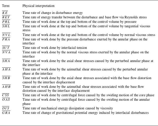
represent the control volume and surface area, respectively. The left-hand side of (2.54) represents the time rate of change in the disturbance energy within the control volume. The first term on the right-hand side of (2.54) represents the rate at which mechanical energy is transferred between the disturbance and base flow via Reynolds stress. The second and third terms correspond to the time rates of work conducted by pressure and viscous stress, respectively, whereas the fourth term represents the dissipation of mechanical energy because of viscosity. The fifth term represents the time rate of change in the gravitational potential energy induced by interfacial disturbances. Considering the normal and tangential dynamic boundary conditions at the interfaces, the energy budget model can be expressed as
 \begin{align} \overline{KE} &= \overline{REY} + \overline{PRL} + \overline{SHL} + \overline{NVL} + \overline{PRA} + \overline{SUT} + \overline{NVA}+ \overline{SHA} \notag \\ &\quad +\, \overline{AHA} + \overline{SHB} + \overline{AHB} + \overline{CSS} + \overline{OAS} + \overline{DIS}+\overline{GRA}. \end{align}
The specific expression for each term in (2.55) is given in Appendix C, the Clenshaw–Curtis quadrature is employed to evaluate the associated energy integrals. In (2.55) the first term
 $\overline{KE}$
on the left-hand side represents the time rate of change in disturbance energy. On the right-hand side, the term
 $\overline{REY}$
represents the time rate of energy transfer between the disturbance and base flow via Reynolds stress; the terms
 $\overline{PRL}$
,
 $\overline{SHL}$
and
 $\overline{NVL}$
represent the time rate of work done at the top and bottom of the control volume by pressure, tangential and normal viscous stress components, respectively. The selected control volume is periodic in the axial direction; therefore, the integral results of
 $\overline{PRL}$
,
 $\overline{SHL}$
and
 $\overline{NVL}$
are zero. Terms
 $\overline{PRA}$
,
 $\overline{SUT}$
and
 $\overline{NVA}$
represent the time rate of work attributed to the annular-phase pressure disturbance, time rate of work done by interfacial tension and time rate of work done by the normal viscous stress exerted by the annular phase on the interface. Terms
 $\overline{SHA}$
and
 $\overline{AHA}$
represent the time rate of work done by the axial and azimuthal shear stresses caused by the perturbed annular phase at the interface, respectively. Furthermore, terms
 $\overline{SHB}$
and
 $\overline{AHB}$
represent the time rate of work done by the axial and azimuthal shear stresses associated with the base flow distortion caused by the interface displacement, respectively; terms
 $\overline{CSS}$
and
 $\overline{OAS}$
represent the time rate of work done by centrifugal force caused by the swirling motion of the core and annular phases, respectively; the term
 $\overline{DIS}$
represents the time rate of mechanical energy dissipation caused by viscosity; and the term
 $\overline{GRA}$
represents the time rate of change of gravitational potential energy induced by interfacial disturbances. The physical meanings of the individual energy terms are summarised in table 2 of Appendix C.
The perturbation kinetic energy
 $\overline{EK}$
is employed to eliminate the non-uniqueness of each term in (2.55) because the eigenvector of the generalised eigenvalue problem (A3) is non-unique; that is, both sides of (2.55) are divided by
 $\overline{EK}$
to obtain
 \begin{align} {\textit{KE}}= \overline{KE}/\overline{EK},\quad \! REY = \overline{REY}/\overline{EK},\quad \! {\textit{PRL}} = \overline{PRL}/\overline{EK},\quad \!{\textit{SHL}} = \overline{SHL}/\overline{EK},\quad \! \text{etc.} \end{align}
The specific form of the perturbation kinetic energy
 $\overline{EK}$
is
 \begin{align} \overline{EK} = \frac {1}{2T\lambda } \int _0^T \int _0^\lambda \int _0^2 \int _0^1 \frac {\pi }{2} \big(\tilde {u}_1^2 + \tilde {v}_1^2 + \tilde {w}_1^2\big) r \, \textrm{d}r \, \textrm{d}\theta \, \textrm{d}z \, \textrm{d}t. \end{align}
Equation (2.56) is a commonly used expression for disturbance energy (Ding et al. Reference Ding, Mu, Si and Jian2022; Xu et al. Reference Xu, Mu, Xin, Qiao, Zhao and Si2024). A positive value for a certain term indicates that the energy promotes an interface disturbance, whereas a negative value indicates that the energy suppresses it.
3. Interfacial stability analysis
The interfacial stability of a spiral annular flow is affected by both the phase properties and velocity profiles; the mechanisms responsible for this instability are diverse. In the discussion on the influencing factors,
 ${\textit{Re}}$
can be adjusted by modifying
 $W^*_{max}$
. Here
 ${\textit{Re}}_{z}$
is altered by adjusting the axial velocity of the core phase in (2.39). We restrict both
 ${\textit{Re}}$
and
 ${\textit{Re}}_{z}$
to values below 1000, which is a commonly adopted range in linear stability analyses of a CAF (Hu & Joseph Reference Hu and Joseph1989; Orazzo et al. Reference Orazzo, Coppola and de Luca2014).
Variation in perturbation growth rate
 $\omega _i$
and frequency
 $\omega _r$
with axial wavenumber
 $k$
for different azimuthal modes at
 ${\textit{Oh}} = 0.047$
,
 $Re_z = 215$
,
 $V = 0.7$
,
 $N = 0.05$
,
 $J = 1.16$
and
 $R^{-1} = 0.5$
. The magenta dotted line in the disturbance frequency plots represents a reference line with a slope corresponding to the
 $V_1$
:
 $(a)\,m = 0,\,(b)\,m = 1, \,(c)\,m = 2, \,(d)\,m = 3, \,(e)\,m = 4$
and
 $(f)\,m = 5$
.

3.1. Influence of rotation on interfacial instability
First, we examine the effect of the circumferential velocity on the stability of the two-phase interface in a spiral annular flow because it is fundamental for sustaining the swirl. The analysis considers theoretical azimuthal modes from orders 0–5. Figure 3 illustrates the distributions of the disturbance growth rate and frequency versus the axial disturbance wavenumber for these modes. Since the disturbances grow exponentially in the form of
 ${\textrm e}^{\omega _it}$
, the maximum growth rate of the disturbance (denoted by
 $\omega _{\textit{i,max}}$
) dominates the instability of the two-phase swirling flow among all perturbations within the unstable region, and the corresponding axial wavenumber is
 $k_{max}$
(see figure 3
 $c$
). It should be noted that for each azimuthal mode, there exists a corresponding
 $\omega _{\textit{i,max}}$
and
 $k_{max}$
, and the azimuthal mode with the largest
 $\omega _{\textit{i,max}}$
governs the instability characteristics under the given flow conditions. As shown in figure 3, higher-order azimuthal modes (
 $m\geq 2$
) do not emerge across all rotational Reynolds numbers, and the instability in these modes arises only once the rotational Reynolds number exceeds a certain threshold. For example, at rotational Reynolds numbers of 10.8 and 21.5, only the
 $m = 0$
and
 $m = 1$
azimuthal modes are present, whereas no higher-order azimuthal modes (
 $m\geq 2$
) are observed. Within a small rotational Reynolds numbers range,
 $\omega _{\textit{i,max}}$
initially decreases and subsequently increases with an increase in
 ${\textit{Re}}$
. For example, in figures 3(
 $a$
) and 3(
 $b$
),
 $\omega _{\textit{i,max}}$
decreases markedly with an increase in
 ${\textit{Re}}$
from 10.8 to 21.5 before increasing significantly at
 $Re = 107.5$
. This behaviour reflects the dual role of the swirl in flow stability, which is in agreement with the findings of Xu et al. (Reference Xu, Mu, Xin, Qiao, Zhao and Si2024) concerning the instability of a rotating jet. At low rotational Reynolds numbers (e.g.
 $Re = 10.8$
and 21.5), the Froude number (
 $Fr$
) is very small, the dominant azimuthal mode of the flow instability is
 $m = 1$
, and flow is strongly influenced by gravity. At this stage, interfacial instability is most likely governed by a Rayleigh–Taylor instability (RTI). The interface remains unstable under disturbances of infinite wavelength because surface tension suppresses short-wavelength disturbances according to the RTI-type criterion. Consequently, the disturbance becomes stable only when the axial wavenumber exceeds a critical value, which is referred to as the cutoff axial wavenumber (
 $k_c$
). A cutoff axial wavenumber (
 $k_c$
) exists at any rotational Reynolds number. The disturbance growth rate becomes negative when the axial wavenumber exceeds
 $k_c$
; thus,
 $k_c$
defines the boundary of the unstable axial wavenumber range. The value of
 $k_c$
is related to the characteristic size of droplets formed by the rupture of the core phase. The cutoff axial wavenumber
 $k_c$
increases with an increase in the rotational Reynolds number, which results in a broader range of unstable axial wavenumbers. Meanwhile, the disturbance wavelength decreases (
 $\lambda = 2\pi /k$
). As the axial Reynolds number remains constant, the swirl number
 $S$
, which characterises the degree of swirl, increases with the rotational Reynolds number. Under such conditions, the Taylor vortex rings formed by interfacial bulging driven by circumferential rotation are more likely to break into smaller droplets.
For the stability analysis at an infinite wavelength (
 $k = 0$
), the flow remains stable under infinite-wavelength disturbances in the axisymmetric mode (
 $m = 0$
). In contrast, the spiral mode
 $m = 1$
can exhibit instability under such disturbances when the gravitational effects are significant; however, it becomes stable when gravity is weak. For the higher-order azimuthal modes (
 $m\geq 2$
), the instability at infinite wavelength occurs only when
 ${\textit{Re}}$
is sufficiently high. For example, at
 $Re = 107.5$
, the flow is stable in the
 $m = 3$
spiral mode; however, it becomes unstable at
 $Re = 215$
. Furthermore, the critical
 ${\textit{Re}}$
required for the onset of instability under infinite-wavelength disturbances increases with the azimuthal wavenumber. For example, the
 $m = 4$
spiral mode requires
 $Re = 215$
for instability to occur, whereas instability in the
 $m = 3$
spiral mode can be triggered at
 $Re = 107.5$
.
The real part
 $\omega _r$
of
 $\omega$
denotes the disturbance frequency and is plotted as a function of the axial wavenumber
 $k$
in figure 3. Within each azimuthal mode, the disturbance frequency increases approximately linearly with a constant gradient close to
 $V_1$
. This behaviour is reminiscent of the instability observed in rotating jets (Xu et al. Reference Xu, Mu, Xin, Qiao, Zhao and Si2024) and the standard temporal stability analysis of capillary jets (Eggers & Villermaux Reference Eggers and Villermaux2008). However, when
 $m=1$
, at certain rotational Reynolds numbers, for example,
 $Re=107.5$
and
 $215$
, and for all rotational Reynolds numbers in the higher-order helical modes
 $(m \geqslant 2)$
, the disturbance frequency exhibits a discontinuity, as highlighted by the purple circles in figure 3(b–f). This implies that disturbances propagate not only temporally but also axially in space, which resembles waves travelling within a fluid. Furthermore, to investigate the origin of the discontinuity in the disturbance growth rate and frequency (i.e. the emergence of a cusp), we carried out a diagnostic analysis of the eigenspectra, as presented in Appendix D. The results indicate that the cusp arises as a projection effect associated with branch switching between two eigenmode branches in the complex frequency plane.
(
 $a$
) Maximum disturbance growth rate
 $\omega _{\textit{i,max}}$
for different azimuthal modes as
 ${\textit{Re}}$
varies. (
 $b$
) Most unstable axial wavenumber
 $k_{max}$
for different azimuthal modes as
 ${\textit{Re}}$
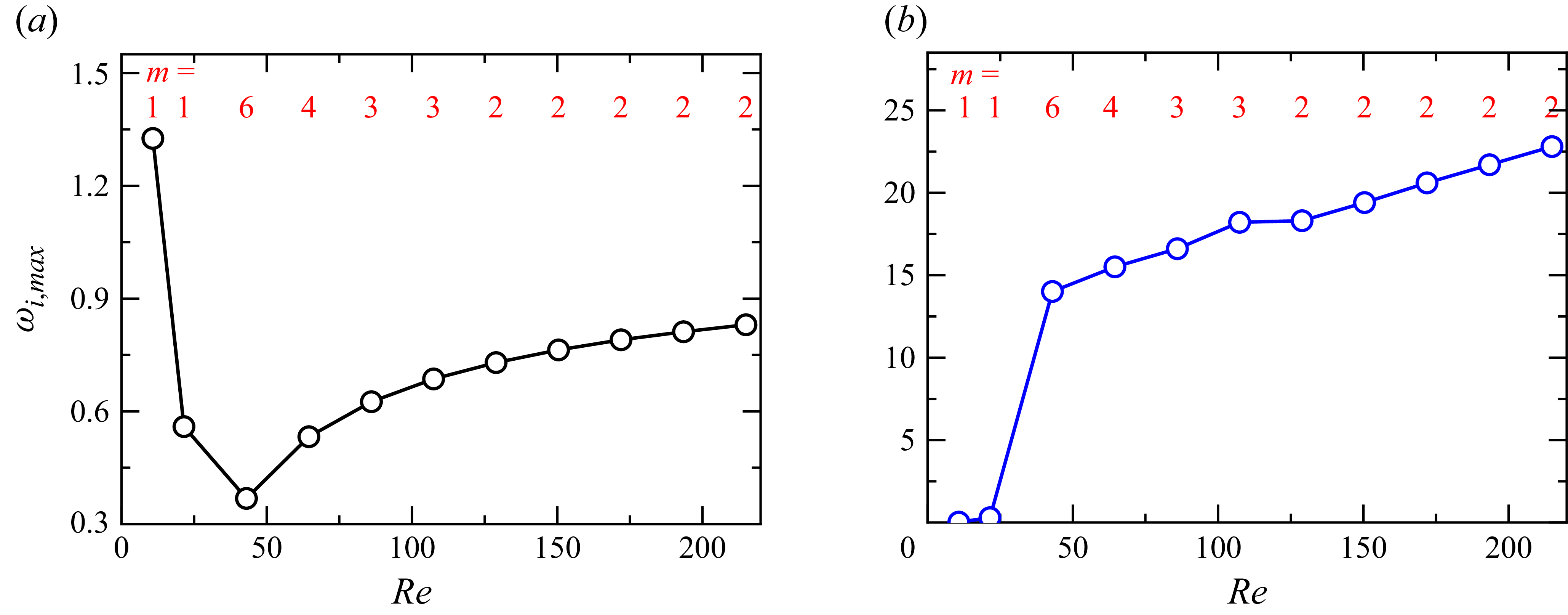
varies. The dominant azimuthal modes for each
 ${\textit{Re}}$
are highlighted in red font in the figures. The other flow parameters are identical to those used in figure 3.

Figure 4(
 $a$
) presents the maximum disturbance growth rates for the dominant azimuthal modes at various
 ${\textit{Re}}$
. As illustrated in figures 3(
 $a$
) and 3(
 $b$
), the maximum disturbance growth rate decreases initially and then increases with an increasing
 ${\textit{Re}}$
. This trend reflects the dual effect of rotational intensity on flow stability, and it corresponds to the different underlying instability mechanisms. At low
 ${\textit{Re}}$
,
 $Fr$
is small, which indicates a strong gravitational influence that leads to the RTI type. In this regime,
 $\omega _{\textit{i,max}}$
decreases sharply with increasing
 ${\textit{Re}}$
because the increasing rotational effect mitigates gravitational instability and promotes stabilisation. As
 ${\textit{Re}}$
continued to increase,
 $Fr$
increased accordingly, which diminishes the effect of gravity and leads to a shift in the dominant instability mechanism. Simultaneously, the dominant azimuthal mode varies with
 ${\textit{Re}}$
. In figures 4(a) and 4(b) the dominant azimuthal modes for each
 ${\textit{Re}}$
are marked in red. Once gravity ceases to be dominant, the azimuthal mode number increases rapidly with
 ${\textit{Re}}$
. In this process, the increase of
 ${\textit{Re}}$
acts to weaken the effect of gravity, and the rapid rise in the azimuthal mode number is determined by the axial velocity gradients of the two phases, which will be discussed in detail in § 3.2. As Re increases further, however, the occurrence of higher-order unstable azimuthal modes is suppressed. This behaviour contrasts with that observed in helical jet instabilities, where the azimuthal mode number increases with
 ${\textit{Re}}$
(Xu et al. Reference Xu, Mu, Xin, Qiao, Zhao and Si2024). Whether the unstable helical modes increase with
 ${\textit{Re}}$
in jets or decrease with
 ${\textit{Re}}$
in the present study, the underlying physical mechanism is the same: the strengthening centrifugal effect drives the lighter phase towards the core region (Zhang et al. Reference Zhang, He, Liu and Xu2022).
Figure 4(
 $b$
) illustrates the variation in the most unstable axial wavenumber
 $k_{max}$
with variations in
 ${\textit{Re}}$
. It can be seen that at very low rotational Reynolds numbers, for example,
 $Re=10.8$
and
 $Re=21.5$
, the dominant unstable azimuthal mode is
 $m=1$
, and the instability exhibits a long-wave character, with
 $k_{max}$
approaching zero. This occurs because
 $m=1$
corresponds to a global eccentric displacement of the entire core phase relative to the pipe centre. In the presence of a density contrast between the two phases, such displacement induces a first-order change in gravitational potential energy, which is amplified by buoyancy work, thereby giving rise to a long-wave instability. This mechanism weakens as the influence of gravity diminishes. Moreover, the emergence of such long-wave instability in density-stratified two-phase flows was already noted in the classical work of Yih (Reference Yih1967), who emphasised the long-wave instability induced by viscosity stratification, demonstrating that under low-inertia conditions, interfacial long waves can dominate the destabilisation. Hu & Joseph (Reference Hu and Joseph1989) extended this finding to a CAF, arguing that at extremely small viscosity ratios (
 $N \ll 1$
, such as in water–oil systems), the stability of a CAF can indeed be governed by long-wave disturbances (near the
 $k\to 0$
mode). As
 ${\textit{Re}}$
increases from 21.5 to 43, the corresponding
 $Fr$
also increases from 0.45 to 0.90, and the effect of gravity diminishes. At this stage, both
 $k_{max}$
and
 $m$
increase significantly. With further increases in
 ${\textit{Re}}$
, and hence, further weakening of the gravitational effects, the instability is driven by two-phase velocity gradients and circumferential rotation, which leads to a continued steady increase in
 $k_{max}$
.
Relative rate of change of energy with the axial wavenumber in different azimuthal modes at
 $Re = 107.5$
:
 $(a)\,m = 0, \,(b)\,m = 1, \,(c)\,m = 2, \,(d)\,m = 3, \,(e)\,m = 4$
and
 $(f)\,m = 5$
. The circle symbol in the figure represents the energy transfer corresponding to the maximum disturbance growth rate in each azimuthal mode; the other flow parameters are identical to those used in figure 3.

Figure 5 shows the energy budget results for the azimuthal modes of orders 0–5 and indicates the corresponding relative rate of change of energy at
 $k_{max}$
. The energy of some disturbances is very small (less than 1 % of the disturbance kinetic energy,
 ${\textit{KE}}$
) and is thus considered negligible for instability analysis; therefore, it is not shown in figure 5. Terms
 ${\textit{PRA}}$
,
 ${\textit{SHA}}$
,
 ${\textit{AHA}}$
and
 ${\textit{CSS}}$
have positive values, which indicate that these energy terms promote the development of disturbances. In contrast, terms
 ${\textit{SUT}}$
,
 ${\textit{OAS}}$
and
 ${\textit{DIS}}$
are negative, which implies the suppression of disturbance development. In this calculation,
 ${\textit{SHA}}$
consistently acts as the dominant contributor to instability, whereas
 ${\textit{DIS}}$
is the main suppressive term in the disturbance development. The contributions of
 ${\textit{SHA}}$
and
 ${\textit{DIS}}$
to the energy growth rate gradually increased with an increase in the azimuthal mode. Furthermore,
 ${\textit{AHA}}$
gradually surpasses
 ${\textit{PRA}}$
to become the second-largest contributor to the interface disturbance, which implies that the contribution of the circumferential shear energy term
 ${\textit{AHA}}$
becomes more prominent in higher-order spiral modes because the increased circumferential shear stress promotes the development of more azimuthal disturbance waves at the interface. This is consistent with the conclusion presented in Orazzo et al. (Reference Orazzo, Coppola and de Luca2014), which states that the annular shear mechanism is intrinsically linked to the development of spiral disturbances. The terms
 ${\textit{PRA}}$
,
 ${\textit{SHA}}$
and
 ${\textit{AHA}}$
are directly related to the KHI-type mechanism and
 $m = 3$
is the dominant azimuthal mode; the instability mechanism in this flow is classified as a KHI type. In this calculation, the interfacial tension energy term
 ${\textit{SUT}}$
suppresses the disturbance development; however, the term
 ${\textit{SUT}}$
does not always act as a suppressor in the swirl-induced instability of an immiscible/incompressible two-phase flow because its role is affected by
 ${\textit{Re}}$
,
 ${\textit{Re}}_{z}$
and
 $S$
. When
 ${\textit{SUT}}$
becomes positive, it behaves similarly to surface tension in capillary instability (CPI).
We analyse the energy budget of the dominant mode at the most unstable axial wavenumber with variations in
 ${\textit{Re}}$
, and figure 6 shows the variation in each energy term with variations in
 ${\textit{Re}}$
. At a low Reynolds number,
 ${\textit{GRA}}$
is the dominant energy term affecting interface instability and the instability mechanism is the RTI type. With increasing
 ${\textit{Re}}$
(e.g.
 $Re\geq 43$
),
 ${\textit{SHA}}$
becomes the dominant energy term that promotes the development of disturbances, suggesting that the instability mechanism at this point is of the KHI type. The term
 ${\textit{CSS}}$
became the dominant energy contribution from the interface disturbance with an increase in the rotational Reynolds number, which indicates a transition to the CTI-type mechanism (see figure 14). The rotating centrifugal energy term
 ${\textit{OAS}}$
of the annular phase plays an important role in suppressing disturbance development when the instability mechanism is of the CTI type. For example, at
 $Re = 21.5$
, the instability mechanism is of the CTI type, and the energy term
 ${\textit{OAS}}$
becomes the main stabilising term, which is different from the mechanism in the rotating jets instability, as the density of the surrounding air phase is considerably lower than that of the jet liquid in rotating jets, thereby resulting in
 ${\textit{OAS}}$
being very small. At a very low rotational Reynolds number (e.g.
 $Re = 10.8$
),
 ${\textit{GRA}}$
reaches the maximum value for all energy terms, which confirms that the instability mechanism is of the RTI type. Our research indicates that the dominant azimuthal mode is always
 $m = 1$
when the interface instability mechanism is of the RTI type. However, this azimuthal mode is not unique to RTI, and the azimuthal mode does not immediately shift to a higher-order mode when the instability mechanism transitions to another type. This is because the contribution of
 ${\textit{GRA}}$
to the disturbance kinetic energy
 ${\textit{KE}}$
remains significant. For example, in figure 6, at
 $Re = 21.5$
, the azimuthal mode remains as
 $m = 1$
although the instability mechanism is of the CTI type. In summary, the dominant energy term in the disturbance kinetic energy shifts from gravity and shear stress to the centrifugal force with an increase in
 ${\textit{Re}}$
, and the corresponding instability mechanism evolves accordingly.
Energy budget corresponding to the most unstable perturbation wave at the dominant azimuthal modes as
 ${\textit{Re}}$
varies under
 $Re_z = 215$
,
 $V = 0.7$
,
 ${\textit{Oh}} = 0.047$
,
 $N = 0.05$
,
 $J = 1.16$
and
 $R^{-1} = 0.5$
.

Variation of maximum disturbance growth rate
 $\omega _{\textit{i,max}}$
and most unstable axial wavenumber
 $k_{max}$
with
 ${\textit{Re}}_{z}$
at
 ${\textit{Oh}} = 0.047$
,
 $Re = 107.5$
,
 $N = 0.05$
,
 $J = 1.16$
and
 $R^{-1} = 0.5$
:
 $(a)\,V = 0.3, \,(b)\,V = 0.5, \,(c) \,V = 0.7, \,(d)\,V = 0.75$
. In each panel, the maximum disturbance growth rate corresponding to the dominant azimuthal mode is indicated by solid symbols and connected with a bold black line, while the most unstable axial wavenumber corresponding to the dominant azimuthal mode is marked by solid symbols and connected with a bold blue line. The most unstable azimuthal mode
 $m$
in each subfigure is highlighted in red.

3.2. Effect of axial motion on interfacial stability
The non-uniformity of the axial velocity distribution induces a pronounced velocity gradient, which in turn generates axial shear stress. The magnitudes of these forces are positively correlated with the velocity gradient and can significantly influence the stability of the interface. We investigate the effect of axial velocity magnitudes on interfacial stability in a two-phase spiral annular flow. Core and annular phases have distinct axial Reynolds numbers, and therefore, their stability characteristics are affected by
 $V_1$
and
 $V_2$
. Figure 7 shows the effect of proportional changes in
 $V_1$
and
 $V_2$
on stability. Proportional coefficients
 $V$
are set to 0.3, 0.5, 0.7 and 0.75, which correspond to the different flow states of the axial velocity shown in figure 2(
 $b$
). Figure 7 shows that the effect of
 $V$
on interfacial stability varies significantly with its magnitude. At a relatively low value of
 $V$
, such as
 $V = 0.3$
shown in figure 7(
 $a$
), the interfacial instability clearly exhibits non-monotonic behaviour; it first increases and then decreases with the rotational Reynolds number. Correspondingly, the most unstable axial wavenumber
 $k_{max}$
decreases sharply when
 $\omega _{\textit{i,max}}$
decreases; subsequently, its variation becomes more gradual. For
 $V = 0.5$
and
 $0.7$
, as shown in figures 7(
 $b$
) and 7(
 $c$
), increasing the rotational Reynolds number leads to a monotonic decrease in the maximum growth rate
 $\omega _{\textit{i,max}}$
of the interfacial disturbances. This implies that proportionally increasing the circumferential velocities of the two phases can enhance interfacial stability for these velocity ratios. However, their impacts on
 $k_{max}$
differ because of the differing numerical conditions: for
 $V = 0.5$
,
 $k_{max}$
decreases monotonically, whereas for
 $V = 0.7$
, it exhibits a generally increasing trend with fluctuations. Consequently, the sizes of the droplets formed by the breakdown of the Taylor vortex rings in
 $V$
values are different. For
 $V = 0.75$
shown in figure 7(
 $d$
), although the variation in
 $\omega _{\textit{i,max}}$
with increasing
 ${\textit{Re}}_{z}$
is less pronounced compared with the previously discussed cases (
 $V = 0.3, \,0.5$
and 0.7), it still shows a similar trend to that observed for
 $V = 0.3$
, where
 $\omega _{\textit{i,max}}$
first decreases and then increases. The variation in
 $k_{max}$
resembles that of
 $V = 0.7$
, thereby presenting an overall fluctuating upward trend. These findings suggest that
 ${\textit{Re}}_{z}$
has a dual effect on the interfacial instability of the two-phase flows. Increasing
 ${\textit{Re}}_{z}$
significantly reduces
 $\omega _{\textit{i,max}}$
when the axial velocities of the two phases maintain certain ratios (e.g.
 $V = 0.3$
, 0.5 and 0.7). This observation is consistent with the findings of Wereley & Lueptow (Reference Wereley and Lueptow1999) concerning single-phase Taylor–Couette–Poiseuille flow: a moderate axial flow stabilises the original centrifugal vortices, whereas a stronger axial flow re-induces instability beyond a new critical
 ${\textit{Re}}_{z}$
and axial wavenumber
 $k$
, which exhibits a dual effect on flow stability. Furthermore, increasing
 ${\textit{Re}}_{z}$
can lead to higher-order azimuthal modes becoming dominant in interfacial instability for
 $V$
values where azimuthal mode transitions occur (such as
 $V = 0.7$
and 0.75). In addition, higher
 $V$
values enable the emergence of higher azimuthal modes.
An energy budget analysis is conducted to clarify the mechanism by which the axial Reynolds number
 ${\textit{Re}}_{z}$
affects the stability of the two-phase interface. The results are presented in figure 8, where subfigures
 $(a), \,(b), \,(c)$
and
 $(d)$
correspond to cases with
 $V = 0.3, \,0.5, \,0.7$
and 0.75 in figures 7(a), 7(b), 7(c) and 7(d), respectively. In figure 8
 $(a)$
, for
 $V = 0.3$
, the dual effect of
 ${\textit{Re}}_{z}$
on
 $\omega _{\textit{i,max}}$
is reflected in the initial decreasing stage, during which the absolute magnitudes of both destabilising terms (
 ${\textit{PRA}}$
,
 ${\textit{SHA}}$
,
 ${\textit{AHA}}$
and
 ${\textit{CSS}}$
) and stabilising terms (
 ${\textit{SUT}}$
,
 ${\textit{OAS}}$
and
 ${\textit{DIS}}$
) decline, indicating a general tendency towards enhanced interfacial stability. A subsequent increase in
 $\omega _{\textit{i,max}}$
is attributed to an increase in
 ${\textit{PRA}}$
. Figure 8(
 $b$
) shows that the mechanism underlying the reduction in
 $\omega _{\textit{i,max}}$
is similar to that in figure 8(
 $a$
). All energy contributions diminish as
 ${\textit{Re}}_{z}$
increases; however, the decline in the destabilising terms is more pronounced than that in the stabilising terms, which results in a net reduction in the kinetic energy
 ${\textit{KE}}$
of the disturbance. In figures 8(
 $c$
) and 8(
 $d$
), azimuthal mode transitions occur, and the general trends of the energy terms are similar. However, in the case of
 $V = 0.75$
, term
 ${\textit{AHA}}$
exhibits a more substantial increase than that in
 $V = 0.7$
and surpasses
 ${\textit{PRA}}$
, which makes it the second-largest energy contributor to the interface disturbance. This finding aligns with the previously discussed spiral modal transformation (cf. figure 3). Compared with the higher-order azimuthal mode in figure 8(
 $d$
) with that in figure 8(
 $c$
), the rotation-induced energy contributions clearly enhance the instability mechanism.
Energy budget corresponding to the most unstable perturbation wave at the dominant azimuthal modes as
 ${\textit{Re}}_{z}$
varies: (
 $a$
)
 $V = 0.3$
, (
 $b$
)
 $V = 0.5$
, (
 $c$
)
 $V = 0.7$
and (
 $d$
)
 $V = 0.75$
. The other flow parameters are identical to those used in figure 7.

Effect of
 $V$
on the maximum disturbance growth rate
 $\omega _{\textit{i,max}}$
and azimuthal mode
 $m$
at
 ${\textit{Oh}} = 0.047$
,
 $Re = 107.5$
,
 $N = 0.05$
,
 $J = 1.16$
and
 $R^{-1} = 0.5$
: (
 $a$
)
 $V_1$
is fixed at three different values and
 $V_2$
is increased to vary
 $V$
, (
 $b$
)
 $V_2$
is fixed at three different values and
 $V_1$
is decreased to vary
 $V$
.

We analysed the effect of varying
 $V$
on the maximum growth rate of the interface disturbance
 $\omega _{\textit{i,max}}$
to investigate the effect of
 $V_1$
and
 $V_2$
on the interface stability in a non-uniform proportional state. In these calculations,
 $V$
was increased by either decreasing
 $V_1$
or increasing
 $V_2$
. Figure 9 shows the variation in
 $\omega _{\textit{i,max}}$
with
 $V$
for different
 $V_1$
values. Two distinct trends are observed: for smaller
 $V_1$
(e.g. 0.3),
 $\omega _{\textit{i,max}}$
increases monotonically with
 $V$
; however, this monotonic trend does not persist with an increase in
 $V_1$
. The swirl number
 $S = 1/V_1$
implies that the variation in
 $\omega _{\textit{i,max}}$
with
 $V$
is influenced by swirl intensity. Figure 9(
 $b$
) shows the variation in
 $\omega _{\textit{i,max}}$
with
 $V$
for three representative
 $V_2$
values. All cases exhibit a non-monotonic trend, first decreasing and then increasing. Differences between the three cases lie in the extent of the variation: a large
 $V_2$
results in a greater decrease, lower minimum
 $\omega _{\textit{i,max}}$
and more pronounced increase. As these
 $V_2$
values correspond to similar transformation scenarios, this supports the conclusion drawn from figure 9(
 $a$
) that changes in the swirl number
 $S$
modulate the pattern of
 $\omega _{\textit{i,max}}$
variation with
 $V$
.
As for the change in the azimuthal wavenumber
 $m$
with
 $V$
, both figures 9(
 $a$
) and 9(
 $b$
) indicate that the dominant azimuthal mode transitions from the axisymmetric mode (
 $m = 0$
) to spiral modes (
 $m\geq 1$
) when
 $V$
increases to a critical threshold (corresponding to the axial velocity of the two phases, which is non-monotonic). The higher-order spiral modes may become dominant when
 $V$
continues to increase. This observation is consistent with the analysis of Orazzo et al. (Reference Orazzo, Coppola and de Luca2014), who reported that increasing the axial Reynolds number of the annular phase in CAFs can shift the disturbance mode from axisymmetric to spiral. Our research indicates that the emergence of spiral modes is not attributed to an increase in the axial velocity (
 $V_2$
) of the annular phase; however, it is instead governed by the axial velocity ratio
 $V$
between the two phases. Increasing
 $V_2$
while keeping
 $V_1$
constant results in a higher
 $V$
, which leads to the onset of the spiral modes. Furthermore, as indicated by the analysis of the azimuthal wavenumber
 $m$
in figure 9, our findings reveal that a higher
 $V_2$
can induce higher-order spiral modes even when the value of
 $V$
remains unchanged.
Energy budget of the most unstable disturbance wave in the dominant mode varying with
 $V$
: (
 $a$
)
 $V_1 = 0.3$
, (
 $b$
)
 $V_1 = 0.5$
, (
 $c$
)
 $V_1 = 0.7$
, (
 $d$
)
 $V_2 = 0.3$
, (
 $e$
)
 $V_2 = 0.5$
and (
 $f$
)
 $V_2 = 0.7$
. The other flow parameters are identical to those used in figure 9. In each panel, the yellow region is marked as region I, characterised by the dominance of the
 ${\textit{PRA}}$
term in the instability energy. The grey region is marked as region II, where the instability is mainly governed by the
 ${\textit{SHA}}$
term. The blue region is marked as region III, which is characterised by a rapid growth of the
 ${\textit{AHA}}$
term that may even become the dominant contributor to the instability energy.

Figure 10 illustrates the effect of the axial velocity ratio
 $V$
on interface disturbances from the perspective of the energy budget. Subfigures (
 $(a$
), (
 $b$
) and (
 $c$
) correspond to
 $V_1 = 0.3$
, 0.5 and 0.7,respectively, while subfigures (
 $d$
), (
 $e$
) and (
 $f$
) correspond to
 $V_2 = 0.3$
, 0.5 and 0.7, respectively. For the monotonic increase in
 $\omega _{\textit{i,max}}$
with
 $V_1 = 0.3$
, a significant growth in
 $\omega _{\textit{i,max}}$
is observed before
 $V$
reaches 0.4 (see figure 9
 $a$
), which corresponds to region I in figure 10(
 $a$
). During this stage, the primary contributor to the interfacial disturbance energy (
 ${\textit{KE}}$
) is
 ${\textit{PRA}}$
, which increases gradually with
 $V$
. Once
 $V$
exceeds 0.4 and enters region II, the term
 ${\textit{SHA}}$
increases rapidly and becomes the dominant energy term driving instability. This corresponds to a sharp increase in
 $\omega _{\textit{i,max}}$
observed in figure 9(
 $a$
) for
 $V\approx 0.4\hbox{-}\hbox{-}0.6$
. The subsequent increase in
 $\omega _{\textit{i,max}}$
in region III is attributed to the growth of
 ${\textit{AHA}}$
, as shown in figure 10(
 $a$
). In figures 10(
 $b$
) and 10(
 $c$
), which correspond to
 $V_1 = 0.5$
and 0.7, respectively, region I is marked by a decreasing trend in
 ${\textit{PRA}}$
that persists over a wider range with an increase in
 $V_1$
. This explains the initial decline in
 $\omega _{\textit{i,max}}$
with an increase
 $V$
in figure 9(
 $a$
) for
 $V_1 = 0.5$
and 0.7. On entering region II, term
 ${\textit{SHA}}$
increases rapidly and overtakes
 ${\textit{PRA}}$
as the dominant contributor to the disturbance energy term. In region III, a further increase in
 $V$
leads to a decrease in
 ${\textit{SHA}}$
and a continuous increase in
 ${\textit{AHA}}$
, which eventually surpasses
 ${\textit{SHA}}$
and becomes the leading disturbance energy term. This transition corresponds to the onset of the azimuthal mode transformation (see figure 9
 $a$
), where the dominant mode shifts from the axisymmetric mode (
 $m = 0$
) to the spiral mode (
 $m\geq 1$
), analysed previously, the circumferential shear energy term (
 ${\textit{AHA}}$
) contribution becomes more pronounced under higher-order azimuthal modes. Similar mechanisms can be observed in figures 10(
 $d$
), 10(
 $e$
) and 10(
 $f$
). In region I the term
 ${\textit{PRA}}$
dominates and decreases with an increase in
 $V$
, which leads to a decrease in
 $\omega _{\textit{i,max}}$
in figure 10(
 $b$
). In region II,
 ${\textit{SHA}}$
increases rapidly, overtaking
 ${\textit{PRA}}$
. In region III the term
 ${\textit{SHA}}$
tends to decline, whereas the term
 ${\textit{AHA}}$
continues to increase and may even replace
 ${\textit{SHA}}$
as the dominant disturbance energy term. This highlights the significant role of the rotational energy term in higher-order azimuthal modes. The effect of the axial velocity ratio
 $V$
on interfacial instability can be attributed to the dynamic competition among the energy terms
 ${\textit{PRA}}$
,
 ${\textit{SHA}}$
and
 ${\textit{AHA}}$
. This process effectively reshapes the optimal disturbance structure under different flow rate ratios, which is consistent with the findings of Orazzo et al. (Reference Orazzo, Coppola and de Luca2014) on disturbance evolution. As
 $V$
increased, the dominant energy term transitioned from
 ${\textit{PRA}}$
and
 ${\textit{SHA}}$
to
 ${\textit{AHA}}$
, which reflects the increasing impact of the rotational effects associated with higher-order azimuthal modes.
3.3. Effect of core-phase proportion on interfacial stability
The volume fraction of the core phase significantly influences the axial velocity distribution (see figure 2
 $c$
) and affects the azimuthal velocity, because the latter depends solely on the radial positions of the two phases ((2.37) and (2.38)). Therefore, we investigated the effect of the core-phase volume ratio on flow stability in detail. Different volume fractions of the core phase can be represented by varying parameter
 $R^{-1}$
. Without loss of generality, we explore the range
 $R^{-1}$
= 0.3–0.7 and present the resulting stability characteristics in figure 11. The effect of the core-phase volume fraction on interfacial stability is complex and exhibits strong coupling with swirl intensity, as shown in figure 11(
 $a$
–
 $e$
), for varying
 $V$
from 0.3 to 0.7. From the results shown in figures 11(
 $a$
) and 11(
 $b$
),
 $\omega _{\textit{i,max}}$
increases rapidly with an increasing
 $R^{-1}$
. The enhanced Poiseuille component introduced by the axial flow played a significant destabilising role. At low swirl numbers (e.g.
 $S = 0.5$
), the Poiseuille contribution is more substantial, which leads to a greater variation in
 $\omega _{\textit{i,max}}$
. At higher axial velocity ratios, such as
 $V = 0.6$
and 0.7,
 $\omega _{\textit{i,max}}$
initially increases with
 $R^{-1}$
, reaches a peak and subsequently decreases. This behaviour is consistent with the concept of ‘the most unstable gap width’, wherein excessively narrow gaps suppress the growth of azimuthal modes because of boundary layer induced dissipation (Lathrop, Fineberg & Swinney Reference Lathrop, Fineberg and Swinney1992). This mechanism is further supported by the evolution of the azimuthal wavenumber
 $m$
, as shown in figure 11(
 $f$
). As
 $R^{-1}$
increases, the dominant mode transitions from higher azimuthal wavenumbers to axisymmetric modes (
 $m = 0$
); this aligns with observations in the Taylor–Couette flow, where reducing the gap between the inner and outer walls promotes the emergence of vortex structures with low azimuthal wavenumbers (Razzak, Khoo & Lua Reference Razzak, Khoo and Lua2019). Furthermore, the presence of axial flow introduces a Poiseuille component into an otherwise purely rotational flow. This not only changes the overall level of instability but also shifts the optimal geometric configuration for instability, which changes the peak growth rate position (Graham Reference Graham1998), as clearly observed in figure 11(
 $c$
–
 $e$
).
Effect of
 $R^{-1}$
on the maximum disturbance growth rate
 $\omega _{\textit{i,max}}$
and azimuthal mode
 $m$
at
 $Re = 107.5$
,
 $N = 0.05$
and
 $J = 1.16$
: (
 $a$
)
 $V = 0.3$
, (
 $b$
)
 $V = 0.4$
, (
 $c$
)
 $V = 0.5$
, (
 $d$
)
 $V = 0.6$
, (
 $e$
)
 $V = 0.7$
, (
 $f$
) azimuthal mode varies with
 $R^{-1}$
at
 $V = 0.7$
. Each subfigure includes three swirl number pairs,
 $S = 0.5$
, 1.0 and 1.5.

Energy budget of the most unstable disturbance wave in the dominant mode varying with
 $R^{-1}$
: (
 $a$
)
 $V = 0.3$
, (
 $b$
)
 $V = 0.4$
, (
 $c$
)
 $V = 0.5$
, (
 $d$
)
 $V = 0.36$
and (
 $e$
)
 $V = 0.7$
. The other flow parameters are identical to those used in figure 11.

Figure 12 shows the variation in the energy budget corresponding to the stability results in figure 11. Subfigures (
 $a$
)–(
 $e$
) of figure 12 correspond to the same values of
 $V$
as in figure 11(
 $a$
–
 $e$
), respectively. In figures 12(
 $a$
) and 12(
 $b$
), the sharp increase in
 $\omega _{\textit{i,max}}$
observed in figures 11(
 $a$
) and 11(
 $b$
) is primarily driven by the rapid rise in the term
 ${\textit{PRA}}$
where the swirl number is
 $S = 0.5$
. This aligns with our earlier analysis that the axial velocity introduces a significant Poiseuille component at low swirl intensities. This enhances the contribution of the annular-phase pressure disturbances to interfacial instability, continuously supplying energy to the disturbance at the interface. In addition, energy terms associated with the swirling motion, specifically
 ${\textit{CSS}}$
and
 ${\textit{OAS}}$
, significantly contribute to the kinetic energy of the interface disturbance
 ${\textit{KE}}$
. At higher swirl numbers (e.g. figure 12
 $a$
,
 $S = 1.5$
), the OAS term surpasses the dissipation term (
 ${\textit{DIS}}$
) to become the dominant stabilising energy term, indicating the centrifugal stability mechanism of the annular phase. The energy term variation shown in figure 12(
 $c$
) represents a transitional regime in which the dominant contribution to the disturbance kinetic energy shifts from
 ${\textit{PRA}}$
to
 ${\textit{SHA}}$
. In subsequent cases, as shown in figures 12(
 $d$
) and 12(
 $e$
), the term
 ${\textit{SHA}}$
consistently dominates disturbance energy terms of the interface disturbance. Although figures 11(
 $d$
) and 11(
 $e$
) both show a decreasing trend in
 $\omega _{\textit{i,max}}$
with increasing
 $R^{-1}$
, the underlying mechanisms differ significantly, as indicated in figures 12(
 $d$
) and 12(
 $e$
). In figure 12(
 $d$
) the reduction in
 $\omega _{\textit{i,max}}$
results from a balance between the Poiseuille component of the axial velocity and the velocity gradient induced by circumferential rotation, which reflects a comprehensive change between the energy production and dissipation terms. In contrast, in figure 12(
 $e$
) the decrease in
 $\omega _{\textit{i,max}}$
is more closely associated with the mechanism described by the ‘most unstable gap width’ concept. As
 $R^{-1}$
continues to increase, the viscous dissipation term
 ${\textit{DIS}}$
increases steadily and becomes the primary factor that limits the growth of interfacial disturbances.
Effects of fluid property parameters on flow stability:
 $(a)$
influence of the viscosity ratio
 $N$
on the disturbance growth rate;
 $(b)$
dominant energy contributions associated with the two peaks in the
 $\omega _i-k$
curve at
 $N=0.05$
;
 $(c)$
dominant energy contributions associated with the two peaks in the
 $\omega _i-k$
curve at
 $N=0.1$
;
 $(d)$
influence of the density ratio
 $J$
on the disturbance growth rate, together with the dominant energy contributions corresponding to the two peaks in the
 $\omega _i-k$
curve at
 $J=1$
. The most unstable azimuthal mode
 $m$
in each case is highlighted in red, and the other flow parameters are
 $Re=105, \,Re_z=215, \,Fr=2.26, \,R^{-1}=0.5, \,V=0.5$
, with
 $J=1.16$
in (a–c) and
 $N=0.05$
in
 $(d)$
.

3.4. Effect of fluid physical parameters on interfacial stability
We conducted a detailed investigation into the influence of the physical properties of the working fluids on flow stability, with particular emphasis on the effects of the viscosity ratio and density ratio on the disturbance growth rate and disturbance modes. The influence of the viscosity ratio
 $N$
is shown in figure 13
 $(a)$
. Here, the two-phase average axial velocity ratio is fixed at
 $V=0.5$
, such that the dominant unstable mode is the axisymmetric mode with azimuthal wavenumber
 $m=0$
. As
 $N$
increases, the variation of
 $\omega _{\textit{i,max}}$
is not monotonic. Specifically,
 $\omega _{\textit{i,max}}$
increases as
 $N$
rises from 0.005 to 0.01, decreases as
 $N$
increases further from 0.01 to 0.1 and then grows again as
 $N$
increases from 0.1 to 1. Notably, when
 $N=0.05\,\text{and}\,0.1$
, the
 $\omega _{i}-k$
curves exhibit two distinct peaks, denoted as
 $P_1$
and
 $P_2$
, suggesting the coexistence of different instability mechanisms. To clarify this, the variation of
 $\omega _{i}$
and the corresponding energy budgets with respect to
 $k$
for
 $N=0.05\,\text{and}\,0.1$
are presented in figures 13
 $(b)$
and 13
 $(c)$
, respectively. Since our aim is to identify the dominant instability mechanisms, only the leading destabilising and stabilising energy terms are shown. It is observed that
 $P_1$
is primarily driven by the
 ${\textit{CSS}}$
term and suppressed by the
 ${\textit{OAS}}$
term, whereas
 $P_2$
is driven by the
 ${\textit{PRA}}$
term and suppressed by the
 ${\textit{DIS}}$
term. Accordingly,
 $P_1$
corresponds to the CTI mechanism, whereas
 $P_2$
corresponds to a Kelvin–Helmholtz-type instability mechanism.
The effect of the density ratio
 $J$
is illustrated in figure 13
 $(d)$
. When
 $J\lt 1$
, centrifugal forces can promote the appearance of spiral unstable modes even at
 $V=0.5$
. This instability mechanism resembles the helical instability observed in a liquid jet surrounded by air (Xu et al. Reference Xu, Mu, Xin, Qiao, Zhao and Si2024). Furthermore, for
 $J=1$
, the
 $\omega _{i}-k$
curves also exhibit two peaks,
 $P_1$
and
 $P_2$
. The corresponding energy budget analysis again confirms that
 $P_1$
arises from the CTI mechanism, whereas
 $P_2$
corresponds to the Kelvin–Helmholtz-type instability mechanism.
4. Transformation of interface instability mechanisms
In our study, interfacial stability is governed by the combined action of gravitational, capillary, axial and azimuthal shear, and centrifugal forces. Furthermore, our results indicate that the RTI is always associated with a dominant spiral mode
 $m = 1$
, which indicates a clear linkage between the type of instability mechanism and transformation of the dominant azimuthal mode. Therefore, this section presents a detailed discussion of transformation mechanisms underlying different instability types. We consider four types of instability mechanisms, each corresponding to specific energy terms in the energy budget. The term
 ${\textit{GRA}}$
associated with gravity corresponds to the RTI type. The term
 ${\textit{SUT}}$
, related to interfacial tension, represents CPI. Although
 ${\textit{SUT}}$
suppresses the development of interfacial disturbances, the term
 ${\textit{SUT}}$
is not always negative. Under certain conditions, it can become positive and even serve as the dominant energy source driving instability. The terms
 ${\textit{PRA}}$
,
 ${\textit{SHA}}$
and
 ${\textit{AHA}}$
associated with pressure disturbances and axial and circumferential shear in the annular phase correspond to a KHI. The term
 ${\textit{CSS}}$
, which is induced by circumferential rotation, corresponds to a CTI. In analysing these mechanisms, we consider the effect of parameters such as
 ${\textit{Re}}$
,
 ${\textit{Re}}_{z}$
,
 $V$
and
 $R^{-1}$
because each of these factors correspond to key influencing parameters discussed in § 3.
Phase diagrams of the dominant interfacial instability mechanisms in the
 $Re_z-Re$
space at
 $J=1.16$
and
 $N = 0.05$
:
 $(a)$
 $R = 0.3, \,V=0.5; \,(b)\,R= 0.5, \,V = 0.5; \,(c)\,R = 0.7, \,V = 0.5; \,\text{and}\,(d)\,R=0.5, \,V=0.7$
. In each panel, RTI, CPI, KHI and CTI types are indicated by black circles, orange diamonds, red squares and green triangles, respectively.

Figure 14 presents a phase diagram of instability mechanisms within the
 $Re-Re_z$
space. Figures 14(
 $a$
), 14(
 $b$
) and 14(
 $c$
) correspond to nearly identical flow conditions, with the only variation being the core-phase volume fraction, i.e.
 $R^{-1} = 0.3$
, 0.5 and 0.7, respectively. The distribution of the instability mechanisms at the interface changes significantly with an increase in
 $R^{-1}$
from 0.3 to 0.7. The annular-phase thickness is large when the core radius is small (e.g.
 $R^{-1} = 0.3$
), and the CTI type dominates the entire moderate-to-high rotational Reynolds number regime. The KHI type appears only within a moderate
 ${\textit{Re}}$
range, and its domain shrinks with increasing
 ${\textit{Re}}_{z}$
. This observation is consistent with the findings of Picardo, Garg & Pushpavanam (Reference Picardo, Garg and Pushpavanam2015) who demonstrated that CTIs are more likely to occur when the annular phase occupies a larger volume fraction. Furthermore, our analysis reveals that a distinct instability mechanism classified as the CPI type emerges at low core-phase volume fractions. This mechanism indicates a low axial and azimuthal interfacial shear, which explains the difficulty in triggering the KHI type under these conditions. As shown in figure 14(
 $b$
), the threshold
 ${\textit{Re}}$
required to trigger the CTI type increases with an increase in
 $R^{-1}$
. Concurrently, the interfacial shear stress and pressure disturbance of the annular phase becomes more prominent, making the KHI type more likely. To some extent, a trend consistently observed in figures 14(
 $a$
), 14(
 $b$
) and 14(
 $c$
) is that increasing
 ${\textit{Re}}_{z}$
can reactivate the CTI type. In fact, the transition from the KHI type to the CTI type with increasing
 ${\textit{Re}}_{z}$
is governed by the contribution of the pressure-related energy term
 ${\textit{PRA}}$
. Although
 ${\textit{PRA}}$
is often associated with the KHI-type instability, it reflects pressure perturbations in the annular phase acting on the interface, and therefore, it is not exclusively indicative of the KHI type. An alternating pattern between the CTI- and KHI-type mechanisms is observed at low
 ${\textit{Re}}$
across all three subfigures, which corresponds to the energy budget trends shown in figure 6. Under stronger shear conditions, increasing
 ${\textit{Re}}_{z}$
eventually leads to a dominance of the KHI creep mechanism as illustrated in figures 14(
 $b$
) and 14(
 $c$
). This transition results from the elevated axial shear stress, which substantially increases the
 ${\textit{SHA}}$
term. A KHI-type mechanism is triggered once
 ${\textit{SHA}}$
becomes the leading contributor to the disturbance energy. This conclusion is further supported by the findings of Picardo et al. (Reference Picardo, Garg and Pushpavanam2015), who demonstrated that the CTI tends to occur at lower
 ${\textit{Re}}$
, whereas axial shear-driven instabilities (KHI) prevail at higher
 ${\textit{Re}}$
.
Computational conditions for figure 14(
 $d$
) are essentially the same as those for figure 14(
 $b$
), with the only significant difference being
 $V$
;
 $V = 0.5$
in figure 14(
 $b$
), while figure 14(
 $d$
) corresponds to
 $V = 0.7$
. This implies that the case presented in figure 14(
 $d$
) involves a stronger interfacial shear, as inferred from (2.50) and (2.51). Similarly, we observe the emergence of a CTI-type mechanism at low
 ${\textit{Re}}$
in figure 14(
 $d$
), which is consistent with previous findings. In addition, across all panels in figure 14, we observe the occurrence of the RTI-type mechanism at extremely low
 ${\textit{Re}}$
values. Figure 14(
 $c$
) illustrates that the axial shear intensifies with an increase in
 ${\textit{Re}}_{z}$
, which diminishes the effect of the RTI-type mechanism. Then, the instability exhibits characteristics that are more typical of a KHI-type growth behaviour, indicating a transition in the dominant instability mode.
5. Conclusion and outlook
A three-dimensional linear temporal stability analysis method was employed to analyse the interfacial instability of a spiral CAF, and the influence of gravity on the interfacial stability of separated two-phase fluids was examined. The following conclusions were obtained from this study. We found that gravity played a dominant role when
 ${\textit{Re}}$
was very small because the Froude number was very small at this stage. The
 $m = 1$
spiral mode was the unstable azimuthal mode governed by gravity. The variations in
 ${\textit{Re}}$
exerted a dual effect on the instability of the two-phase interface in the axisymmetric mode. Higher-order spiral modes (
 $m\geq 2$
) emerged only when
 ${\textit{Re}}$
exceeded a certain threshold, and the dominant azimuthal mode number decreased with increasing
 ${\textit{Re}}$
because of the density difference between the two phases and effect of centrifugal force. This behaviour is observed only when the density ratio
 $J\gt 1$
. In contrast, when
 $J\lt 1$
, the dominant azimuthal mode number increases with increasing
 ${\textit{Re}}$
. The analysis of interfacial instability under infinitely long disturbance waves suggested that the interface was stable in the axisymmetric mode. For the spiral mode with
 $m = 1$
, the stability was strongly affected by gravity. The interface became unstable when gravitational effects were significant because the surface tension tended to suppress short-wave disturbances. The interface remained stable under weak gravity. For higher-order spiral modes with
 $m\geq 2$
, the instability was closely associated with the Reynolds number. Each spiral mode possessed a critical threshold
 ${\textit{Re}}$
above which the interface became unstable under infinitely long disturbance waves. Furthermore, this critical threshold increased with the azimuthal mode number.
The results of the energy budget analysis revealed that circumferential shear energy was intimately linked to the emergence of higher-order spiral modes. The effect of circumferential shear stress increased with an increase in the azimuthal mode number. Although the effect of
 ${\textit{Re}}_{z}$
on interfacial instability exhibited a dual nature, it promoted the emergence of higher-order azimuthal modes. In addition, the emergence of the spiral modes was governed by the value of
 $V$
, which needs to be sufficiently large to induce a non-monotonic axial velocity profile between phases. The effects of
 ${\textit{Re}}_{z}$
and
 $V$
on the interfacial instability were attributed to the dynamic interplay between the terms
 ${\textit{PRA}}$
,
 ${\textit{SHA}}$
and
 ${\textit{AHA}}$
. The effect of the ratio of core to annular phase on interfacial instability was investigated, and the notion of ‘the most unstable gap width’ is considered here, wherein instability was maximised. In addition, the viscous dissipation in the system increased with an increase in the proportion of the core phase, suppressing the development of higher-order azimuthal modes. Finally, based on the results of the energy budget analysis, a phase diagram of the instability mechanisms in the
 $Re_z-Re$
space was presented. Four types of instability mechanisms, i.e. RTI, CPI, KHI and CTI, were systematically examined considering the effects of
 $V$
and
 $R^{-1}$
. This study is expected to offer valuable insights into the physical mechanisms governing the instability of incompressible and immiscible two-phase spiral CAFs in confined domains and can inform applications such as oil–water cyclone separation, efficient multiphase transport and accurate multiphase flow metering.
At the end of this paper, we outline future research directions concerning an incompressible two-phase swirling CAF. These will primarily focus on global stability characteristics and the rheological behaviour of non-Newtonian fluids. We note that the dominant modes and their associated disturbance frequencies identified by the linear analysis do not vanish in the nonlinear flow field; rather, they transform into the prevailing coherent structures, which govern the energy transfer and dynamical evolution through strong triadic resonant interactions (Schmidt & Oberleithner Reference Schmidt and Oberleithner2023). Therefore, an important direction for future research is to investigate the correlation between the most unstable modal growth rates and frequencies predicted by linear stability analysis and the interfacial instabilities observed in nonlinear numerical simulations and experiments of density- and viscosity-stratified flows. In this study we also performed nonlinear numerical simulations to gain a more intuitive understanding of the interfacial instability in an immiscible two-phase flow. The corresponding results are presented in Appendix E. Another important research avenue concerns the influence of the non-Newtonian rheological properties of the core phase on interfacial stability, as it is typically a highly viscous non-Newtonian fluid (e.g. oil) in practical industrial applications.
Acknowledgements
The authors gratefully acknowledge the anonymous reviewers for their insightful and constructive comments, which have greatly helped to improve the quality of this paper.
Funding
This work was supported by the Youth Innovation Promotion Association of Chinese Academy of Sciences (Grant No. 292023000133) and the National Natural Science Foundation of China (Grant No. 11972039).
Declaration of interests
The authors report no conflict of interest.
Author contributions
Jian Zhang derived the theory and Hu Chen performed the calculation. All authors contributed equally to analysing data and reaching conclusions, and in writing the paper.
Appendix A. Numerical solution procedure and verification
The Chebyshev collocation method is a high-precision numerical technique based on Chebyshev polynomials. The fundamental principle is discretising continuous problems into algebraic equations by selecting specific collocation points (Chebyshev nodes) and exploiting the orthogonality and convergence advantages of Chebyshev polynomials to obtain efficient solutions. When solving the interfacial stability of a two-phase flow, the actual domain of the core phase
 $r\in [0,1]$
is mapped onto the computational domain
 $y\in [-1,1]$
through a linear transformation
 \begin{align} r = \frac {1 + y}{2}. \end{align}
Likewise, the actual domain
 $r\in [1,R]$
of the annular phase is mapped onto the computational domain
 $y\in [-1,1]$
using another linear transformation:
 \begin{align} r = \frac {y(R - 1) + (R + 1)}{2}. \end{align}
The perturbed physical quantities
 $\hat {u}_i$
,
 $\hat {v}_i$
,
 $\hat {w}_i$
,
 $\hat {p}_i$
and
 $\hat {\eta }$
together with their derivatives are expanded in terms of Chebyshev polynomials and substituted into the perturbed governing equations to yield discrete algebraic equations. The Chebyshev–Gauss–Lobatto nodes
 $y_j = \cos ( j\pi / N ))$
and
 $j = 0, 1, \ldots , N$
are employed for discretising the computational domain. This can effectively suppress the Runge phenomenon because the nodes are more densely distributed near both ends of the interval. Therefore, the algebraic equations formed by discretising the disturbance-governing equations and corresponding boundary conditions become a generalised eigenvalue problem of the form
 \begin{align} [\boldsymbol{A}]\boldsymbol{X} = \textrm{i}\omega [\boldsymbol{B}]\boldsymbol{X}, \end{align}
where
 $\boldsymbol{X}$
represents a characteristic vector. According to the construction of Chebyshev–Gauss–Lobatto nodes, the number of nodes for the annular and core phases are
 $N_1 + 1$
and
 $N_2 + 1$
, respectively. Therefore, the sizes of the matrices
 $\boldsymbol{A}$
and
 $\boldsymbol{B}$
are both (
 $4N_1 + 4N_2 + 9$
)
 $\times$
 $(4N_1 + 4N_2 + 9)$
. A MATLAB code is developed to solve the generalised eigenvalue problem using the QZ algorithm, where
 $\boldsymbol{B}$
is a singular matrix. At this stage, we complete the construction of the Chebyshev collocation method.
The number of collocation points
 $N$
significantly affects the accuracy of the solution when employing the Chebyshev collocation method. Therefore, different values are initially assigned to
 $N_1$
and
 $N_2$
to solve
 $\omega$
 $\omega = \omega _r+\textrm{i}\omega _i$
for verifying the suitability of the selected values of
 $N$
. A smaller value of
 $N_1$
is sufficient to capture the detailed results because the axial velocity in the core layer is relatively smooth without sharp variations (see figure 2). In contrast, a higher value of
 $N_2$
is required because of the steep velocity gradient in the annular layer. We tested the values of
 $N_1$
and
 $N_2$
at
 $R^{-1} = 0.5$
, and the results are presented in table 1. There is only a slight difference in the calculated results when
 $N_1\geq 20$
and
 $N_2\geq 70$
, and therefore, the collocation point configurations of
 $N_1 = 30$
and
 $N_2 = 80$
are adopted.
Calculated complex frequency
 $\omega (=\omega _r+\textrm{i}\omega _i)$
under different values of
 $N_1$
and
 $N_2$
, where
 $R^{-1} = 0.5, \,Re = 215, \,Re_{z} = 215, \,We = 102.4, \,V = 0.5, \,J = 1.16, \,N = 0.05, \,m = 0 \ {\textrm and} \,k = 5$
.

Three benchmark strategies are employed to verify the accuracy of the proposed method. In figure 15(
 $a$
) the annular-phase fluid is not considered (i.e.
 $J = N = 0$
) and the basic flow state of the core-phase fluid comprises solely of circumferential motion (i.e.
 $V_1 = V_2 = 0$
). In this case, the calculation aligns with the model proposed by Kubitschek & Weidman (Reference Kubitschek and Weidman2007). Setting
 $m = 3$
, the calculated results are compared with those of Kubitschek & Weidman (Reference Kubitschek and Weidman2007) and show good agreement. In figure 15
 $(b)$
the liquid exhibits a spiral jet motion in a gaseous environment, with both fluids exhibiting axial and circumferential motions. The circumferential velocity is described by a Rankine vortex, whereas the axial velocity of the liquid is expressed in the same manner as in this study. The axial motion of the gas is analysed using the error function derived by Xu et al. (Reference Xu, Mu, Xin, Qiao, Zhao and Si2024), which can be expressed as (A4).
We compared the results obtained using the computational approach adopted in this study with those of Xu et al. (Reference Xu, Mu, Xin, Qiao, Zhao and Si2024) by setting
 $m = 0$
. The comparison revealed an excellent agreement, validating the accuracy and reliability of the proposed method. In summary, our numerical methodology and its implementation demonstrate satisfactory consistency in the stability analysis of both the swirling core flow and the immiscible two-phase swirling flow with axial shear. Therefore, the Chebyshev spectral method employed in this study is suitable to address the problem of interfacial disturbance development, and the constructed solution code is confirmed to be correct.
 \begin{align} U_2(r) = V \left [ (W - V_S) \text{erf} \left ( \frac {\sqrt {\pi }}{2} \frac {4(V_S - 1)}{N(W - V_S)} (r - 1) \right ) + V_S \right ] \quad \text{at} \quad r \gt 1. \end{align}
Verification of the accuracy of the numerical solution code.
 $(a)$
Liquid column swirl in a vacuum, where
 $Re = 10$
,
 $We = 100$
,
 $J = 0$
,
 $N = 0$
,
 $V_1 = 0$
,
 $V_2 = 0$
and
 $m = 3$
. The calculation results of the present study are compared with those of Kubitschek & Weidman (Reference Kubitschek and Weidman2007).
 $(b)$
Jet of the rotating liquid in a gaseous environment; the axial velocity of the gas follows an error function (A4), where
 $Re = 20.5$
,
 $We = 71.3$
,
 $V = 3.5$
,
 $V_S = 0.995$
,
 $W = 0$
,
 $J = 0.0013$
,
 $N = 1.67\times 10^{-4}$
and
 $m = 0$
. The comparison is between the results calculated using this method and those obtained by Xu et al. (Reference Xu, Mu, Xin, Qiao, Zhao and Si2024).

Appendix B. Derivation of the axial velocity of two-phase spiral annular flow
The core and annular phases are assumed to be perfectly axisymmetric, with the fully developed flow being a function solely of the radial coordinate, represented by
 $\boldsymbol{U^*_i}(\boldsymbol{r})=U^*_i(r) \boldsymbol{e_z}+W^*_i(r) \boldsymbol{e_{\theta }}$
, where
 $i=1$
and 2, which represent the core and ring phases, respectively. From (2.2), we obtain
 \begin{align} \frac {1}{r} \frac {d}{{\textrm d}r} \left ( r \frac {{\textrm d} U_i^*}{{\textrm d}r} \right ) = \frac {1}{\mu _i} \frac {\partial p_i^*}{\partial z}. \end{align}
The general solution to (B1) is
 \begin{align} U_i^* = \frac {1}{4 \mu _i} \frac {\partial p_i^*}{\partial z} r^2 + C_1^* \ln r + C_2^*. \end{align}
For the core phase, the boundary condition
 $r = 0$
is
 \begin{align} C_2^* = U_S^* - \frac {r_1^2}{4 \mu _1} \frac {\partial p_1^*}{\partial z}. \end{align}
Here
 $U_1^*$
is a finite value, and therefore, the constant
 $C_1^*$
must be zero. At the two intersecting interfaces (
 $r = r_1$
), the velocity is assumed to be
 $U_S$
. The pressure drop
 ${\partial p_i^*}/{\partial z}$
can be expressed as
 \begin{align} Q_1 = \int _0^{2\pi } {\textrm d}\theta \int _0^{r_a} U_1^* r \, {\textrm d}r = \pi \left ( U_S r_1^2 - \frac {r_1^4}{8 \mu _1} \frac {\partial p_1^*}{\partial z} \right ). \end{align}
Therefore, we can obtain the axial basic flow equation of the core phase as
 \begin{align} U_1^* = U_S + 2 \left ( U_S - \frac {Q_1}{\pi r_1^2} \right ) \left ( \frac {r^2}{r_1^2} - 1 \right ). \end{align}
This equation satisfies the boundary condition
 $({\partial U_1}/{\partial r} )|_{r = 0} = 0$
.
In the annular phase, when
 $r = r_2$
and
 $U_2^* = 0$
,
 \begin{align} \frac {1}{4 \mu _2} \frac {\partial p_2^*}{\partial z} r_2^2 + C_1^* \ln r_2 + C_2^* = 0. \end{align}
At the two intersecting interfaces (
 $r = r_1$
), the velocity is assumed to be
 $U_S$
:
 \begin{align} \frac {1}{4 \mu _2} \frac {\partial p_2^*}{\partial z} r_1^2 + C_1^* \ln r_1^* + C_2^* = U_S. \end{align}
 \begin{align} C_1^* &= \frac {U_S - \frac {1}{4 \mu _2} \frac {\partial p_2^*}{\partial z} \big(r_1^2 - r_2^2\big)}{\ln \frac {r_1}{r_2}},\\[-12pt] \nonumber \end{align}
 \begin{align} C_2^* &= - \frac {1}{4 \mu _2} \frac {\partial p_2^*}{\partial z} r_2^2 - \ln r_2 \frac {U_S - \frac {1}{4 \mu _2} \frac {\partial p_2^*}{\partial z} \big(r_1^2 - r_2^2\big)}{\ln \frac {r_1}{r_2}}. \\[0pt] \nonumber \end{align}
The relationship between the pressure drop and flow rate is
 \begin{align} Q_2 \!=\! \!\int\! _0^{2\pi } {\textrm d}\theta \!\int\! _0^{r_a} U_2^* r \, {\textrm d}r \!=\! 2\pi \! \left [ A^* \!\int\! _{r_1}^{r_2} \big(r^2 - r_2^2\big) r \, {\textrm d}r + \frac {U_S - A^*\big(r_1^2 - r_2^2\big)}{\ln \frac {r_1}{r_2}} \!\int\! _{r_1}^{r_2} \ln \frac {r}{r_2} r \, {\textrm d}r \! \right ]\!, \end{align}
where
 $A^* = ( {1}/{4 \mu _2})( {{\textrm d}p_2^*}/{{\textrm d}z})$
. We define the following two integrals:
 \begin{align} I_1 &= \int _{r_1}^{r_2} \Big (r^2 - r_2^2\Big ) r \, {\textrm d}r = - \frac {\Big(r_2^2 - r_1^2\Big)^2}{4},\\[-12pt] \nonumber \end{align}
 \begin{align} I_2 &= \int _{r_1}^{r_2} \ln \frac {r}{r_2} r \, {\textrm d}r = \frac {1}{2} r_1^2 \ln \left ( \frac {r_2}{r_1} \right) - \frac {1}{4} \Big ( r_2^2 - r_1^2 \Big). \end{align}
Substituting (B11) and (B12) into (B10),
 \begin{align} A^* = \frac {\frac {Q_2}{2\pi } - \frac {U_S I_2}{\ln \frac {r_1}{r_2}}}{I_1 - \frac {\big(r_1^2 - r_2^2\big) I_2}{\ln \frac {r_1}{r_2}}}. \end{align}
Therefore, the axial basic flow equation of the ring-phase fluid 2 can be expressed as
 \begin{align} U_2^* = U_S \frac {\ln \frac {r}{r_2}}{\ln \frac {r_1}{r_2}} - A^* \left ( r_1^2 - r_2^2 \right ) \frac {\ln \frac {r}{r_2}}{\ln \frac {r_1}{r_2}} + A^* \left ( r^2 - r_2^2 \right ). \end{align}
Appendix C. Specific forms and physical meanings of terms in the energy budget analysis
The specific forms and physical meanings of the terms in the energy budget analysis are as follows:
 \begin{align} & \overline{KE} = \frac {1}{2T\lambda } \int _{0}^{T} \int _{0}^{\lambda } \int _{0}^{2\pi } \int _{0}^{1} \left ( \frac {\partial }{\partial t} + U_{1}\,\frac {\partial }{\partial z} + W_{1}\,\frac {\partial }{r\,\partial \theta } \right ) \big (\tilde u_{1}^{2} + \tilde v_{1}^{2} + \tilde w_{1}^{2}\big ) \;r\,\textrm{d}r\,\textrm{d}\theta \,\textrm{d}z\,\textrm{d}t, \\[-12pt] \nonumber \end{align}
 \begin{align} & \overline{REY} = -\,\frac {1}{T \lambda } \int _{0}^{T} \int _{0}^{\lambda } \int _{0}^{2\pi } \int _{0}^{1} \left ( \tilde u_{1}\,\tilde v_{1}\,\frac {\textrm{d}U_{1}}{\textrm{d}r} + \tilde w_{1}\,\tilde v_{1}\,\frac {\textrm{d}W_{1}}{\textrm{d}r} - \tilde w_{1}\,\tilde v_{1}\,\frac {W_{1}}{r} \right ) \;r\,\textrm{d}r\,\textrm{d}\theta \,\textrm{d}z\,\textrm{d}t, \\[-12pt] \nonumber \end{align}
 \begin{align} & \overline{PRL} = -\,\frac {1}{T \lambda } \int _{0}^{T} \int _{0}^{2\pi } \int _{0}^{1} \bigl [\tilde p_{1}\,\tilde u_{1}\bigr ]_{z = 0}^{z = \lambda } \;r\,\textrm{d}r\,\textrm{d}\theta \,\textrm{d}t, \\[-12pt] \nonumber \end{align}
 \begin{align} & \overline{PRA} = -\,\frac {1}{T \lambda } \int _{0}^{T} \int _{0}^{2\pi } \int _{0}^{\lambda } \bigl [\tilde p_{2}\,\tilde v_{1}\bigr ]_{r = 1} \;\textrm{d}z\,\textrm{d}\theta \,\textrm{d}t, \\[-12pt] \nonumber \end{align}
 \begin{align} & \overline{CSS} = \frac {1}{T \lambda } \int _{0}^{T} \int _{0}^{2\pi } \int _{0}^{\lambda } \left [ \tfrac {W_{1}^{2}}{r}\,\eta \,\tilde v_{1} \right ]_{r = 1} \;\textrm{d}z\,\textrm{d}\theta \,\textrm{d}t,\\[-12pt] \nonumber \end{align}
 \begin{align} & \overline{OAS} = -\,\frac {1}{T \lambda } \int _{0}^{T} \int _{0}^{2\pi } \int _{0}^{\lambda } \left [ J\tfrac {W_{2}^{2}}{r}\,\eta \,\tilde v_{1} \right ]_{r = 1} \;\textrm{d}z\,\textrm{d}\theta \,\textrm{d}t, \\[-12pt] \nonumber \end{align}
 \begin{align} & \overline{NVA} = \frac {2N}{T\lambda \textit{Re}} \int _{0}^{T} \int _{0}^{2\pi } \int _{0}^{\lambda } \bigl [ \tfrac {\partial \tilde v_{2}}{\partial r}\,\tilde v_{1} \bigr ]_{r = 1} \;\textrm{d}z\,\textrm{d}\theta \,\textrm{d}t, \\[-12pt] \nonumber \end{align}
 \begin{align} & \overline{SUT} = \frac {1}{\textit{We} T \lambda } \int _{0}^{T} \int _{0}^{2\pi } \int _{0}^{\lambda } \left [ \left (1 + \frac {\partial ^2}{\partial \theta ^2} + \frac {\partial ^2}{\partial z^2}\right ) \tilde \eta \,\tilde u_{1} \right ]_{r = 1} \;{\textrm d}z\,{\textrm d}\theta \,{\textrm d}t, \\[-12pt] \nonumber \end{align}
 \begin{align} & \overline{SHL} = \frac {1}{T \lambda \textit{Re}} \int _{0}^{T} \int _{0}^{2\pi } \int _{0}^{1} \left [ \tilde v_{1} \left ( \frac {\partial \tilde v_{1}}{\partial z} + \frac {\partial \tilde u_{1}}{\partial r} \right ) + \tilde w_{1} \left ( \frac {\partial \tilde w_{1}}{\partial z} + \frac {\partial \tilde u_{1}}{r\,\partial \theta } \right ) \right ]_{z = 0}^{z = \lambda } \;r\,\textrm{d}r\,\textrm{d}\theta \,\textrm{d}t, \\[-12pt] \nonumber \end{align}
 \begin{align} & \overline{NVL} = \frac {1}{T \lambda \textit{Re}} \int _{0}^{T} \int _{0}^{2\pi } \int _{0}^{1} \left [ 2\,\tilde u_{1}\,\frac {\partial \tilde u_{1}}{\partial z} \right ]_{z = 0}^{z = \lambda } \;r\,\textrm{d}r\,\textrm{d}\theta \,\textrm{d}t, \\[-12pt] \nonumber \end{align}
 \begin{align} & \overline{SHA} = \frac {1}{T \lambda \textit{Re}} \int _{0}^{T} \int _{0}^{2\pi } \int _{0}^{\lambda } \Bigl [ N\,\tilde u_{1} \left ( \frac {\partial \tilde u_{2}}{\partial r} + \frac {\partial \tilde v_{2}}{\partial z} \right ) \Bigr ]_{r = 1} \;{\textrm d}z\,{\textrm d}\theta \,{\textrm d}t, \\[-12pt] \nonumber \end{align}
 \begin{align} & \overline{SHB} = \frac {1}{T \lambda \textit{Re}} \int _{0}^{T} \int _{0}^{2\pi } \int _{0}^{\lambda } \left [ \eta \left ( N\,\frac {{d}^{2}U_{2}}{\textrm{d}r^{2}} - \frac {{d}^{2}U_{1}}{\textrm{d}r^{2}} \right ) \tilde u_{1} \right ]_{r = 1} \;\textrm{d}z\,\textrm{d}\theta \,\textrm{d}t, \\[-12pt] \nonumber \end{align}
 \begin{align} & \overline{AHA} = \frac {1}{T \lambda \textit{Re}} \int _{0}^{T} \int _{0}^{2\pi } \int _{0}^{\lambda } \left [ N\,\tilde w_{1} \left ( \frac {\partial \tilde v_{2}}{\partial \theta } + \frac {\partial \tilde w_{2}}{\partial r} - \tilde w_{2} \right ) \right ]_{r = 1} \;\textrm{d}z\,\textrm{d}\theta \,\textrm{d}t, \\[-12pt] \nonumber \end{align}
 \begin{align} & \overline{AHB} = \frac {1}{T \lambda \textit{Re}} \int _0^T \int _0^{2\pi } \int _0^\lambda \left [ \tilde {w}_1 \eta \left ( N \left ( \frac {{d}^2 W_2}{\textrm{d}r^2} + W_2 - \frac {\textrm{d} W_2}{\textrm{d}r} \right ) \right ) \right . \notag \\ &\quad -\left . \left ( \frac {{d}^2 W_1}{\textrm{d}r^2} + W_1 - \frac {\textrm{d} W_1}{\textrm{d}r} \right ) \right ]_{r = 1} \; \textrm{d}z \textrm{d}\theta \textrm{d}t, \\[-12pt] \nonumber \end{align}
 \begin{align} & \overline{DIS} = -\frac {1}{T \lambda \textit{Re}} \int _0^T \int _0^\lambda \int _0^{2\pi } \int _0^1 \bigg \{ 2\left ( \frac {\partial \tilde {v}_1}{\partial r} \right )^2 + 2\left ( \frac {1}{r} \frac {\partial \tilde {w}_1}{\partial \theta } + \frac {\tilde {v}_1}{r} \right )^2 + 2\left ( \frac {\partial \tilde {u}_1}{\partial z} \right )^2 \notag \\ &\quad +\, \left ( \frac {\partial \tilde {w}_1}{\partial r} + \frac {1}{r} \frac {\partial \tilde {v}_1}{\partial \theta } - \frac {\tilde {w}_1}{r} \right )^2 + \left ( \frac {\partial \tilde {v}_1}{\partial z} + \frac {\partial \tilde {u}_1}{\partial r} \right )^2 + \left ( \frac {1}{r} \frac {\partial \tilde {u}_1}{\partial \theta } + \frac {\partial \tilde {w}_1}{\partial z} \right )^2 \bigg \} \, r\, \textrm{d}r \textrm{d}\theta \textrm{d}z \textrm{d}t, \\[-12pt] \nonumber \end{align}
 \begin{align} & \overline{GRA} = \frac {1}{\textit{Fr}^{2} T \lambda } \int _{0}^{T} \int _{0}^{2\pi } \int _{0}^{\lambda } \bigl [ (J - 1)\,\tilde \eta \,\tilde v_{1} \bigr ]_{r = 1} \;{\textrm d}z {\textrm d}\theta {\textrm d}t. \end{align}


We compare the values on both sides of the equality in (2.55) to verify the accuracy of the adopted energy budget model and ensure that no unaccounted energy changes are overlooked. Figure 16 presents the comparison results, which show an excellent agreement between the two calculations, which suggests that the constructed energy budget model is reliable. Here, the physical meanings of the individual energy terms are also summarised in table 2.
Physical interpretation of the energy terms used in (2.55).

Appendix D. Analysis of the eigenspectra of the swirling CAF
Figure 17
 $(a)$
presents the eigenspectrum of the swirling CAF. The spectrum can be divided into two distinct parts: in the left-hand branch the real frequency
 $\omega _r$
is approximately half that of the right-hand branch, suggesting that the former is associated with the annular phase, whereas the latter corresponds to the core phase. Within the eigenspectrum, a characteristic ‘Y-shaped’ structure emerges, which arises from the combined effects of Hagen–Poiseuille flow and the Orr–Sommerfeld operator. It is further noteworthy that the introduction of azimuthal rotation enriches the spectrum, adding a set of Squire modes that are absent in the spectrum of an ordinary CAF. Figure 17
 $(b)$
presents the eigenspectra corresponding to the cusp attachment observed in the variations of
 $\omega _i$
and
 $\omega _r$
with
 $k$
(for
 $k\lt 10$
) in the curve at
 $Re=107.5$
shown in figure 3
 $(c)$
, where both
 $\omega _i$
and
 $\omega _r$
exhibit discontinuities with respect to
 $k$
. As shown in figure 17
 $(b)$
, two spectral branches (denoted as branch 1 and branch 2) emerge as
 $k$
varies, which govern the interfacial instability and give rise to branch switching. This phenomenon manifests as the cusp observed in figure 3.
Eigenspectra of the swirling CAF at
 ${\textit{Oh}} = 0.047$
,
 $Re = 107.5$
,
 $Re_z = 215$
,
 $V = 0.7$
,
 $N = 0.05$
,
 $J = 1.16$
,
 $R^{-1} = 0.5$
and
 $m=2$
:
 $(a)$
 $k=1$
, and
 $(b)$
branch switching as
 $k$
increases from 1 to 2, the corresponding variations of
 $\omega _i$
and
 $\omega _r$
with
 $k$
are reflected in the curve for
 $Re=107.5$
shown in figure 3
 $(c)$
. The two spectral branches that alternately govern the disturbance are referred to as branch 1 and branch 2.

Appendix E. Investigation of nonlinear simulations and flow visualisation of the swirling CAF
The OpenFOAM framework is employed to conduct a preliminary exploration of the nonlinear numerical simulation of an immiscible two-phase flow. The volume-of-fluid method is adopted to capture the interface between the two phases. The implicit Euler scheme is used to discretise the temporal derivatives, while Gauss cubic interpolation is employed to discretise the convective terms in both the volume-fraction and momentum equations.
 $(a)$
The computational mesh used in this study. The mesh parameters were chosen following the methodology described by Schmidt & Oberleithner (Reference Schmidt and Oberleithner2023), and the final mesh consists of approximately 24 million cells.
 $(b)$
The accuracy of the computed results is validated against the parameters reported by Stokes et al. (Reference Stokes, Graham, Lawson and Boger2001, figure 11), demonstrating the reliability of the adopted numerical set-up. Here,
 $U$
denotes the dimensionless axial velocity along the centreline.

 $(a)$
Distribution of the core phase and the interfacial disturbance.
 $(b)$
Magnitude of velocity
 $| \boldsymbol{u} |$
distribution at the interface. In section A, small disturbances appear; in section B, the disturbances develop further; and in section C, strong disturbances are observed. The parameters used in the computation are
 ${\textit{Oh}} = 0.047$
,
 $Re = 215$
,
 $Re_z = 215$
,
 $V = 0.5$
,
 $N = 0.05$
,
 $J = 1.16$
and
 $R^{-1} = 0.5$
. Furthermore, the time step is set to
 $\Delta t = 10 - 5$
s and the simulation is run for two flow periods.

To validate the accuracy of the numerical model and the discretisation schemes used in this study, we consider the experimental configuration reported by Stokes et al. (2001), The dimensionless axial velocity distribution along the pipe centreline is computed for
 $Re=26$
, and the results are presented in figure 18. It can be seen that the present numerical results show good agreement with both the experimental measurements of Stokes et al. (Reference Stokes, Graham, Lawson and Boger2001) and the numerical simulations of Kumar & Mondal (Reference Kumar and Mondal2024), demonstrating the reliability of the adopted computational framework.
For the simulation of an immiscible two-phase swirling CAF, the velocity boundary conditions were prescribed according to (2.35), (2.36), (2.39) and (2.40). Figure 19 presents the computed result for
 $Re=Re_z=215$
and
 $V=0.5$
. In figure 19, section A corresponds to the developing stage, where the interfacial disturbance begins to emerge. In section B the disturbance gradually accumulates and amplifies, and in section C, strong interfacial deformation is observed. However, owing to the influence of gravity and the subsequent nonlinear evolution of the flow, a perfectly axisymmetric disturbance pattern is difficult to observe. Schmidt & Oberleithner (Reference Schmidt and Oberleithner2023) pointed out that, for nonlinear interfacial instability, modal decomposition techniques such as proper orthogonal decomposition and dynamic mode decomposition are effective tools for identifying unstable modes, which provides a useful direction for future nonlinear stability investigations. Nevertheless, this does not imply that our linear stability analysis is detached from physical reality; rather, it establishes the fundamental modal framework underlying the nonlinear evolution (Schmidt & Oberleithner Reference Schmidt and Oberleithner2023). For instance, in the visualised flow field shown in figure 19, an evident eccentric disturbance can be observed in section C, while an approximately axisymmetric disturbance is also visible in sections A, B and C. Therefore, the observed disturbances may be interpreted as an approximate superposition of the
 $m=0$
and
 $m=1$
modes. The
 $m=0$
mode corresponds to the analytical results discussed in this study, while the appearance of the
 $m=1$
mode arises from the inclusion of gravity, which induces non-axisymmetric perturbations in the later stages of the flow development.