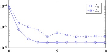
1 Introduction
Amongst the classical problems of fluid mechanics is the Stokes flow about a spherical particle settling in a viscous fluid. Particles of higher density (
 $\hat{\unicode[STIX]{x1D70C}}_{p}$
) than the fluid (
 $\hat{\unicode[STIX]{x1D70C}}_{f}$
) settle at a speed proportional to the density difference, gravitational acceleration (
 ${\hat{g}}$
) and particle diameter (
 $\hat{D}$
), but inversely proportional to the fluid viscosity. Viscoplastic fluids are generalized Newtonian fluids, i.e. the effective viscosity varies with strain rate. As the strain rate is induced by the buoyancy force, it is natural that the settling speed should vary nonlinearly with
 $(\hat{\unicode[STIX]{x1D70C}}_{p}-\hat{\unicode[STIX]{x1D70C}}_{f})$
. An additional feature of viscoplastic fluids is that they exhibit a yield stress,
 $\hat{\unicode[STIX]{x1D70F}}_{Y}$
, i.e. a stress below which the strain rate becomes zero. In the particle settling context, the settling speed is found to vanish if
 $(\hat{\unicode[STIX]{x1D70C}}_{p}-\hat{\unicode[STIX]{x1D70C}}_{f})$
is not sufficiently large. More precisely, the settling motion is driven by a buoyancy stress
 $(\hat{\unicode[STIX]{x1D70C}}_{p}-\hat{\unicode[STIX]{x1D70C}}_{f}){\hat{g}}\hat{D}$
, and if the ratio
 $Y=\hat{\unicode[STIX]{x1D70F}}_{Y}/[(\hat{\unicode[STIX]{x1D70C}}_{p}-\hat{\unicode[STIX]{x1D70C}}_{f}){\hat{g}}\hat{D}]$
is sufficiently large, the fluid does not yield and there is no particle motion:
 $Y>Y_{c}$
. The critical limit (
 $Y=Y_{c}$
) for a sphere was identified by Beris et al. (Reference Beris, Tsamopoulos, Armstrong and Brown1985), and
 $Y_{c}$
is known for various other geometries that we review below.
In drilling oil and gas wells, yield-stress fluids (drilling muds) are circulated around the wellbore, used to lubricate the drillpipe and drillbit, and to aid in removal of rock cuttings from the well to the surface (Okrajni & Azar Reference Okrajni and Azar1986; Elgaddafi et al.
Reference Elgaddafi, Ahmed, George and Growcock2012; Xiaofeng et al.
Reference Xiaofeng, Kelin, Tie, Yang, Shuai and Shizhu2013). When the drilling mud is circulating, the yield stress contributes to the viscous drag on the rock cuttings, enhancing transport. However, when circulation is stopped (as routinely happens), the more critical role of the yield stress is in preventing settling in the well, requiring
 $Y>Y_{c}$
. In such applications, proximity of other particles affects both
 $Y_{c}$
and drag, as studied, for example, by Liu, Muller & Denn (Reference Liu, Muller and Denn2003) and Merkak, Jossic & Magnin (Reference Merkak, Jossic and Magnin2006) in model situations. Equally, particle shape is a significant influence (Jossic & Magnin Reference Jossic and Magnin2001).
Other applications of more direct interest include the use of yield-stress fluids as an aid to fractionation of suspensions (Madani et al.
Reference Madani, Storey, Olson, Frigaard, Salmela and Martinez2010). These methods rely on our being able to use
 $Y_{c}$
to differentiate particle shape, size, density and orientation, for which there is little systematic study. This paper partly addresses this gap. It studies the effects of particle shape on
 $Y_{c}$
, systematically about symmetric particles in two-dimensional (2D) planar flows, and studies the approach to this limit. The critical value
 $Y_{c}$
in 2D planar flows has been computed for the circular disc (Tokpavi, Magnin & Jay Reference Tokpavi, Magnin and Jay2008), the square (Nirmalkar, Chhabra & Poole Reference Nirmalkar, Chhabra and Poole2012) and the ellipse (Putz & Frigaard Reference Putz and Frigaard2010). The main question is whether there are generic features of these flows that will allow us to calculate (or approximate)
 $Y_{c}$
for general configurations.
There are two ways of studying particle motion, and hence the limiting flows. One may impose the particle velocity and calculate the force on the particle: the resistance problem [R]. Alternatively, one imposes the (buoyancy) force on the particle and calculates the (settling) velocity. If the particle velocity is non-zero, there is a one-to-one correspondence between these two problems (Putz & Frigaard Reference Putz and Frigaard2010). Either method may be used to calculate the plastic drag coefficient, which approaches a constant value when the particle motion is stopped.
Variational methods were used in Putz & Frigaard (Reference Putz and Frigaard2010) to show that in the critical limit of zero flow the viscous dissipation converges at least one order of magnitude faster than the plastic dissipation, which balances with the rate of work due to the buoyancy forces. This prompts one to consider a (potentially simplified) flow problem in which the viscous terms are ignored, but not the yield-stress terms, which enters the realm of perfect plasticity (Hill Reference Hill1950). Although Beris et al. (Reference Beris, Tsamopoulos, Armstrong and Brown1985), Tokpavi et al. (Reference Tokpavi, Magnin and Jay2008) and Putz & Frigaard (Reference Putz and Frigaard2010) have all pointed to the potential advantages of using plasticity theory and especially the characteristics/slipline method for analysing the yield limit of the particle motion in viscoplastic fluids, no in-depth systematic attempts have been made. One of the best non-trivial examples of using the characteristics method for calculation of the collapse load is the study of Randolph & Houlsby (Reference Randolph and Houlsby1984), who constructed the characteristic network around a circular pile to calculate the lateral resistance to pushing the pile through surrounding soil. The more recent studies of Tokpavi et al. (Reference Tokpavi, Magnin and Jay2008) and Putz & Frigaard (Reference Putz and Frigaard2010) calculated the plastic drag coefficient numerically for a circular cylinder moving in a Bingham fluid and reported the same limiting drag coefficient as given by the analysis of Randolph & Houlsby (Reference Randolph and Houlsby1984), for the fully rough pile. This leads to hope that the characteristics method might be more widely applicable. However, later attempts to predict the limiting drag force by the characteristics theory were not successful. In Putz & Frigaard (Reference Putz and Frigaard2010) the numerical calculations for long prolate ellipses differ considerably from those that they calculated by generalizing the Randolph & Houlsby (Reference Randolph and Houlsby1984) expression. Nirmalkar et al. (Reference Nirmalkar, Chhabra and Poole2012) calculated drag coefficients that are not close to the estimates of Knappett, Mohammadi & Griffin (Reference Knappett, Mohammadi and Griffin2010).
The above status prompts us in this paper to revisit the relevance of perfect plasticity to the limiting flows of planar 2D particles. In doing so it should be noted that this is a two-part proposition. Firstly, if the characteristic network is calculated, then the stress field leads to a lower-bound estimate of the plastic drag coefficient (for the perfectly plastic flow). An upper-bound estimate can be derived from any admissible velocity field, but here the method is not straightforward for some geometries. It is only if the two estimates produce the same dissipation functional that the calculated drag coefficients are exact for the perfectly plastic flow, e.g. as with Randolph & Houlsby (Reference Randolph and Houlsby1984). Also note that the characteristics method in this context is simply a convenient method for generating an admissible stress tensor. Secondly, there is the question of comparison of the perfectly plastic drag coefficient with the limiting plastic drag coefficient. This latter comparison is positive for the circular disc, but in general only the normal velocity conditions are needed at the particle surface, to define velocity admissibility for the perfectly plastic flow. Hence there is no reason to suppose general agreement.
Apart from the use of the characteristics method within the variational context described above, usage of upper and lower bounds within the variational theory of viscoplastic fluids was pioneered in a series of papers by Adachi and Yoshioka (see Adachi & Yoshioka Reference Adachi and Yoshioka1973). However, although interesting qualitative understanding can be found in their analysis, the discrepancy between their two bounds was relatively large. Moreover, generalizing their method to make quantitative estimates for more general geometries does not seem straightforward, i.e. in comparison to using the characteristic network for different geometries.
Critical yield numbers are not only a feature of particle settling in yield-stress fluids, as many other flows involve a balance between an imposed force (stress) and the yield stress. Thus flow onset below a suitably defined critical
 $Y$
is an essential feature of very many viscoplastic flows, including the most simple one-dimensional (1D) flows, such as Poiseuille flows in pipes and plane channels or uniform film flows, e.g. paint on a vertical wall. Since the critical
 $Y$
does not involve viscosity, it is self-evident that the same
 $Y_{c}$
will be found for any yield-stress fluid where yielding uses the von Mises criterion. Thus, here we consider the simplest such fluid: a Bingham fluid.
The first systematic study of critical yield numbers was carried out by Mosolov & Miasnikov (Reference Mosolov and Miasnikov1965, Reference Mosolov and Miasnikov1966), who considered antiplane shear flows, i.e. flows with velocity
 $\boldsymbol{u}=(0,0,w(x_{1},x_{2}))$
in the
 $x_{3}$
-direction along ducts (infinite cylinders) of arbitrary cross-section. These flows driven by a constant pressure gradient only admit the static solution (
 $w=0$
) if the yield stress is sufficiently large. Amongst the many interesting results in their works, the key contributions relate to exposing the strongly geometric nature of calculating the critical yield number
 $Y_{c}$
. Firstly, they show that
 $Y_{c}$
can be related to the maximal ratio of area to perimeter of subsets of the cross-section
 $\unicode[STIX]{x1D6FA}$
. Secondly, they develop an algorithmic methodology for calculating
 $Y_{c}$
for specific symmetric
 $\unicode[STIX]{x1D6FA}$
, e.g. rectangular ducts. This methodology is extended further by Huilgol (Reference Huilgol2006).
The context of settling particles in antiplane shear flows (meaning infinitely long solid cylinders within
 $\unicode[STIX]{x1D6FA}$
) has recently been analysed by Frigaard et al. (Reference Frigaard, Iglesias, Mercier, Pöschl and Scherzer2017). As with Mosolov & Miasnikov (Reference Mosolov and Miasnikov1965, Reference Mosolov and Miasnikov1966), these limiting flows may be evaluated geometrically and calculated exactly for many simple particle and fluid domain shapes. Unlike the flows considered here, the limiting flows are non-local, affecting the entire fluid domain.
Critical yield numbers have also been studied for many other flows, using analytical estimates, computational approximations and experimentation. Critical yield numbers to prevent bubble motion are considered in Dubash & Frigaard (Reference Dubash and Frigaard2004) and Tsamopoulos et al. (Reference Tsamopoulos, Dimakopoulos, Chatzidai, Karapetsas and Pavlidis2008). Natural convection is studied in Karimfazli & Frigaard (Reference Karimfazli and Frigaard2013) and Karimfazli, Frigaard & Wachs (Reference Karimfazli, Frigaard and Wachs2015). The onset of landslides are studied in Hild et al. (Reference Hild, Ionescu, Lachand-Robert and Roşca2002), Hassani, Ionescu & Lachand-Robert (Reference Hassani, Ionescu and Lachand-Robert2005) and Ionescu & Lachand-Robert (Reference Ionescu and Lachand-Robert2005) (where the terminologies ‘load limit analysis’ and ‘blocking solutions’ have also been used). Stepping away from the Stokes flow context, it is worth mentioning that the critical
 $Y_{c}$
also serves as a stability limit for transient flows, including those with inertia. This is true both for single-particle flows (Wachs & Frigaard Reference Wachs and Frigaard2016) and for wide classes of interior flows (Karimfazli & Frigaard Reference Karimfazli and Frigaard2016). Thus, determination of
 $Y_{c}$
has additional significance.
To summarize, the main focus of our paper is the systematic study of the effects of shape and aspect ratio on the limiting 2D flows of planar symmetric particles through a Bingham fluid. To this end, we use computations of the viscoplastic flows, characteristics theory for comparable plastic flows and a range of analytical tools. An outline of our paper is as follows. In § 2 we set out the general problem studied, introduce the variational terminology, the characteristics method and other basic features. Then § 3 presents the main results. We start by re-examining the circular cylinder flow of Tokpavi et al. (Reference Tokpavi, Magnin and Jay2008) and Putz & Frigaard (Reference Putz and Frigaard2010) and the characteristics solution of Randolph & Houlsby (Reference Randolph and Houlsby1984), showing the differences in the solutions even though the limiting plastic drag coefficients agree. This prompts examination of three families of particles, i.e. ellipses, rectangles and diamonds, from the perspectives of both viscoplastic flows and characteristics. We find that the lower-bound characteristics method generally gives an accurate approximation to
 $Y_{c}$
, but is only exact for certain specific geometries. In § 4 we explore the characteristics of particles with large and small aspect ratio
 $\unicode[STIX]{x1D712}$
, and also those of flows in the limit
 $Y\rightarrow Y_{c}$
. The paper ends with a brief discussion.
2 Problem statement
This paper focuses on the motion of isolated symmetric 2D particles in a viscoplastic medium. The flow is assumed to be inertialess and isothermal. The particle is denoted by
 $X$
;
 $\unicode[STIX]{x2202}X$
is the boundary of the particle; and
 $\unicode[STIX]{x1D6FA}$
and
 $\unicode[STIX]{x2202}\unicode[STIX]{x1D6FA}$
represent the entire domain (fluid
 $+$
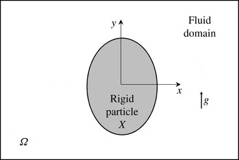
particle) and its outer boundary, respectively (see figure 1). Of particular interest are flows in which the particle is just able to move. We formulate this problem based on the motion being driven by buoyancy (mobility problem, [M]), later introducing the equivalent problem based on imposed particle motion (resistance problem, [R]).
Two-dimensional schematic of the particle motion.

We assume the particle is denser than the fluid,
 $\hat{\unicode[STIX]{x1D70C}}_{p}>\hat{\unicode[STIX]{x1D70C}}_{f}$
, and align the gravitational acceleration with the positive
 $y$
-direction,
 ${\hat{g}}\boldsymbol{e}_{y}$
. Considering a circular disc as a reference geometry, we select a length scale
 $\hat{L}$
such that
 $$\begin{eqnarray}\displaystyle \unicode[STIX]{x03C0}\hat{L}^{2}=\int _{X}\text{d}\hat{x}\,\text{d}{\hat{y}}=\text{area of }X, & & \displaystyle\end{eqnarray}$$
i.e.
 $\hat{L}$
is the radius if
 $X$
is circular. A representative buoyancy stress is therefore
 $\hat{\unicode[STIX]{x1D70F}}_{b}=(\hat{\unicode[STIX]{x1D70C}}_{p}-\hat{\unicode[STIX]{x1D70C}}_{f}){\hat{g}}\hat{L}$
. We use
 $\hat{\unicode[STIX]{x1D70F}}_{b}$
to scale the flow, starting with the definition of the velocity scale
 $\hat{U} _{b}$
, selected to balance
 $\hat{\unicode[STIX]{x1D70F}}_{b}$
with the viscous stress:
 $$\begin{eqnarray}\frac{\hat{\unicode[STIX]{x1D707}}\hat{U} _{b}}{\hat{L}}=\hat{\unicode[STIX]{x1D70F}}_{b}\quad \Rightarrow \quad \hat{U} _{b}=\frac{(\hat{\unicode[STIX]{x1D70C}}_{p}-\hat{\unicode[STIX]{x1D70C}}_{f}){\hat{g}}\hat{L}^{2}}{\hat{\unicode[STIX]{x1D707}}},\end{eqnarray}$$
where
 $\hat{\unicode[STIX]{x1D707}}$
is the plastic viscosity.
On scaling the Stokes equations with
 $\hat{\unicode[STIX]{x1D70F}}_{b}/\hat{L}$
, we find
 $$\begin{eqnarray}\displaystyle & \displaystyle \unicode[STIX]{x1D735}\boldsymbol{\cdot }\unicode[STIX]{x1D748}+\frac{\unicode[STIX]{x1D70C}}{1-\unicode[STIX]{x1D70C}}\boldsymbol{e}_{y}=0\quad \text{in}~\unicode[STIX]{x1D6FA}\setminus \bar{X}, & \displaystyle\end{eqnarray}$$
 $$\begin{eqnarray}\displaystyle & \displaystyle \unicode[STIX]{x1D735}\boldsymbol{\cdot }\boldsymbol{u}=0\quad \text{in}~\unicode[STIX]{x1D6FA}\setminus \bar{X}, & \displaystyle\end{eqnarray}$$
 $\unicode[STIX]{x1D748}$
is the Cauchy stress tensor,
 $\boldsymbol{u}$
is the velocity and
 $\unicode[STIX]{x1D70C}=\hat{\unicode[STIX]{x1D70C}}_{f}/\hat{\unicode[STIX]{x1D70C}}_{p}$
. The stress tensor can be written as
 $\unicode[STIX]{x1D748}=-p\unicode[STIX]{x1D739}+\unicode[STIX]{x1D749}$
, where
 $\unicode[STIX]{x1D749}$
is the deviatoric stress tensor,
 $p$
is the pressure and
 $\unicode[STIX]{x1D739}$
is the Kronecker delta. As we study the limit of yielding/flow, the viscous behaviour after yielding is of secondary interest. Consequently, we consider the simplest constitutive model, i.e. a Bingham fluid:
 $$\begin{eqnarray}\left.\begin{array}{@{}c@{}}\unicode[STIX]{x1D749}=\left(1+\displaystyle \frac{Y}{\Vert \dot{\unicode[STIX]{x1D738}}\Vert }\right)\dot{\unicode[STIX]{x1D738}}\quad \text{if}~\Vert \unicode[STIX]{x1D749}\Vert >Y,\\ \dot{\unicode[STIX]{x1D738}}=0\quad \text{if}~\Vert \unicode[STIX]{x1D749}\Vert \leqslant Y,\end{array}\right\}\end{eqnarray}$$
where
 $Y=\hat{\unicode[STIX]{x1D70F}}_{Y}\hat{L}/\hat{\unicode[STIX]{x1D707}}\hat{U} _{b}=\hat{\unicode[STIX]{x1D70F}}_{Y}/(\hat{\unicode[STIX]{x1D70C}}_{p}-\hat{\unicode[STIX]{x1D70C}}_{f}){\hat{g}}\hat{L}$
is the yield number (sometimes also called the gravity yield number). Here
 $\hat{\unicode[STIX]{x1D70F}}_{Y}$
is the yield stress of the Bingham fluid and hence
 $Y$
is the ratio of yield stress to buoyancy stress. In (2.4)
 $\dot{\unicode[STIX]{x1D738}}$
is the strain-rate tensor and
 $\Vert \cdot \Vert$
is the norm associated with the tensor inner product:
 $$\begin{eqnarray}\displaystyle \boldsymbol{c}\boldsymbol{ : }\boldsymbol{d}=\frac{1}{2}\mathop{\sum }_{ij}c_{ij}d_{ij}, & & \displaystyle\end{eqnarray}$$
e.g.
 $\Vert \unicode[STIX]{x1D749}\Vert =(\unicode[STIX]{x1D749}\boldsymbol{ : }\unicode[STIX]{x1D749})^{1/2}$
. We use subscripts in the conventional Einstein summation notation. Throughout the paper, quantities with a ‘hat’ symbol
 $(\hat{\cdot })$
are dimensional and others are dimensionless.
Regarding the boundary conditions, in the far field we specify
 $$\begin{eqnarray}\boldsymbol{u}=0\quad \text{on }\unicode[STIX]{x2202}\unicode[STIX]{x1D6FA}\setminus \unicode[STIX]{x2202}X.\end{eqnarray}$$
Note that for yield-stress fluids such as (2.4), as soon as the stress
 $(\Vert \unicode[STIX]{x1D749}\Vert )$
decays below
 $Y$
, the fluid becomes rigid. Thus, typically there is a bounded yielded region formed near to the particle which is surrounded by outer rigid fluid (unyielded). Although the extent of the yielded region is not known a priori, the fact that it exists means that equality can be imposed in (2.6), instead of a far-field decay rate at
 $\infty$
. Practically, we may consider (2.6) to be imposed at a rigid wall, which guarantees that the unyielded fluid is static. Choosing an appropriate
 $\unicode[STIX]{x2202}\unicode[STIX]{x1D6FA}$
can significantly reduce the computational cost of the problem.
At the particle surface
 $\unicode[STIX]{x2202}X$
, the fluid velocity is continuous with that of the particle:
 $$\begin{eqnarray}\boldsymbol{u}\rightarrow \boldsymbol{U}\quad \text{on }\unicode[STIX]{x2202}X,\end{eqnarray}$$
but
 $\boldsymbol{U}$
is unknown. In this paper we consider only particles that are settling in the
 $y$
-direction. Provided the particles have two orthogonal symmetry planes, there is no torque exerted on the particle and only linear motion of the particle is possible. Provided that the symmetry axes orient with
 $\boldsymbol{e}_{y}$
, there is no drift component of velocity. Thus, we may write
 $\boldsymbol{U}=U\boldsymbol{e}_{y}$
.
The stress at the particle surface must satisfy the following force balance:
 $$\begin{eqnarray}\int _{\unicode[STIX]{x2202}X}\unicode[STIX]{x1D748}\boldsymbol{\cdot }\boldsymbol{n}\,\text{d}s=\frac{\unicode[STIX]{x03C0}}{1-\unicode[STIX]{x1D70C}}\boldsymbol{e}_{y},\end{eqnarray}$$
where
 $\boldsymbol{n}$
is the normal of
 $\unicode[STIX]{x2202}X$
, pointing inwards to the particle (recall that
 $\unicode[STIX]{x03C0}$
is the dimensionless area of the particle). Note here that the net force (per unit length) is also in the
 $y$
-direction, by consequence of the force equilibrium in the
 $x$
-direction and the symmetry of the particles.
Note that since the particle velocity
 $\boldsymbol{U}$
is also divergence-free, there is no net volumetric flux across
 $\unicode[STIX]{x1D6FA}$
in any direction. A particular consequence of this is
 $$\begin{eqnarray}\int _{\unicode[STIX]{x1D6FA}\setminus \bar{X}}\boldsymbol{u}\boldsymbol{\cdot }\boldsymbol{e}_{y}\,\text{d}A=-\int _{\bar{X}}\boldsymbol{U}\boldsymbol{\cdot }\boldsymbol{e}_{y}\,\text{d}A=-\unicode[STIX]{x03C0}\boldsymbol{U}\boldsymbol{\cdot }\boldsymbol{e}_{y}=-\unicode[STIX]{x03C0}U.\end{eqnarray}$$
2.1 Variational tools
The energy equation and two variational principles are useful in calculating the solution and studying limiting flows. Firstly, let us consider the space of admissible velocity solutions:
 $$\begin{eqnarray}\displaystyle {\mathcal{V}}=\{\boldsymbol{v}\boldsymbol{ : }\unicode[STIX]{x1D735}\boldsymbol{\cdot }\boldsymbol{v}=0~\text{in }\unicode[STIX]{x1D6FA}\setminus \bar{X};~\boldsymbol{v}=0~\text{on }\unicode[STIX]{x2202}\unicode[STIX]{x1D6FA}\setminus \unicode[STIX]{x2202}X;~\boldsymbol{v}\rightarrow \boldsymbol{V}=V\boldsymbol{e}_{y}~\text{on }\unicode[STIX]{x2202}X\}, & & \displaystyle\end{eqnarray}$$
where
 $\boldsymbol{V}$
is an unspecified constant particle test velocity. For arbitrary
 $\boldsymbol{v},\boldsymbol{w}\in {\mathcal{V}}$
, the viscous dissipation, plastic dissipation and buoyancy work functionals, respectively, are
 $$\begin{eqnarray}\displaystyle & \displaystyle a(\boldsymbol{v},\boldsymbol{w})=\int _{\unicode[STIX]{x1D6FA}\setminus \bar{X}}\dot{\unicode[STIX]{x1D738}}(\boldsymbol{v})\boldsymbol{ : }\dot{\unicode[STIX]{x1D738}}(\boldsymbol{w})\,\text{d}A, & \displaystyle\end{eqnarray}$$
 $$\begin{eqnarray}\displaystyle & \displaystyle j(\boldsymbol{v})=\int _{\unicode[STIX]{x1D6FA}\setminus \bar{X}}\Vert \dot{\unicode[STIX]{x1D738}}(\boldsymbol{v})\Vert \,\text{d}A, & \displaystyle\end{eqnarray}$$
 $$\begin{eqnarray}\displaystyle & \displaystyle L(\boldsymbol{v})=\unicode[STIX]{x03C0}V=\unicode[STIX]{x03C0}\boldsymbol{V}\boldsymbol{\cdot }\boldsymbol{e}_{y}=-\int _{\unicode[STIX]{x1D6FA}\setminus \bar{X}}\boldsymbol{v}\boldsymbol{\cdot }\boldsymbol{e}_{y}\,\text{d}A. & \displaystyle\end{eqnarray}$$
 $\unicode[STIX]{x1D6FA}\setminus \bar{X}$
. On using the divergence theorem, (2.8) and (2.9), we find
 $$\begin{eqnarray}\displaystyle a(\boldsymbol{u},\boldsymbol{u})+Y\,j(\boldsymbol{u}) & = & \displaystyle \frac{\unicode[STIX]{x1D70C}}{1-\unicode[STIX]{x1D70C}}\int _{\unicode[STIX]{x1D6FA}\setminus \bar{X}}\boldsymbol{u}\boldsymbol{\cdot }\boldsymbol{e}_{y}\,\text{d}A+\int _{\unicode[STIX]{x2202}X}\boldsymbol{u}\boldsymbol{\cdot }\unicode[STIX]{x1D748}\boldsymbol{\cdot }\boldsymbol{n}\,\text{d}s\nonumber\\ \displaystyle & = & \displaystyle -\frac{\unicode[STIX]{x1D70C}}{1-\unicode[STIX]{x1D70C}}\int _{\bar{X}}\boldsymbol{U}\boldsymbol{\cdot }\boldsymbol{e}_{y}\,\text{d}A+\int _{\unicode[STIX]{x2202}X}\boldsymbol{U}\boldsymbol{\cdot }\unicode[STIX]{x1D748}\boldsymbol{\cdot }\boldsymbol{n}\,\text{d}s\nonumber\\ \displaystyle & = & \displaystyle -\frac{\unicode[STIX]{x03C0}\unicode[STIX]{x1D70C}}{1-\unicode[STIX]{x1D70C}}\boldsymbol{U}\boldsymbol{\cdot }\boldsymbol{e}_{y}+\boldsymbol{U}\boldsymbol{\cdot }\int _{\unicode[STIX]{x2202}X}\unicode[STIX]{x1D748}\boldsymbol{\cdot }\boldsymbol{n}\,\text{d}s=\unicode[STIX]{x03C0}U=L(\boldsymbol{u}).\end{eqnarray}$$
Below, (2.12) is used to define the critical yield number.
The velocity minimization principle states that the solution
 $\boldsymbol{u}$
minimizes the functional
 ${\mathcal{J}}(\boldsymbol{v})$
over
 $\boldsymbol{v}\in {\mathcal{V}}$
:
 $$\begin{eqnarray}{\mathcal{J}}(\boldsymbol{v})=\frac{1}{2}a(\boldsymbol{v},\boldsymbol{v})+Y\,j(\boldsymbol{v})-\frac{\unicode[STIX]{x1D70C}}{1-\unicode[STIX]{x1D70C}}\int _{\unicode[STIX]{x1D6FA}\setminus \bar{X}}\boldsymbol{v}\boldsymbol{\cdot }\boldsymbol{e}_{y}\,\text{d}A-\int _{\unicode[STIX]{x2202}X}\unicode[STIX]{x1D70E}_{ij}(\boldsymbol{u})n_{j}V_{i}\,\text{d}s.\end{eqnarray}$$
Note that the traction of the solution at the particle surface (contained within the last term on the right-hand side) satisfies (2.8). Since
 $\boldsymbol{V}$
is constant, (2.9) applies to the pairing
 $(\boldsymbol{v},\boldsymbol{V})$
, and on using (2.8) we obtain
 $$\begin{eqnarray}\displaystyle -\frac{\unicode[STIX]{x1D70C}}{1-\unicode[STIX]{x1D70C}}\int _{\unicode[STIX]{x1D6FA}\setminus \bar{X}}\boldsymbol{v}\boldsymbol{\cdot }\boldsymbol{e}_{y}\,\text{d}A-\int _{\unicode[STIX]{x2202}X}\unicode[STIX]{x1D70E}_{ij}(\boldsymbol{u})n_{j}V_{i}\,\text{d}s=\frac{\unicode[STIX]{x03C0}\unicode[STIX]{x1D70C}V}{1-\unicode[STIX]{x1D70C}}-\boldsymbol{V}\boldsymbol{\cdot }\int _{\unicode[STIX]{x2202}X}\unicode[STIX]{x1D748}(\boldsymbol{u})\boldsymbol{\cdot }\boldsymbol{n}\,\text{d}s=-L(\boldsymbol{v}), & & \displaystyle \nonumber\\ \displaystyle & & \displaystyle\end{eqnarray}$$
so that equivalently
 ${\mathcal{J}}(\boldsymbol{v})=(1/2)a(\boldsymbol{v},\boldsymbol{v})+Y\,j(\boldsymbol{v})-L(\boldsymbol{v})$
.
For the second variational principle, consider the space of admissible stresses
 ${\mathcal{S}}$
:
 $$\begin{eqnarray}\displaystyle {\mathcal{S}}=\left\{\unicode[STIX]{x1D748}^{\prime }=\unicode[STIX]{x1D749}^{\prime }-p^{\prime }\boldsymbol{I}\boldsymbol{ : }\unicode[STIX]{x1D735}\boldsymbol{\cdot }\unicode[STIX]{x1D748}^{\prime }+\frac{\unicode[STIX]{x1D70C}}{1-\unicode[STIX]{x1D70C}}\boldsymbol{e}_{y}=0~\text{in }\unicode[STIX]{x1D6FA}\setminus \bar{X};~\int _{\unicode[STIX]{x2202}X}\unicode[STIX]{x1D748}^{\prime }\boldsymbol{\cdot }\boldsymbol{n}\,\text{d}s=\frac{\unicode[STIX]{x03C0}}{1-\unicode[STIX]{x1D70C}}\boldsymbol{e}_{y}\right\}, & & \displaystyle \nonumber\\ \displaystyle & & \displaystyle\end{eqnarray}$$
i.e. symmetric stress tensors satisfying the Stokes equations and the force balance (2.8). The solution
 $\unicode[STIX]{x1D748}$
maximizes over
 $\unicode[STIX]{x1D748}^{\prime }\in {\mathcal{S}}$
the functional
 $$\begin{eqnarray}{\mathcal{K}}(\unicode[STIX]{x1D748}^{\prime })=\int _{\unicode[STIX]{x2202}X}\unicode[STIX]{x1D70E}_{ij}^{\prime }n_{j}U_{i}\,\text{d}s-\frac{1}{2}\int _{\unicode[STIX]{x1D6FA}\setminus \bar{X}}(\Vert \unicode[STIX]{x1D749}^{\prime }\Vert -Y)_{+}^{2}\,\text{d}A,\end{eqnarray}$$
where
 $(f)_{+}$
denotes the positive part of
 $f$
. Furthermore, for any admissible velocity and stress we have
 $$\begin{eqnarray}{\mathcal{K}}(\unicode[STIX]{x1D748}^{\prime })\leqslant {\mathcal{K}}(\unicode[STIX]{x1D748})={\mathcal{J}}(\boldsymbol{u})\leqslant {\mathcal{J}}(\boldsymbol{v}).\end{eqnarray}$$
These results date back to Prager (Reference Prager1954). A general derivation is explained at length in Huilgol (Reference Huilgol2015).
2.2 Yielding of flows
An important feature of yield-stress fluids is their ability to hold particles statically stable under certain circumstances. From the physical perspective, as discussed in our scaling, the density difference between particle and fluid leads to shear stresses of order
 $\hat{\unicode[STIX]{x1D70F}}_{b}=(\hat{\unicode[STIX]{x1D70C}}_{p}-\hat{\unicode[STIX]{x1D70C}}_{f}){\hat{g}}\hat{L}$
. It is physically intuitive that, if the yield stress
 $\hat{\unicode[STIX]{x1D70F}}_{Y}$
is sufficiently large (implicitly meaning
 $\hat{\unicode[STIX]{x1D70F}}_{Y}\gg (\hat{\unicode[STIX]{x1D70C}}_{p}-\hat{\unicode[STIX]{x1D70C}}_{f}){\hat{g}}\hat{L}$
), then the yield stress will not be exceeded anywhere in the flow. Since the velocity is zero on
 $\unicode[STIX]{x2202}\unicode[STIX]{x1D6FA}$
there would then be no motion in the fluid and hence no motion of the particle. The ratio
 $\hat{\unicode[STIX]{x1D70F}}_{Y}/\hat{\unicode[STIX]{x1D70F}}_{b}$
is the yield number and the above argument predicts stationary flow for sufficiently large
 $Y$
. We can verify this intuition analytically, using the tools of the previous section (see e.g. Putz & Frigaard Reference Putz and Frigaard2010).
Secondly, we might re-examine the maximization (2.16). Since each admissible
 $\unicode[STIX]{x1D748}^{\prime }$
satisfies (2.8), we may also write
 $$\begin{eqnarray}{\mathcal{K}}(\unicode[STIX]{x1D748}^{\prime })=\frac{1}{1-\unicode[STIX]{x1D70C}}L(\boldsymbol{u})-\frac{1}{2}\int _{\unicode[STIX]{x1D6FA}\setminus \bar{X}}(\Vert \unicode[STIX]{x1D749}^{\prime }\Vert -Y)_{+}^{2}\,\text{d}A.\end{eqnarray}$$
The first term is independent of
 $\unicode[STIX]{x1D748}^{\prime }\in {\mathcal{S}}$
and the second term is negative definite. Any admissible stress field with
 $\Vert \unicode[STIX]{x1D749}^{\prime }\Vert \leqslant Y$
will therefore maximize
 ${\mathcal{K}}$
. Equally, if any such
 $\unicode[STIX]{x1D748}^{\prime }\in {\mathcal{S}}$
can be found, then it follows that the true stress must also have
 $\Vert \unicode[STIX]{x1D749}\Vert \leqslant Y$
. This in turn implies that the solution stress does not exceed the yield stress, hence that the strain rate is zero everywhere, and consequently that
 $\boldsymbol{u}=0$
. Via the equivalence (2.17), we see that
 ${\mathcal{K}}(\unicode[STIX]{x1D748})={\mathcal{J}}(\boldsymbol{u})=0$
, in this limit. Thus, the condition for the particle not to yield the fluid is independent of the precise type of fluid (Bingham, Casson, Herschel–Bulkley, Robertson–Stiff, etc.): any viscoplastic fluid remains preferentially static.
The energy equation can be used to define the minimal limiting yield stress for static flow, via a critical value of
 $Y$
:
 $$\begin{eqnarray}Y_{c}=\sup _{\boldsymbol{v}\in {\mathcal{V}},\,\boldsymbol{v}\not =0}\frac{L(\boldsymbol{v})}{j(\boldsymbol{v})},\end{eqnarray}$$
with
 $\boldsymbol{u}=\boldsymbol{U}=0$
if
 $Y\geqslant Y_{c}$
(Putz & Frigaard Reference Putz and Frigaard2010). The variational form of the velocity minimization can then be used to show that as
 $Y\rightarrow Y_{c}^{-}$
the viscous dissipation of the solution
 $\boldsymbol{u}$
will decay at least one order faster than the plastic dissipation. More precisely, as
 $Y\rightarrow Y_{c}^{-}$
,
 $$\begin{eqnarray}\displaystyle a(\boldsymbol{u},\boldsymbol{u})=O([Y_{c}-Y]^{2}),\quad j(\boldsymbol{u})=O(Y_{c}-Y), & & \displaystyle\end{eqnarray}$$
 $$\begin{eqnarray}\displaystyle \frac{a(\boldsymbol{u},\boldsymbol{u})}{j(\boldsymbol{u})}=O(Y_{c}-Y). & & \displaystyle\end{eqnarray}$$
Returning to (2.12), we see that the plastic dissipation must balance with the buoyancy work as
 $Y\rightarrow Y_{c}^{-}$
, i.e.
 $$\begin{eqnarray}Y\,j(\boldsymbol{u})\sim L(\boldsymbol{u})=\unicode[STIX]{x03C0}U,\end{eqnarray}$$
giving us directly the decay of the settling velocity as
 $Y\rightarrow Y_{c}^{-}$
.
2.3 Resistance formulation
The formulation [M] adopted is as a mobility problem. A different formulation is as a resistance problem [R], where we suppose that a constant particle velocity
 $\hat{\boldsymbol{U}}_{p}$
is imposed and the force on the particle
 $\hat{\boldsymbol{F}}$
is measured. The particle velocity scales the velocity and is used to define a viscous stress scale
 $\hat{\unicode[STIX]{x1D70F}}_{p}=\hat{\unicode[STIX]{x1D707}}\hat{U} _{p}/\hat{L}$
, with which the Stokes equations are scaled:
 $$\begin{eqnarray}\unicode[STIX]{x1D735}\boldsymbol{\cdot }\unicode[STIX]{x1D748}^{\ast }=0,\quad \unicode[STIX]{x1D735}\boldsymbol{\cdot }\boldsymbol{u}^{\ast }=0\quad \text{in }\unicode[STIX]{x1D6FA}\setminus \bar{X}.\end{eqnarray}$$
Lengths are scaled as previously. The ‘asterisk’ is used to distinguish variables from the [M]-scaled variables, where needed. No body forces are present in the fluid domain. The constitutive laws are again (2.4) with
 $Y$
replaced by
 $B$
, which is the Bingham number:
 $B=\hat{\unicode[STIX]{x1D70F}}_{Y}\hat{L}/\hat{\unicode[STIX]{x1D707}}\hat{U} _{p}$
. The motion is driven only by boundary conditions on the particle, i.e.
 $\boldsymbol{u}^{\ast }=\boldsymbol{e}_{y}$
on
 $\unicode[STIX]{x2202}X$
.
In order to have a correspondence between problems [M] and [R], we align the direction of particle motion with
 $\boldsymbol{e}_{y}$
, assumed to be a symmetry axis of the particle. The mapping between problems [M] and [R] is captured by
 $$\begin{eqnarray}\boldsymbol{u}=\frac{Y}{B}\boldsymbol{u}^{\ast },\quad U=\frac{Y}{B},\quad \unicode[STIX]{x03C0}\frac{B}{Y}=F^{\ast },\end{eqnarray}$$
where the scaled force exerted on the particle has magnitude
 $F^{\ast }$
and is in the direction
 $-\boldsymbol{e}_{y}$
.
One reason for introducing [R] is that it may be more convenient to compute the solution of problem [R] (rather than [M]), and use this to evaluate
 $Y_{c}$
. In controlling relative numerical errors, the velocities in problem [R] are strictly
 $O(1)$
. Secondly, as argued by Putz & Frigaard (Reference Putz and Frigaard2010), optimality of
 $L(\boldsymbol{v})/j(\boldsymbol{v})$
in (2.19) is attained by the solution
 $\boldsymbol{u}$
to [M], in the limit that
 $Y\rightarrow Y_{c}^{-}$
. On rescaling
 $\boldsymbol{u}$
with
 $U$
, we arrive at the equivalent solution to [R], for
 $B=Y/U$
. The functional
 $L(\boldsymbol{v})/j(\boldsymbol{v})$
in (2.19) also rescales and thus
 $Y_{c}$
may be calculated alternatively as
 $$\begin{eqnarray}Y_{c}=\lim _{Y\rightarrow Y_{c}^{-}}\frac{L(\boldsymbol{u})}{j(\boldsymbol{u})}=\lim _{Y\rightarrow Y_{c}^{-}}\frac{\unicode[STIX]{x03C0}U}{j(\boldsymbol{u})}=\lim _{B\rightarrow \infty }\frac{\unicode[STIX]{x03C0}}{j(\boldsymbol{u}^{\ast })}.\end{eqnarray}$$
Although finding the solution
 $\boldsymbol{u}^{\ast }$
, as
 $B\rightarrow \infty$
, may become numerically difficult, at least
 $j(\boldsymbol{u}^{\ast })$
is an integral quantity and should be more stable to compute than a pointwise quantity, allowing the asymptotic behaviour at large
 $B$
to be estimated effectively from a numerical solution.
2.4 The plastic drag coefficient
A different way of evaluating the critical stopping limit, which is useful for comparing between problems, involves the drag coefficient. Conventionally, a drag coefficient is defined by scaling the force on an object with an inertial stress scale and cross-sectional area. Here we consider inertialess flows close to yielding. The plastic drag coefficient instead uses the yield stress in place of an inertial stress. For the 2D flow, in either formulation:
 $$\begin{eqnarray}\displaystyle C_{D}^{p}=\left\{\begin{array}{@{}l@{}}\left[\displaystyle \frac{\hat{F}}{\hat{\ell }_{\bot }\hat{\unicode[STIX]{x1D70F}}_{Y}}\right]^{[R]}=\left[\displaystyle \frac{F^{\ast }}{\ell _{\bot }B}\right]^{[R]}\quad \text{for problem [R]},\quad \\ \left[\displaystyle \frac{\hat{\unicode[STIX]{x1D70C}}{\hat{g}}\hat{A}_{p}}{\hat{\ell }_{\bot }\hat{\unicode[STIX]{x1D70F}}_{Y}}\right]^{[M]}=\left[\displaystyle \frac{\unicode[STIX]{x03C0}}{\ell _{\bot }Y}\right]^{[M]}\quad \text{for problem [M]},\quad \end{array}\right. & & \displaystyle\end{eqnarray}$$
where
 $\hat{\ell }_{\bot }=\ell _{\bot }\hat{L}$
is the linear dimension of the particle perpendicular to the flow direction. Other similar problems may be compared by scaling the particle force
 $\hat{F}$
, as above with
 $\hat{\ell }_{\bot }\hat{\unicode[STIX]{x1D70F}}_{Y}$
. We see from the above again that
 $F^{\ast }=\unicode[STIX]{x03C0}B/Y$
. As we increase the yield stress and approach
 $Y\rightarrow Y_{c}^{-}$
, the plastic drag coefficient approaches a critical value:
 $$\begin{eqnarray}C_{D,c}^{p}=\frac{\unicode[STIX]{x03C0}}{\ell _{\bot }Y_{c}}=\left[C_{D}^{p}\right]_{Y\rightarrow Y_{c}^{-}}^{[M]}=\left[C_{D}^{p}\right]_{B\rightarrow \infty }^{[R]}.\end{eqnarray}$$
Critical values
 $C_{D,c}^{p}$
have been reported for various particles with simple geometry. For example, Tokpavi et al. (Reference Tokpavi, Magnin and Jay2008) calculated
 $C_{D,c}^{p}$
for a circular disc and Nirmalkar et al. (Reference Nirmalkar, Chhabra and Poole2012) calculated
 $C_{D,c}^{p}$
for a square. Both studies used the resistance formulation [R] and extrapolated to the critical value. Alternatively, Putz & Frigaard (Reference Putz and Frigaard2010) calculated
 $C_{D,c}^{p}$
for 2D elliptical particles using problem [M].
2.5 The yield limit and perfect plasticity
Under either formulation [M] or [R] we have seen that the viscous dissipation terms apparently play a minor role in the limit of zero flow. If we neglect the viscous terms in the constitutive law, in yielded regions we have
 $$\begin{eqnarray}\unicode[STIX]{x1D749}\approx B\frac{\dot{\unicode[STIX]{x1D738}}}{\Vert \dot{\unicode[STIX]{x1D738}}\Vert }.\end{eqnarray}$$
This is reminiscent of a rigid–perfectly plastic material (Hill Reference Hill1950), which may be considered as the limit of the Prandtl–Reuss model for perfectly plastic materials, in the case that the elastic modulus is infinitely large. The stress at no point can exceed the yield stress in (2.28). If the stress is strictly lower than the yield stress, the material is modelled as rigid, but formally (2.28) is an approximation in the limit of vanishingly small strain rates.
In a 2D flow, the steady momentum equations plus the von Mises yield criterion form a closed set of hyperbolic equations for the plastic regions of flow (see Chakrabarty Reference Chakrabarty2012). Considering now only problem [R] we have
 $$\begin{eqnarray}\displaystyle & \displaystyle \unicode[STIX]{x1D735}\boldsymbol{\cdot }\tilde{\unicode[STIX]{x1D749}}-\unicode[STIX]{x1D735}\tilde{p}=0, & \displaystyle\end{eqnarray}$$
 $$\begin{eqnarray}\displaystyle & \displaystyle \Vert \tilde{\unicode[STIX]{x1D749}}\Vert =B. & \displaystyle\end{eqnarray}$$
 $\unicode[STIX]{x1D6FC}$
-lines and
 $\unicode[STIX]{x1D6FD}$
-lines (sometimes referred to as sliplines). The stress at each point in the plastic region is represented by the pressure and an angle
 $\unicode[STIX]{x1D719}$
that represents the anticlockwise orientation that an
 $\unicode[STIX]{x1D6FC}$
-line makes with the
 $x$
-axis.
 $$\begin{eqnarray}\tilde{\unicode[STIX]{x1D70E}}_{xx}=-\tilde{p}-B\sin (2\unicode[STIX]{x1D719}),\quad \tilde{\unicode[STIX]{x1D70E}}_{yy}=-\tilde{p}+B\sin (2\unicode[STIX]{x1D719}),\quad \tilde{\unicode[STIX]{x1D70F}}_{xy}=B\cos (2\unicode[STIX]{x1D719}).\end{eqnarray}$$
The principle stress directions bisect the right angle between the characteristics. Further features of the characteristics are described in Hill (Reference Hill1950) and Chakrabarty (Reference Chakrabarty2012).
For the present discussion, the most interesting fact is that calculating admissible stress and velocity fields from analysis of the characteristics (or indeed any admissible field constructed by any other means) allows us to make lower- and upper-bound estimates of the force on a particle translating at unit speed within the plastic medium; see appendix A. In turn, these lead to estimates of the limiting plastic drag coefficient and hence
 $Y_{c}$
. Note that, because we consider a 2D problem, the drag forces we estimate below (and elsewhere in the paper) are forces per unit depth of the particle in the third
 $z$
-direction.
-
(1) Lower bound: as outlined in (A 2) the load calculated by using an admissible stress field is a lower bound for the actual force, i.e.
(2.31)Here $$\begin{eqnarray}[\tilde{F}^{p}]_{L}=\int _{\unicode[STIX]{x1D6E4}}\tilde{\unicode[STIX]{x1D748}}\boldsymbol{\cdot }\boldsymbol{n}\,\text{d}S.\end{eqnarray}$$
$\unicode[STIX]{x1D6E4}$
is the boundary of the region
$\unicode[STIX]{x1D6E5}$
that consists of the particle plus any plugs attached to the particle surface and translating with the same velocity. Evidently,
$\unicode[STIX]{x1D6E4}$
may be replaced by the boundary of the particle. The characteristic network simply provides a convenient method for computing an admissible stress field.
-
(2) Upper bound: as outlined in (A 4) the mechanical work dissipated in any admissible velocity field
$\tilde{\boldsymbol{v}}$
is an upper bound for the actual force, i.e. (2.32)Here
$$\begin{eqnarray}[\tilde{F}^{p}]_{U}=B\left(\int _{\unicode[STIX]{x1D6FA}\setminus \bar{\unicode[STIX]{x1D6E5}}}\Vert \tilde{\dot{\unicode[STIX]{x1D738}}}^{\prime }\Vert \,\text{d}V+\int _{S_{d}(\tilde{\boldsymbol{v}})}|\unicode[STIX]{x0394}\tilde{\boldsymbol{v}}|\,\text{d}S_{d}(\tilde{\boldsymbol{v}})\right).\end{eqnarray}$$
$S_{d}(\tilde{\boldsymbol{v}})$
contains all curves that contain velocity discontinuities in
$\unicode[STIX]{x1D6FA}\setminus \bar{\unicode[STIX]{x1D6E5}}$
and
$\unicode[STIX]{x0394}\tilde{\boldsymbol{v}}$
represents the velocity discontinuity vector. We may compute an admissible velocity field in any way. Again, we may replace
$\unicode[STIX]{x1D6E5}$
with
$X$
, above.


If the lower and upper bounds are equal, the calculated drag force is exact. In most problems there is an uncertainty between the two bounds and this usually stems from the velocity field giving a poor estimate. This can be reduced by finding a better admissible velocity field, but this becomes hard for complex geometries. A final point to acknowledge here is that the admissible stress fields that we calculate are incomplete. In constructing the characteristic meshes, we typically find a bounded region around the particle on which the stress field (for calculating the lower bound) is resolved. Our primary interest is to make comparisons of the perfectly plastic flow in this region with that of the analogous viscoplastic flow, and in particular in the limit of zero flow. Thus, we do not attempt to construct stress fields for (2.29) outside of the characteristic net computed. It is simply assumed that the computed stress field can be coupled with such a stress field in the exterior. In cases where the perfectly plastic and limiting viscoplastic solutions appear to coincide, we comment that the viscoplastic solution has computed a stress field with
 $\Vert \unicode[STIX]{x1D749}\Vert \leqslant B$
in the unyielded exterior region.
3 Results
After outlining the computational method below (§ 3.1), we revisit a benchmark problem, namely flow around a settling circular disc (§ 3.2). Comparison of the perfectly plastic and viscoplastic results shows interesting differences in the solutions, although the limiting plastic drag coefficients (hence critical yield numbers) are comparable. This leads us in § 3.3 to explore this comparison for different particle shapes. Although the lower-bound characteristics solutions generally approximate the limiting plastic drag coefficients reasonably, we observe differences when the aspect ratio of particles become long, e.g. prolate ellipses. We consider this limit (
 $\unicode[STIX]{x1D712}\rightarrow \infty$
) and other features of limiting large
 $B$
in § 4.3.
Before proceeding, and to avoid confusion in our results presented, we mention that the usage of yield surface adopted in this paper follows the common usage in viscoplastic fluid mechanics. It is the locus of points in the flow domain considered on which
 $\Vert \unicode[STIX]{x1D749}\Vert =Y$
. In the 2D flows considered, these are curves that separate regions of yielded and unyielded material, with only rigid motions occurring in the latter case. The yield criterion used in viscoplastic fluid mechanics is commonly the von Mises criterion. This differs from the typical usage in plasticity, where the term ‘yield surface’ refers to a surface in the six-dimensional stress space.
3.1 Computational method
The computational method for the viscoplastic solution is based on the velocity minimization (2.13). We use the augmented Lagrangian method to remove the non-differentiability of
 $j$
, which converts (2.13) to a saddle point problem. The saddle point problem is resolved using an Uzawa algorithm. Assuming an initial value for the relaxed strain rate (
 $\unicode[STIX]{x1D738}^{0}$
) and the Lagrange multiplier (which becomes the deviatoric stress tensor,
 $\unicode[STIX]{x1D64F}^{0}$
), we iterate the Uzawa steps sequentially until the maximum of
 $\int _{\unicode[STIX]{x1D6FA}}|\boldsymbol{u}^{n+1}-\boldsymbol{u}^{n}|\,\text{d}A$
,
 $\int _{\unicode[STIX]{x1D6FA}}\Vert \unicode[STIX]{x1D738}^{n+1}-\unicode[STIX]{x1D738}^{n}\Vert \,\text{d}A$
and
 $\int _{\unicode[STIX]{x1D6FA}}\Vert \unicode[STIX]{x1D738}^{n+1}-\dot{\unicode[STIX]{x1D738}}^{n+1}\Vert \,\text{d}A$
is less than
 $10^{-7}$
. Note that in [R] the velocities are of magnitude 1. The size of the computational domain
 $\unicode[STIX]{x1D6FA}$
is chosen so that the yielded region around the particle does not extend to the boundary
 $\unicode[STIX]{x2202}\unicode[STIX]{x1D6FA}$
.
We have computed both the resistance problem [R] and the mobility problem [M], using the method in Putz & Frigaard (Reference Putz and Frigaard2010). The majority of results presented later have been obtained from problem [R]. The discretization follows that of Roquet & Saramito (Reference Roquet and Saramito2003) and Putz & Frigaard (Reference Putz and Frigaard2010) in terms of mesh adaptivity and choice of finite element spaces. The implementation on triangular elements and adaptivity are carried out within FreeFEM++ (Hecht Reference Hecht2012). This formulation and computational method has been used for many years to solve 2D problems. It is particularly effective for limiting problems in that the adaptivity focuses the mesh on the yield surface. Benchmark results for a circular particle are addressed below. Convergence of problem [R] as
 $B$
increases (i.e. to evaluate
 $Y_{c}$
) is explored in § 3.3.1. Appendix C outlines typical calculations of problems [R] and [M], for a square particle, and illustrates mesh adaptivity. Other detailed results on convergence can be found in Roquet & Saramito (Reference Roquet and Saramito2003) and Putz & Frigaard (Reference Putz and Frigaard2010).
3.2 A benchmark problem: a circular particle
Randolph & Houlsby (Reference Randolph and Houlsby1984) studied the geotechnical problem of forcing a circular pile laterally through soil, using the characteristics method to produce analytical solutions for different adhesion factors at the soil–pile interface. Murff, Wagner & Randolph (Reference Murff, Wagner and Randolph1989) later found that the Randolph & Houlsby (Reference Randolph and Houlsby1984) solutions for partially rough piles were not exact. More recently, Martin & Randolph (Reference Martin and Randolph2006) reduced the uncertainty by proposing an alternative velocity field. Here, however, as our interest lies in comparing with viscoplastic flow solutions (no slip), we are interested only in the fully rough solutions of Randolph & Houlsby (Reference Randolph and Houlsby1984), which are exact, as verified by the agreement of their lower and upper bounds. The plastic drag coefficient (
 $=4\sqrt{2}+2\unicode[STIX]{x03C0}$
) computed by Randolph & Houlsby (Reference Randolph and Houlsby1984) has been verified by Tokpavi et al. (Reference Tokpavi, Magnin and Jay2008), who performed extensive computations using a regularization approach to the [R] problem, finding a critical plastic drag coefficient
 ${\approx}11.94$
. Using the [M] problem Putz & Frigaard (Reference Putz and Frigaard2010) benchmarked their calculations of a settling circular disc by computing a critical plastic drag coefficient
 ${\approx}11.94$
, suggesting good agreement between perfectly plastic and viscoplastic flows. However, we now show that the two solutions are not strictly the same.
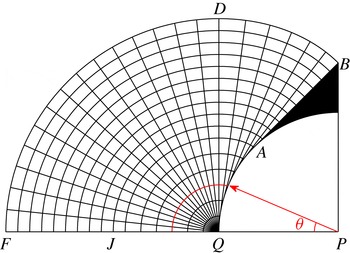
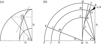
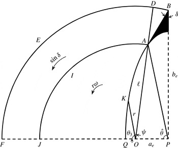
First we review the characteristics field found analytically; see figure 2. Only a quarter of the circular geometry is presented. The following are the main features. The maximum shear will happen on the
 $x$
-axis. Hence the
 $x$
-axis is a straight characteristic,
 $QF$
(say
 $\unicode[STIX]{x1D6FC}$
-line), and thus all the characteristics from the same family will be straight (direct consequence of Hencky equations (see Hill Reference Hill1950)). The shear stress on the
 $y$
-axis is zero. Therefore, the
 $y$
-axis is in the direction of principle stress and the characteristics intersect at an angle
 $\pm \unicode[STIX]{x03C0}/4$
, e.g. like
 $AB$
. The maximum shear occurs on the disc surface. Consequently, the
 $\unicode[STIX]{x1D6FC}$
-lines are tangent to the disc surface, e.g. lines
 $AB$
and
 $QD$
. There is a singular point
 $Q$
, which is the centre of a fan filling the space between the last
 $\unicode[STIX]{x1D6FC}$
-line tangent to the surface (
 $QD$
) and the
 $x$
-axis (
 $QF$
). In figure 2 the dark shaded region shows the plug that is attached to the front of the particle. In this region, both
 $\unicode[STIX]{x1D6FC}$
- and
 $\unicode[STIX]{x1D6FD}$
-lines are straight: a region of constant state. Indeed, Hencky equations dictate that the
 $\unicode[STIX]{x1D6FC}$
-lines are straight for particles with two orthogonal lines of symmetry because the symmetry line of the particle perpendicular to the direction of movement (
 $x$
-axis) is a straight
 $\unicode[STIX]{x1D6FC}$
-line. The velocity field associated with the characteristics is governed by Geiringer equations. We find
 $\tilde{u} _{\unicode[STIX]{x1D6FC}}=0$
and
 $\tilde{u} _{\unicode[STIX]{x1D6FD}}=\text{const}.$
along the
 $\unicode[STIX]{x1D6FD}$
-lines. The velocity boundary condition on the particle surface defines
 $\tilde{u} _{\unicode[STIX]{x1D6FD}}$
. Along the group of
 $\unicode[STIX]{x1D6FD}$
-lines emanating from
 $AB$
,
 $\tilde{u} _{\unicode[STIX]{x1D6FD}}=1/\sqrt{2}$
(note the particle velocity is 1), and for the
 $\unicode[STIX]{x1D6FD}$
-lines emanating from
 $QA$
,
 $\tilde{u} _{\unicode[STIX]{x1D6FD}}=\sin \unicode[STIX]{x1D703}$
, where
 $\unicode[STIX]{x1D703}$
is shown in figure 2.
Characteristic network adjacent to a circle.

Figure 3 plots the shear stress
 $\unicode[STIX]{x1D70F}_{xy}^{\ast }$
computed from the [R] problem at
 $B=10^{4}$
(left) and that from the characteristics analysis
 $\tilde{\unicode[STIX]{x1D70F}}_{xy}$
(right). Both shear stresses have been normalized with
 $B$
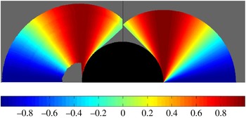
. Firstly, we see that the envelope of the characteristics does not agree fully with the outer yield surface of the viscoplastic computation. Secondly, we see that the shear stresses are different. The characteristics solution has a single rigid plug at the front, whereas the viscoplastic solution also has a second plug along the side of the cylinder. The frontal plugs also differ slightly in size. Figure 4 compares the velocity along the
 $x$
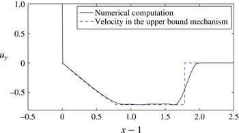
-axis. The perfectly plastic velocity has a discontinuity in the velocity both at the cylinder surface and at the outer characteristic surface. The viscoplastic fluid has no discontinuities. A narrow viscous boundary layer is found close to the cylinder, then a rigid plug, followed by yielding and slow deformation into a (near-)constant downwards velocity, then a further viscous layer at the outside of the flow envelope. Given the disparities in both stress and velocity fields, it is perhaps surprising that the computational comparisons of the limiting plastic drag coefficients in Tokpavi et al. (Reference Tokpavi, Magnin and Jay2008) and Putz & Frigaard (Reference Putz and Frigaard2010) can be so close to the perfectly plastic values.
Normalized shear stresses: left half from computation of the [R] problem with
 $B=10^{4}$
, i.e.
 $\unicode[STIX]{x1D70F}_{xy}^{\ast }/B$
; right half from the characteristics prediction
 $\tilde{\unicode[STIX]{x1D70F}}_{xy}/B$
. Rigid regions are plotted grey.

Computed velocity in the
 $y$
-direction ([R] problem with
 $B=10^{4}$
), measured with distance
 $r$
from the cylinder surface along the
 $x$
-axis.

Further investigation (not shown) reveals that the outer viscous layer does decrease very slowly in width as
 $B\rightarrow \infty$
, as does the sheared zone along the
 $y$
-axis at the front of the particle (also they appear to decrease in width at the same rate with
 $B$
). The equatorial velocities in figure 4 eventually match, although the viscoplastic solutions remain continuous and adopt a boundary layer profile. The rigid plug at the side of the particle in the left part of figure 3 remains as
 $B\rightarrow \infty$
. The reader is referred to Tokpavi et al. (Reference Tokpavi, Magnin and Jay2008) for a detailed quantitative description of such features. It is thus interesting that, although
 $B=10^{4}$
is quite adequate for convergence of the limiting plastic drag coefficients (as we see below), other features of velocity and stress require significantly larger
 $B$
.
3.3 Symmetric particles
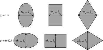
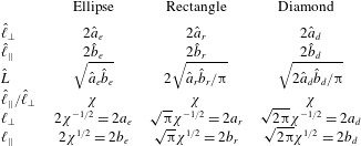
We now examine three other symmetric geometries: ellipse, rectangle and diamond. For each particle geometry,
 $\ell _{\bot }=\hat{\ell }_{\bot }/\hat{L}$
and
 $\ell _{||}=\hat{\ell }_{||}/\hat{L}$
represent the dimensionless lengths of the particle in the
 $x$
- and
 $y$
-directions, respectively. The aspect ratio is always denoted
 $\unicode[STIX]{x1D712}=\ell _{||}/\ell _{\bot }$
and the dimensionless area is
 $\unicode[STIX]{x03C0}$
; see table 1 and figure 5.
Dimensional geometries considered.

Dimensional and dimensionless parameters for the three geometries.

3.3.1 Ellipse
Putz & Frigaard (Reference Putz and Frigaard2010) computed viscoplastic flows around a settling ellipse and approximated the limiting plastic drag coefficient by generalizing the expression of Randolph & Houlsby (Reference Randolph and Houlsby1984) for a circle. However, the proposed approximation was poor for
 $\unicode[STIX]{x1D712}>1$
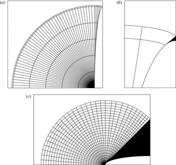
, the main problem being that the characteristic network was not constructed. The characteristic network may be constructed by generalizing the statements made about the circle. Figure 6 shows the characteristics for
 $\unicode[STIX]{x1D712}=10$
and
 $0.2$
. It can be seen that for
 $\unicode[STIX]{x1D712}<1$
the rigid plug at the front is much larger than for
 $\unicode[STIX]{x1D712}>1$
. In the limiting case
 $\unicode[STIX]{x1D712}\rightarrow 0$
the ellipse approaches a thin plate moving in the direction of its thickness and the plug region approaches a right-angled triangle with height equal to the plate half-length.
Characteristic network around an ellipse: (a)
 $\unicode[STIX]{x1D712}=10$
; (b) zoom of frontal plug region for
 $\unicode[STIX]{x1D712}=10$
; (c)
 $\unicode[STIX]{x1D712}=0.2$
.

From the characteristic network we are able to calculate the lower bound of the plastic drag coefficient as follows (see figure 7 for the geometrical parameters).
-
(1) Shear stress contribution on
$AB$
: (3.1)
$$\begin{eqnarray}F_{1-1}=\unicode[STIX]{x1D712}^{-1/2}B\cos \unicode[STIX]{x1D703}_{1}^{\ast }.\end{eqnarray}$$
-
(2) Normal stress contribution on
$AB$
: (3.2)
$$\begin{eqnarray}F_{2-1}=\unicode[STIX]{x1D712}^{-1/2}B\left(\bar{\unicode[STIX]{x1D70E}}+\frac{3\unicode[STIX]{x03C0}}{2}\right)\cos \unicode[STIX]{x1D703}_{1}^{\ast }.\end{eqnarray}$$
-
(3) Shear stress contribution on
$AKSQ$
: (3.3)
$$\begin{eqnarray}F_{3-1}=\int _{0}^{\unicode[STIX]{x1D703}_{1}^{\ast }}B\sin \unicode[STIX]{x1D701}\sqrt{\unicode[STIX]{x1D712}^{-1}\sin ^{2}\unicode[STIX]{x1D703}_{1}+\unicode[STIX]{x1D712}\cos ^{2}\unicode[STIX]{x1D703}_{1}}\,\text{d}\unicode[STIX]{x1D703}_{1}.\end{eqnarray}$$
-
(4) Normal stress contribution on
$AKSQ$
: (3.4)Here
$$\begin{eqnarray}F_{4-1}=\int _{0}^{\unicode[STIX]{x1D703}_{1}^{\ast }}B[\bar{\unicode[STIX]{x1D70E}}+2(\unicode[STIX]{x03C0}-\unicode[STIX]{x1D701})]\cos \unicode[STIX]{x1D701}\sqrt{\unicode[STIX]{x1D712}^{-1}\sin ^{2}\unicode[STIX]{x1D703}_{1}+\unicode[STIX]{x1D712}\cos ^{2}\unicode[STIX]{x1D703}_{1}}\,\text{d}\unicode[STIX]{x1D703}_{1}.\end{eqnarray}$$
$\unicode[STIX]{x1D703}_{1}=\tan ^{-1}(\unicode[STIX]{x1D712}^{-1}\tan \unicode[STIX]{x1D703})$
and
$\unicode[STIX]{x1D703}_{1}^{\ast }=\tan ^{-1}\unicode[STIX]{x1D712}$
. The unknown mean stress through the
$QNJF$
is designated by
$B\bar{\unicode[STIX]{x1D70E}}$
.





Geometrical parameters for lower- and upper-bound calculations.

So far we have calculated the force acting on a quarter of the particle. For the total force, we repeat the same procedure to obtain the forces acting on the three remaining quarters and sum. The terms involving
 $B\bar{\unicode[STIX]{x1D70E}}$
cancel due to symmetry, whereas the other terms are added together. The lower-bound plastic drag coefficient is
 $$\begin{eqnarray}\displaystyle [C_{D,c}^{p}]_{L} & = & \displaystyle \frac{[\tilde{F}^{p}]_{L}}{\ell _{\bot }B}=\frac{\displaystyle \mathop{\sum }_{i=1}^{4}F_{i}}{2\unicode[STIX]{x1D712}^{-1/2}B}\nonumber\\ \displaystyle & = & \displaystyle (2+3\unicode[STIX]{x03C0})\cos \unicode[STIX]{x1D703}_{1}^{\ast }+2\int _{0}^{\unicode[STIX]{x1D703}_{1}^{\ast }}\{\unicode[STIX]{x1D712}\cos \unicode[STIX]{x1D703}_{1}+[\unicode[STIX]{x03C0}+2\cot ^{-1}(\unicode[STIX]{x1D712}\cot \unicode[STIX]{x1D703}_{1})]\sin \unicode[STIX]{x1D703}_{1}\}\,\text{d}\unicode[STIX]{x1D703}_{1},\nonumber\\ \displaystyle & & \displaystyle\end{eqnarray}$$
where
 $F_{i}=\sum _{j=1}^{4}F_{j-i}$
for the
 $i$
th quarter of the circle. We also construct velocity solutions on the characteristic network, which lead to an upper bound for the force and plastic drag coefficient. Two different mechanisms are proposed (see appendix B), the first of which significantly overestimates the plastic drag coefficient at large
 $\unicode[STIX]{x1D712}$
.
We have also computed the limiting viscoplastic solutions, using both [R] and [M] problems, for a wide range of
 $\unicode[STIX]{x1D712}$
. Convergence of the calculation of
 $Y_{c}$
using (2.25) and the solution of the [R] problem at large
 $B$
are illustrated in figure 8 for three different
 $\unicode[STIX]{x1D712}$
: for
 $B\geqslant 10^{4}$
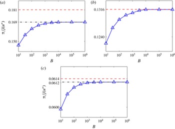
no significant changes in plastic drag coefficient occur but the computations become more difficult. Calculations of
 $Y_{c}$
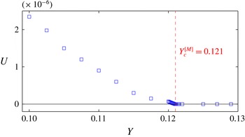
using the [M] problem are direct, but involve iterating on
 $Y$
until the flow stops. The agreement between
 $Y_{c}$
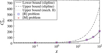
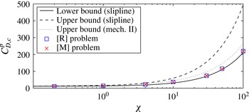
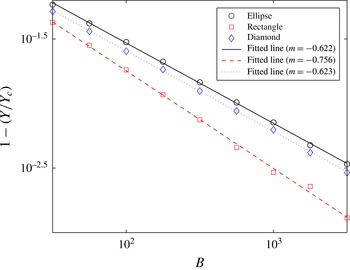
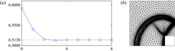
using [R] or [M] is within 1 % for all our results illustrated, and is often better (see appendix C for an example comparison). Figure 9 compares the bounds of the plastic drag coefficient with those obtained numerically from the viscoplastic flow. The [R] problem data are obtained at
 $B=10^{4}$
. Quite good agreement can be observed between the lower-bound plastic solution and the computed coefficients from the viscoplastic problem, although they do not match exactly (except at
 $\unicode[STIX]{x1D712}=1$
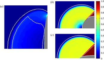
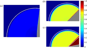
). The upper-bound plastic solutions are less accurate. Some example computations of the viscoplastic flow are shown in figure 10 and other detailed examples are shown in Putz & Frigaard (Reference Putz and Frigaard2010). These show regions of constant speed for
 $\unicode[STIX]{x1D712}\leqslant 1$
and a large rigid plug region at the sides of the particle, for
 $\unicode[STIX]{x1D712}>1$
. The yield surfaces are marked in white.
Dependence of plastic dissipation on the Bingham number for an ellipse: (a)
 $\unicode[STIX]{x1D712}=10$
; (b)
 $\unicode[STIX]{x1D712}=1$
; (c)
 $\unicode[STIX]{x1D712}=0.2$
. The blue triangles are data from the [R] problem. The red dashed lines are the characteristics predictions, and black dot-dashed lines are the asymptotic values of the blue symbols for large Bingham numbers.

Critical plastic drag coefficient of 2D elliptical particles.

Velocity magnitude colour map, computed from problem [R] at
 $B=10^{4}$
(the white lines are the yield surfaces): (a)
 $\unicode[STIX]{x1D712}=10$
, (b)
 $\unicode[STIX]{x1D712}=1$
, (c)
 $\unicode[STIX]{x1D712}=0.2$
.

3.3.2 Rectangle
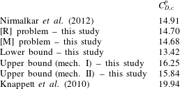
To the best of our knowledge, there is no prior study concerning the characteristic network around a rectangular particle, although Knappett et al. (Reference Knappett, Mohammadi and Griffin2010) estimate an upper bound for the mechanical work dissipated in the plastic region around a square cross-section pile by suggesting a (non-admissible) velocity field. Appendix C presents a comparison of this and other known results for the square, with those computed here.
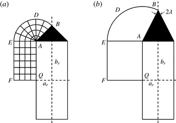
(a) Schematic of characteristic network adjacent to a rectangle, and (b) geometrical parameters for calculation of upper bound.

The characteristic network for the rectangle is illustrated in figure 11. Again, the
 $y$
-axis bisects the right angle at point
 $B$
. The points
 $A$
and
 $Q$
of the ellipse network (e.g. figure 2) have shrunk to the singular point
 $A$
at the corner of the rectangle. Here, again, the
 $x$
-axis would be an
 $\unicode[STIX]{x1D6FC}$
-line. Thus, a region of two orthogonal families of parallel straight lines will be formed (
 $AEFQ$
) along the side of the rectangle. The lower bound for the plastic drag force for this case consists of the following contributions.
-
(1) Shear stress contribution on
$AB$
: (3.6)
$$\begin{eqnarray}F_{1-1}=\sqrt{\unicode[STIX]{x03C0}}\unicode[STIX]{x1D712}^{-1/2}B/2.\end{eqnarray}$$
-
(2) Shear stress contribution on
$AQ$
: (3.7)
$$\begin{eqnarray}F_{2-1}=\sqrt{\unicode[STIX]{x03C0}}\unicode[STIX]{x1D712}^{1/2}B/2.\end{eqnarray}$$
-
(3) Normal stress contribution on
$AB$
: (3.8)
$$\begin{eqnarray}F_{3-1}=\sqrt{\unicode[STIX]{x03C0}}\unicode[STIX]{x1D712}^{-1/2}B\left.\left(\bar{\unicode[STIX]{x1D70E}}+\frac{3\unicode[STIX]{x03C0}}{2}\right)\right/2.\end{eqnarray}$$


Summing over four quarters of the rectangle (cancelling the mean normal stress contributions
 $\bar{\unicode[STIX]{x1D70E}}$
and noting
 $\ell _{\bot }=\sqrt{\unicode[STIX]{x03C0}/\unicode[STIX]{x1D712}}$
) leads us to
 $$\begin{eqnarray}\left[C_{D,c}^{p}\right]_{L}=\frac{\left[\tilde{F}^{p}\right]_{L}}{\ell _{\bot }B}=2+3\unicode[STIX]{x03C0}+2\unicode[STIX]{x1D712}.\end{eqnarray}$$
We may also calculate an upper bound for the plastic drag coefficient based on the general mechanism illustrated in figure 11(b). This mechanism is defined by a single geometrical optimization parameter,
 $\unicode[STIX]{x1D706}$
. The upper bound based on the characteristic network then can simply be obtained by setting
 $\unicode[STIX]{x1D706}=\unicode[STIX]{x03C0}/4$
.
-
(1) Velocity discontinuity on line
$AB$
: (3.10)
$$\begin{eqnarray}\unicode[STIX]{x0394}W_{1}=\sqrt{\unicode[STIX]{x03C0}}\unicode[STIX]{x1D712}^{-1/2}/2B\cot \unicode[STIX]{x1D706}.\end{eqnarray}$$
-
(2) Velocity discontinuity on line
$BDE$
: (3.11)
$$\begin{eqnarray}\unicode[STIX]{x0394}W_{2}=\left.\sqrt{\unicode[STIX]{x03C0}}\unicode[STIX]{x1D712}^{-1/2}\right/2B\left(\frac{\unicode[STIX]{x03C0}}{2}+\unicode[STIX]{x1D706}\right).\end{eqnarray}$$
-
(3) Work dissipation in area
$BDEA$
: (3.12)
$$\begin{eqnarray}\unicode[STIX]{x0394}W_{3}=\left.\sqrt{\unicode[STIX]{x03C0}}\unicode[STIX]{x1D712}^{-1/2}\right/2B\left(\frac{\unicode[STIX]{x03C0}}{2}+\unicode[STIX]{x1D706}\right).\end{eqnarray}$$
-
(4) Velocity discontinuity on line
$EF$
: (3.13)
$$\begin{eqnarray}\unicode[STIX]{x0394}W_{4}=\sqrt{\unicode[STIX]{x03C0}}\unicode[STIX]{x1D712}^{1/2}/2B\sin \unicode[STIX]{x1D706}.\end{eqnarray}$$
-
(5) Velocity discontinuity on line
$AQ$
: (3.14)
$$\begin{eqnarray}\unicode[STIX]{x0394}W_{5}=\sqrt{\unicode[STIX]{x03C0}}\unicode[STIX]{x1D712}^{1/2}/2B\left(1+\sin \unicode[STIX]{x1D706}\right).\end{eqnarray}$$


The upper bound is obtained by repeating and summing over the four quarters of the domain:
 $$\begin{eqnarray}[C_{D,c}^{p}]_{U}=2\cot \unicode[STIX]{x1D706}+(2\unicode[STIX]{x03C0}+4\unicode[STIX]{x1D706})+\unicode[STIX]{x1D712}(2+4\sin \unicode[STIX]{x1D706}).\end{eqnarray}$$
As can be observed, the upper bound associated with the characteristic network (
 $\unicode[STIX]{x1D706}=\unicode[STIX]{x03C0}/4$
) will converge to the lower bound as
 $\unicode[STIX]{x1D712}\rightarrow 0$
, but has a large discrepancy as
 $\unicode[STIX]{x1D712}\rightarrow \infty$
(i.e.
 $[C_{D,c}^{p}]_{U}-[C_{D,c}^{p}]_{L}=2\sqrt{2}\unicode[STIX]{x1D712}$
). In principle, this discrepancy can be reduced for large
 $\unicode[STIX]{x1D712}$
by selecting
 $\unicode[STIX]{x1D706}$
optimally. The result of this alternative velocity field is represented as mechanism II in figure 12.
We have also calculated the limiting viscoplastic solutions, using both problems [M] and [R] (again at
 $B=10^{4}$
). The computed
 $C_{D,c}^{p}$
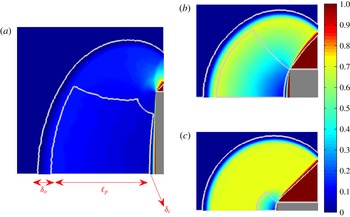
are again close to the perfect plasticity lower bound; see figure 12. Some example computations of the velocity magnitude colour maps and the yield surfaces are shown in figure 13. The
 $\unicode[STIX]{x03C0}/4$
angle between the yield surface of the attached plug and the direction of motion is clearly visible. Despite the good agreement with the limiting drag coefficients, we observe a very noticeable difference between the shape of the outer yield surface and the outermost
 $\unicode[STIX]{x1D6FD}$
-line in the plastic solutions; see figure 11(a). This is particularly evident in the case of large
 $\unicode[STIX]{x1D712}$
. The boundary layer between the particle and the plug appears to elongate with large
 $\unicode[STIX]{x1D712}$
, extending along the sides of the rectangle. We explore this boundary layer and the limiting flows further in § 4.3.
Critical plastic drag coefficients for a rectangular particle.

Velocity magnitude colour map, computed from problem [R] at
 $B=10^{4}$
(the white lines are the yield surfaces): (a)
 $\unicode[STIX]{x1D712}=10$
; (b)
 $\unicode[STIX]{x1D712}=1$
; (c)
 $\unicode[STIX]{x1D712}=0.2$
.

3.3.3 Diamond
The diamond-shaped particle is interesting chiefly because of the behaviour of the plug attached to the front of the particle. For
 $\unicode[STIX]{x1D712}<1$
the attached plug extends in front of (and behind) the entire diamond, to form an angle
 $\unicode[STIX]{x03C0}/4$
with the
 $y$
-axis, so that the particle and plug together form a square rotated by
 $\unicode[STIX]{x03C0}/4$
. However, the story is different for
 $\unicode[STIX]{x1D712}\geqslant 1$
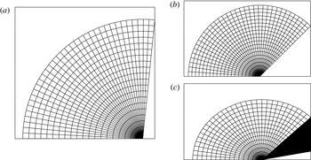
: no attached frontal plug region will be formed. Instead, two centred fans, with radius equal to the length of the side, cover the entire plastic region. Figure 14 shows the characteristic network for three diamonds with different aspect ratios
 $\unicode[STIX]{x1D712}$
.
Characteristic network around the diamond: (a)
 $\unicode[STIX]{x1D712}=10$
; (b)
 $\unicode[STIX]{x1D712}=1$
; (c)
 $\unicode[STIX]{x1D712}=0.2$
.

The lower and upper bounds of the plastic drag force can now be determined easily by re-examining the terms associated with the centred fan in the characteristic network of the rectangle. The most interesting point is that the upper and lower bounds (calculated based on the characteristic network) are identical for this case, which means that the calculated plastic drag force (and coefficient) is exact:
 $$\begin{eqnarray}C_{D,c}^{p}=\left\{\begin{array}{@{}ll@{}}2\unicode[STIX]{x1D712}+4(\unicode[STIX]{x03C0}-\tan ^{-1}\unicode[STIX]{x1D712})\quad & \text{for }\unicode[STIX]{x1D712}\geqslant 1,\\ 2+3\unicode[STIX]{x03C0}\quad & \text{for }\unicode[STIX]{x1D712}<1.\end{array}\right.\end{eqnarray}$$
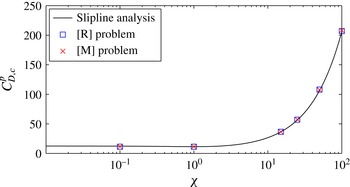
This result has been known for some time in the plasticity community, e.g. derived also by Poulos & Davis (Reference Poulos and Davis1980), who examined the effect of aspect ratio on the lateral resistance of a rough pile (with rhombus cross-section). Figure 15 compares (3.16) with the limiting plastic drag coefficient computed from the viscoplastic problem, showing very good agreement. Figure 16 presents three example computations for the diamond-shaped particle. The outer yield surfaces in both the characteristics analysis and the computed viscoplastic solution are very similar. The excellent agreement is largely due to there being no ‘side’ region to the particle. In the case of the ellipse and rectangle (at large
 $\unicode[STIX]{x1D712}$
), the tip and sides of the particle are different, with a boundary layer emerging along the sides. The diamond has only a long tip.
Critical plastic drag coefficient of diamond.

Velocity magnitude contours around the diamond: (a)
 $\unicode[STIX]{x1D712}=10$
; (b)
 $\unicode[STIX]{x1D712}=1$
; (c)
 $\unicode[STIX]{x1D712}=0.2$
.

3.4 Summary
So far we have seen that the lower-bound perfectly plastic solutions appear to give a very reasonable approximation to the limiting plastic drag coefficients computed for the viscoplastic problem. This is both interesting and in some sense remarkable. Although there are cases for which the solutions are very close or exact, e.g. the diamond, other cases such as the rectangle have completely different yielded envelopes around the particle. Intermediate cases such as the ellipse contain special geometries (the circle) for which plastic and viscoplastic solutions agree, although the stress fields are not totally the same.
The upper-bound plastic velocity fields are much less effective as estimates for the limiting viscoplastic solutions. One reason for this is that the plastic test functions may be discontinuous whereas the viscoplastic solutions vary continuously due to viscous effects, albeit often approaching discontinuity in thin boundary layers. In many cases the transition occurs in (relatively) thin layers of (relatively) high strain rate, which contribute significantly to the plastic dissipation in the limit of zero flow. The other difference in the upper-bound velocity fields is that the boundary conditions on the tangential component are not specified at a solid surface.
4 General features of limiting viscoplastic solutions
In the previous section we have presented computations of three different geometric families of particles, at various aspect ratios, close to the static limit. We have compared these with estimates from perfectly plastic upper and lower bounds. First, in understanding the generic behaviour of this yielding process, two geometric trends are apparent: (i) as
 $\unicode[STIX]{x1D712}\rightarrow 0$
the flow geometries all appear very similar; and (ii) for large
 $\unicode[STIX]{x1D712}$
we generate boundary layers in the static limit and there seems to be some degree of commonality between different geometries. We explore these limits below. The second observation is that, although perfectly plastic flows may on occasion predict the limit
 $Y_{c}$
accurately, they contain no information on the convergence behaviour (with
 $B$
or
 $Y_{c}^{-}-Y$
). Perfectly plastic flow solutions contain
 $B$
only as a scaling parameter: the stress and velocity fields otherwise depend only on the particle shape, i.e.
 $\unicode[STIX]{x1D712}$
in each geometry. Thus, here we concentrate on the viscoplastic solutions.
4.1 The limit
$\unicode[STIX]{x1D712}\rightarrow 0$

The limit
 $\unicode[STIX]{x1D712}\rightarrow 0$
gives the greatest agreement between drag coefficients computed from the viscoplastic flow and the characteristics analysis. The structure of the solution that we have seen in our viscoplastic computations consists of (up to) five regions as
 $\unicode[STIX]{x1D712}\rightarrow 0$
. Referring to one quarter of the flow domain, these regions are as follows.
-
(i) A rigid plug attached to the front (and rear) of the particle, of width
${\sim}\ell _{\bot }/2$
as
$\unicode[STIX]{x1D712}\rightarrow 0$
, and forming a triangular region fore–aft of the particle, making an angle
$\unicode[STIX]{x03C0}/4$
with the
$y$
-axis. -
(ii) A rotating zone that is centred at the ‘corner’ of the rigid plug, where it contacts the particle. The fluid rotates on circular streamlines about this point and appears to have approximately constant speed in the azimuthal direction. The radius of this region is
${\sim}\ell _{\bot }/\sqrt{2}$
and the azimuthal speed is
${\sim}1/\sqrt{2}$
. -
(iii) A thin shear layer between the attached rigid plug and the rotating zone. The length of this boundary layer is
$\ell _{\bot }/\sqrt{2}$
. Across the layer the normal component of velocity is continuous and the tangential drop from
$1/\sqrt{2}$
to
$0$
. -
(iv) An outer boundary layer, surrounding the rotating zone, across which the azimuthal velocity drops from
$1/\sqrt{2}$
to
$0$
. The circumferential length of this boundary layer is
$3\unicode[STIX]{x03C0}\ell _{\bot }/(4\sqrt{2})$
. We have not studied the thickness, but it does not appear to grow as
$\unicode[STIX]{x1D712}\rightarrow 0$
. -
(v) A ‘side region’ that connects the rotating regions fore and aft. This region has width
${\sim}\ell _{\bot }/2$
and height
${\sim}\unicode[STIX]{x1D712}\ell _{||}$
(ellipse) or
${\sim}\ell _{||}$
(rectangle). This region is absent in the case of the diamond shape.


We can estimate the contributions to
 $j(\boldsymbol{u}^{\ast })$
from each of the above regions as follows: (i)
 $0$
; (ii)
 ${\sim}3\unicode[STIX]{x03C0}\ell _{\bot }/2$
; (iii)
 ${\sim}2\ell _{\bot }$
; (iv)
 ${\sim}3\unicode[STIX]{x03C0}\ell _{\bot }/2$
; (v)
 ${\sim}\unicode[STIX]{x1D712}\ell _{||}/2$
(ellipse) or
 ${\sim}\ell _{||}/2$
(rectangle). Combining these we find:
 $C_{D,c}^{p}=\lim _{B\rightarrow \infty }[j(\boldsymbol{u}^{\ast })/\ell _{\bot }]\sim 2+3\unicode[STIX]{x03C0}$
, for all three geometries as
 $\unicode[STIX]{x1D712}\rightarrow 0$
, which agrees with the characteristics estimates at leading order.
In order to estimate convergence with respect to
 $\unicode[STIX]{x1D712}$
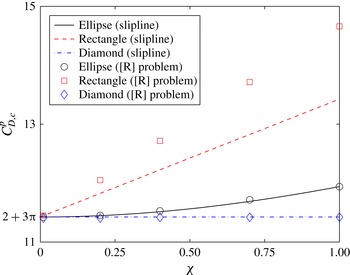
, we would need to know the next order of terms in each of the above regions, which is not apparent. Figure 17 plots the critical plastic drag coefficient for different
 $\unicode[STIX]{x1D712}$
, as
 $\unicode[STIX]{x1D712}\rightarrow 0$
, computed with
 $B=10^{4}$
. It is rather interesting that the diamond shape shows no variation with
 $\unicode[STIX]{x1D712}$
for
 $\unicode[STIX]{x1D712}<1$
. As the diamond has no ‘sides’ and only the tip region, the main role of
 $\unicode[STIX]{x1D712}$
is to determine the width of the particle, from which we have seen there results an attached fore–aft plug. The unyielded plug is thus indistinguishable from the particle and we see no variation with
 $\unicode[STIX]{x1D712}$
.
Critical plastic drag coefficient for
 $\unicode[STIX]{x1D712}\rightarrow 0$
, computed with
 $B=10^{4}$
.

By the same analogy, the parts of the ellipse and rectangle that lie within the fore–aft angular plug regions as
 $\unicode[STIX]{x1D712}\rightarrow 0$
should not have any influence on the flow convergence with
 $\unicode[STIX]{x1D712}$
. This suggests that
 $\unicode[STIX]{x1D712}$
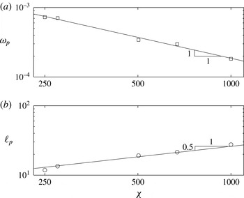
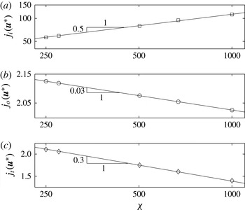
dependence comes only from the side region, denoted (v) above. For the ellipse the surface tangent that is at
 $\unicode[STIX]{x03C0}/4$
to the
 $y$
-axis meets the surface at
 $$\begin{eqnarray}\displaystyle y=\frac{\ell _{||}}{2}\sqrt{\frac{\unicode[STIX]{x1D712}^{2}}{1+\unicode[STIX]{x1D712}^{2}}}\sim \frac{\unicode[STIX]{x1D712}\ell _{||}}{2}. & & \displaystyle\end{eqnarray}$$
The contribution from this side region to
 $j(\boldsymbol{u}^{\ast })$
is thus
 ${\sim}\unicode[STIX]{x1D712}\ell _{||}$
and to
 $C_{D,c}^{p}$
is
 ${\sim}\unicode[STIX]{x1D712}\ell _{||}/\ell _{\bot }\sim \unicode[STIX]{x1D712}^{2}$
. For the rectangle, we have instead that the contribution to
 $C_{D,c}^{p}$
is
 ${\sim}\ell _{||}/\ell _{\bot }\sim \unicode[STIX]{x1D712}$
. We see that these estimates do agree with the (approximately) quadratic and linear variations in figure 17, for ellipse and rectangle, respectively.
Regarding
 $B$
dependence, generally this must be examined numerically. However, for the diamond we may progress via a rescaling argument as follows. Defining
 $\check{\boldsymbol{x}}=2\boldsymbol{x}/\ell _{\bot }$
we rescale the lengths while keeping velocities unchanged in problem [R]. If we also rescale
 $\check{\unicode[STIX]{x1D70F}}_{ij}^{\ast }=(\ell _{\bot }/2)\unicode[STIX]{x1D70F}_{ij}^{\ast }$
and
 $\check{p}^{\ast }=(\ell _{\bot }/2)p^{\ast }$
, the Stokes equations are satisfied by the rescaled stress tensor, which is characterized by a single parameter,
 $$\begin{eqnarray}\check{B}=\frac{\ell _{\bot }}{2}B.\end{eqnarray}$$
The re-mapped diamond intersects the
 $\check{x}$
-axis at
 $\pm 1$
and the
 $\check{y}$
-axis at
 $\pm \unicode[STIX]{x1D712}$
. For any fixed
 $\unicode[STIX]{x1D712}<1$
the limit
 $B\rightarrow \infty$
is the same as
 $\check{B}\rightarrow \infty$
.
We have already seen that as
 $\check{B}\rightarrow \infty$
the solution will have a rigid plug attached to the diamond that intersects the
 $\check{y}$
-axis at
 $\pm 1$
, and then regions (ii)–(iv), as described above. The contributions to
 $j(\check{\boldsymbol{u}}^{\ast })$
from regions (ii)–(iv) are
 $3\unicode[STIX]{x03C0}$
,
 $4$
and
 $3\unicode[STIX]{x03C0}$
, respectively. However, since now
 $\check{\boldsymbol{u}}^{\ast }$
depends only on
 $\check{B}$
, we may postulate convergence,
 $$\begin{eqnarray}j(\check{\boldsymbol{u}}^{\ast })\sim 4+6\unicode[STIX]{x03C0}+2A\check{B}^{-t}\quad \text{as}~\check{B}\rightarrow \infty ,\end{eqnarray}$$
for constants
 $A$
and
 $t>0$
. On rescaling lengths,
 $j(\boldsymbol{u}^{\ast })=(\ell _{\bot }/2)j(\check{\boldsymbol{u}}^{\ast })\sim \ell _{\bot }(2+3\unicode[STIX]{x03C0}+A\check{B}^{-t}),~\text{as}~\check{B}\rightarrow \infty$
. From this we deduce that
 $$\begin{eqnarray}C_{D,c}^{p}=\lim _{B\rightarrow \infty }\frac{j(\boldsymbol{u}^{\ast })}{\ell _{\bot }}\sim 2+3\unicode[STIX]{x03C0}+O(B^{-t}).\end{eqnarray}$$
The exponent
 $t$
can be deduced economically from computation of
 $\check{\boldsymbol{u}}^{\ast }$
as
 $\check{B}\rightarrow \infty$
. We have found
 $t\approx 0.70$
from fitting a power-law expression to our data.
4.2 A general framework
We would like to understand the limit
 $Y\rightarrow Y_{c}^{-}$
. The rescaling leading to (2.24) clarifies that
 $Y\rightarrow Y_{c}^{-}$
and
 $B\rightarrow \infty$
are the same limit, but does not actually determine the relationship between the two parameters. As well as clarifying this relationship, we would like to be able to determine the decay rates. The only general results we have are the decay bounds (2.20) and (2.21) for problem [M], as
 $Y\rightarrow Y_{c}^{-}$
.
To this end, let us suppose that the particle velocity
 $U\sim b(\unicode[STIX]{x1D712})(1-Y/Y_{c})^{\unicode[STIX]{x1D708}}$
, for some positive exponent
 $\unicode[STIX]{x1D708}=\unicode[STIX]{x1D708}(\unicode[STIX]{x1D712})$
. The bound (2.20) implies that
 $\unicode[STIX]{x1D708}\geqslant 1$
and (2.22) gives us
 $j(\boldsymbol{u})\sim b(\unicode[STIX]{x1D712})(1-Y/Y_{c})^{\unicode[STIX]{x1D708}}\unicode[STIX]{x03C0}/Y_{c}$
. The rescaling of (2.24) then tells us that
 $$\begin{eqnarray}B=\frac{Y}{U}\sim \frac{Y_{c}(\unicode[STIX]{x1D712})}{b(\unicode[STIX]{x1D712})}(1-Y/Y_{c})^{-\unicode[STIX]{x1D708}},\end{eqnarray}$$
which couples the limits
 $Y\rightarrow Y_{c}^{-}$
and
 $B\rightarrow \infty$
. To find
 $\unicode[STIX]{x1D708}$
we must estimate the limiting solutions.
Suppose we compute problem [R] at large
 $B$
and substitute the velocity
 $\boldsymbol{u}^{\ast }$
into (2.25), i.e. we approximate
 $Y_{c}$
using the limiting values of
 $j(\boldsymbol{u}^{\ast })$
. If the contributions to
 $j(\boldsymbol{u}^{\ast })$
come from the entire flow domain, it seems clear that determination of
 $\unicode[STIX]{x1D708}$
is best carried out numerically. This occurs primarily for
 $\unicode[STIX]{x1D712}\sim O(1)$
. The best-studied example is the circular disc. Looking back at figure 4 it becomes evident that
 $j(\boldsymbol{u}^{\ast })$
will have contributions from at least three regions: the boundary layer close to the particle, the outer shear layer, and the zone of near-constant azimuthal velocity. The plug region converges to a fixed size as
 $B\rightarrow \infty$
(Tokpavi et al.
Reference Tokpavi, Magnin and Jay2008), and so each of these regions continues to contribute at leading order. Tokpavi et al. (Reference Tokpavi, Magnin and Jay2008) find that the boundary layer thickness between the small rigid plug on the disc equator and the particle scales like
 $B^{-0.52}$
and the convergence of their plastic drag coefficient to its limiting value scales like
 $B^{-0.55}$
(i.e.
 $\unicode[STIX]{x1D708}\approx 1.82$
). Our results (see figure 8
b) also have
 $\unicode[STIX]{x1D708}\approx 2$
, consistent with Tokpavi et al. (Reference Tokpavi, Magnin and Jay2008). Putz & Frigaard (Reference Putz and Frigaard2010) calculate the limiting exponents for elliptical particles at
 $\unicode[STIX]{x1D712}=0.5$
, 1 and 2, as
 $\unicode[STIX]{x1D708}=1.37\pm 0.23$
,
 $1.20\pm 0.26$
and
 $1.84\pm 0.25$
, respectively. The convergence rate for
 $\unicode[STIX]{x1D712}=1$
does not agree with our present computations, nor with those of Tokpavi et al. (Reference Tokpavi, Magnin and Jay2008), although the values for
 $\unicode[STIX]{x1D708}=0.5$
and
 $2$
are consistent with our calculations. Evidently, calculating each such
 $\unicode[STIX]{x1D712}\sim O(1)$
geometry is laborious. The small-
 $\unicode[STIX]{x1D712}$
limit offers some simplification. The procedure outlined for the diamond, leading to the estimate
 $\unicode[STIX]{x1D708}\approx 1.43$
for all
 $\unicode[STIX]{x1D712}<1$
(
 $t\approx 0.70$
), should also be applicable to the rectangle and ellipse for sufficiently small
 $\unicode[STIX]{x1D712}$
(as the side regions vanish). Large
 $\unicode[STIX]{x1D712}$
also potentially allows for simplification (see § 4.3 below).
Lastly, note that the separation of geometric dependence from the decay in the solution as
 $Y\rightarrow Y_{c}^{-}$
, leading to (4.5), is justified by numerous examples. Classical 1D flows such as Poiseuille flow (pipe or planar) have
 $\unicode[STIX]{x1D708}=2$
. This also seems to be the case for more complex flows along uniform ducts; for example, Frigaard & Scherzer (Reference Frigaard and Scherzer2000) find
 $\unicode[STIX]{x1D708}=2$
for buoyancy-driven two-fluid exchange flows in circular pipes, with either concentric or stratified interfaces. These flows all have a single shear stress active along the bounding surface or at an interface, which seems to lead to
 $\unicode[STIX]{x1D708}=2$
. For 2D flows along uneven channels, Roustaei et al. (Reference Roustaei, Chevalier, Talon and Frigaard2016) find both
 $\unicode[STIX]{x1D708}\approx 2$
and
 $\unicode[STIX]{x1D708}\approx 1.5$
, depending on the channel shape, with the latter relating to limiting flows with an extensional stress component.
4.3 Long particles
The only way in which we might make general deductions about the limit
 $Y\rightarrow Y_{c}^{-}$
is if the viscoplastic solutions develop distinct geometric forms, in which predictable regions of the flow make the dominant contribution to
 $j(\boldsymbol{u}^{\ast })$
. This might be true in the case of boundary layers, which occur in at least two situations. Firstly, for the ellipse and rectangle at large
 $\unicode[STIX]{x1D712}$
, we have seen that there is a sharp transition from the particle velocity to the velocity of the large plug regions along the sides of the particle, that are in rigid rotation. Secondly, for the diamond the particle transitions into a fan-like structure over a relatively thin layer; see figure 16(a). We consider these two cases below. Note that in both cases the length of the boundary layer is expected to scale with
 $\ell _{||}$
.
4.3.1 Ellipse and rectangle
At large
 $\unicode[STIX]{x1D712}$
, the general solution structure is as illustrated in figure 13(a). Along the sides of the particle there is an inner boundary layer (width
 $\unicode[STIX]{x1D6FF}_{i}$
), then the rigid plug and finally an outer boundary layer (width
 $\unicode[STIX]{x1D6FF}_{o}$
). The rigid plug has width
 $\ell _{p}$
and rotates with angular velocity
 $\unicode[STIX]{x1D714}_{p}$
. While the rigid plug does not contribute to
 $j(\boldsymbol{u}^{\ast })$
, the outer boundary layer does. Equally, there is another contribution from near the tip of the particle, where the fluid pushed out from in front of the plug and dragged upwards in the boundary layer turns and moves back downwards into the plug and outer boundary layer. Thus, we may write
 $j(\boldsymbol{u}^{\ast })=j_{i}(\boldsymbol{u}^{\ast })+j_{o}(\boldsymbol{u}^{\ast })+j_{t}(\boldsymbol{u}^{\ast })$
, denoting the contributions from the three regions.
Writing
 $\boldsymbol{u}^{\ast }=(u^{\ast },v^{\ast })$
, we may evaluate the no-flux condition (2.9) along the
 $x$
-axis for problem [R]:
 $$\begin{eqnarray}\displaystyle 0 & = & \displaystyle \frac{\ell _{\bot }}{2}+\int _{\ell _{\bot }/2}^{\ell _{\bot }/2+\unicode[STIX]{x1D6FF}_{i}}v^{\ast }(x,0)\,\text{d}x+\int _{\ell _{\bot }/2+\unicode[STIX]{x1D6FF}_{i}}^{\ell _{\bot }/2+\unicode[STIX]{x1D6FF}_{i}+\ell _{p}}v^{\ast }(x,0)\,\text{d}x+\int _{\ell _{\bot }/2+\unicode[STIX]{x1D6FF}_{i}+\ell _{p}}^{\ell _{\bot }/2+\unicode[STIX]{x1D6FF}_{i}+\ell _{p}+\unicode[STIX]{x1D6FF}_{o}}v^{\ast }(x,0)\,\text{d}x\nonumber\\ \displaystyle & = & \displaystyle O(\unicode[STIX]{x1D712}^{-1/2})+O(\unicode[STIX]{x1D6FF}_{i})-O(\unicode[STIX]{x1D714}_{p}\ell _{p}^{2})-O(\unicode[STIX]{x1D714}_{p}\ell _{p}\unicode[STIX]{x1D6FF}_{o}).\end{eqnarray}$$
In the limit of
 $\unicode[STIX]{x1D712}\rightarrow \infty$
, our computations of the viscoplastic solution suggest that
 $\unicode[STIX]{x1D714}_{p}\sim \unicode[STIX]{x1D712}^{-1}$
and
 $\ell _{p}\sim \unicode[STIX]{x1D712}^{1/2}$
(see figure 18). This suggests that, as
 $\unicode[STIX]{x1D712}\rightarrow \infty$
, the second and third terms on the right-hand side should balance:
 $\unicode[STIX]{x1D6FF}_{i}\sim O(1)$
. To leading order, the mass flux in the yielded boundary layer dragged upwards by the plate will turn back within the tip region into the rigidly rotating plug.
Geometric behaviour at large
 $\unicode[STIX]{x1D712}$
, computed for the rectangular particle at
 $B=10^{4}$
using problem [R]: (a)
 $\unicode[STIX]{x1D714}_{p}$
; (b)
 $\ell _{p}$
(symbols from computation and solid lines fitted, with the indicated slopes).

We may also evaluate
 $j_{i}(\boldsymbol{u}^{\ast })$
,
 $j_{o}(\boldsymbol{u}^{\ast })$
and
 $j_{t}(\boldsymbol{u}^{\ast })$
directly. Figure 19 presents the variation in these contributions at large
 $\unicode[STIX]{x1D712}$
, evaluated numerically at
 $B=10^{4}$
using problem [R]. The inner boundary layer contribution
 $j_{i}(\boldsymbol{u}^{\ast })\sim \unicode[STIX]{x1D712}^{0.5}$
is clearly dominant. The outer boundary layer contribution
 $j_{o}(\boldsymbol{u}^{\ast })$
is approximately constant and the dissipation in the tip region decays as
 $j_{t}(\boldsymbol{u}^{\ast })\sim \unicode[STIX]{x1D712}^{-0.3}$
.
Contributions to the plastic dissipation at large
 $\unicode[STIX]{x1D712}$
, computed for the rectangular particle at
 $B=10^{4}$
using problem [R]: (a)
 $j_{i}(\boldsymbol{u}^{\ast })$
; (b)
 $j_{o}(\boldsymbol{u}^{\ast })$
; (c)
 $j_{t}(\boldsymbol{u}^{\ast })$
(symbols from computation and solid lines fitted, with the indicated slopes).

We now consider fixed large
 $\unicode[STIX]{x1D712}$
and variations with
 $(1-Y/Y_{c})$
(equivalently
 $B$
), starting with the inner boundary layer. The velocity
 $\boldsymbol{u}^{\ast }$
decays from
 ${\sim}1$
to
 ${\sim}O(1-Y/Y_{c})$
across the width
 $\unicode[STIX]{x1D6FF}_{i}$
and has a length
 ${\sim}\ell _{||}$
along the particle. It follows that the contribution to
 $j(\boldsymbol{u}^{\ast })$
is
 ${\sim}\ell _{||}$
. This must be compatible with problem [M]. On rescaling of
 $\boldsymbol{u}^{\ast }$
we find
 $$\begin{eqnarray}\unicode[STIX]{x03C0}\frac{b(\unicode[STIX]{x1D712})}{Y_{c}(\unicode[STIX]{x1D712})}(1-Y/Y_{c})^{\unicode[STIX]{x1D708}}\sim j(\boldsymbol{u})=Uj(\boldsymbol{u}^{\ast })\sim b(\unicode[STIX]{x1D712})\ell _{||}(1-Y/Y_{c})^{\unicode[STIX]{x1D708}},\end{eqnarray}$$
suggesting that
 $Y_{c}(\unicode[STIX]{x1D712})\sim 1/\ell _{||}\sim \unicode[STIX]{x1D712}^{-1/2}$
. We might explicitly take the leading-order term as corresponding to the drop in velocity along the full length of the particle,
 $$\begin{eqnarray}j(\boldsymbol{u}^{\ast })\sim j_{i}(\boldsymbol{u}^{\ast })\sim 2\ell _{||}+O(\unicode[STIX]{x1D712}^{-1/2})+O(1-Y/Y_{c}),\end{eqnarray}$$
accounting for geometric effects and small non-zero velocity at the edge of the boundary layer. This results explicitly in
 $Y_{c}(\unicode[STIX]{x1D712})\sim \unicode[STIX]{x03C0}/(2\ell _{||})$
at leading order.
This asymptotic behaviour is entirely compatible with our earlier results. The critical plastic drag coefficient is
 $$\begin{eqnarray}C_{D,c}^{p}=\frac{\unicode[STIX]{x03C0}}{\ell _{\bot }Y_{c}}=\lim _{B\rightarrow \infty }\frac{j(\boldsymbol{u}^{\ast })}{\ell _{\bot }}.\end{eqnarray}$$
In every example computed (and those estimated from the lower-bound characteristics solutions) we have
 $C_{D,c}^{p}\sim 2\unicode[STIX]{x1D712}$
at large
 $\unicode[STIX]{x1D712}$
. This coincides precisely with the leading-order contribution
 $j(\boldsymbol{u}^{\ast })\sim 2\ell _{||}$
and with
 $Y_{c}(\unicode[STIX]{x1D712})\sim \unicode[STIX]{x03C0}/(2\ell _{||})$
.
The boundary layer contribution to the viscous dissipation
 $a(\boldsymbol{u}^{\ast },\boldsymbol{u}^{\ast })$
is
 ${\sim}\ell _{||}/\unicode[STIX]{x1D6FF}_{i}$
, which translates to
 $$\begin{eqnarray}a(\boldsymbol{u},\boldsymbol{u})=U^{2}a(\boldsymbol{u}^{\ast },\boldsymbol{u}^{\ast })\sim b^{2}(\unicode[STIX]{x1D712})\ell _{||}\frac{(1-Y/Y_{c})^{2\unicode[STIX]{x1D708}}}{\unicode[STIX]{x1D6FF}_{i}}.\end{eqnarray}$$
Our analysis of (4.6) suggests that
 $\unicode[STIX]{x1D6FF}_{i}\sim (1-Y/Y_{c})^{k}$
, as
 $\unicode[STIX]{x1D712}\rightarrow \infty$
. The bound (2.20) implies
 $k\leqslant 2(\unicode[STIX]{x1D708}-1)$
, whereas (2.21) is more restrictive, implying
 $k\leqslant \unicode[STIX]{x1D708}-1$
(note also
 $\unicode[STIX]{x1D708}\geqslant 1$
). For the narrowest possible boundary layer
 $k=\unicode[STIX]{x1D708}-1$
and for the widest possible
 $k=0$
. However, numerical evidence is that
 $k>0$
. In terms of
 $B$
we have
 $\unicode[STIX]{x1D6FF}_{i}\sim (Y_{c}/b)^{k/\unicode[STIX]{x1D708}}B^{-k/\unicode[STIX]{x1D708}}$
. As we have determined that
 $\unicode[STIX]{x1D6FF}_{i}$
is independent of
 $\unicode[STIX]{x1D712}$
as
 $\unicode[STIX]{x1D712}\rightarrow \infty$
we deduce that
 $$\begin{eqnarray}b(\unicode[STIX]{x1D712})\sim Y_{c}(\unicode[STIX]{x1D712})\sim \unicode[STIX]{x1D712}^{-1/2},\quad \text{as}~\unicode[STIX]{x1D712}\rightarrow \infty .\end{eqnarray}$$
We may then deduce that
 $$\begin{eqnarray}\displaystyle & \displaystyle j(\boldsymbol{u})\sim \frac{\ell _{||}Y_{c}}{B}\sim B^{-1}, & \displaystyle\end{eqnarray}$$
 $$\begin{eqnarray}\displaystyle & \displaystyle a(\boldsymbol{u},\boldsymbol{u})\sim \frac{\ell _{||}Y_{c}^{1/\unicode[STIX]{x1D708}}}{b^{1/\unicode[STIX]{x1D708}-2}}B^{-2+k/\unicode[STIX]{x1D708}}\sim \unicode[STIX]{x1D712}^{-1/2}B^{-2+k/\unicode[STIX]{x1D708}}, & \displaystyle\end{eqnarray}$$
 $$\begin{eqnarray}\displaystyle & \displaystyle B\sim (1-Y/Y_{c})^{-\unicode[STIX]{x1D708}}. & \displaystyle\end{eqnarray}$$
 $\unicode[STIX]{x1D708}$
calculated by fitting our computations, all at
 $\unicode[STIX]{x1D712}=100$
, for the three geometries. We observe different convergence rates
 $\unicode[STIX]{x1D708}$
, with the smaller exponents coming from the rectangle.
So far this is non-conclusive. We may try to estimate the exponents
 $\unicode[STIX]{x1D708}$
and
 $k$
directly from physical grounds or simpler assumptions. A simple balance of the buoyancy force with a viscous shear stress in the boundary layer suggests
 $\unicode[STIX]{x1D6FF}_{i}\sim \sqrt{\ell _{||}Y_{c}}B^{-1/2}$
, i.e.
 $k=\unicode[STIX]{x1D708}/2$
. For the flat-plate limit we might follow the boundary layer analysis of Oldroyd (Reference Oldroyd1947), who derived
 $k/\unicode[STIX]{x1D708}=1/3$
, meaning here
 $\unicode[STIX]{x1D708}=3/2$
for the narrowest boundary layer. Recently, however, Balmforth et al. (Reference Balmforth, Craster, Hewitt, Hormozi and Maleki2016) have shown that Oldroyd’s analysis and scaling are erroneous for the flat plate, but does apply to thin free shear layers. Following their analysis, the boundary layer close to a flat plate has
 $k/\unicode[STIX]{x1D708}=1/2$
, to which our results should converge as
 $\unicode[STIX]{x1D712}\rightarrow \infty$
. It may be, however, that for
 $\unicode[STIX]{x1D712}=100$
we are still far from the flat-plate limit
 $\unicode[STIX]{x1D712}\rightarrow \infty$
.
Convergence at large
 $B$
for the three geometries at
 $\unicode[STIX]{x1D712}=100$
: symbols are computed and lines are power-law fits with exponent
 $m$
(the slope of the fitted lines in log–log). This gives
 $\unicode[STIX]{x1D708}\approx 1.61$
, 1.32 and 1.60 for ellipse, rectangle and diamond, respectively.

Let us now examine the next largest contribution to
 $Y_{c}$
, i.e.
 $j_{o}(\boldsymbol{u}^{\ast })$
. As well as the
 $\unicode[STIX]{x1D712}$
dependence considered earlier, both
 $\unicode[STIX]{x1D714}_{p}$
and
 $\ell _{p}$
may vary with
 $B$
, say
 $$\begin{eqnarray}\displaystyle \unicode[STIX]{x1D714}_{p}\propto B^{-q},\quad \ell _{p}\propto B^{s}. & & \displaystyle\end{eqnarray}$$
To maintain the leading-order balance in (4.6) we require
 $q=2s+k/\unicode[STIX]{x1D708}$
. We may now estimate the contribution of the outer boundary layer in problem [R] to the plastic dissipation, say
 $j_{o}(\boldsymbol{u}^{\ast })$
. Across the outer boundary layer the velocity drops from
 ${\sim}\unicode[STIX]{x1D714}_{p}\ell _{p}$
to zero, along the length
 ${\sim}\ell _{||}$
, i.e.
 $$\begin{eqnarray}j_{o}(\boldsymbol{u}^{\ast })\sim \unicode[STIX]{x1D714}_{p}\ell _{p}\ell _{||}\sim \unicode[STIX]{x1D712}^{0}B^{-s-k/\unicode[STIX]{x1D708}}.\end{eqnarray}$$
In terms of the limit
 $B\rightarrow \infty$
the dependence of
 $\ell _{p}$
observed computationally appears very weak, so that we might infer
 $s\approx 0$
, i.e. the extent of the yielded region in the limit of no flow depends on
 $\unicode[STIX]{x1D712}$
but not significantly on
 $B$
. We conclude that
 $j_{o}(\boldsymbol{u}^{\ast })/j(\boldsymbol{u}^{\ast })\rightarrow 0$
, both as
 $B\rightarrow \infty$
and as
 $\unicode[STIX]{x1D712}\rightarrow \infty$
.
Finally, it is interesting to reflect physically on why for large
 $\unicode[STIX]{x1D712}$
the viscoplastic model and perfectly plastic model differ, in terms of outer yield surface and velocity. In the absence of viscosity in the rigid–plastic model, the plate does not drag the material as it is moving and hence no rigid rotation needs to be formed. This may also explain why in the viscoplastic solution we get a significantly smaller plastic drag coefficient for the rectangle than the upper bound based on the proposed velocity fields in § 3.3.2. The dissipation in the tip region is in fact smaller in the plastic solution than that in the viscoplastic solution (decreasing like
 $\unicode[STIX]{x1D712}^{-1/2}$
compared to
 $\unicode[STIX]{x1D712}^{-0.3}$
). However, the upper-bound plastic solution has leading-order term
 ${\sim}(1+\sqrt{2})(\sqrt{\unicode[STIX]{x03C0}}/2)\unicode[STIX]{x1D712}^{1/2}$
, whereas the viscoplastic solution has leading-order contribution
 $(\sqrt{\unicode[STIX]{x03C0}}/2)\unicode[STIX]{x1D712}^{1/2}$
.
4.3.2 Diamond
The flow around the long diamond (
 $\unicode[STIX]{x1D712}\gg 1$
) shares many characteristics with the small-
 $\unicode[STIX]{x1D712}$
flow of § 4.1, but is simpler in having only three regions contributing to
 $j(\boldsymbol{u}^{\ast })$
. Referring to one quarter of the flow domain, these three regions are as follows.
-
(i) A rotating zone that is centred at the ‘corner’ of the diamond on the
$x$
-axis. The fluid rotates on circular streamlines about this point and appears to have approximately constant speed in the azimuthal direction. The radius of this region is
${\sim}\ell _{||}/(2\cos \unicode[STIX]{x1D6FC})$
and the azimuthal speed is
${\sim}\text{sin}\unicode[STIX]{x1D6FC}$
. Here we have
$\tan \unicode[STIX]{x1D6FC}=\unicode[STIX]{x1D712}^{-1}$
, i.e.
$\unicode[STIX]{x1D6FC}<\unicode[STIX]{x03C0}/4$
is the angle that the top of the diamond makes with the
$y$
-axis. -
(ii) A thin shear layer between the particle and the rotating zone. The length of this boundary layer is
${\sim}\ell _{||}/(2\cos \unicode[STIX]{x1D6FC})$
. Across this layer the normal component of velocity is continuous and the tangential velocity drops from
$\cos \unicode[STIX]{x1D6FC}$
to
$0$
. -
(iii) An outer boundary layer, surrounding the rotating zone, across which the azimuthal velocity drops from
${\sim}\text{sin}\unicode[STIX]{x1D6FC}$
to
$0$
. The circumferential length of this boundary layer is
$\ell _{||}(\unicode[STIX]{x03C0}/2+\unicode[STIX]{x1D6FC})/(2\cos \unicode[STIX]{x1D6FC})$
.



We can estimate the contributions to
 $j(\boldsymbol{u}^{\ast })$
from each of the above regions as follows: (i)
 ${\sim}2\ell _{||}(\unicode[STIX]{x03C0}/2+\unicode[STIX]{x1D6FC})\tan \unicode[STIX]{x1D6FC}$
; (ii)
 ${\sim}2\ell _{||}$
; (iii)
 ${\sim}2\ell _{||}(\unicode[STIX]{x03C0}/2+\unicode[STIX]{x1D6FC})\tan \unicode[STIX]{x1D6FC}$
. Combining these we find
 $$\begin{eqnarray}C_{D,c}^{p}=\lim _{B\rightarrow \infty }[j(\boldsymbol{u}^{\ast })/\ell _{\bot }]\sim \frac{2\ell _{||}[1+(\unicode[STIX]{x03C0}+2\unicode[STIX]{x1D6FC})\tan \unicode[STIX]{x1D6FC}]}{\ell _{\bot }}\sim 2\unicode[STIX]{x1D712}+4(\unicode[STIX]{x03C0}-\tan ^{-1}\unicode[STIX]{x1D712}),\end{eqnarray}$$
as
 $\unicode[STIX]{x1D712}\rightarrow \infty$
. Note that the leading-order contribution has come from the boundary layer (ii) as
 $\unicode[STIX]{x1D712}\rightarrow \infty$
. This expression agrees with that of the characteristics analysis.
5 Summary and discussion
In this paper we have studied the relationship between perfect plastic and limiting viscoplastic flows, in the context of flows around buoyant 2D symmetric particles in Stokes regime. Three different families of shaped particles have been considered, ellipse, rectangle and diamond, allowing a fairly general study of effects of aspect ratio
 $\unicode[STIX]{x1D712}$
.
For the viscoplastic flow we have computed the limiting flows using either a mobility [M] or resistance [R] formulation and evaluated the critical plastic drag coefficient from these solutions. Calculations were performed using an established finite element discretization with adaptive meshing, implementing an augmented Lagrangian approach. Problem [M] allows a more direct approach to the yield limit
 $Y_{c}$
, but problem [R] is slightly easier computationally. Both formulations give consistent results, within numerical accuracy.
The critical plastic drag coefficients
 $C_{D,c}^{p}~(=\unicode[STIX]{x03C0}/(\ell _{\bot }Y_{c}))$
were compared with estimates from the characteristics analysis (perfectly plastic). Both lower- and upper-bound estimates are generated. Some shapes have a small discrepancy between lower and upper bounds for all
 $\unicode[STIX]{x1D712}$
, e.g. the rectangle. Others have a small discrepancy for most
 $\unicode[STIX]{x1D712}$
, but coincide at particular values, e.g. the ellipse. Finally, some agree for all
 $\unicode[STIX]{x1D712}$
, e.g. the diamond. In some cases we have derived multiple test velocity solutions, based on different assumed mechanisms, and improved the upper-bound estimates. In terms of comparison with the limiting viscoplastic flows, the lower-bound estimates always appear to give a very reasonable approximation to
 $C_{D,c}^{p}$
, even though the envelopes of yielded fluid about the particle may differ significantly from the viscoplastic flows in some cases, e.g. the rectangle.
Our formulation fixes the buoyancy force (i.e. the area of the 2D particles is identical regardless of shape). The two extreme cases of large and small
 $\unicode[STIX]{x1D712}$
correspond to an infinite plate moving longitudinally or laterally through the quiescent Bingham fluid. As
 $\unicode[STIX]{x1D712}\rightarrow 0$
the lower-bound perfectly plastic limit and the viscoplastic limit coincide. The limit is also identical for all shapes considered:
 $C_{D,c}^{p}\sim 2+3\unicode[STIX]{x03C0}$
. The plastic dissipation in this limit comes from order-1 contributions originating from three different zones: two boundary layers and a zone rotating at constant angular speed.
Convergence to the above limit, with respect to
 $\unicode[STIX]{x1D712}$
, appears to be dominated by the sides of the particle. At small
 $\unicode[STIX]{x1D712}$
the flow is dominated by the large rigid plugs fore and aft of the particle, which make an angle
 $\unicode[STIX]{x03C0}/4$
with the
 $y$
-axis. Thus, those changes in particle geometry that lie within the rigid plugs do not appear to affect
 $C_{D,c}^{p}$
. Thus, the diamond shape for
 $\unicode[STIX]{x1D712}<1$
shows no
 $\unicode[STIX]{x1D712}$
dependence. The ellipse and rectangle converge to the flat-plate limit quadratically and linearly, respectively, as
 $\unicode[STIX]{x1D712}\rightarrow 0$
.
Convergence with respect to rheological effects (
 $(1-Y/Y_{c})$
or
 $B$
) terms does not feature in the characteristics analysis. For the viscoplastic flows, in general this dependence must be evaluated computationally at each
 $\unicode[STIX]{x1D712}<1$
. For the diamond shape the picture is slightly different, as the limiting flows may all be mapped to the same problem, of a settling unit square (rotated through
 $\unicode[STIX]{x03C0}/4$
). Here we have found that convergence to
 $C_{D,c}^{p}$
proceeds as
 $B^{0.7}$
or
 $(1-Y/Y_{c})^{1.43}$
, from computing the mapped problem.
At large
 $\unicode[STIX]{x1D712}$
the dominant contribution to the dissipation in the limiting flow comes from a boundary layer along the sides of the particle. This leads again to a universal limit,
 $C_{D,c}^{p}\sim 2\unicode[STIX]{x1D712}$
(or equivalently
 $Y_{c}\sim \unicode[STIX]{x03C0}/(2\ell _{||})$
), in agreement with the lower-bound characteristics analysis at leading order in
 $\unicode[STIX]{x1D712}$
. The leading-order mass flow balances the fluid dragged upwards in the boundary layer with that flowing downwards in the large rotating plug.
A general analysis of convergence to this limit with respect to
 $B$
or
 $(1-Y/Y_{c})$
results in the settling velocity
 $U\sim b(\unicode[STIX]{x1D712})(1-Y/Y_{c})^{\unicode[STIX]{x1D708}}$
, where
 $b(\unicode[STIX]{x1D712})\sim Y_{c}(\unicode[STIX]{x1D712})\sim \unicode[STIX]{x1D712}^{-1/2}$
as
 $\unicode[STIX]{x1D712}\rightarrow \infty$
. The exponent
 $\unicode[STIX]{x1D708}\in [1,2]$
depends on the boundary layer thickness (in terms of
 $B$
we converge as
 $B^{-\unicode[STIX]{x1D708}}$
). We interpret
 $\unicode[STIX]{x1D708}=2$
as corresponding to a simple 1D shear flow in the boundary layer and
 $\unicode[STIX]{x1D708}=1$
implies that the boundary layer thickness is independent of
 $(1-Y/Y_{c})$
. Finding
 $\unicode[STIX]{x1D708}$
requires computation and the results show different rates for the three geometries studied, e.g.
 $\unicode[STIX]{x1D708}=1.61$
, 1.32 and 1.60 were found for ellipse, rectangle and diamond, respectively, at
 $\unicode[STIX]{x1D712}=100$
. In principle, each geometry should converge to the same flat-plate flow as
 $\unicode[STIX]{x1D712}\rightarrow \infty$
and this limiting flow has been studied recently by Balmforth et al. (Reference Balmforth, Craster, Hewitt, Hormozi and Maleki2016). The different exponents suggest that still for relatively large
 $\unicode[STIX]{x1D712}$
we are far from this limit.
The boundary layer analysis and solution structure at large
 $\unicode[STIX]{x1D712}$
give interesting insights relevant to the recent experimental observations of Boujlel et al. (Reference Boujlel, Maillard, Lindner, Ovarlez, Chateau and Coussot2012), who studied flow past a flat plate. Closer examination of the visualized velocity field in their paper (see figure 6 of Boujlel et al.
Reference Boujlel, Maillard, Lindner, Ovarlez, Chateau and Coussot2012) reveals that there is a rigid rotation of small angular velocity adjacent to their boundary layer. Boujlel et al. (Reference Boujlel, Maillard, Lindner, Ovarlez, Chateau and Coussot2012), however, interpret this part of their flow as a constant velocity region: they neglect the small slope (
 $\unicode[STIX]{x1D714}_{p}$
) that the velocity profile has in this region. This is inconsistent with the zero-velocity condition far from the plate (whether the low-velocity region is interpreted as a constant-velocity rigid plug or as a rigid rotation): the outer boundary layer is also neglected in the analysis of Boujlel et al. (Reference Boujlel, Maillard, Lindner, Ovarlez, Chateau and Coussot2012). The perceived structure of the flow is however evident in the comments made: ‘this slight motion obviously finds its origin in the motion of the plate through the fluid and mass conservation
 $\ldots$
however, the simple displacement of a fluid volume equal to the plate volume cannot explain such a value
 $\ldots$
the larger value that we found results from the displacement of a significant volume of fluid around the moving plate’. This perceived structure is wrong, at least in the limit
 $\unicode[STIX]{x1D712}\rightarrow \infty$
, although the observation regarding the plate volume is in agreement. As we have noted earlier, the leading-order mass balance is between the fluid dragged upwards in the boundary layer (which remains of
 $O(1)$
as
 $\unicode[STIX]{x1D712}\rightarrow \infty$
) and the rotating plug (of extent
 $\ell _{p}\sim \unicode[STIX]{x1D712}$
and angular speed
 $\unicode[STIX]{x1D714}_{p}\sim \unicode[STIX]{x1D712}^{-0.5}$
).
To summarize, we have found that the characteristics method does not in general produce the same stress fields as in the limiting viscoplastic flows, although the lower-bound solutions are generally a reasonable estimate and in exceptional cases agree exactly.
Both small- and large-aspect-ratio particles lead to universal leading order
 $C_{D,c}^{p}$
, with speed of convergence depending on particle shape. The flow structure is similar in these limits, being dominated at small
 $\unicode[STIX]{x1D712}$
by the fore–aft rigid plugs and associated rotating regions, and for large
 $\unicode[STIX]{x1D712}$
by the longitudinal boundary layers.
At intermediate
 $\unicode[STIX]{x1D712}$
away from these limits, the yielded flow envelope is finite, but different flow regions are significant in contributing to the plastic dissipation. This makes analytic determination of the limiting flows difficult and computation is the main tool.
In terms of applicability of our results, we should firstly remind the reader that the particles considered are 2D. The restriction to planar flows comes principally from the analysis of the plasticity problem via the characteristics method. Other restrictions are in the symmetry of the particles, ensuring that motion is in the
 $y$
-direction, and evidently the range of shapes studied has limits. Nevertheless, the general qualitative picture of variations with
 $\unicode[STIX]{x1D712}$
may also hold for symmetric three-dimensional (3D) particles and at least we have a baseline from which to look at such studies.
In terms of applicability to complex industrial flows, such as drill cuttings transport, we remain quite distant due to the 3D and irregular shape of the cuttings. For fractionation applications such as those of Madani et al. (Reference Madani, Storey, Olson, Frigaard, Salmela and Martinez2010), in a laboratory setting with well-controlled particle size/shape distributions, the qualitative results that we have derived may have application.
Acknowledgements
We thank N. J. Balmforth and D. M. Martinez for various discussions during the course of this work. We are grateful to NSERC for financial support via their Strategic Projects programme (grant no. STPGP 447180-13).
Appendix A. Lower- and upper-bound theorems
We consider here a more general setting of flow at the yield point of a rigid–perfectly plastic medium, with yield stress denoted
 $B$
. The flow region is
 $\unicode[STIX]{x1D6FA}$
, which is bounded by a surface
 $S$
, that is subdivided into a surface
 $S_{t}$
on which a traction
 $\tilde{\boldsymbol{t}}$
is specified, and a surface
 $S_{v}$
on which a velocity
 $\tilde{\boldsymbol{u}}_{s}$
is specified. The actual stress and velocity fields are denoted by
 $\tilde{\unicode[STIX]{x1D748}}$
and
 $\tilde{\boldsymbol{u}}$
, respectively, with associated strain-rate tensor
 $\tilde{\dot{\unicode[STIX]{x1D738}}}$
. See Chakrabarty (Reference Chakrabarty2012) for discussion of the uniqueness of stress and velocity fields for the defined problem.
Admissible stress tensors
 $\tilde{\unicode[STIX]{x1D748}}^{\prime }$
satisfy the Stokes equations in
 $\unicode[STIX]{x1D6FA}$
, the traction condition on
 $S_{t}$
, and have shear stress
 $\tilde{\unicode[STIX]{x1D70F}}^{\prime }\leqslant B$
. The variational principle gives us
 $$\begin{eqnarray}\int _{S}\tilde{\boldsymbol{u}}\boldsymbol{\cdot }(\tilde{\unicode[STIX]{x1D748}}\boldsymbol{\cdot }\boldsymbol{n}-\tilde{\unicode[STIX]{x1D748}}^{\prime }\boldsymbol{\cdot }\boldsymbol{n})\,\text{d}S=\int _{\unicode[STIX]{x1D6FA}}(\tilde{\unicode[STIX]{x1D748}}-\tilde{\unicode[STIX]{x1D748}}^{\prime })\boldsymbol{ : }\tilde{\dot{\unicode[STIX]{x1D738}}}\,\text{d}V+\int _{S_{d}(\tilde{\boldsymbol{u}})}(B-\tilde{\unicode[STIX]{x1D70F}}^{\prime })|\unicode[STIX]{x0394}\tilde{\boldsymbol{u}}|\,\text{d}S_{d}(\tilde{\boldsymbol{u}}),\end{eqnarray}$$
where
 $|\unicode[STIX]{x0394}\tilde{\boldsymbol{u}}|$
is the magnitude of the velocity jump along any velocity discontinuity, denoted
 $S_{d}(\tilde{\boldsymbol{u}})$
. The right-hand side of (A 1) is non-negative: the first term is zero in the rigid zones and is non-negative in the yielded parts, in the sense that
 $\int _{\unicode[STIX]{x1D6FA}}\tilde{\unicode[STIX]{x1D748}}\boldsymbol{ : }\tilde{\dot{\unicode[STIX]{x1D738}}}\,\text{d}V\geqslant \int _{\unicode[STIX]{x1D6FA}}\tilde{\unicode[STIX]{x1D748}}^{\prime }\boldsymbol{ : }\tilde{\dot{\unicode[STIX]{x1D738}}}\,\text{d}V$
(from the maximum work principle). The second term is always non-negative because the shear stress is less than or equal to
 $B$
everywhere. Hence, the left-hand side must also be non-negative. The traction terms cancel on
 $S_{t}$
, leading to
 $$\begin{eqnarray}\int _{S_{v}}\tilde{\boldsymbol{u}}_{s}\boldsymbol{\cdot }\tilde{\unicode[STIX]{x1D748}}\boldsymbol{\cdot }\boldsymbol{n}\,\text{d}S\geqslant \int _{S_{v}}\tilde{\boldsymbol{u}}_{s}\boldsymbol{\cdot }\tilde{\unicode[STIX]{x1D748}}^{\prime }\boldsymbol{\cdot }\boldsymbol{n}\,\text{d}S.\end{eqnarray}$$
In other words, the work done by the actual traction
 $\tilde{\unicode[STIX]{x1D748}}\boldsymbol{\cdot }\boldsymbol{n}$
on
 $S_{v}$
is greater than the work done by the traction of any other admissible stress field
 $\tilde{\unicode[STIX]{x1D748}}^{\prime }\boldsymbol{\cdot }\boldsymbol{n}$
. When the boundary condition on
 $S_{v}$
is a constant velocity (i.e. as here, since we have a symmetric particle and there is no torque acting on it), it follows that we can calculate a lower bound to the actual traction force (drag force in the present context) from any admissible stress field.
Now, consider an admissible velocity field
 $\tilde{\boldsymbol{v}}$
, which gives us strain-rate field
 $\tilde{\dot{\unicode[STIX]{x1D738}}}^{\prime }$
and stress field
 $\tilde{\unicode[STIX]{x1D748}}^{\prime }$
. Note that
 $\tilde{\unicode[STIX]{x1D748}}^{\prime }$
is now not necessarily an admissible stress field. Using the Stokes equations we can write
 $$\begin{eqnarray}\displaystyle \int _{\unicode[STIX]{x1D6FA}}\tilde{\unicode[STIX]{x1D748}}\boldsymbol{ : }\tilde{\dot{\unicode[STIX]{x1D738}}}^{\prime }\,\text{d}V+\int _{S_{d}(\tilde{\boldsymbol{v}})}\tilde{\unicode[STIX]{x1D70F}}|\unicode[STIX]{x0394}\tilde{\boldsymbol{v}}|\,\text{d}S_{d}(\tilde{\boldsymbol{v}}) & = & \displaystyle \int _{S}\tilde{\boldsymbol{v}}\boldsymbol{\cdot }\tilde{\unicode[STIX]{x1D748}}\boldsymbol{\cdot }\boldsymbol{n}\,\text{d}S\nonumber\\ \displaystyle & = & \displaystyle \int _{S_{v}}\tilde{\boldsymbol{u}}_{s}\boldsymbol{\cdot }\tilde{\unicode[STIX]{x1D748}}\boldsymbol{\cdot }\boldsymbol{n}\,\text{d}S+\int _{S_{t}}\tilde{\boldsymbol{v}}\boldsymbol{\cdot }\tilde{\unicode[STIX]{x1D748}}\boldsymbol{\cdot }\boldsymbol{n}\,\text{d}S.\end{eqnarray}$$
We rearrange (A 3), noting that
 $\tilde{\unicode[STIX]{x1D70F}}\leqslant B$
, and use the maximum work principle as before:
 $$\begin{eqnarray}\displaystyle \int _{S_{v}}\tilde{\boldsymbol{u}}_{s}\boldsymbol{\cdot }\tilde{\unicode[STIX]{x1D748}}\boldsymbol{\cdot }\boldsymbol{n}\,\text{d}S & {\leqslant} & \displaystyle \int _{\unicode[STIX]{x1D6FA}}\tilde{\unicode[STIX]{x1D748}}^{\prime }\boldsymbol{ : }\tilde{\dot{\unicode[STIX]{x1D738}}}^{\prime }\,\text{d}V+\int _{S_{d}(\tilde{\boldsymbol{v}})}B|\unicode[STIX]{x0394}\tilde{\boldsymbol{v}}|\,\text{d}S_{d}(\tilde{\boldsymbol{v}})-\int _{S_{t}}\tilde{\boldsymbol{v}}\boldsymbol{\cdot }\tilde{\unicode[STIX]{x1D748}}\boldsymbol{\cdot }\boldsymbol{n}\,\text{d}S\nonumber\\ \displaystyle & {\leqslant} & \displaystyle B\left(\int _{\unicode[STIX]{x1D6FA}}\Vert \tilde{\dot{\unicode[STIX]{x1D738}}}^{\prime }\Vert \,\text{d}V+\int _{S_{d}(\tilde{\boldsymbol{v}})}|\unicode[STIX]{x0394}\tilde{\boldsymbol{v}}|\,\text{d}S_{d}(\tilde{\boldsymbol{v}})\right)-\int _{S_{t}}\tilde{\boldsymbol{v}}\boldsymbol{\cdot }\tilde{\unicode[STIX]{x1D748}}\boldsymbol{\cdot }\boldsymbol{n}\,\text{d}S,\end{eqnarray}$$
in which we have used Cauchy–Schwarz inequality. Indeed (A 4) states that the rate of work done by the actual surface tractions on
 $S_{v}$
is less than or equal to the internal work dissipated in any admissible velocity field.
In the problem considered in this paper (resistance formulation),
 $S$
is identical with
 $S_{v}$
and hence the last term on the right-hand side vanishes. The boundary conditions on
 $S_{v}$
are constant. In the far field we have zero velocity. On the particle surface (plus attached potential rigid plug regions), we have unit velocity in the direction of motion. Therefore, an upper bound for the actual traction force can be found from any admissible velocity field
 $\tilde{\boldsymbol{v}}$
, as in (2.32).
Appendix B. Upper-bound calculations for ellipse
B.1 Mechanism I: characteristics field
To calculate the upper bound of the plastic drag force, we rely on the characteristics network constructed in § 3.3.1, calculating the associated velocity field from the Geiringer equations. For the entire plastic region
 $\tilde{u} _{\unicode[STIX]{x1D6FC}}=0$
(note that along the straight
 $\unicode[STIX]{x1D6FC}$
-lines,
 $\text{d}\unicode[STIX]{x1D719}=0$
) and
 $\tilde{u} _{\unicode[STIX]{x1D6FD}}$
is constant along each
 $\unicode[STIX]{x1D6FD}$
-line, determined from its value along
 $\unicode[STIX]{x1D6E4}$
. For the viscoplastic problem no-slip conditions are imposed on the particle surface, but for the perfectly plastic problem slip is allowed. However, the normal component of velocity is continuous, as material cannot penetrate the particle. Additionally, the velocity field should be solenoidal. We assume here that the tangential component of the perfectly plastic velocity is zero (i.e. this case is associated with adhesion at the pile surface equal to the soil cohesion,
 $\unicode[STIX]{x1D6FC}=1$
, in the Randolph & Houlsby (Reference Randolph and Houlsby1984)). Therefore,
 $$\begin{eqnarray}\displaystyle \tilde{u} _{\unicode[STIX]{x1D6FC}}=0,\quad \tilde{u} _{\unicode[STIX]{x1D6FD}}=1/\sqrt{2}\quad \text{in region}~ABDFJH, & & \displaystyle\end{eqnarray}$$
 $$\begin{eqnarray}\displaystyle \tilde{u} _{\unicode[STIX]{x1D6FC}}=0,\quad \tilde{u} _{\unicode[STIX]{x1D6FD}}=\cos \unicode[STIX]{x1D701}\quad \text{in region}~AHJNQK, & & \displaystyle\end{eqnarray}$$
where
 $\unicode[STIX]{x1D6FD}$
is the angle of the
 $\unicode[STIX]{x1D6FD}$
-line with the
 $x$
-axis on the
 $\unicode[STIX]{x1D6E4}$
(see figure 7). Five different plastic regions have been identified by Randolph & Houlsby (Reference Randolph and Houlsby1984) around a circular pile, which can be observed here again. The whole mechanical work dissipation in a quarter of the plastic zone can be calculated by the following seven terms.
-
(1) Velocity discontinuity on interface
$AB$
: (B 2)
$$\begin{eqnarray}\unicode[STIX]{x0394}W_{1}=\unicode[STIX]{x1D712}^{-1/2}B\cos \unicode[STIX]{x1D703}_{1}^{\ast }.\end{eqnarray}$$
-
(2) Velocity discontinuity on interface
$BCD$
: (B 3)
$$\begin{eqnarray}\unicode[STIX]{x0394}W_{2}=B\sin \left(\frac{\unicode[STIX]{x03C0}}{4}\right)\int _{0}^{\unicode[STIX]{x1D703}_{1}^{\ast }}\left(\sqrt{2}\unicode[STIX]{x1D712}^{-1/2}\cos \unicode[STIX]{x1D703}_{1}^{\ast }+\int _{\unicode[STIX]{x1D703}_{1}}^{\unicode[STIX]{x1D703}_{1}^{\ast }}\unicode[STIX]{x1D6E9}(t)\,\text{d}t\right)\unicode[STIX]{x1D6E9}^{-2}(\unicode[STIX]{x1D703}_{1})\,\text{d}\unicode[STIX]{x1D703}_{1}.\end{eqnarray}$$
-
(3) Velocity discontinuity on interface
$DEF$
: (B 4)
$$\begin{eqnarray}\unicode[STIX]{x0394}W_{3}=B\sin \left(\frac{\unicode[STIX]{x03C0}}{4}\right)\int _{0}^{\unicode[STIX]{x03C0}/2}\left(\sqrt{2}\unicode[STIX]{x1D712}^{-1/2}\cos \unicode[STIX]{x1D703}_{1}^{\ast }+\int _{0}^{\unicode[STIX]{x1D703}_{1}^{\ast }}\unicode[STIX]{x1D6E9}(t)\,\text{d}t\right)\,\text{d}\unicode[STIX]{x1D703}_{2}.\end{eqnarray}$$
-
(4) Work dissipation in region
$BDEFJIHA$
: (B 5)
$$\begin{eqnarray}\unicode[STIX]{x0394}W_{4}=\frac{3\unicode[STIX]{x03C0}}{4}B\unicode[STIX]{x1D712}^{-1/2}\cos \unicode[STIX]{x1D703}_{1}^{\ast }.\end{eqnarray}$$
-
(5) Velocity discontinuity on surface
$AKSQ$
: (B 6)
$$\begin{eqnarray}\unicode[STIX]{x0394}W_{5}=B\int _{0}^{\unicode[STIX]{x1D703}_{1}^{\ast }}\sin \unicode[STIX]{x1D701}~\unicode[STIX]{x1D6E9}(\unicode[STIX]{x1D703}_{1})\,\text{d}\unicode[STIX]{x1D703}_{1}.\end{eqnarray}$$
-
(6) Work dissipation in region
$AGHLQK$
: (B 7)
$$\begin{eqnarray}\displaystyle \unicode[STIX]{x0394}W_{6} & = & \displaystyle B\int _{0}^{\unicode[STIX]{x1D703}_{1}^{\ast }}\int _{0}^{\unicode[STIX]{x1D703}_{1}}\unicode[STIX]{x1D6E9}^{-2}(\unicode[STIX]{x1D703}_{1}^{\prime })\nonumber\\ \displaystyle & & \displaystyle \times \,\left[\unicode[STIX]{x1D712}^{1/2}\cos \unicode[STIX]{x1D703}_{1}~\unicode[STIX]{x1D6E9}^{-3}(\unicode[STIX]{x1D703}_{1})\int _{\unicode[STIX]{x1D703}_{1}^{\prime }}^{\unicode[STIX]{x1D703}_{1}}\unicode[STIX]{x1D6E9}(t)\,\text{d}t-\unicode[STIX]{x1D712}^{-1/2}\sin \unicode[STIX]{x1D703}_{1}\right]\,\text{d}\unicode[STIX]{x1D703}_{1}\,\text{d}\unicode[STIX]{x1D703}_{1}^{\prime }.\end{eqnarray}$$
-
(7) Work dissipation in region
$HIJNQL$
: (B 8)
$$\begin{eqnarray}\unicode[STIX]{x0394}W_{7}=B\int _{0}^{\unicode[STIX]{x1D703}_{1}^{\ast }}\int _{0}^{\unicode[STIX]{x03C0}/2}\left[\unicode[STIX]{x1D712}^{1/2}\cos \unicode[STIX]{x1D703}_{1}~\unicode[STIX]{x1D6E9}^{-3}(\unicode[STIX]{x1D703}_{1})\int _{0}^{\unicode[STIX]{x1D703}_{1}}\unicode[STIX]{x1D6E9}(t)\,\text{d}t-\unicode[STIX]{x1D712}^{-1/2}\sin \unicode[STIX]{x1D703}_{1}\right]\,\text{d}\unicode[STIX]{x1D703}_{2}\,\text{d}\unicode[STIX]{x1D703}_{1}.\end{eqnarray}$$


Here
 $\unicode[STIX]{x1D6E9}(\cdot )=\sqrt{\unicode[STIX]{x1D712}^{-1}\sin ^{2}(\cdot )+\unicode[STIX]{x1D712}\cos ^{2}(\cdot )}$
. Note that
 $\unicode[STIX]{x1D703}$
and
 $\unicode[STIX]{x1D703}^{\prime }$
are angles
 $QPK$
and
 $QPS$
, respectively. The total dissipation in one quarter of the flow will be
 $\unicode[STIX]{x0394}W=\sum _{i=1}^{7}\unicode[STIX]{x0394}W_{i}$
, and the plastic drag coefficient reads
 $$\begin{eqnarray}C_{D,c}^{p}=\frac{4\unicode[STIX]{x0394}W}{\ell _{\bot }B}.\end{eqnarray}$$
On comparing with the lower bound, we find a discrepancy for
 $\unicode[STIX]{x1D712}\gg 1$
(i.e. more than
 $200\,\%$
), while for
 $\unicode[STIX]{x1D712}<1$
, the lower and upper bounds are very close. To reduce the uncertainty associated with large
 $\unicode[STIX]{x1D712}$
, we devise a second plastic mechanism for the upper-bound calculation.
Schematic of mechanism II.

B.2 Mechanism II
The proposed mechanism can be defined by three geometrical optimization parameters,
 $\hat{\unicode[STIX]{x1D703}}$
,
 $\unicode[STIX]{x1D713}$
and
 $\unicode[STIX]{x1D6FF}$
, shown in figure 21. It consists of a rigid block
 $AIJQK$
that goes through a pure rotation about
 $O$
with angular velocity
 $$\begin{eqnarray}\unicode[STIX]{x1D714}=\frac{1}{\ell \sin \unicode[STIX]{x1D713}(\unicode[STIX]{x1D712}\cot \hat{\unicode[STIX]{x1D703}}_{1}-\cot \unicode[STIX]{x1D713})},\end{eqnarray}$$
where
 $\ell$
is the length of segment
 $OA$
 $(=b_{e}\sin \hat{\unicode[STIX]{x1D703}}_{1}/\sin \unicode[STIX]{x1D713})$
. The interesting feature of this angular velocity is that it makes the motion compatible with the motion of the particle (i.e. no material penetration will occur on the particle surface), as can be verified for a typical point
 $K$
on the particle surface. All the material in region
 $BDEFJIA$
has a uniform velocity
 $\sin \unicode[STIX]{x1D6FF}$
:
 $ABD$
is a centred fan and
 $DEFJIA$
is a fan shear zone. Thus, the work dissipated consists of six terms.
-
(1) Velocity discontinuity on interface
$AB$
: (B 11)
$$\begin{eqnarray}\unicode[STIX]{x0394}W_{1}=\unicode[STIX]{x1D712}^{-1/2}B\cos \hat{\unicode[STIX]{x1D703}}_{1}\cot \unicode[STIX]{x1D6FF}.\end{eqnarray}$$
-
(2) Velocity discontinuity on interface
$BD$
: (B 12)
$$\begin{eqnarray}\unicode[STIX]{x0394}W_{2}=\unicode[STIX]{x1D712}^{-1/2}B\cos \hat{\unicode[STIX]{x1D703}}_{1}\left(\unicode[STIX]{x1D6FF}-\unicode[STIX]{x1D713}+\frac{\unicode[STIX]{x03C0}}{2}\right).\end{eqnarray}$$
-
(3) Velocity discontinuity on interface
$DEF$
: (B 13)
$$\begin{eqnarray}\unicode[STIX]{x0394}W_{3}=B\sin \unicode[STIX]{x1D6FF}\left(\ell +\frac{\unicode[STIX]{x1D712}^{-1/2}\cos \hat{\unicode[STIX]{x1D703}}_{1}}{\sin \unicode[STIX]{x1D6FF}}\right)\unicode[STIX]{x1D713}.\end{eqnarray}$$
-
(4) Velocity jump on
$AIJ$
: (B 14)
$$\begin{eqnarray}\unicode[STIX]{x0394}W_{4}=B\ell \unicode[STIX]{x1D713}\left|\sin \unicode[STIX]{x1D6FF}+\frac{1}{\cos \unicode[STIX]{x1D713}-\unicode[STIX]{x1D712}\sin \unicode[STIX]{x1D713}\cot \hat{\unicode[STIX]{x1D703}}_{1}}\right|.\end{eqnarray}$$
-
(5) Velocity discontinuity on surface
$AKQ$
: (B 15)
$$\begin{eqnarray}\unicode[STIX]{x0394}W_{5}=B\int _{0}^{\hat{\unicode[STIX]{x1D703}}_{1}}\left(\sin \unicode[STIX]{x1D701}-\frac{1}{\cos \unicode[STIX]{x1D713}-\unicode[STIX]{x1D712}\sin \unicode[STIX]{x1D713}\cot \hat{\unicode[STIX]{x1D703}}_{1}}\right)\frac{r}{\ell }\sin (\unicode[STIX]{x1D701}+\unicode[STIX]{x1D703}_{3})\unicode[STIX]{x1D6E9}(\unicode[STIX]{x1D703}_{1})\,\text{d}\unicode[STIX]{x1D703}_{1}.\end{eqnarray}$$
-
(6) Work dissipation in region
$BDEFJIA$
: (B 16)
$$\begin{eqnarray}\unicode[STIX]{x0394}W_{6}=\frac{3\unicode[STIX]{x03C0}}{4}\unicode[STIX]{x1D712}^{-1/2}B\cos \hat{\unicode[STIX]{x1D703}}_{1}.\end{eqnarray}$$


The optimized upper bound associated with this mechanism is much closer to the lower bound for large aspect ratios.
Critical plastic drag coefficients for a square particle.

Appendix C. The square particle and comparing problems [M] and [R]
Known critical plastic drag coefficients for the square particle are summarized in table 2. With respect to viscoplastic computations, the only results we know are those of Nirmalkar et al. (Reference Nirmalkar, Chhabra and Poole2012), which we see differ significantly from ours. We note also that in Nirmalkar et al. (Reference Nirmalkar, Chhabra and Poole2012) the calculated
 $C_{D,c}^{p}$
for a circular particle also do not match
 $C_{D,c}^{p}\approx 11.94$
, as have been verified by Tokpavi et al. (Reference Tokpavi, Magnin and Jay2008), Putz & Frigaard (Reference Putz and Frigaard2010) and in the present study. We believe the root cause of the discrepancy is that the regularization method that Nirmalkar et al. (Reference Nirmalkar, Chhabra and Poole2012) have used is not ideally suited to determining such limits without extensive attention to mesh refinement, convergence, etc., as in Tokpavi et al. (Reference Tokpavi, Magnin and Jay2008), for example. Regarding perfect plasticity estimates, we note that our bounds are improvements on that of Knappett et al. (Reference Knappett, Mohammadi and Griffin2010), although there is still a significant discrepancy between our lower and upper bounds. It is apparent that our computed viscoplastic
 $C_{D,c}^{p}$
for the square lies nicely between the calculated lower and upper bounds.
To demonstrate how
 $Y_{c}$
is calculated in an [M] problem, figure 22 shows the settling velocity of the square as a function of yield number
 $Y$
. The critical yield number is shown by the red dashed line,
 $Y_{c}^{[M]}=0.121$
, which corresponds to
 $C_{D,c}^{p}=14.68$
in table 2. Here
 $Y_{c}^{[M]}$
is determined simply via the criterion that the settling velocity is zero for
 $Y>Y_{c}^{[M]}$
. The precision of the calculation is evidently determined by the resolution in
 $Y$
. The same mesh is used for solving the [R] problem at large
 $B$
. Generally, we have very good agreement in the critical plastic drag coefficients computed by solving either [M] or [R] problems (here
 ${\approx}0.1\,\%$
).
Settling velocity of a square particle for increasing
 $Y$
.

The
 $L_{2}$
and
 $L_{\infty }$
norms of the error versus cycles of adaptation for Poiseuille flow.

(a) Plot of
 $j(\boldsymbol{u}^{\ast })$
for square case (dissipation in computational domain, i.e. one quarter of the physical domain) versus number of adaptation cycles. Symbols are computed quantities and red dashed line is the limiting value. (b) Part of the mesh generated after eight cycles of adaptation for square particle.

The underlying mesh adaptivity and discretization are very similar to those of Roquet & Saramito (Reference Roquet and Saramito2003), who present numerous examples. To supplement these and to see the effect of mesh adaptivity on convergence, we have solved a further classical fluid mechanics test problem: Poiseuille flow. In figure 23 the convergence of the problem with mesh adaptation is plotted. We see little improvement after four or five cycles, which is similar to that reported in Roquet & Saramito (Reference Roquet and Saramito2003). Having verified the improvement of the accuracy by adaptation, we now look at adaptation effects for the present problem. Figure 24(a) shows that, after nearly five cycles of adaptation, the change in the calculated plastic dissipation (from which we compute
 $Y_{c}$
) is negligible. Nevertheless, we typically use eight cycles of adaptivity for the results in this paper. Part of the generated mesh after eight cycles of adaptation is shown in figure 24(b). The number of triangles in the computational domain is 56 252.