




1. Background
Over recent decades, high precision astrometry has enabled the three-dimensional velocity space of a number of Galactic globular clusters to be characterised, revealing the widespread presence of anisotropy and internal rotation (see, e.g., Bellini et al. Reference Bellini, Bianchini, Varri, Anderson, Piotto, van der Marel, Vesperini and Watkins2017; Vasiliev and Baumgardt Reference Vasiliev and Baumgardt2021). Although the evolution of rotating star clusters can be studied via realistic numerical simulations (see, e.g., Bissekenov, Kim, and Bianchini in this volume), analytical modelling still has a meaningful role to play. By virtue of their inherent idealisation, equilibrium models provide a controlled environment in which the precise role of individual dynamical effects can be investigated. With this in mind, the spherical, non-rotating King (Reference King1966) models have previously been extended to include, separately, internal rotation (Varri and Bertin Reference Varri and Bertin2012) and external tides (Bertin and Varri Reference Bertin and Varri2008; Heggie and Ramamani 1995) via a perturbative method first developed for the study of stellar structure (Chandrasekhar Reference Chandrasekhar1933). Here, we introduce a new family of self-consistent equilibrium models, presented in full in the forthcoming paper Arditi and Varri (prep), which treats the combined perturbation due to rotation within a tidal field.
2. Methods
2.1 The Distribution Function
Our physical model consists of a globular cluster rotating rigidly as it moves on a circular orbit around a host galaxy (represented by a static, spherically symmetric potential). The axes of rotation and orbital revolution are aligned, but the corresponding angular frequencies,
 $\omega$
and
 $\Omega$
, are generally not equal. This allows for internal rotation that is asynchronous with respect to the cluster’s orbital motion. We define two local reference frames, both centred on the cluster’s barycentre. The first is defined, using Cartesian coordinates, such that the x-axis points away from the galactic centre, the y-axis points in the direction of orbital motion, and the z-axis is perpendicular to the orbital plane. The second local frame, the ‘corotating frame’, rotates with the cluster about the z-axis. The position vector
 $\mathbf{r}$
is defined relative to this frame.
In the corotating frame, the following quantity, referred to as the ‘Jacobi integral’,
 \begin{equation} H = \frac{1}{2}v^2+\Phi_{\text{C}}(\mathbf{r},t)+\Phi_{\text{P}}(\mathbf{r},t). \end{equation}
is conserved on dynamical timescales, which are assumed to be much shorter than the timescales of orbital and rotational motion. The mean field potential of the cluster,
 $\Phi_{\text{C}}(\mathbf{r},t)$
, is explicitly time dependent in the corotating frame. We have defined a perturbation potential
 \begin{equation} \Phi_{\text{P}}(\mathbf{r},t)=\frac{1}{2}\Omega^2\left(z^2-\nu x^2\right)+\frac{1}{2}\left(\Omega^2-\omega^2\right)\left(x^2+y^2\right), \end{equation}
due to the combined effects of the external tidal field (under Hill’s approximation, see e.g. Heggie and Hut Reference Heggie and Hut2003) and internal rotation. The Jacobi integral may be interpreted as the specific single-star energy in the corotating frame. We therefore proceed by substituting in the Jacobi integral for the single-star energy in the King (Reference King1966) model distribution functionFootnote †,
 \begin{equation} f_{\text{K}}(H)=\begin{cases} A\left[e^{-aH}-e^{-aH_{0}}\right] & H\leq H_{0}\\ 0 & H \gt H_{0}.\\ \end{cases} \end{equation}
2.2 The Poisson Equation
To construct the family of models defined by equation (3) self-consistently, we must solve the Poisson equation for
 $\Phi_{\text{C}}(\mathbf{r},t)$
. By introducing the dimensionless escape energy,
 $\varPsi=a\left[H_0-\Phi_{\text{C}}-\Phi_{\text{P}}\right]$
, the Poisson equation may be expressed in dimensionless form as
 \begin{equation} \nabla^2\varPsi= -9\left[\frac{\rho(\varPsi)}{\rho(\Psi)}+(1-\nu)\varepsilon-2(\chi-\varepsilon)\right]. \end{equation}
Here
 $\Psi=\varPsi(\mathbf{r}=\mathbf{0})$
,
 $\rho$
is the cluster density, and
 $\chi=\omega^2/4\pi G\rho(\Psi)$
and
 $\varepsilon=\Omega^2/4\pi G\rho(\Psi)$
are the dimensionless rotational and tidal strength parameters. While the Poisson equation governs the potential inside the cluster, the external potential is governed by the Laplace equation, which lacks the source term in equation (4). The boundary surface between the domains of the Poisson and Laplace equations, defined implicitly by
 $\varPsi(\mathbf{r},t)=0$
, is not known a priori. Therefore, finding a global solution to this pair of elliptic partial differential equations constitutes a free boundary problem, which we approximately solve by the method of matched asymptotic expansion.
2.3 Matched Asymptotic Expansion
To proceed, we need to express
 $\varPsi$
as a perturbation expansion in some small parameter. However, two different perturbations, parametrised by
 $\varepsilon$
and
 $\chi$
, are present. In order to couple the tidal and rotational perturbations, we define an asynchronicity parameter
 $\zeta$
such that
 \begin{equation} \chi-\varepsilon=\zeta\varepsilon. \end{equation}
 $\zeta$
does not depend on the direction of rotation, only on the angular speed:
 $\zeta\gt0$
for
 $|\omega|\gt|\Omega|$
,
 $\zeta\lt0$
for
 $|\omega|\lt|\Omega|$
, and
 $\zeta=0$
for
 $|\omega|=|\Omega|$
(synchronous, or anti-synchronous, rotation). If we treat
 $\zeta$
as a free parameter, we are able to reduce the double perturbation to a single asymptotic expansion in
 $\varepsilon$
,
 \begin{equation}\varPsi(\mathbf{r},t;\varepsilon)=\sum_{\text{k=0}}^\infty\frac{1}{k!}\varPsi_k(\mathbf{r},t)\varepsilon^k. \end{equation}
Note that the unperturbed solution
 $\varPsi_0(r)$
is the dimensionless escape energy for the spherical King (Reference King1966) model.
To obtain a global solution for
 $\varPsi(\mathbf{r},t)$
across the unknown boundary, we separately expand the solutions to the Poisson and Laplace equations and compare coefficients between them. This matching cannot be performed directly at
 $\varPsi(\mathbf{r},t)=0$
as the perturbation is singular in the surrounding region. Therefore, we follow (Smith Reference Smith1975) in using rescaled coordinates to construct a third expansion in this layer. Asymptotic matching is then conducted pairwise with the boundary layer solution. The full solution to first order in
 $\varepsilon$
is presented in Arditi and Varri (prep).
3. Results
The family of models thus constructed is characterised by three parameters:
 $\Psi$
, a measure of concentration;
 $\varepsilon$
, the tidal strength parameter; and
 $\zeta$
, which parametrises the deviation from rotational synchronicity. The synchronous models of Bertin and Varri (Reference Bertin and Varri2008) are recovered in the limit
 $\zeta\to 0$
, and the spherical King (Reference King1966) models are recovered in the unperturbed limit
 $\varepsilon\to 0$
. For
 $\zeta\gt0$
, the equilibria rotate faster than they orbit their host galaxy, whereas rotation is slower than orbital motion for
 $\zeta\lt0$
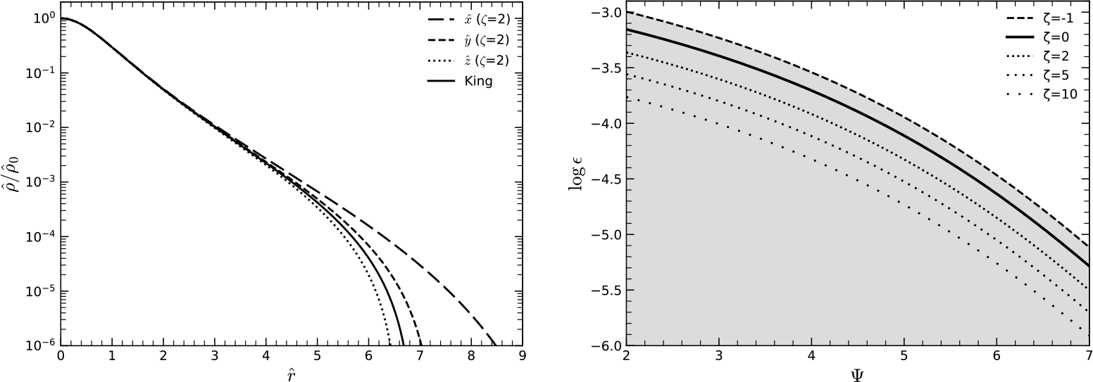
. The models have a triaxial structure, as illustrated by the density profiles in Fig. 1. Relative to a spherical King (Reference King1966) model of equal concentration, there is significant extension along the
 $\hat{x}$
-axis, compression along the
 $\hat{z}$
-axis (the axis of rotation), and either extension or compression along the
 $\hat{y}$
-axis, depending on parameter values. At constant concentration and tidal strength parameter, the overall deviation from sphericity increases in magnitude with the value of the asynchronicity parameter. The velocity dispersion, which is isotropic by definition and, like all velocity moments, a monotonic function of
 $\varPsi$
, exhibits the same pattern of elongation and compression.
Left: Density profiles, normalised to their central value, of a first-order critical model with
 $\Psi=4$
,
 $\zeta=2$
and
 $\varepsilon=1.211\times10^{-4}$
. The galactic potential is Keplerian (
 $\nu=3$
). Also shown (solid line) is the density profile for the spherical King (Reference King1966) model with
 $\Psi=4$
. Right: The (
 $\Psi,\varepsilon$
) parameter space for first-order models with
 $\nu=3$
. The curves give the maximum allowed value of the tidal strength parameter as a function of concentration, for asynchronicities
 $\zeta\in\{-1,0,2,5,10\}$
. The shaded area gives the maximum extent of the allowed parameter space, bounded by the curve for
 $\zeta=-1$
(
 $\omega=0$
).

The right panel of Fig. 1 shows the
 $(\Psi,\varepsilon)$
parameter space. The plotted curves give the maximum allowed value of
 $\varepsilon$
, over a range of
 $\Psi$
, for different values of
 $\zeta$
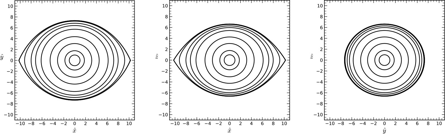
. These maximal values correspond to what we term ‘critical’ models, whose boundaries follow the outermost closed equipotential surface. Two saddle points in the total potential are found where this surface intersects with the x-axis. Critical models exhibit the maximum deviation from spherical symmetry possible for a bound system, exemplified by the sections through equipotential surfaces shown in Fig. 2. Values of
 $\varepsilon$
far below the critical value result in ‘subcritical’ models that underfill the volume bounded by the outermost closed equipotential and deviate only slightly from spherical symmetry. Increasing
 $\zeta$
is shown to lower the line of maximum
 $\varepsilon$
, thus reducing the parameter space accessible to bound models. Physically, this means weaker tidal forces are able to disrupt models with greater internal rotation.
Sections through selected equipotential surfaces for a first-order critical model with
 $\Psi=4$
,
 $\zeta=2$
and
 $\varepsilon=1.211\times10^{-4}$
. The outermost contour is the boundary surface given by
 $\varPsi(\mathbf{r},t)=0$
. The galactic potential is Keplerian (
 $\nu=3$
).

By coupling tidal and rotational perturbations, we have constructed a three-parameter family of equilibrium dynamical models to describe the internal structure and kinematics of a tidally perturbed, rotating stellar system. In considering this plausible combination of physical ingredients, these models provide a more realistic equilibrium description of Galactic globular clusters than was previously available.

 Ψ=4
 ζ=2
 ε=1.211×10⁻⁴
 ν=3
 Ψ=4
 Ψ,ε
 ν=3
 ζ∈{−1,0,2,5,10}
 ζ=−1
 ω=0
 Ψ=4
 ζ=2
 ε=1.211×10⁻⁴
 Ψ(r,t)=0
 ν=3

 Open access

