1. Introduction
We are interested in the behaviour of a dense monolayer of identical spheres that is subjected to a homogeneous simple shear. The spheres are neutrally buoyant and large enough to not experience Brownian motion. Singh & Nott (Reference Singh and Nott2000) used Stokesian dynamics (Brady & Bossis Reference Brady and Bossis1985) to simulate such a system. The spheres in their simulation were sheared by the relative motion of boundaries to which the flow spheres were attached. The spheres of the flow interacted through hydrodynamic forces and a short-range repulsive force. Singh & Nott (Reference Singh and Nott2000) measured the components of the stress and the anisotropic microstructure of near-contacting neighbours of a typical sphere. In addition to a shear stress, they measured a pressure associated with the particle phase and a difference in normal stresses.
Anisotropic microstructure, particle pressure and differences in normal stresses have been the focus of recent numerical simulations and theoretical developments. Sierou & Brady (Reference Sierou and Brady2002) employed an accelerated Stokesian dynamics simulation (Sierou & Brady Reference Sierou and Brady2001) to provide careful characterization of the microstructure and stress components, including particle pressure and differences in normal stresses, in a sheared three-dimensional non-Brownian suspension. Nazockdast & Morris (Reference Nazockdast and Morris2012a ,Reference Nazockdast and Morris b , Reference Nazockdast and Morris2013), building on earlier work by Brady & Morris (Reference Brady and Morris1997), considered a steady shearing flow of colloidal suspensions in three dimensions, set up a partial differential equation for the pair distribution function and, using an approximate solution for the velocity of equilibriated pairs of particles, obtained numerical solutions that provide information on the anisotropic distributions of particle concentration at and away from the surface of a typical sphere. The structure near the surface permits calculation of the components of the stress associated with the particle phase. Nazockdast & Morris obtained such information over ranges of volume fractions and thermal forces and tested it against the results of their numerical simulations. The predicted microstructure, particle pressure, normal stress differences and pair trajectories were in very good agreement with those measured in the simulations, except possibly at the largest volume fractions in the non-Brownian limit.
Our calculation inhabits only a corner of the parameter space explored by Nazockdast & Morris (Reference Nazockdast and Morris2012a
,Reference Nazockdast and Morris
b
, Reference Nazockdast and Morris2013); but, by being so limited, we can be more explicit and perhaps provide a more accessible framework for understanding the microstructure, particle pressure, differences in normal stresses and issues of particle rotation related to the symmetry of the stress. We focus on steady, homogeneous, shearing flows of a relatively dense monolayer of identical non-Brownian spheres in a Newtonian fluid, with viscosity
 ${\it\mu}$
, at low Reynolds numbers. The monolayer contains
 $n$
spheres of radius
 $a$
per unit area. We assume that pairs of near-contacting spheres interact through both a lubrication force and a short-range repulsive force that varies inversely with the particle separation.
We invoke force equilibrium for each sphere in a typical pair and determine the differential equations that govern the separation between the spheres as well as the orientation of the pair with respect to the flow. Integration of these differential equations and the use of a flux balance allows determination of the angular distribution of the number of near-contacting neighbours along a trajectory representative of the trajectories in a band around it that determine the stress. This distribution varies with the orientation with respect to the flow, as seen in numerical simulations (Singh & Nott Reference Singh and Nott2000; Sierou & Brady Reference Sierou and Brady2002; Nazockdast & Morris Reference Nazockdast and Morris2013). We use this distribution together with the expressions for the interparticle forces to calculate the stresses in the particle phase, and satisfy moment equilibrium by determining the difference between the average rotations of the particles and the fluid that ensures symmetry of the stress. We calculate the particle pressure and the difference in normal stresses; both are due to the presence of the repulsive force, which breaks the symmetry in the approach and departure of near-contacting neighbours (Brady & Morris Reference Brady and Morris1997). The predicted shear stress, particle pressure and difference in normal stresses are in good agreement with the results of the Stokesian dynamics simulation carried out by Singh & Nott (Reference Singh and Nott2000).
2. Model
2.1. Kinematics
Like Dratler & Schowalter (Reference Dratler and Schowalter1996) and Singh & Nott (Reference Singh and Nott2000), we consider a monolayer of identical spheres that are subject to homogeneous, steady shearing with an average rate-of-deformation tensor
 $\unicode[STIX]{x1D63F}$
and an average rate-of-rotation tensor
 $\unicode[STIX]{x1D652}$
. We focus our attention on a typical pair of nearly contacting spheres,
 $A$
and
 $B,$
and their nearly contacting neighbours, labelled
 $n$
. The spheres are assumed to interact through lubrication forces at their points of closest approach and through a short-range repulsive force of strength
 $F_{0}$
. We permit the spheres
 $A$
and
 $B$
to have translational degrees of freedom that their neighbours do not have, and we use force equilibrium to determine these translational velocities.
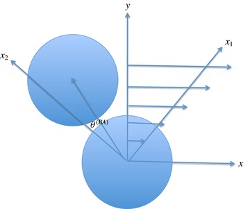
Principal directions of the flow,
 $x_{1}$
and
 $x_{2}$
, together with the angle
 ${\it\theta}^{(BA)}$
between
 $\hat{\boldsymbol{d}}^{(BA)}$
and the
 $x_{2}$
axis.

The unit vector directed from the centre of
 $A$
to the centre of
 $B$
is denoted by
 $\hat{\boldsymbol{d}}^{(BA)}$
, with
 $\hat{\boldsymbol{d}}^{(AB)}=-\hat{\boldsymbol{d}}^{(BA)}$
. We use a Cartesian coordinate system with the
 $x_{1}$
and
 $x_{2}$
axes in the directions of greatest extension and compression, respectively; see figure 1. Then, with
 ${\it\theta}^{(BA)}$
denoting the angle between
 $\hat{\boldsymbol{d}}^{(BA)}$
and the
 $x_{2}$
axis, we have
 $\hat{d}_{{\it\alpha}}^{(BA)}=(\sin {\it\theta}^{(BA)},\cos {\it\theta}^{(BA)})$
, and the components of the unit tangent vector
 $\hat{\boldsymbol{t}}^{(BA)}$
perpendicular to it are
 $t_{{\it\alpha}}^{(BA)}=\left(\cos {\it\theta}^{(BA)},-\text{sin}{\it\theta}^{(BA)}\right)$
, or
 $t_{{\it\alpha}}^{(BA)}={\it\varepsilon}_{{\it\alpha}{\it\beta}}d_{{\it\beta}}^{(BA)}$
, where
 ${\it\varepsilon}_{11}={\it\varepsilon}_{22}=0$
and
 ${\it\varepsilon}_{12}=-{\it\varepsilon}_{21}=1$
. The rotation tensor
 $\unicode[STIX]{x1D652}$
has the axial vector
 $\boldsymbol{W}^{\times }=(1/2){\it\varepsilon}_{{\it\alpha}{\it\beta}}W_{{\it\beta}{\it\alpha}}$
. The angle
 ${\it\theta}^{(BA)}$
is a function of time,
 $t$
, and we indicate derivatives with respect to
 $t$
with overdots.
We denote the velocity of the centre of sphere
 $B$
relative to that of sphere
 $A$
by
 $\boldsymbol{v}^{(BA)}$
and the average angular velocity of the spheres by
 ${\rm\Omega}^{\times }$
; the components of the tensor
 ${\it\bf\Omega}$
associated with
 ${\rm\Omega}^{\times }$
are given by
 ${\rm\Omega}_{{\it\alpha}{\it\beta}}={\it\varepsilon}_{{\it\beta}{\it\alpha}}{\rm\Omega}^{\times }$
. The distance between the centres of the neighbouring spheres
 $A$
and
 $B$
is
 $2a+s^{(BA)}$
, where
 $s^{(BA)}$
is the smallest separation between their edges. Because
 $s^{(BA)}$
is small compared to
 $a$
, we ignore it in the sum and elsewhere work to lowest order in the ratio
 $s^{(BA)}/a$
.
The velocity of the point on sphere
 $B$
closest to sphere
 $A$
relative to the velocity of the corresponding point on
 $A$
is
 $$\begin{eqnarray}v_{{\it\alpha}}^{(BA)}+2a{\rm\Omega}^{\times }\hat{t}_{a}^{(BA)},\end{eqnarray}$$
where
 $$\begin{eqnarray}v_{{\it\alpha}}^{(BA)}={\dot{s}}^{(BA)}\hat{d}_{{\it\alpha}}^{(BA)}+2a\dot{{\it\theta}}^{(BA)}\hat{t}_{{\it\alpha}}^{(BA)}.\end{eqnarray}$$
The velocity of the point of closest approach of spheres
 $A$
and
 $n$
reflects the fact that when
 $n\neq B$
, sphere
 $n$
is assumed to move with the average translation and rotation,
 $$\begin{eqnarray}2a(D_{{\it\beta}{\it\gamma}}+W_{{\it\beta}{\it\gamma}})\hat{d}_{{\it\gamma}}^{(nA)}+2a{\rm\Omega}^{\times }\hat{t}_{{\it\beta}}^{(nA)}.\end{eqnarray}$$
2.2. Forces
The force
 $\boldsymbol{F}^{(BA)}$
exerted by sphere
 $B$
on sphere
 $A$
is given by (Jeffrey & Onishi Reference Jeffrey and Onishi1984; Jeffrey Reference Jeffrey1992)
 $$\begin{eqnarray}\displaystyle F_{{\it\alpha}}^{(BA)} & = & \displaystyle 6{\rm\pi}{\it\mu}aK_{{\it\alpha}{\it\beta}}^{(BA)}v_{{\it\beta}}^{(BA)}+6{\rm\pi}{\it\mu}a^{2}\left[\frac{1}{3}\ln \left(\frac{a}{s^{(BA)}}\right)+1.27\right]W^{\times }\hat{t}_{{\it\alpha}}^{(BA)}-\frac{F_{0}}{s^{(BA)}}\hat{d}_{{\it\alpha}}^{(BA)}\nonumber\\ \displaystyle & & \displaystyle -\,9.54{\rm\pi}{\it\mu}a^{2}\left(\hat{t}_{{\it\beta}}D_{{\it\beta}{\it\xi}}\hat{d}_{{\it\xi}}\right)\hat{t}_{{\it\alpha}}^{(BA)}\nonumber\\ \displaystyle & & \displaystyle +\,a^{2}{\rm\pi}{\it\mu}\left[2\ln \left(\frac{a}{s^{(BA)}}\right)-0.96\right]\left({\rm\Omega}^{\times }-W^{\times }\right)\hat{t}_{{\it\alpha}}^{(BA)},\end{eqnarray}$$
where
 $$\begin{eqnarray}K_{{\it\alpha}{\it\beta}}^{(BA)}=\frac{1}{4}\frac{a}{s^{(BA)}}\hat{d}_{{\it\alpha}}^{(BA)}\hat{d}_{{\it\beta}}^{(BA)}+\left[\frac{1}{6}\ln \left(\frac{a}{s^{(BA)}}\right)+0.64\right]\hat{t}_{a}^{(BA)}\hat{t}_{{\it\beta}}^{(BA)};\end{eqnarray}$$
constant terms have been retained because they are of the same order as the logarithms.
When
 $n\neq B$
, the corresponding force is based on the average motion and the average separation
 $\bar{s}$
:
 $$\begin{eqnarray}\displaystyle F_{{\it\alpha}}^{(nA)} & = & \displaystyle \frac{3}{\bar{s}}a^{2}{\rm\pi}{\it\mu}\left(D_{{\it\beta}{\it\xi}}\hat{d}_{{\it\xi}}^{(nA)}\hat{d}_{{\it\beta}}^{(nA)}\right)\hat{d}_{{\it\alpha}}^{(nA)}+a^{2}{\rm\pi}{\it\mu}\left[2\ln \left(\frac{1}{\bar{s}}\right)-0.96\right]\hat{t}_{{\it\alpha}}^{(nA)}\left({\rm\Omega}^{\times }-W^{\times }\right)\nonumber\\ \displaystyle & & \displaystyle +\,a^{2}{\rm\pi}{\it\mu}\left[2\ln \left(\frac{1}{\bar{s}}\right)-1.92\right]\left(D_{{\it\beta}{\it\xi}}\hat{t}_{{\it\xi}}^{(nA)}\hat{d}_{{\it\beta}}^{(nA)}\right)\hat{t}_{{\it\alpha}}^{(nA)}-\frac{F_{0}}{\bar{s}}\hat{d}_{{\it\alpha}}^{(nA)}.\end{eqnarray}$$
2.3. Equilibrium
We write down the equations of force equilibrium for particle
 $A$
, taking into account its pairwise interaction with
 $B$
and with its neighbours at points of closest approach. In doing this, we assume that the average rotation
 ${\rm\Omega}^{\times }$
of the spheres differs from the average
 $W^{\times }$
of the mixture. The former is determined by the requirement that the stress of the aggregate be symmetric.
The force equilibrium for sphere
 $A$
is given by
 $$\begin{eqnarray}F_{{\it\alpha}}^{(BA)}+\mathop{\sum }_{n\neq B}^{N^{(A)}}F_{{\it\alpha}}^{(nA)}=0,\end{eqnarray}$$
where
 $N^{(A)}$
is the number of near-contacting neighbours of sphere
 $A$
, or
 $$\begin{eqnarray}\displaystyle 0 & = & \displaystyle 6{\rm\pi}{\it\mu}aK_{{\it\alpha}{\it\beta}}^{(BA)}v_{{\it\beta}}^{(BA)}+6{\rm\pi}{\it\mu}a^{2}\left[\frac{1}{3}\ln \left(\frac{a}{s^{(BA)}}\right)+1.27\right]W^{\times }\hat{t}_{{\it\alpha}}^{(BA)}-\frac{F_{0}}{s^{(BA)}}\hat{d}_{{\it\alpha}}^{(BA)}\nonumber\\ \displaystyle & & \displaystyle -\,9.54{\rm\pi}{\it\mu}a^{2}\left(\hat{t}_{{\it\beta}}^{(BA)}D_{{\it\beta}{\it\xi}}\hat{d}_{{\it\xi}}^{(BA)}\right)\hat{t}_{{\it\alpha}}^{(BA)}+a^{2}{\rm\pi}{\it\mu}\left[2\ln \left(\frac{a}{s^{(BA)}}\right)-0.96\right]\left({\rm\Omega}^{\times }-W^{\times }\right)\hat{t}_{{\it\alpha}}^{(BA)}\nonumber\\ \displaystyle & & \displaystyle +\,\frac{3}{\bar{s}}a^{2}{\rm\pi}{\it\mu}D_{{\it\beta}{\it\xi}}\mathop{\sum }_{n\neq B}^{N^{(A)}}\hat{d}_{{\it\xi}}^{(nA)}\hat{d}_{{\it\beta}}^{(nA)}\hat{d}_{{\it\alpha}}^{(nA)}+a^{2}{\rm\pi}{\it\mu}\left[2\ln \left(\frac{1}{\bar{s}}\right)-0.96\right]\left({\rm\Omega}^{\times }-W^{\times }\right)\mathop{\sum }_{n\neq B}^{N^{(A)}}\hat{t}_{{\it\alpha}}^{(nA)}\nonumber\\ \displaystyle & & \displaystyle +\,a^{2}{\rm\pi}{\it\mu}\left[2\ln \left(\frac{1}{\bar{s}}\right)-1.92\right]D_{{\it\beta}{\it\xi}}\mathop{\sum }_{n\neq B}^{N^{(A)}}\hat{t}_{{\it\alpha}}^{(nA)}\hat{t}_{{\it\xi}}^{(nA)}\hat{d}_{{\it\beta}}^{(nA)}-\frac{F_{0}}{\bar{s}}\mathop{\sum }_{n\neq B}^{N^{(A)}}\hat{d}_{{\it\alpha}}^{(nA)}.\end{eqnarray}$$
The force equilibrium for particle
 $B$
can be obtained from that for
 $A$
by interchanging the indices
 $A$
and
 $B$
and using the facts that the forces are equal and opposite and that
 $\hat{\boldsymbol{d}}^{(AB)}=-\hat{\boldsymbol{d}}^{(BA)}$
.
The equilibrium equations for pairs of particles are useful only if we make some assumption about the arrangement of particles that surround pairs with the same orientation.
2.4. Neighbourhood averages
We assume that the neighbourhood of sphere
 $A$
is an average neighbourhood of the aggregate. This average, indicated by an overbar, is taken over the orientations of near-contacting neighbours, other than
 $B$
, given the presence of sphere
 $B$
:
 $$\begin{eqnarray}\overline{\mathop{\sum }_{n\neq B}^{N^{(A)}}\hat{d}_{{\it\alpha}}^{(nA)}\cdots \hat{d}_{{\it\gamma}}^{(nA)}}\equiv \int _{0}^{2{\rm\pi}}I({\it\phi})\hat{d}_{{\it\alpha}}\cdots \hat{d}_{{\it\gamma}}\,\text{d}{\it\phi}\end{eqnarray}$$
where
 $I({\it\phi})\,\text{d}{\it\phi}$
is the average number of near contacts, other than
 $B$
, within the angle element
 $\text{d}{\it\phi}$
. The function
 $I({\it\phi})$
is related to the probability of finding a near-contacting neighbour at
 ${\it\phi}$
, given that there is one at
 ${\it\phi}=0$
. In the integral we use, as a first approximation, an isotropic distribution (Jenkins et al.
Reference Jenkins, La Ragione, Johnson and Makse2005)
 $$\begin{eqnarray}I({\it\phi})=\left\{\begin{array}{@{}ll@{}}0\quad & \text{if }0<{\it\phi}<{\rm\pi}/3,\\ 3(k-1)/(4{\rm\pi})\quad & \text{if }{\rm\pi}/3<{\it\phi}\,<{\rm\pi},\end{array}\right.\end{eqnarray}$$
where
 $k$
is the average number of near contacts per particle, called the coordination number. Given the presence of particle
 $B$
, this distribution function ensures that there are
 $k-1$
near contacts uniformly distributed on the remaining part of the circumference. An iterative procedure could be employed to improve upon this assumption of isotropy, using the anisotropy in the near-contacting neighbours that will be determined later.
With this distribution,
 $$\begin{eqnarray}\overline{\mathop{\sum }_{n\neq B}^{N^{(A)}}\hat{d}_{{\it\alpha}}^{(nA)}}={\it\xi}\hat{d}_{{\it\alpha}}^{(BA)},\end{eqnarray}$$
where
 ${\it\xi}=-3\sqrt{3}(k-1)/(4{\rm\pi})$
, and
 $$\begin{eqnarray}\displaystyle \overline{\mathop{\sum }_{n\neq B}^{N^{(A)}}\hat{d}_{{\it\alpha}}^{(nA)}\hat{d}_{{\it\beta}}^{(nA)}\hat{d}_{{\it\gamma}}^{(nA)}}={\it\alpha}_{1}\hat{d}_{{\it\alpha}}^{(BA)}\hat{d}_{{\it\beta}}^{(BA)}\hat{d}_{{\it\gamma}}^{(BA)}+{\it\alpha}_{2}\left({\it\delta}_{{\it\alpha}{\it\beta}}\hat{d}_{{\it\gamma}}^{(BA)}+{\it\delta}_{{\it\alpha}{\it\gamma}}\hat{d}_{{\it\beta}}^{(BA)}+{\it\delta}_{{\it\beta}{\it\gamma}}\hat{d}_{{\it\alpha}}^{(BA)}\right), & & \displaystyle\end{eqnarray}$$
where
 ${\it\alpha}_{1}=0$
and
 ${\it\alpha}_{2}=-3\sqrt{3}(k-1)/(16{\rm\pi})$
.
When phrased in terms of these averages, the forces exerted on spheres
 $A$
and
 $B$
by their neighbours are equal and opposite.
2.5. Relative motion in simple shearing
We use the neighbourhood averages in the force balance (2.8) and take its normal and tangential components to determine the evolution of
 $s^{(BA)}$
and
 ${\it\theta}^{(BA)}$
as functions of the total strain,
 ${\it\gamma}$
, in a steady homogeneous shearing flow. We focus on a typical trajectory with upstream and downstream branches and initial orientations close to a dividing streamline. We solve for the separation of a pair and their orientation along the branches as functions of the total strain.
In the homogeneous steady shearing flow,
 $D_{11}=-D_{22}=\dot{{\it\gamma}}/2$
,
 $D_{12}=D_{21}=0$
,
 $W_{12}=-W_{21}=\dot{{\it\gamma}}/2$
and
 $W_{11}=W_{22}=0$
, where the strain rate
 $\dot{{\it\gamma}}$
is a constant. In dealing with this flow, we use the dimensionless quantities
 $s\equiv s^{(BA)}/a$
and
 $F\equiv F_{0}/{\rm\pi}a^{3}{\it\mu}\dot{{\it\gamma}}$
and write
 ${\it\theta}$
for
 ${\it\theta}^{(BA)}$
. In terms of these quantities, the component of the force balance along the line containing the centres of spheres
 $A$
and
 $B$
is
 $$\begin{eqnarray}\frac{1}{s}\frac{\text{d}s}{\text{d}{\it\gamma}}=\frac{2}{3}F\left(\frac{1}{s}+\frac{{\it\xi}}{\bar{s}}\right)+\frac{2{\it\alpha}_{2}}{\bar{s}}\cos 2{\it\theta},\end{eqnarray}$$
where
 $\text{d}{\it\gamma}=\dot{{\it\gamma}}\,\text{d}t$
. The term on the left-hand side is the component of the lubrication force between spheres
 $A$
and
 $B$
. The first term on the right-hand side comprises the repulsive force exerted by sphere
 $B$
and the average of that exerted by the neighbouring spheres, and the last term is the force associated with the average motion of neighbours; it contributes to the rate of change of separation in the same way as an average pure straining motion. It is important to emphasize that the equations for separation and orientation are coupled, so that the separation is influenced by the rotation of the flow. The component of the force balance across the line of centres of the spheres is
 $$\begin{eqnarray}\displaystyle \frac{\text{d}{\it\theta}}{\text{d}{\it\gamma}} & = & \displaystyle -\frac{W^{\times }}{\dot{{\it\gamma}}}-\frac{\left[\ln (1/s)-0.48+{\it\xi}\ln (1/\bar{s})-0.48{\it\xi}\right]}{\ln (1/s)+3.81}\frac{\left({\rm\Omega}^{\times }-W^{\times }\right)}{\dot{{\it\gamma}}}\nonumber\\ \displaystyle & & \displaystyle -\,\frac{\left[3{\it\alpha}_{2}/\bar{s}-4.77+{\it\xi}\ln \left(1/\bar{s}\right)-0.96{\it\xi}\right]}{2\ln (1/s)+7.62}\sin 2{\it\theta}.\end{eqnarray}$$
Here, the product of the denominator and the sum of the rotations balances the force associated with the average pure straining motion of neighbours and additional forces with components perpendicular to the line of centres, due to the difference between the average rotation of the fluid and of the spheres that is necessary to maintain symmetry of the stress.
2.6. Circumferential distribution
We next determine the corresponding equation for the evolution of the distribution of near-contacting neighbours along the arclength
 ${\it\sigma}$
of the trajectory followed by the typical pair of spheres. This distribution is defined so that
 $\mathscr{A}({\it\sigma})\,\text{d}{\it\sigma}$
is the average number of particles in the arclength increment
 $\text{d}{\it\sigma}$
. This distribution is used to weight the contact force at an orientation along the path in the calculation of the components of the stress. Its integral around the circumference of a typical sphere is, in dimensionless terms, the product of the average number
 $k$
of near-contacting neighbours and the approximate length,
 $4{\rm\pi}$
, of the trajectory. In the part of the trajectory closest to the near-contacting sphere, the distribution
 $\mathscr{A}$
is related to the anisotropic radial distribution function
 $g(r,{\it\theta})$
through
 $\mathscr{A}=ng(2,{\it\theta}){\rm\Delta}r$
, where
 ${\rm\Delta}r$
is the width of the band.
In steady state, the flux of the distribution along the trajectory is constant, so
 $$\begin{eqnarray}\frac{\text{d}}{\text{d}{\it\sigma}}(\dot{{\it\sigma}}\mathscr{A})=0\end{eqnarray}$$
with
 $$\begin{eqnarray}\dot{{\it\sigma}}=\left[{\dot{s}}^{2}+(2+s)^{2}\dot{{\it\theta}}^{2}\right]^{1/2},\end{eqnarray}$$
where an overdot denotes a derivative with respect to time. Equation (2.15) can be integrated, but the integral condition on
 $\mathscr{A}$
is easiest to apply if we keep it as a differential equation. When the trajectory is parameterized by
 ${\it\gamma}$
, the differential equation becomes
 $$\begin{eqnarray}\frac{\text{d}\dot{{\it\sigma}}}{\text{d}{\it\gamma}}\mathscr{A}+\dot{{\it\sigma}}\frac{\text{d}\mathscr{A}}{\text{d}{\it\gamma}}=0,\end{eqnarray}$$
where
 $$\begin{eqnarray}\frac{\text{d}\dot{{\it\sigma}}}{\text{d}{\it\gamma}}=\frac{1}{\left[{\dot{s}}^{2}+(2+s)^{2}\dot{{\it\theta}}^{2}\right]^{1/2}}\left[{\dot{s}}\frac{\text{d}{\dot{s}}}{\text{d}{\it\theta}}+(2+s)\frac{\text{d}s}{\text{d}{\it\theta}}\dot{{\it\theta}}^{2}+(2+s)^{2}\dot{{\it\theta}}\frac{\text{d}\dot{{\it\theta}}}{\text{d}{\it\theta}}\right],\end{eqnarray}$$
with
 ${\dot{s}}$
and
 $\dot{{\it\theta}}$
given by (2.13) and (2.14), respectively. So
 $$\begin{eqnarray}\frac{\text{d}\mathscr{A}}{\text{d}{\it\gamma}}=-\mathscr{A}\frac{\text{d}\dot{{\it\sigma}}}{\text{d}{\it\gamma}}\frac{1}{\dot{{\it\sigma}}}.\end{eqnarray}$$
2.7. Subsidiary conditions
The condition on
 $\mathscr{A}$
that its integral along a complete trajectory be related to
 $k$
is satisfied by introducing an auxiliary function
 $$\begin{eqnarray}\mathscr{I}({\it\gamma})=\int _{\hat{{\it\gamma}}}\mathscr{A}({\it\sigma})\frac{\text{d}{\it\sigma}}{\text{d}{\it\gamma}}\,\text{d}{\it\gamma},\end{eqnarray}$$
where
 $\hat{{\it\gamma}}$
is the total strain for a particle to traverse the trajectory. The differential equation associated with this is
 $$\begin{eqnarray}\frac{\text{d}\mathscr{I}}{\text{d}{\it\gamma}}=\mathscr{A}({\it\sigma})\frac{\text{d}{\it\sigma}}{\text{d}{\it\gamma}},\end{eqnarray}$$
with boundary conditions
 $$\begin{eqnarray}\mathscr{I}(0)=0,\quad \mathscr{I}(\hat{{\it\gamma}})=k/2.\end{eqnarray}$$
Another subsidiary condition is associated with the symmetry of the stress. We shall implement it after introducing the expression for the stress.
3. Particle stress
The stress tensor is the product of the number of spheres per unit area and the integral of the force dipole of the near-contacting spheres over the distribution that governs their number density:
 $$\begin{eqnarray}\unicode[STIX]{x1D61B}_{{\it\alpha}_{{\it\beta}}}=2na\int _{{\it\sigma}}\mathscr{A}\left({\it\sigma}\right)F_{{\it\alpha}}^{(BA)}\hat{d}_{{\it\beta}}^{(BA)}\,\text{d}{\it\sigma},\end{eqnarray}$$
where
 $\boldsymbol{F}^{(BA)}$
is given by (2.4). We do not calculate the stress via the stresslet (Jeffrey Reference Jeffrey1992; Jeffrey, Morris & Brady Reference Jeffrey, Morris and Brady1993). Instead, we employ an expression introduced by Cauchy for a solid consisting of grains in contact (e.g. Love Reference Love1944, Appendix, Note B) and use the resistance matrices to construct the force between near-contacting neighbours. However, we do not assume that the average rotation of the particles is the same as that of the fluid; so the expression for the stress that we employ is not symmetric until the average rotation of the particles is taken to make it so. Nazockdast & Morris (Reference Nazockdast and Morris2012a
, Reference Nazockdast and Morris2013) obtained a similar expression for the stress by ignoring the tangential forces and using the fact that as the particle separation goes to zero, the stresslet resistances become tensor products of
 $\boldsymbol{d}/2$
and the corresponding force resistances.
The dimensionless form of the interaction force is
 $$\begin{eqnarray}\displaystyle \frac{F_{{\it\alpha}}^{(BA)}}{{\rm\pi}a^{2}{\it\mu}\dot{{\it\gamma}}} & = & \displaystyle \frac{1}{\bar{s}}\left({\it\xi}F+3{\it\alpha}_{2}\cos 2{\it\theta}\right)\hat{d}_{{\it\alpha}}^{(BA)}-\left[2\ln \left(\frac{1}{\bar{s}}\right)-0.96\right]{\it\xi}\frac{\left({\rm\Omega}^{\times }-W^{\times }\right)}{\dot{{\it\gamma}}}\,\hat{t}_{{\it\alpha}}^{(BA)}\nonumber\\ \displaystyle & & \displaystyle -\,\left[\frac{3}{\bar{s}}{\it\alpha}_{2}+{\it\xi}\ln \left(\frac{1}{\bar{s}}\right)-0.96{\it\xi}\right]\sin 2{\it\theta}\hat{t}_{{\it\alpha}}^{(BA)}.\end{eqnarray}$$
The dimensionless stress tensor,
 $t_{{\it\alpha}{\it\beta}}=\unicode[STIX]{x1D61B}_{{\it\alpha}{\it\beta}}/a{\it\mu}\dot{{\it\gamma}}$
, is
 $$\begin{eqnarray}\displaystyle t_{{\it\alpha}{\it\beta}} & = & \displaystyle 2{\it\nu}\int _{\hat{{\it\gamma}}}\mathscr{A}\left({\it\sigma}\right)\left(F\frac{{\it\xi}}{\bar{s}}+\frac{3{\it\alpha}_{2}}{\bar{s}}\cos 2{\it\theta}\right)\hat{d}_{{\it\alpha}}\hat{d}_{{\it\beta}}\frac{\text{d}{\it\sigma}}{\text{d}{\it\gamma}}\,\text{d}{\it\gamma}\nonumber\\ \displaystyle & & \displaystyle -\,2{\it\nu}\int _{\hat{{\it\gamma}}}\mathscr{A}\left({\it\sigma}\right)\left[\frac{3}{\bar{s}}{\it\alpha}_{2}+{\it\xi}\ln \left(\frac{1}{\bar{s}}\right)-0.96{\it\xi}\right]\sin 2{\it\theta}\hat{t}_{{\it\alpha}}\hat{d}_{{\it\beta}}\frac{\text{d}{\it\sigma}}{\text{d}{\it\gamma}}\,\text{d}{\it\gamma}\nonumber\\ \displaystyle & & \displaystyle -\,2{\it\nu}\int _{\hat{{\it\gamma}}}\mathscr{A}\left({\it\sigma}\right)\left[2\ln \left(\frac{1}{\bar{s}}\right)-0.96\right]{\it\xi}\frac{\left({\rm\Omega}^{\times }-W^{\times }\right)}{\dot{{\it\gamma}}}\hat{t}_{{\it\alpha}}\hat{d}_{{\it\beta}}\frac{\text{d}{\it\sigma}}{\text{d}{\it\gamma}}\,\text{d}{\it\gamma}.\end{eqnarray}$$
The requirement that the stress be symmetric,
 ${\it\varepsilon}_{{\it\alpha}{\it\beta}}t_{{\it\alpha}{\it\beta}}=0$
, determines the difference between the average rotation of the spheres and the average rotation of the mixture:
 $$\begin{eqnarray}\frac{{\rm\Omega}^{\times }-W^{\times }}{\dot{{\it\gamma}}}=-\frac{\left[3{\it\alpha}_{2}/\bar{s}+{\it\xi}\ln \left(1/\bar{s}\right)-0.96{\it\xi}\right]}{k{\it\xi}\left[\ln \left(1/\bar{s}\right)-0.48\right]}\int _{\hat{{\it\gamma}}}A\left({\it\sigma}\right)\sin 2{\it\theta}\frac{\text{d}{\it\sigma}}{\text{d}{\it\gamma}}\,\text{d}{\it\gamma}.\end{eqnarray}$$
To implement this in the numerical calculation, we introduce another subsidiary function
 $$\begin{eqnarray}\mathscr{J}({\it\gamma})=\int _{\hat{{\it\gamma}}}\mathscr{A}({\it\sigma})\sin 2{\it\theta}\frac{\text{d}{\it\sigma}}{\text{d}{\it\gamma}}\,\text{d}{\it\gamma}.\end{eqnarray}$$
Then
 $$\begin{eqnarray}\frac{\text{d}\mathscr{J}({\it\gamma})}{\text{d}{\it\gamma}}=\mathscr{A}({\it\sigma})\sin 2{\it\theta}\frac{\text{d}{\it\sigma}}{\text{d}{\it\gamma}},\end{eqnarray}$$
with boundary conditions
 $$\begin{eqnarray}\mathscr{J}(0)=0,\quad \mathscr{J}(\hat{{\it\gamma}})=\frac{{\rm\Omega}^{\times }-W^{\times }}{\dot{{\it\gamma}}}\frac{k{\it\xi}\left[0.48-\ln (1/\bar{s})\right]}{\left[3{\it\alpha}_{2}/\bar{s}+{\it\xi}\ln (1/\bar{s})-0.96{\it\xi}\right]}.\end{eqnarray}$$
With the determination of the difference in average rotations, we obtain the final expression of the stress through (3.3). From this, we determine the particle pressure, the difference in normal stresses and the shear stress. The particle pressure is
 $$\begin{eqnarray}p=-\frac{1}{2}(t_{11}+t_{22})=-\frac{{\it\nu}}{\bar{s}}\int _{\hat{{\it\gamma}}}\mathscr{A}({\it\sigma})\left({\it\xi}F+3{\it\alpha}_{2}\cos 2{\it\theta}\right)\frac{\text{d}{\it\sigma}}{\text{d}{\it\gamma}}\,\text{d}{\it\gamma}\end{eqnarray}$$
and, in the principal axes coordinate system, the difference
 $N$
between the components of the stress parallel and perpendicular to the flow is
 $$\begin{eqnarray}N=-2t_{12},\end{eqnarray}$$
or
 $$\begin{eqnarray}\displaystyle N & = & \displaystyle -2\frac{{\it\nu}}{\bar{s}}\int _{\hat{{\it\gamma}}}\mathscr{A}({\it\sigma})\left({\it\xi}F+3{\it\alpha}_{2}\cos 2{\it\theta}\right)\sin 2{\it\theta}\frac{\text{d}{\it\sigma}}{\text{d}{\it\gamma}}\,\text{d}{\it\gamma}\nonumber\\ \displaystyle & & \displaystyle +\,4{\it\nu}\int _{\hat{{\it\gamma}}}\mathscr{A}({\it\sigma})\left[\frac{3}{\bar{s}}{\it\alpha}_{2}+{\it\xi}\ln \left(\frac{1}{\bar{s}}\right)-0.96{\it\xi}\right]\sin 2{\it\theta}\cos ^{2}{\it\theta}\frac{\text{d}{\it\sigma}}{\text{d}{\it\gamma}}\,\text{d}{\it\gamma}\nonumber\\ \displaystyle & & \displaystyle +\,4{\it\nu}\int _{\hat{{\it\gamma}}}\mathscr{A}({\it\sigma})\left[2\ln \left(\frac{1}{\bar{s}}\right)-0.96\right]{\it\xi}\frac{\left({\rm\Omega}^{\times }-W^{\times }\right)}{\dot{{\it\gamma}}}\cos ^{2}{\it\theta}\frac{\text{d}{\it\sigma}}{\text{d}{\it\gamma}}\,\text{d}{\it\gamma}.\end{eqnarray}$$
The shear stress
 ${\it\tau}_{xy}$
is, in dimensionless terms,
 $$\begin{eqnarray}{\it\tau}_{xy}=\frac{t_{11}-t_{22}}{2},\end{eqnarray}$$
or
 $$\begin{eqnarray}\displaystyle {\it\tau}_{xy} & = & \displaystyle -\frac{{\it\nu}}{\bar{s}}\int _{\hat{{\it\gamma}}}\mathscr{A}({\it\sigma})[{\it\xi}F+3{\it\alpha}_{2}\cos 2{\it\theta}]\cos 2{\it\theta}\frac{\text{d}{\it\sigma}}{\text{d}{\it\gamma}}\,\text{d}{\it\gamma}\nonumber\\ \displaystyle & & \displaystyle -\,{\it\nu}\left[\frac{3}{\bar{s}}{\it\alpha}_{2}+{\it\xi}\ln \left(\frac{1}{\bar{s}}\right)-0.96{\it\xi}\right]\int _{\hat{{\it\gamma}}}\mathscr{A}({\it\sigma})\sin ^{2}2{\it\theta}\frac{\text{d}{\it\sigma}}{\text{d}{\it\gamma}}\,\text{d}{\it\gamma}\nonumber\\ \displaystyle & & \displaystyle -\,{\it\nu}\left[2\ln \left(\frac{1}{\bar{s}}\right)-0.96\right]{\it\xi}\frac{\left({\rm\Omega}^{\times }-W^{\times }\right)}{\dot{{\it\gamma}}}\int _{\hat{{\it\gamma}}}\mathscr{A}({\it\sigma})\sin 2{\it\theta}\frac{\text{d}{\it\sigma}}{\text{d}{\it\gamma}}\,\text{d}{\it\gamma},\end{eqnarray}$$
where
 $x$
is the direction of the flow and
 $y$
is the direction perpendicular to it.
We note that the normal and tangential components of the lubrication force both contribute to the difference in normal stresses
 $N$
.
4. Numerical results
In order to make quantitative predictions about the components of the particle stress, we must specify the average separation,
 $\bar{s}$
, and the average number
 $k$
of near-contacting neighbours of a given particle, i.e. the coordination number. Both quantities are expected to be functions of the area fraction, with
 $\bar{s}$
having a stronger dependence than
 $k$
in dense flows. An analytical relation between the area fraction
 ${\it\nu}=n{\rm\pi}a^{2}$
and the average separation
 $\bar{s}$
between nearest neighbours in an isotropic, thermally equilibrated aggregate of colliding circular disks is given by (Torquato Reference Torquato1995)
 $$\begin{eqnarray}\bar{s}=\frac{{\rm\pi}^{1/2}}{8G},\end{eqnarray}$$
where
 $$\begin{eqnarray}G\equiv \frac{{\it\nu}(1-7{\it\nu}/16)}{(1-{\it\nu})^{2}}.\end{eqnarray}$$
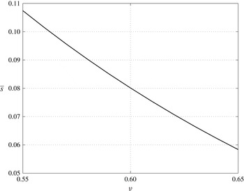
In figure 2, we show the behaviour of this average separation
 $\bar{s}$
as a function of the area fraction
 ${\it\nu}$
.
Plot of average separation
 $\overline{s}$
versus area fraction
 ${\it\nu}$
.

In the absence of an expression suitable for the trajectories of near-contacting neighbours in the anisotropic environment of simple shearing, we use this expression to relate the average separation in a typical trajectory to the area fraction. This relation might also serve as the first step in an iterative scheme that would include the predicted anisotropy. We take
 $k=3$
because, with the above relation between
 $\bar{s}$
and
 ${\it\nu}$
, it provides a good fit to the values of the shear stress measured by Singh & Nott (Reference Singh and Nott2000).
We use the Matlab function bvp4c to solve the two-point boundary value problem described in § 2. The Matlab m-files for the ordinary differential equations and boundary conditions are given in the Appendix. The trajectory that we focus on is representative of those in its neighbourhood, which determine the microstructure and the stress. The trajectory has an upstream branch and a downstream branch. The branches are initiated at positions on either side of a dividing streamline at a separation of
 $s=0.1$
. We consider the first single-valued trajectory upstream of the dividing streamline to be the upstream branch of the representative trajectory. The downstream branch is then taken to be the part of the trajectory completed in the same amount of strain
 ${\it\gamma}$
. Then, the spheres upstream of the dividing streamline approach close to the compression axis and depart from close to the extension axis. The spheres downstream of the dividing streamline approach and depart from nearer the
 $x$
-axis. The distributions of particles are defined along these branches and are related to the average number of near-contacting neighbours per particle in proportion to their length.
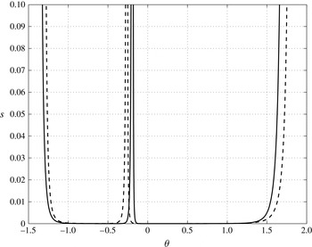
In figure 3 we plot the edge separation,
 $s$
, as a function of
 ${\it\theta}$
, for
 $k=3$
and a dimensionless repulsive strength of
 $10^{-4}$
, for values of the area fraction
 ${\it\nu}=0.55$
and
 $0.65$
. Again,
 ${\it\theta}=0$
is in the direction of the principal compression. When
 $F$
equals zero, there is contact between the surfaces of the two spheres for
 $-{\rm\pi}/4\leqslant {\it\theta}\leqslant {\rm\pi}/4$
; when
 $F$
is different from zero, there is a minimum separation between the surfaces of the spheres.
Plots of the separation
 $s$
versus
 ${\it\theta}$
, with
 $k=3$
and
 $F=10^{-4}$
, for
 ${\it\nu}=0.55$
(dashed) and
 ${\it\nu}=0.65$
(solid).

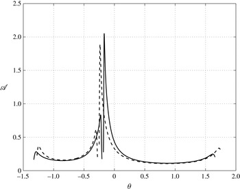
In figure 4 we plot the particle distributions
 $\mathscr{A}$
against
 ${\it\theta}$
, again for
 $k=3$
, a dimensionless repulsive strength of
 $10^{-4}$
and values of the area fraction
 ${\it\nu}=0.55$
and
 $0.65$
. The shapes of these distributions are similar to those measured by Singh & Nott (Reference Singh and Nott2000) in their simulation of a monolayer and by Sierou & Brady (Reference Sierou and Brady2002), Nazockdast & Morris (Reference Nazockdast and Morris2013) on the central plane of their three-dimensional simulations. The distribution takes its largest values near the direction of greatest compression. The distributions are not symmetric about
 ${\it\theta}=0$
, because of the rotation,
 $W^{\times }$
, of the flow. In pure straining,
 $W^{\times }=0$
and there is symmetry. When
 $F$
is different from zero, the distribution is not symmetric about
 $+{\rm\pi}/4$
and
 $-{\rm\pi}/4$
; this asymmetry is associated with the existence of the particle pressure and the difference in normal stresses. The vertical lines in the distribution correspond to the parts of the trajectory approaching the surface from the initial separation of 0.1. The contribution of these parts to the stress is negligible, but they do contribute to
 $k$
.
Plots of the particle distribution
 $\mathscr{A}$
versus
 ${\it\theta}$
, with
 $k=3$
and
 $F=10^{-4}$
, for
 ${\it\nu}=0.55$
(dashed) and
 ${\it\nu}=0.65$
(solid).

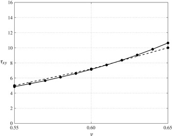
In figure 5 we plot the shear stress
 ${\it\tau}_{xy}$
versus
 ${\it\nu}$
and compare the values with those measured by Singh & Nott (Reference Singh and Nott2000). The predicted shear stress is close to what Singh & Nott (Reference Singh and Nott2000) measured, and the qualitative behaviour is similar to what they observed. In order for the stress to be symmetric,
 ${\rm\Omega}^{\times }-W^{\times }$
must equal 0.49, larger than expected and more than twice that measured by Drazer et al. (Reference Drazer, Koplik, Khusid and Acrivos2004) in numerical simulations of three-dimensional shearing flows of spheres at lower equivalent solid fractions. More measurements of the average rotation of the particles in dense non-Brownian shearing flows are needed.
Predicted shear stress
 ${\it\tau}_{xy}$
plotted against the area fraction
 ${\it\nu}$
(solid line connecting predicted values), for coordination number
 $k=3$
and repulsive force
 $F=10^{-4}$
, compared with the values measured by Singh & Nott (Reference Singh and Nott2000) (dashed line connecting measured values).

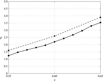
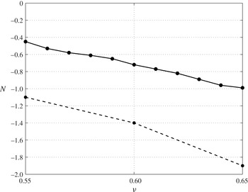
In the modelling and calculations here, our primary interest is not in the shear stress but in the particle pressure and the normal stress difference. These are effects that depend on the presence of the repulsive force. We plot the particle pressure and the difference in normal stresses versus
 ${\it\nu}$
in figures 6 and 7, respectively.
Predicted particle pressure
 $p$
plotted against the area fraction
 ${\it\nu}$
(solid line connecting predicted values), for coordination number
 $k=3$
and repulsive force
 $F=10^{-4}$
, compared with the values measured by Singh & Nott (Reference Singh and Nott2000) (dashed line connecting measured values).

Predicted normal stress difference
 $N$
plotted against the area fraction
 ${\it\nu}$
(solid line connecting predicted values), for coordination number
 $k=3$
and repulsive force
 $F=10^{-4}$
, compared with the values measured by Singh & Nott (Reference Singh and Nott2000) (dashed line connecting measured values).

The predicted particle pressure and difference in normal stresses have the same order of magnitude and the same behaviour with respect to the area fraction as the values measured by Singh & Nott (Reference Singh and Nott2000). They owe their existence to the asymmetry of the distribution function about
 ${\it\theta}=\pm {\rm\pi}/4$
, which is associated with the presence of the repulsive force in the numerical simulations and the present calculations (Brady & Morris Reference Brady and Morris1997). As might be expected, the components of the stress are sensitive to
 $k$
. A 10 % decrease in coordination number leads to approximately 25 % decreases in
 ${\it\tau}_{xy}$
,
 $p$
and
 $N$
.
We find that
 ${\it\tau}_{xy}$
is essentially independent of
 $F$
, while
 $p$
increases and
 $N$
decreases as
 $F$
increases. The explicit forms of the expressions for
 $\text{d}s/\text{d}{\it\gamma}$
and
 $\text{d}{\it\theta}/\text{d}{\it\gamma}$
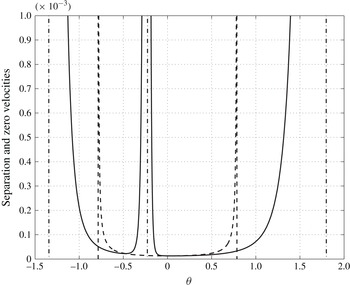
permit us to say something about their dependence. In figure 8 we show an expanded view of
 $s$
versus
 ${\it\theta}$
on which curves of
 $\text{d}s/\text{d}{\it\gamma}=0$
and
 $\text{d}{\it\theta}/\text{d}{\it\gamma}=0$
have been superimposed.
Expanded view of
 $s$
versus
 ${\it\theta}$
(solid), for
 ${\it\nu}=0.60$
,
 $k=3$
and
 $F=10^{-4}$
, together with curves of
 ${\dot{s}}=0$
(dashed) and
 $\dot{{\it\theta}}=0$
(dot-dashed).

On the curve
 $\text{d}s/\text{d}{\it\gamma}=0$
,
 $$\begin{eqnarray}s=-\frac{\overline{s}}{{\it\xi}+(2{\it\alpha}_{2}/F)\cos 2{\it\theta}}\doteq -\frac{\overline{s}F}{2{\it\alpha}_{2}\cos 2{\it\theta}}.\end{eqnarray}$$
That is, the minimum value of
 $s$
is proportional to
 $F$
. Upon introducing the positive constants
 $a=0.48(1+{\it\xi})-{\it\xi}\ln (1/\overline{s})$
and
 $b=[-3{\it\alpha}_{2}/\overline{s}-{\it\xi}\ln (1/\overline{s})+0.96{\it\xi}+4.77]/2$
, we may estimate
 $\mathscr{A}$
as follows:
 $$\begin{eqnarray}\displaystyle \mathscr{A} & \propto & \displaystyle \frac{1}{\dot{{\it\theta}}}=\frac{\ln (1/s)+3.81}{-W^{\times }(a+3.81)-\left[\ln (1/s)-a\right]{\rm\Omega}^{\times }+b\sin 2{\it\theta}}\nonumber\\ \displaystyle & \doteq & \displaystyle \frac{\ln (1/s)+3.81}{-W^{\times }(a+3.81)+b\sin 2{\it\theta}}.\end{eqnarray}$$
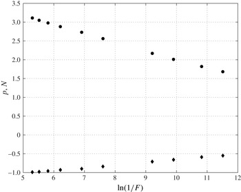
That is, along this curve,
 $\mathscr{A}$
is proportional to
 $\ln (1/F)$
. Because the trajectory follows the curve for a significant interval, this suggests that
 $p$
and
 $N$
also vary with
 $\ln (1/F)$
. In figure 9, we test this hypothesis.
Plots of particle pressure
 $p$
(circles) and normal stress difference
 $N$
(diamonds) versus
 $\ln (1/F)$
, for coordination number
 $k=3$
and
 ${\it\nu}=0.6$
.

The plot in figure 9 indicates that
 $p$
and
 $N$
vary linearly with
 $\ln (1/F)$
. We should mention that the repulsive force that we employ has a simpler form than that used by Singh & Nott (Reference Singh and Nott2000) and others (e.g. Sierou & Brady Reference Sierou and Brady2002). Their force involves both a magnitude and a range. However, for the particle separations on which the calculation of the stress is based, the simpler form that we use is indistinguishable from theirs for all but dimensionless ranges smaller than
 $10^{-4}$
.
5. Conclusion
We have introduced degrees of freedom associated with the relative translation and rotation of pairs of near-contacting particles in a dense, slow, shearing flow of a monolayer of spheres suspended in a viscous liquid. A short-range repulsive force is assumed to break the symmetry of the approach and departure of a pair. The introduction of force equilibrium and an assumption regarding the typical neighbourhood of a pair permit the determination of the components of relative velocity along and across the line of centres.
Integration of the equations for the velocities along a typical particle trajectory and the introduction of a flux balance permits the determination of the distribution of spheres about the circumference of a typical sphere. Stresses based on this distribution include a particle pressure and a difference in normal stresses parallel to and across the flow. To ensure the symmetry of the stress, given the anisotropy in particle distribution, the average rotation of the spheres must differ from the average rotation of the flow. The predictions of the dependence of the particle distribution on orientation and the variation of stresses on the area fraction are in relatively good agreement with the results of numerical simulations.
Earlier, the more phenomenological studies of Phan-Thien (Reference Phan-Thien1995), Goddard (Reference Goddard2006) and Stickel, Phillips & Powell (Reference Stickel, Phillips and Powell2006) focused on the evolution of low moments of the particle distribution, with Phan-Thien (Reference Phan-Thien1995) and Goddard (Reference Goddard2006) considering purely hydrodynamic interactions. The determination of the complete distribution in the context of so simple and explicit a theory as we have outlined here can inform decisions made in developing such theories for the low moments.
Acknowledgements
This research was supported in part by the National Science Foundation under grant no. NSF PHY11-25915 to the Kavli Institute of Theoretical Physics, by the Office of Naval Research Global under grant N62909-13-1-V152 and by G.N.F.M. (Italy). J.T.J. is grateful to the Politecnico di Bari for support of research visits.
Appendix
Here we provide the Matlab m-files for the ordinary differential equations and boundary conditions solved in the numerical calculations of § 4.