1 Introduction
Ringing is of concern in survival conditions for gravity-based structures (GBSs) and tension leg platforms (TLPs) in deep water. Ringing is caused by extreme waves exciting transient resonant response of global structural modes. The relevant resonance periods are significantly lower than the typical peak periods,
 $T_{p}$
, of the wave spectrum in larger sea states. The interesting natural periods for a TLP and a GBS are approximately one-fourth and one-third of
 $T_{p}$
respectively. This means that third and fourth harmonic load terms are needed in the analysis. Ringing of an offshore wind turbine monopile in intermediate depth wave conditions has recently gained interest.
Experimental studies of ringing, including irregular and regular waves, are described, for instance, by Grue, Bjorshol & Strand (Reference Grue, Bjorshol and Strand1994), Chaplin, Rainey & Yemm (Reference Chaplin, Rainey and Yemm1997) and Huseby & Grue (Reference Huseby and Grue2000). A recent numerical study was presented in Paulsen et al. (Reference Paulsen, Bredmose, Bingham and Jacobsen2014). There are, in particular, two phenomena that are discussed vigorously. One is the so-called secondary load cycle that occurs in steep wave cases – a distinct peak in the load time series following the main load peak. The other is a local rear run-up, which is discussed in relation to the first phenomenon. Discrepancies between theoretically and experimentally obtained third harmonics of the force for long and steep waves have also been noted. In the present study, this is discussed in detail. We associate the discrepancies with the local rear run-up.
Analytic studies on ringing loads on a fixed and non-moving vertical surface-piercing circular cylinder standing on the sea floor in deep water incident waves were reported by Faltinsen, Newman & Vinje (Reference Faltinsen, Newman and Vinje1995) (FNV) and by Newman (Reference Newman, Grue, Gjevik and Weber1996). Faltinsen et al. (Reference Faltinsen, Newman and Vinje1995) assumed regular incident waves and Newman considered irregular waves. Faltinsen (Reference Faltinsen1999) generalized the FNV method to a monotower with non-circular cross-sections varying along the cylinder axis. The cross-section had two symmetry planes. The waves were long crested and propagated along one of the symmetry axes. No far-field wave generation was predicted by the model. Malenica & Molin (Reference Malenica and Molin1995) developed a complete third-order diffraction model, including far-field wave generation, in finite water depth.
The present paper generalizes the FNV method to finite water depth. By generalization, we mean that the incident wave kinematics for finite water depth is used rather than that for deep water. Further, arbitrary (high-order) wave theory or numerically calculated wave kinematics may be used in the generalized formula; it is shown how the generalized FNV theory can be used more generally in combination with a numerical wave tank generating non-breaking waves, including irregular waves. In the present study, we combine the FNV method in finite water depth with third- and fifth-order Stokes wave theory. The limitation of Stokes theory is discussed in terms of the Ursell number.
The main focus in this paper is on horizontal wave loads (forces and moments) oscillating with frequency
 $3\unicode[STIX]{x1D714}$
in regular incident waves. However, load terms oscillating with frequencies of
 $\unicode[STIX]{x1D714}$
,
 $2\unicode[STIX]{x1D714}$
,
 $4\unicode[STIX]{x1D714}$
and
 $5\unicode[STIX]{x1D714}$
are also studied. It is demonstrated that the second- and third-order incident wave potentials, which are zero in deep water, give major contributions in finite water depths. The theory is validated by comparing with novel model tests covering regular wave conditions. For the third harmonic of the loads, the agreement is good for small to medium wave steepnesses, while, above a certain limit, there is, in general, a monotonically increasing discrepancy with increasing wave steepness.
The FNV method for the horizontal loads contains a mass term similar to that in Morison’s equation with inertia coefficient equal to two. However, there are additional important terms in the FNV method that are not included in Morison’s equation. One difference comes from a force term arising because approximate nonlinear free-surface conditions are satisfied in the FNV method. This term is important for the loads oscillating with frequency
 $3\unicode[STIX]{x1D714}$
in deep water, where
 $\unicode[STIX]{x1D714}$
is the wave frequency. The importance of the term diminishes with decreasing water depth.
The paper is organized as follows. The generalized FNV theory is presented in § 2. The experimental set-up is described in § 3. The experimental accuracy and measurement errors are discussed in some detail. The results are presented in § 4. The computed horizontal force and mudline moments are compared with the experimental data. Summarizing comments are given in § 5.
2 Theory
The original FNV theory by Faltinsen et al. (Reference Faltinsen, Newman and Vinje1995) considered infinite water depth and regular incident third-order Stokes waves with frequency
 $\unicode[STIX]{x1D714}$
. Horizontal loads oscillating with frequencies
 $\unicode[STIX]{x1D714}$
,
 $2\unicode[STIX]{x1D714}$
and
 $3\unicode[STIX]{x1D714}$
were derived. The incident waves are characterized by a wave amplitude
 $\unicode[STIX]{x1D701}_{a}$
of the same order of magnitude as a characteristic cross-dimensional length of the structure. The theory assumes that the wavelengths,
 $\unicode[STIX]{x1D706}$
, are long compared with the cylinder radius
 $a$
, i.e. that the non-dimensional wavenumber
 $ka=2\unicode[STIX]{x03C0}a/\unicode[STIX]{x1D706}$
is sufficiently small so that far-field wave generation by the structure can be neglected. The incident wave slope is sufficiently small to avoid wave breaking. Viscous flow separation is neglected, which means that the Keulegan–Carpenter (
 $KC$
) number is sufficiently small.
We generalize the FNV theory to account for arbitrary (high-) order incident wave kinematics, and to finite water depth
 $h$
.
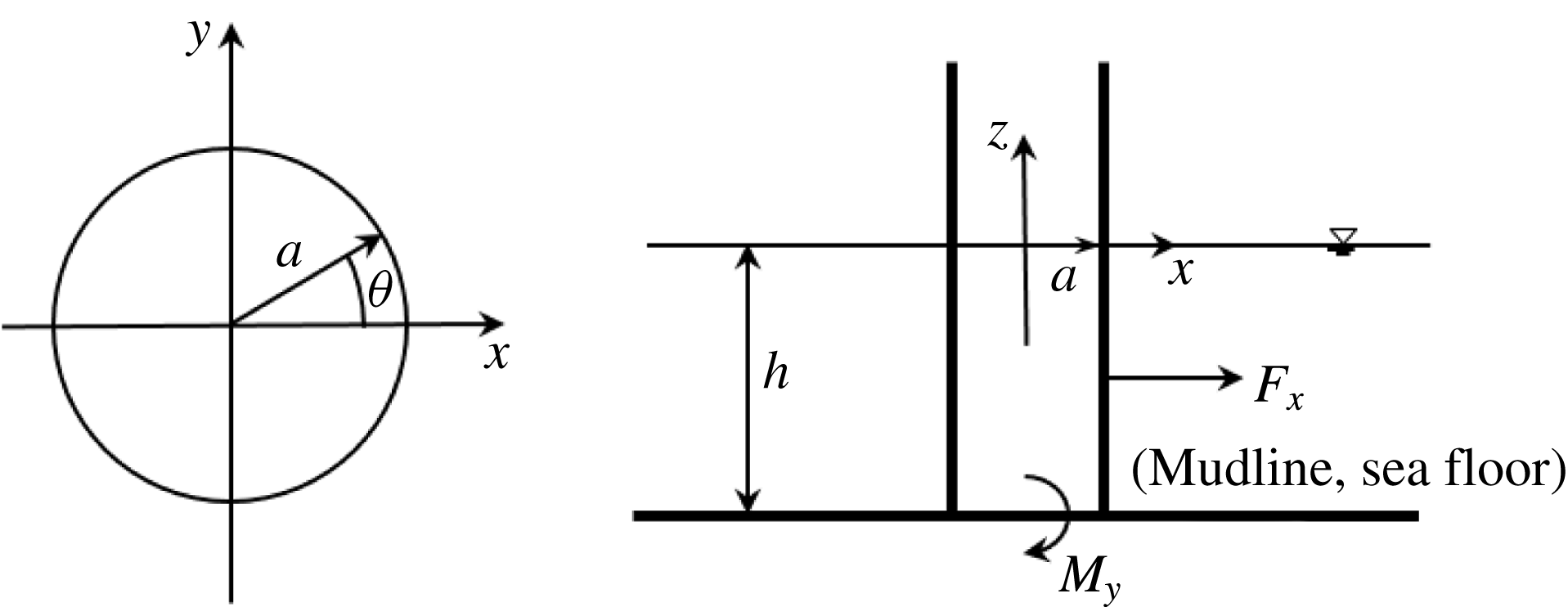
Description of the coordinate system
 $Oxyz$
, the load conventions, the water depth
 $h$
, the cylinder radius
 $a$
and the angle
 $\unicode[STIX]{x1D703}$
.
 $F_{x}$
and
 $M_{y}$
denote the horizontal force and mudline overturning moments, respectively. The incident waves propagate along the positive
 $x$
-direction.

2.1 FNV formulation in finite water depth
We consider gravity waves with wavelength
 $\unicode[STIX]{x1D706}$
, incident on a vertical surface-piercing and non-moving circular cylinder with cross-sectional radius
 $a$
standing on the sea floor in finite water depth
 $h$
; see figure 1. We define a Cartesian coordinate system
 $Oxyz$
with the
 $z$
-axis along the cylinder axis and with positive direction upwards. Furthermore,
 $z=0$
and
 $z=-h$
correspond to the calm free surface and the sea floor respectively. The positive
 $x$
-direction is along the incident wave-propagation direction. The water has infinite horizontal extent.
In the original FNV theory, a small parameter
 $\unicode[STIX]{x1D716}$
was introduced and both the linear incident wave slope
 $k\unicode[STIX]{x1D701}_{a}$
and the non-dimensional cylinder radius
 $ka$
were of
 $O(\unicode[STIX]{x1D716})$
. The total potential was expressed as
 $\unicode[STIX]{x1D711}=\unicode[STIX]{x1D711}_{I}+\unicode[STIX]{x1D711}_{s}+\unicode[STIX]{x1D713}$
, where
 $\unicode[STIX]{x1D711}_{D}=\unicode[STIX]{x1D711}_{I}+\unicode[STIX]{x1D711}_{s}$
is a diffraction potential satisfying the two-dimensional Laplace equation in each horizontal plane up to and including the incident free surface and
 $\unicode[STIX]{x1D713}$
is a third-order potential satisfying the three-dimensional Laplace equation and approximate free-surface conditions to third order. Here,
 $\unicode[STIX]{x1D711}_{I}$
represents the incident wave potential. These features are all retained in finite water depth.
In § 2.2, the main expressions of the load model are given. A brief outline of the derivation is next provided in § 2.3. All expressions are valid for both deep water and finite water depths. It should be noted, however, that the third-order incident potential is zero in deep water, whereas it is a dominant contributor to the third harmonic load in finite water depth.
2.2 Generalized FNV load model
The total load is obtained by integrating the distributed horizontal hydrodynamic force
 $F^{\prime }$
due to
 $\unicode[STIX]{x1D711}_{D}$
along the cylinder up to the incident free surface, and adding the load term due to
 $\unicode[STIX]{x1D713}$
,
 $$\begin{eqnarray}F_{x}=\int _{-h}^{\unicode[STIX]{x1D701}_{I}}F^{\prime }(z,t)\,\text{d}z+F^{\unicode[STIX]{x1D713}}.\end{eqnarray}$$
The distributed load term
 $F^{\prime }$
due to
 $\unicode[STIX]{x1D711}_{D}$
is
 $$\begin{eqnarray}\displaystyle F^{\prime }(z,t)=\unicode[STIX]{x1D70C}\unicode[STIX]{x03C0}a^{2}\left(\frac{\unicode[STIX]{x2202}u}{\unicode[STIX]{x2202}t}+u\frac{\unicode[STIX]{x2202}u}{\unicode[STIX]{x2202}x}+w\frac{\unicode[STIX]{x2202}u}{\unicode[STIX]{x2202}z}\right)+a_{11}\left(\frac{\unicode[STIX]{x2202}u}{\unicode[STIX]{x2202}t}+w\frac{\unicode[STIX]{x2202}u}{\unicode[STIX]{x2202}z}\right)\quad \text{for }h\leqslant z\leqslant \unicode[STIX]{x1D701}_{I}, & & \displaystyle\end{eqnarray}$$
where
 $\unicode[STIX]{x1D70C}$
is the mass density of water,
 $a_{11}=\unicode[STIX]{x1D70C}\unicode[STIX]{x03C0}a^{2}$
is the 2D added mass in surge,
 $\unicode[STIX]{x1D701}_{I}$
is the incident wave elevation (to any order) at
 $x=0$
,
 $\unicode[STIX]{x1D711}_{I}$
is the incident wave potential (to corresponding order),
 $u=\unicode[STIX]{x2202}\unicode[STIX]{x1D711}_{I}/\unicode[STIX]{x2202}x|_{x=0},\,\unicode[STIX]{x2202}u/\unicode[STIX]{x2202}x=\unicode[STIX]{x2202}^{2}\unicode[STIX]{x1D711}_{I}/\unicode[STIX]{x2202}x^{2}|_{x=0}$
and
 $w=\unicode[STIX]{x2202}\unicode[STIX]{x1D711}_{I}/\unicode[STIX]{x2202}z|_{x=0}$
. The horizontal force due to
 $\unicode[STIX]{x1D713}$
is, no differently from in the deep water case,
 $$\begin{eqnarray}\displaystyle F^{\unicode[STIX]{x1D713}}=\unicode[STIX]{x1D70C}\unicode[STIX]{x03C0}a^{2}\frac{4}{g}u^{2}\frac{\unicode[STIX]{x2202}u}{\unicode[STIX]{x2202}t}, & & \displaystyle\end{eqnarray}$$
where the quantities are evaluated at
 $x=0$
,
 $z=0$
. The centre of action of
 $F^{\unicode[STIX]{x1D713}}$
is at
 $z=0$
.
The generalized formulation (2.1)–(2.2) is consistent with the original FNV method to third order, as long as the incident wave potential,
 $\unicode[STIX]{x1D711}_{I}$
, to at least third order is used. If higher-order wave kinematics is used, higher-order load terms appear in the incident wave only. The generalized formulation allows for any regular wave theory, a numerical wave tank and irregular long-crested incident waves to be applied, as long as the local wave slope is not so large that the waves are breaking. The influence of the sea floor topography with small changes in the
 $x$
-direction can be considered, as long as there are no sea bottom changes in the
 $y$
-direction. The numerical wave tank must be based on potential-flow theory of incompressible water and can account for exact nonlinear free-surface conditions. Breaking waves can implicitly not be analysed. Essential assumptions in the load formula are also that wave generation by the cylinder and flow separation are secondary and can be neglected. The latter is not generally true, however, as is discussed throughout the paper. The moment is calculated by multiplying with the wanted arm inside the integration of (2.2) and the term (2.3). Computational time makes it realistic to simulate many realizations of different sea states.
The most common version of Morison’s equation within potential-flow theory expresses
 $F^{\prime }$
as
 $(\unicode[STIX]{x1D70C}\unicode[STIX]{x03C0}a^{2}+a_{11})\unicode[STIX]{x2202}u/\unicode[STIX]{x2202}t$
. Another version is to use the total advection term
 $\unicode[STIX]{x2202}u/\unicode[STIX]{x2202}t+u\,\unicode[STIX]{x2202}u/\unicode[STIX]{x2202}x+w\,\unicode[STIX]{x2202}u/\unicode[STIX]{x2202}z$
instead of
 $\unicode[STIX]{x2202}u/\unicode[STIX]{x2202}t$
. Neither agrees with (2.2). For circular cross-sections, the distributed force terms in Rainey’s model (equation (22) in Manners & Rainey (Reference Manners and Rainey1992)) agree with
 $F^{\prime }$
in the FNV model, given by (2.2). The only difference between the two load models is therefore the
 $F^{\unicode[STIX]{x1D713}}$
term.
2.3 Brief derivation
A brief outline of the derivation is provided in the following. The diffraction potential
 $\unicode[STIX]{x1D711}_{D}$
is Taylor expanded around the cylinder axis to
 $O(\unicode[STIX]{x1D716}^{3})$
, and is thus expressed as
 $$\begin{eqnarray}\unicode[STIX]{x1D711}_{D}(x,y,z,t)=\unicode[STIX]{x1D711}_{I}(0,0,z,t)+\frac{\unicode[STIX]{x2202}\unicode[STIX]{x1D711}_{I}}{\unicode[STIX]{x2202}x}(0,0,z,t)(x+\unicode[STIX]{x1D711}_{11})+\frac{\unicode[STIX]{x2202}^{2}\unicode[STIX]{x1D711}_{I}}{\unicode[STIX]{x2202}x^{2}}(0,0,z,t)\left(\frac{1}{2}x^{2}+\unicode[STIX]{x1D711}_{21}\right).\end{eqnarray}$$
The scattering potentials
 $\unicode[STIX]{x1D711}_{11}$
and
 $\unicode[STIX]{x1D711}_{21}$
satisfy the 2D Laplace equation in the horizontal plane, and are easily found as simple harmonic functions by satisfying the body-boundary condition
 $\unicode[STIX]{x2202}(x+\unicode[STIX]{x1D711}_{11})/\unicode[STIX]{x2202}r=\unicode[STIX]{x2202}(0.5x^{2}+\unicode[STIX]{x1D711}_{21})/\unicode[STIX]{x2202}r=0$
on
 $r=a$
, where
 $x=r\cos \unicode[STIX]{x1D703}$
. The distributed force per unit length is found by integrating the pressure,
 $p$
, as given by the Bernoulli equation,
 $$\begin{eqnarray}\frac{1}{\unicode[STIX]{x1D70C}}p=-\frac{\unicode[STIX]{x2202}\unicode[STIX]{x1D711}_{D}}{\unicode[STIX]{x2202}t}-\frac{1}{2}\left(\frac{\unicode[STIX]{x2202}\unicode[STIX]{x1D711}_{D}}{\unicode[STIX]{x2202}r}\right)^{2}-\frac{1}{2a^{2}}\left(\frac{\unicode[STIX]{x2202}\unicode[STIX]{x1D711}_{D}}{\unicode[STIX]{x2202}\unicode[STIX]{x1D703}}\right)^{2}-\frac{1}{2}\left(\frac{\unicode[STIX]{x2202}\unicode[STIX]{x1D711}_{D}}{\unicode[STIX]{x2202}z}\right)^{2}\end{eqnarray}$$
along the cylinder wall,
 $$\begin{eqnarray}F^{\prime }(z,t)=-\int _{0}^{2\unicode[STIX]{x03C0}}p\cos \unicode[STIX]{x1D703}\,a\,\text{d}\unicode[STIX]{x1D703}.\end{eqnarray}$$
Here, the body-normal vector points into the water, such that the component in the
 $x$
-direction is
 $n_{x}=\cos \unicode[STIX]{x1D703}$
. The radial derivative term in (2.5) is zero on the cylinder wall. Only terms proportional to
 $\cos \unicode[STIX]{x1D703}$
contribute to the force (2.6), due to orthogonality. The cross-couplings between the incident potentials (
 $x$
and
 $0.5x^{2}$
) and scattered potentials (
 $\unicode[STIX]{x1D711}_{11}$
and
 $\unicode[STIX]{x1D711}_{21}$
) due to the remaining two square terms result in the load terms involving
 $u\unicode[STIX]{x2202}u/\unicode[STIX]{x2202}x$
and
 $w\unicode[STIX]{x2202}u/\unicode[STIX]{x2202}z$
. The result is (2.2). The derivation of
 $F^{\unicode[STIX]{x1D713}}$
is no different in finite water depth from in deep water (Faltinsen et al.
Reference Faltinsen, Newman and Vinje1995), and is therefore not outlined here.
Some more elaboration is needed to show that (2.1)–(2.3) are consistent with the original theory (to third order). The FNV theory was originally separately considered in the ranges
 $-\infty \leqslant z\leqslant 0$
, from
 $z=0$
to
 $z=\unicode[STIX]{x1D701}_{I1}$
and from
 $z=\unicode[STIX]{x1D701}_{I1}$
to
 $z=\unicode[STIX]{x1D701}$
. Here,
 $\unicode[STIX]{x1D701}=\unicode[STIX]{x1D701}_{I1}+\unicode[STIX]{x1D701}_{2}$
is the local wave elevation correct to
 $O(\unicode[STIX]{x1D716}^{3})$
including both the effect of the incident waves and the locally disturbed free surface due to
 $\unicode[STIX]{x1D711}_{D}$
. It is straightforward to show that this applies also in finite water depth, as outlined in the following. Taylor expanding
 $F^{\prime }(z,t)$
around
 $z=0$
, i.e.
 $F^{\prime }(z,t)=F^{\prime }(0,t)+z\,\unicode[STIX]{x2202}F^{\prime }/\unicode[STIX]{x2202}z(0,t)$
, and inserting into (2.1) results in the original formulation for the load up to, and including, third order,
 $$\begin{eqnarray}\displaystyle F_{x}=\int _{-h}^{0}F^{\prime }\,\text{d}z+F_{HD}+F_{Q}+F^{\unicode[STIX]{x1D713}}, & & \displaystyle\end{eqnarray}$$
where
 $$\begin{eqnarray}\displaystyle & \displaystyle F_{HD}=F^{\prime }\unicode[STIX]{x1D701}_{I1}+\frac{1}{2}\unicode[STIX]{x1D701}_{I1}^{2}\frac{\unicode[STIX]{x2202}^{2}u}{\unicode[STIX]{x2202}t\unicode[STIX]{x2202}z}(\unicode[STIX]{x1D70C}\unicode[STIX]{x03C0}a^{2}+a_{11}), & \displaystyle\end{eqnarray}$$
 $$\begin{eqnarray}\displaystyle & \displaystyle F_{Q}=\frac{\unicode[STIX]{x2202}u}{\unicode[STIX]{x2202}t}\unicode[STIX]{x1D701}_{I2}(\unicode[STIX]{x1D70C}\unicode[STIX]{x03C0}a^{2}+a_{11}). & \displaystyle\end{eqnarray}$$
In (2.8) and (2.9), all quantities are evaluated at
 $x=0,z=0$
. Finite water depth, or deep water, wave incident wave kinematics can be used. The terms
 $F_{HD}$
and
 $F_{Q}$
represent the two parts of the load originating from integrating from
 $z=0$
to
 $z=\unicode[STIX]{x1D701}_{I1}$
and from
 $z=\unicode[STIX]{x1D701}_{I1}$
to
 $z=\unicode[STIX]{x1D701}$
respectively.
The subscript
 $Q$
indicates that this part of the force may be termed ‘quasi-hydrostatic’; that is, the pressure between
 $\unicode[STIX]{x1D701}_{I1}$
and
 $\unicode[STIX]{x1D701}_{2}$
is to leading order
 $p(z>\unicode[STIX]{x1D701}_{I1})=\unicode[STIX]{x1D70C}g(\unicode[STIX]{x1D701}-z)$
. Substituting the expression for
 $\unicode[STIX]{x1D701}_{2}$
given by the dynamic free-surface condition for the second-order problem, involving
 $\unicode[STIX]{x1D711}_{D}$
, and integrating the pressure expressed by this from
 $\unicode[STIX]{x1D701}_{I1}$
to
 $\unicode[STIX]{x1D701}$
yields the expression for
 $F_{Q}$
. Only the incident wave,
 $\unicode[STIX]{x1D701}_{I2}$
, appears in the expression for
 $F_{Q}$
, since, for a circular cylinder, the diffracted free surface will not contribute to the horizontal load due to orthogonality (or symmetry about the
 $yz$
-plane).
For deep water, Faltinsen et al. (Reference Faltinsen, Newman and Vinje1995) provide explicit expressions for (2.8) and (2.9). For finite water depth, however, the expressions become too long to be of practical use. Instead, a numerical approach is taken here. We denote by
 $f$
either
 $u$
,
 $w$
,
 $\unicode[STIX]{x2202}u/\unicode[STIX]{x2202}t$
,
 $\unicode[STIX]{x2202}u/\unicode[STIX]{x2202}x$
or
 $\unicode[STIX]{x2202}u/\unicode[STIX]{x2202}z$
. In (2.7)–(2.9), these quantities are substituted by
 $f=f_{1}+f_{2}+f_{3}$
, referring to the first-, second- and third-order Stokes wave theory respectively. A time series of
 $F_{x}$
is constructed, and the first, second and third harmonics are extracted by band-pass filtering. A standard Fourier transformation based technique is used here. This is a fast, accurate and robust procedure, and numerical convergence does not require a very high spatial or temporal resolution.
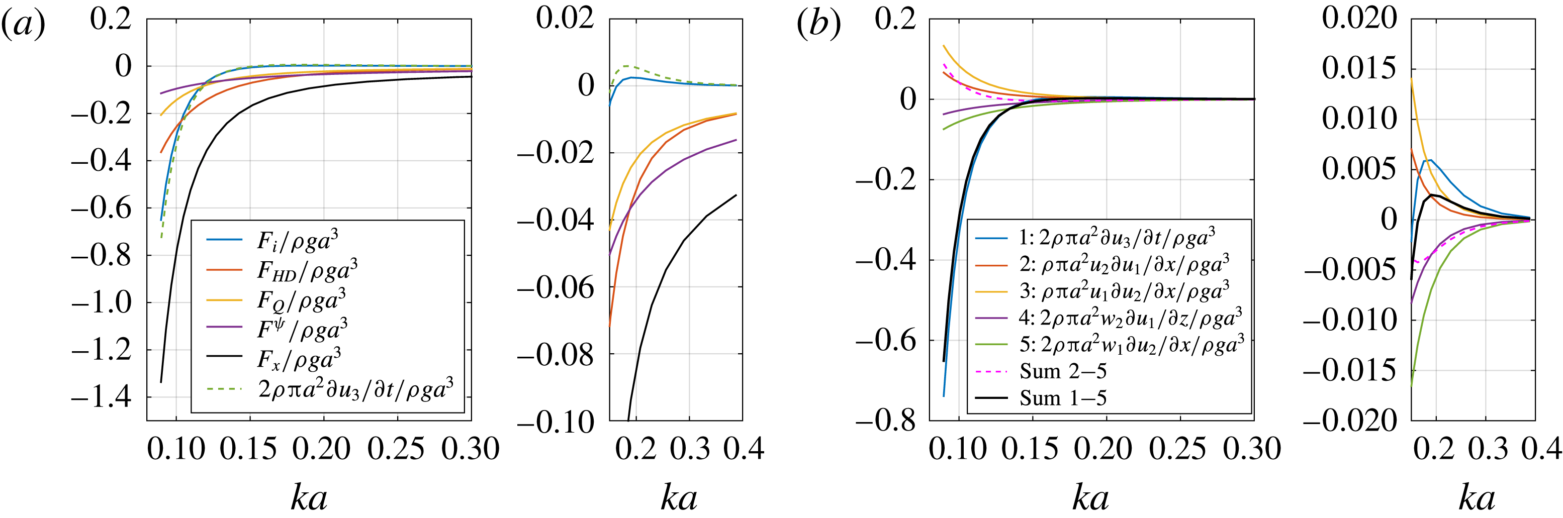
Illustrative example of force components of the third harmonic load in the generalized FNV model. Water depth
 $h/a=7.83$
. (a) Force components, where
 $F_{x}$
denotes the total force (2.7),
 $F_{i}=\int _{-h}^{0}F^{\prime }\,\text{d}z$
, with
 $F^{\prime }$
given by (2.2), while
 $F_{HD}$
,
 $F_{Q}$
and
 $F^{\unicode[STIX]{x1D6F9}}$
are defined by (2.7), (2.8) and (2.9) respectively. (b) Components of
 $F_{i}$
. It should be noted that, for circular cross-sections, the distributed force terms in Rainey’s model (equation (22) in Manners & Rainey Reference Manners and Rainey1992) agree with
 $F^{\prime }$
in the FNV model, given by (2.2). The only difference between the two load models is therefore the
 $F^{\unicode[STIX]{x1D713}}$
term.

2.4 Force term contributions to the
 $3\unicode[STIX]{x1D714}$
loads

An interesting question relates to the relative magnitudes of the different terms in the load formulation. This is illustrated for water depth
 $h/a=7.83$
in figure 2. The contributions to the third harmonic of the horizontal force from the terms in (2.7) are compared. The range of the horizontal axis spans from deep water to intermediate, or near shallow, water depth wave conditions. Due to the fact that there is no third-order wave radiation in the FNV method, all of the components are either 0 or
 $180^{\circ }$
apart. This is indicated by positive and negative sign of the quantities given in the figure.
An important observation is that the term due to the incoming third-order incident wave component,
 $\unicode[STIX]{x2202}u_{3}/\unicode[STIX]{x2202}t$
, becomes a major contributor in finite water depth. Another observation is that the
 $F^{\unicode[STIX]{x1D713}}$
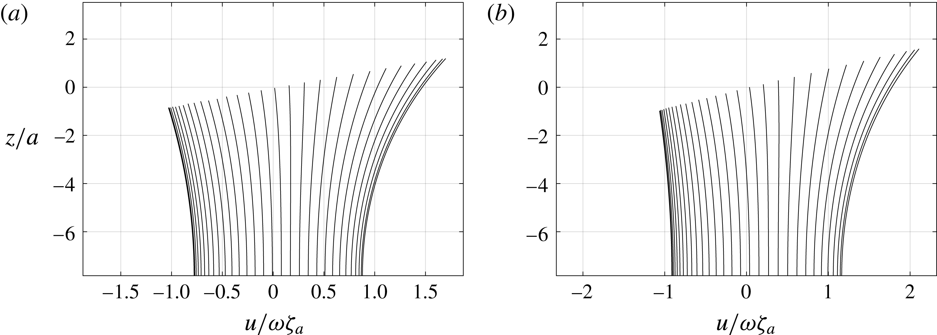
term, which accounts for half of the third harmonic force in deep water, contributes the least in intermediate water depth. It should be noted also that the horizontal advection terms provide larger-magnitude forces than the vertical ones, even though the latter are multiplied by a factor of 2, cf. (2.2). This is an effect of finite water depth; the horizontal velocities and accelerations are larger than the vertical ones. Two illustrative examples showing the horizontal velocity
 $u(z)$
as predicted by Stokes fifth-order wave theory at time steps
 $T/80$
over one wave period
 $T$
are provided in figure 3. The kinematics clearly deviates from that predicted by linear wave theory at this water depth. For later discussions related to flow separation, it should be noted that the magnitude of the horizontal velocity is clearly larger at the wave crest than at the wave trough.
Example of horizontal velocity
 $u$
at the cylinder axis according to fifth-order Stokes wave theory for two selected relevant regular wave conditions:
 $h/a=7.83$
, wave steepness
 $H_{1}/\unicode[STIX]{x1D706}=1/25$
,
 $ka=0.127$
(a) and
 $ka=0.105$
(b). Here,
 $\unicode[STIX]{x1D701}_{a}$
is the linear wave amplitude and
 $\unicode[STIX]{x1D714}=2\unicode[STIX]{x03C0}/T$
, with
 $T$
the wave period. The time step between each curve is
 $T/80$
. It should be noted that for
 $ka=0.105$
, the magnitude of the velocity is larger at the sea floor in the positive direction than at the free surface in the negative direction.

2.5 Direct numerical integration
A direct approach of evaluating the integral in (2.1) must be used in the case of, for instance, applying a numerical wave tank. In the present work, we present results both from the approach described in § 2.3 and from direct numerical integration. For the direct numerical integration approach, we integrate
 $F^{\prime }$
up to the instantaneous fifth-order incident free surface using Stokes fifth-order wave theory (see, for instance, the classical paper by Skjelbreia & Hendrickson (Reference Skjelbreia and Hendrickson1960)), and add the
 $F^{\unicode[STIX]{x1D713}}$
from (2.3). A misprint in their paper pointed out, for instance, by Fenton (Reference Fenton1985) should be noted: the sign ahead of the number 2592 in the expression of
 $C_{2}$
used in the fifth-order formula for the phase speed is wrong. Consistent with the derivation of the fifth-order Stokes wave theory, we use the following Taylor expansion to evaluate the quantities in (2.2) for
 $0\leqslant z\leqslant |\unicode[STIX]{x1D701}|$
:
 $$\begin{eqnarray}\displaystyle f(z) & = & \displaystyle (f_{1}+f_{2}+f_{3}+f_{4}+f_{5})+z\frac{\unicode[STIX]{x2202}(f_{1}+f_{2}+f_{3}+f_{4})}{\unicode[STIX]{x2202}z}\end{eqnarray}$$
 $$\begin{eqnarray}\displaystyle & & \displaystyle +\,\frac{z^{2}}{2}\frac{\unicode[STIX]{x2202}^{2}(f_{1}+f_{2}+f_{3})}{\unicode[STIX]{x2202}z^{2}}+\frac{z^{3}}{6}\frac{\unicode[STIX]{x2202}^{3}(f_{1}+f_{2})}{\unicode[STIX]{x2202}z^{3}}+\frac{z^{4}}{24}\frac{\unicode[STIX]{x2202}^{4}f_{1}}{\unicode[STIX]{x2202}z^{4}},\end{eqnarray}$$
where
 $f_{i}$
and derivatives of
 $f_{i}$
are evaluated at
 $z=0$
. As described above, a time series of
 $F_{x}$
is in turn constructed numerically and band-pass filtered to extract the harmonics.
This approach provides higher harmonic loads than
 $3\unicode[STIX]{x1D714}$
. It should be noted that the scattering potential is consistent to third order only, as in the original FNV method, and the inclusion of terms of higher order than three is only correctly expressed in the incident wave potential.
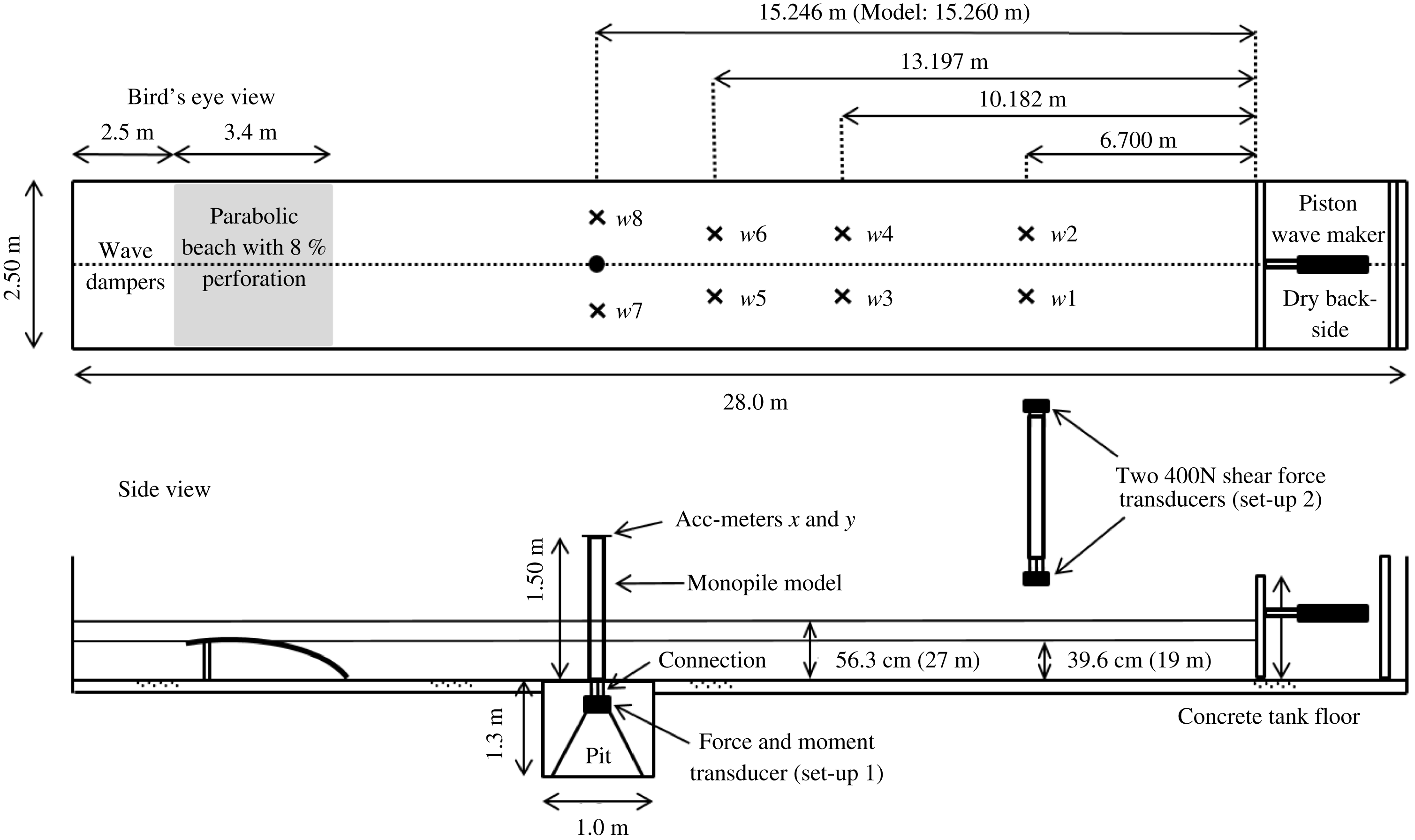
Model test set-up of the present experiments performed in a medium-size wave tank at the Marine Technology Centre, NTNU.

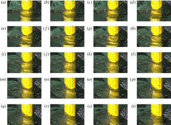
Snapshots from high-speed video with incident wave from right towards left. The time instants are approximately
 $T/80$
apart and are labelled sequentially from (a) to (t). Water depth
 $h/a=7.83~\text{m}$
,
 $ka=0.127$
,
 $H_{1}/\unicode[STIX]{x1D706}=1/25$
. At a model scale of
 $1:48$
, the water depth is
 $h=27~\text{m}$
, the cylinder radius
 $a=3.45~\text{m}$
, wave period
 $T=12~\text{s}$
, and the horizontal lines are 1 m apart (numbers given above their corresponding lines). The vertical lines are
 $30^{\circ }$
apart. The confetti was used for flow visualization. One should note in particular the local run-up at the rear of the model, which breaks laterally and forms a local upstream propagating wave.

3 Experiments
Dedicated experiments were carried out in a medium-size wave tank at the Marine Technology Centre, NTNU; see figure 4. The model diameter was 0.144 m. The ratio between the tank breadth and the model diameter was 17.4. The wave maker was of piston type. Both regular and irregular wave tests were conducted. Here, we consider regular wave tests only. An example of snapshots of the wave field near the cylinder obtained from high-speed video is provided in figure 5. A supplementary movie showing the sequence is provided at https://doi.org/10.1017/jfm.2017.702.
The tests were automated. The wave maker was programmed to run regular tests with a prescribed number of periods (typically 60), with pauses in between (2–5 min). In this manner, we were able to obtain a large number of tests. During one 24 h duration test, we typically obtained approximately 200 regular wave conditions, or 40 irregular wave conditions. There are clear advantages to this. The number of tests is increased, human error is decreased and the tests are consistent with one another, something that increases the quality of the data. The value of the data is further increased when one can readily perform repetition tests. Several thousand regular wave tests were carried out for the present study. Due to space limitations, only selected results are included, chosen so as to describe our main findings.
One main finding, which has already been mentioned in the Introduction, is that the third harmonics of the loads are well described by the generalized FNV theory for small to medium steepness waves, while there is a consistently increasing discrepancy for larger wave steepnesses.
3.1 Instrumentation
The measurements included the horizontal force
 $F_{x}$
and the overturning moment
 $M_{y}^{m}$
, free-surface elevations by wave gauges, wave maker motion and water temperature. High-speed video was taken, including attempts at flow visualization using confetti on the free surface (cf. the supplementary movie). The moment was measured at a position
 $z_{m}=-0.317~\text{m}$
below the tank floor (mudline). The mudline moment
 $M_{y}$
was calculated as
 $M_{y}=M_{y}^{m}+z_{m}F_{x}$
. The mean temperature varied between 13 and
 $17~^{\circ }\text{C}$
over the testing period. The wave gauge calibration factors increased by approximately
 $2\,\%/^{\circ }\text{C}$
. This was corrected for in the post-processing. The force and moment transducer was insensitive to temperature changes, and was found to be very stable in general. The testing took place during several phases with more than one year in between, but the calibration factor of the load sensor varied by less than 1 % over the whole period. This applies to force transducer set-up 1 (see figure 4); two load measuring set-ups were used, denoted as force transducer set-ups 1 and 2. The purpose of force transducer set-up 2 was to investigate the accuracy of the force transducer used in force transducer set-up 1. In force transducer set-up 1, the horizontal force and moment were measured with a commercially available seismic shear force transducer, modified by MARINTEK to also measure the moment. The range of the force transducer was 7500 N, which was two to three orders of magnitude higher than needed for the typical loads in the present tests. Its high stiffness was necessary in order to obtain an adequately high natural frequency of the set-up. The wet natural frequency of the set-up was 23 Hz. The accelerometers at the top of the model were used to check that the cylinder vibrations were negligible. In force transducer set-up 2, 2
 $\times$
400 N shear force transducers from MARINTEK were used, one at the top and one at the bottom of the model. The natural frequency was 30 Hz. The model was clamped onto the transducers, so that moments were not obtained in this set-up. There was clearly less measurement noise in the force signals obtained in force transducer set-up 2, but the main trends of the load harmonics were practically identical to those obtained in force transducer set-up 1 (figure 15).
3.2 Test conditions
One single monopile model was tested in two water depths,
 $h/a=7.83$
and
 $h/a=5.51$
. The waves ranged from deep to intermediate depth wave conditions. Our main focus was on relatively long and moderately steep to considerably steep waves up to the breaking limit. The reason is that we observed consistent discrepancies with the theoretical third harmonic of the loads for steep wave conditions.
At an imagined model scale of
 $1:48$
, the diameter of the monopile is
 $D=6.9~\text{m}$
, the two water depths are
 $h=27~\text{m}$
and 19 m and the wave periods are between
 $T=6~\text{s}$
and 16.5 s by Froude scaling.
The wave steepness
 $H_{1}/\unicode[STIX]{x1D706}$
ranged from
 $1/140$
to
 $1/16$
, where
 $H_{1}$
is the linear wave height. By linear wave height,
 $H_{1}$
, we refer to the following. For small-amplitude waves, the wave maker motion was prescribed according to linear wave maker theory. Except for rather minor modifications of the wave maker motion by use of a mechanical transfer function, good agreement between the measurements and the theory was achieved for small-amplitude waves, say for
 $H_{1}/\unicode[STIX]{x1D706}<1/50$
. When generating waves with higher steepness, the wave maker motion was simply scaled linearly. This means that the first harmonic in the measured wave does not correspond exactly to
 $H_{1}$
as used herein; it is somewhat smaller. This effect is, however, not dominant, and we use the term
 $H_{1}/\unicode[STIX]{x1D706}$
to characterize the wave conditions throughout the paper.
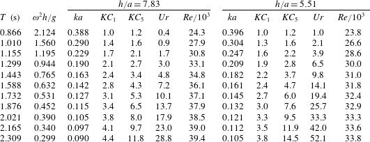
Test condition parameters. The leftmost column provides the (model scale) wave periods in the present model tests. The Keulegan–Carpenter numbers (
 $KC$
), Ursell numbers (
 $Ur$
) and Reynolds numbers (
 $Re$
) are given for a wave steepness
 $H_{1}/\unicode[STIX]{x1D706}=1/25$
.
 $KC_{1}$
and
 $KC_{5}$
refer to the maximum wave particle velocity at the wave crest according to linear and fifth-order Stokes theory respectively.

Selected descriptive parameters are provided in table 1. The Keulegan–Carpenter numbers are given by
 $$\begin{eqnarray}\displaystyle KC_{1}=\frac{U_{m1}T}{D}=\unicode[STIX]{x03C0}\frac{H_{1}}{D},\quad KC_{5}=\frac{U_{m5}T}{D}, & & \displaystyle\end{eqnarray}$$
where
 $T=2\unicode[STIX]{x03C0}/\unicode[STIX]{x1D714}$
is the wave period,
 $U_{m1}=\unicode[STIX]{x1D714}\unicode[STIX]{x1D701}_{a}/\text{tanh}\,kh$
is the amplitude of the horizontal velocity at
 $z=0$
as predicted by linear wave theory and
 $U_{m5}$
is the maximum horizontal velocity at the incident wave crest according to fifth-order Stokes theory. In the table, the numbers are given for wave steepness
 $H_{1}/\unicode[STIX]{x1D706}=1/25$
.
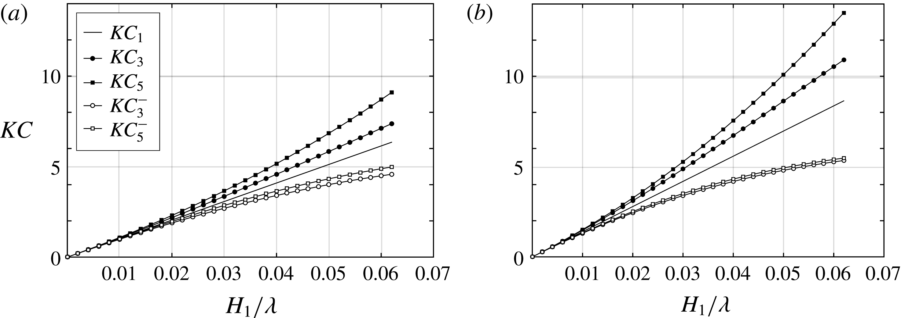
The different Keulegan–Carpenter numbers are illustrated for two relevant wave conditions in figure 6. In the quantities with minus sign as superscript, the maximum velocity in the opposite direction to the wave-propagation direction is used, that is, the horizontal velocity at the incident free surface during a wave trough. Since the effect of flow separation increases with
 $KC$
, this figure illustrates clearly that flow separation effects are expected to be most prominent in the direction of the wave propagation.
Example illustrating different
 $KC$
numbers for wave steepness
 $H_{1}/\unicode[STIX]{x1D706}$
ranging from 0 to
 $1/16$
at water depth
 $h/a=7.83$
, for
 $ka=0.127$
(a) and
 $ka=0.105$
(b). Here,
 $KC_{n}$
means that the horizontal velocity in the incident wave at the wave crest according to
 $n$
th-order Stokes theory is used. A minus sign as superscript indicates that the velocity at the wave trough is used.

The wavenumber
 $k$
in
 $KC_{1}$
and
 $H_{1}/\unicode[STIX]{x1D706}$
is taken to be that from the linear dispersion relationship. In
 $KC_{3}$
and
 $KC_{5}$
, the dispersion relationship is corrected to third order (cf., for instance, Skjelbreia & Hendrickson Reference Skjelbreia and Hendrickson1960).
The wave height in the Ursell number,
 $Ur$
, is taken as the linear wave height,
 $H_{1}$
, which is in accordance with the original paper by Ursell (Reference Ursell1963),
 $$\begin{eqnarray}\displaystyle Ur=\frac{H_{1}\unicode[STIX]{x1D706}^{2}}{h^{3}}. & & \displaystyle\end{eqnarray}$$
The Reynolds number is given by
 $$\begin{eqnarray}\displaystyle Re=\frac{U_{m1}D}{\unicode[STIX]{x1D708}}. & & \displaystyle\end{eqnarray}$$
Here,
 $\unicode[STIX]{x1D708}=10^{-6}~\text{m}^{2}~\text{s}^{-1}$
is used as the kinematic viscosity of water, which neglects small variations due to the temperature of fresh water. The Reynolds numbers in the tests suggest laminar boundary layers, which implies a problem when flow separation occurs and the results are scaled to prototype conditions with turbulent boundary layer flow. The reasons are that the flow separation line is affected by the boundary layer condition, and flow separation influences pressure loads. Since viscous stresses do not have important contributions to the hydrodynamic force and moments on the cylinder, the state of the boundary layer is less important with no flow separation.
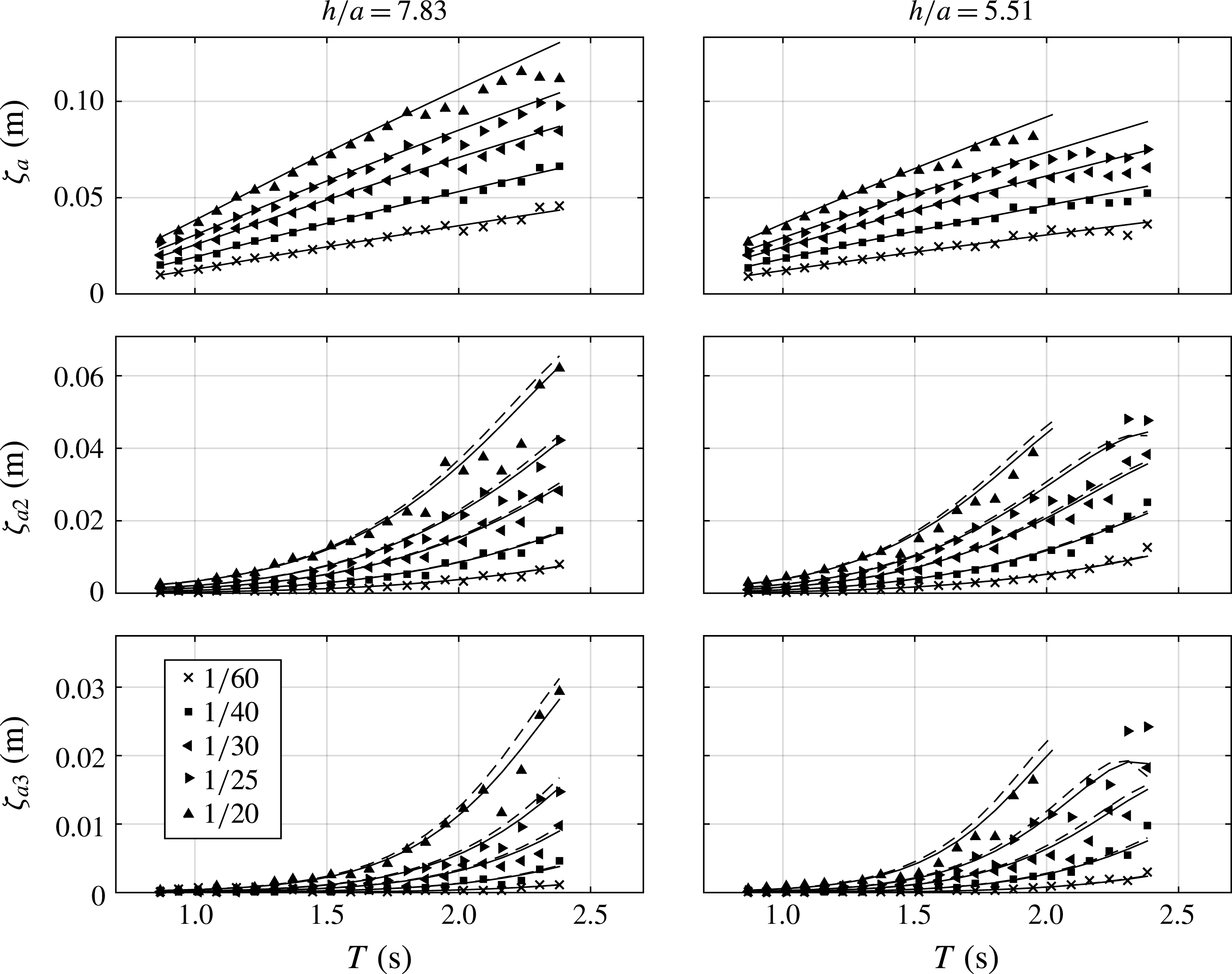
Amplitudes of the first three regular wave harmonics (model scale) measured at model position
 $w8$
(cf. figure 4) from selected wave calibration tests versus the wave period
 $T$
. The numbers in the legend refer to the wave steepness
 $H_{1}/\unicode[STIX]{x1D706}$
. Markers: experiments. The solid and dashed curves indicate that
 $k$
is calculated from the linear (dashed) and third-order (solid) dispersion relationships respectively (
 $\unicode[STIX]{x1D701}_{a}=H_{1}/2$
in both cases).

A representative set of the regular wave conditions tested in the present study plotted in an
 $H/h$
versus
 $\unicode[STIX]{x1D706}/h$
diagram, as suggested by Fenton (Reference Fenton1990). Grey markers: waves broke along the tank. Black markers: the three wave periods where detailed data are provided. (a) Water depth
 $h/a=5.51$
; (b) water depth
 $h/a=7.83$
.

3.3 Calibrated waves
The wave gauges were calibrated to have an error within 1 %–2 %. Wave calibration tests without the model were run for a representative range of waves. The amplitudes of the harmonics were extracted using a narrow-band filter based on the fast Fourier transform. The amplitudes of the first three wave harmonics for selected conditions, measured at the model position
 $w8$
(cf. figure 4), are provided in figure 7. The agreement between theory and experiments is fair.
There are oscillating types of deviations from the theory. We believe that there are two main causes: wave reflections from the beach and parasitic waves generated by the wave maker. There are also other uncertainties related to wave tests in a closed tank, such as, for instance, seiching, transverse waves and mechanical noise of the wave maker.
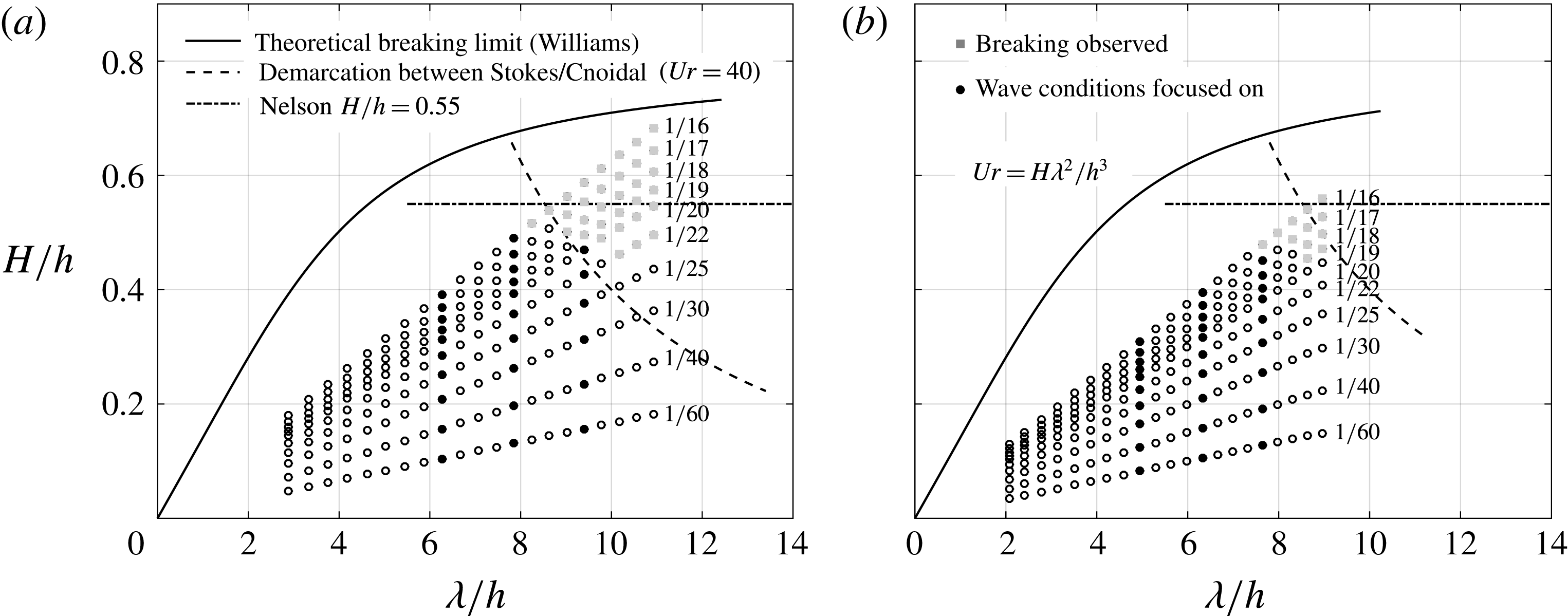
The longest and most nonlinear waves broke just after the wave maker. The waves that broke are indicated by grey markers in figure 8, where a representative set of the presently tested regular wave conditions are plotted in a chart suggested by Fenton (Reference Fenton1990); an Ursell number of 40 (dashed curve) is suggested to provide an upper limit for fifth-order Stokes theory be valid. Above this limit, he recommends using cnoidal wave theory. We see from figure 8 that basically all of the presently considered non-breaking wave conditions are within the Stokes fifth-order wave theory regime, and in particular the three wavenumbers that are focused on in the results section (black markers). The curve
 $H/h=0.55$
was suggested by Nelson (Reference Nelson1994) to be an upper practical limit before wave breaking in a very flat bottomed wave tank.
3.3.1 Beach reflections
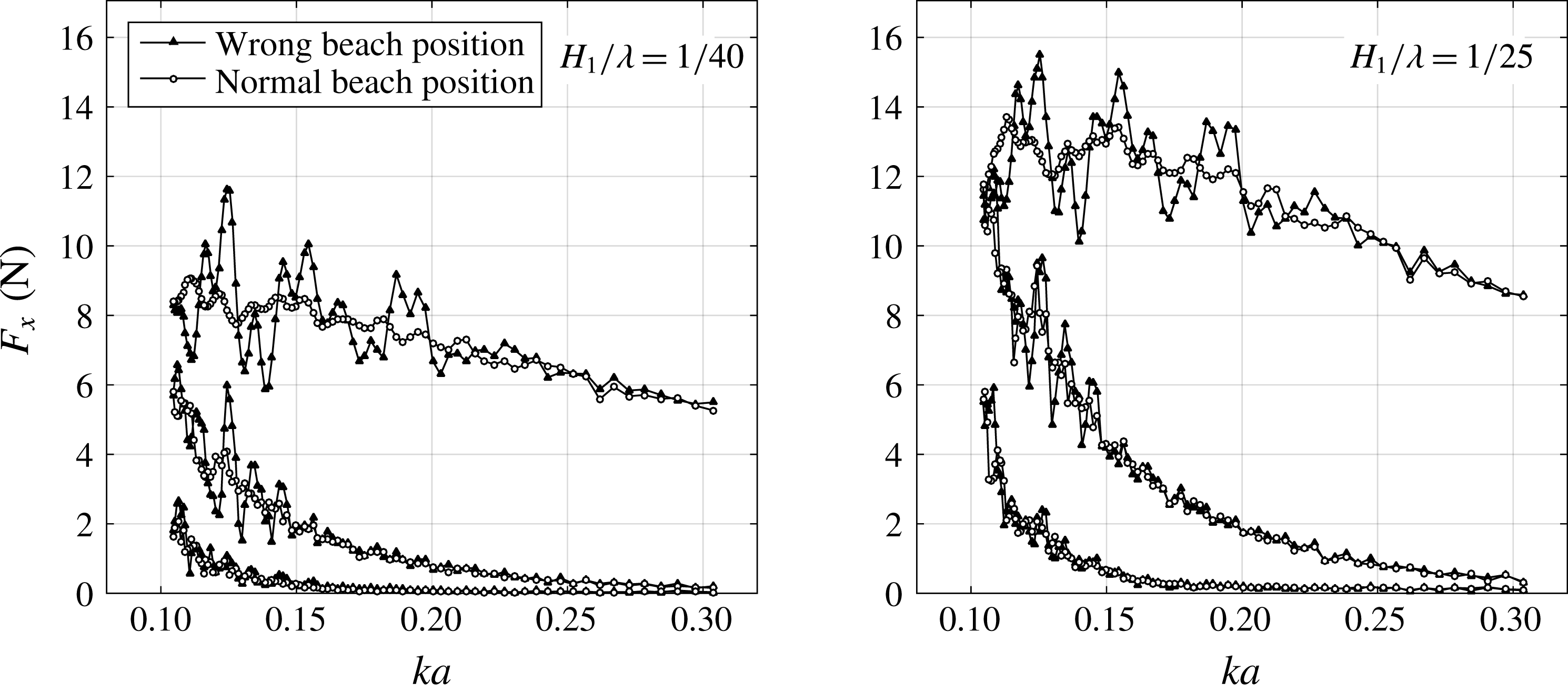
The wave reflections from the beach are most pronounced for wavelengths that are of equal length or longer than the beach. The reflections cause an oscillatory nature of the reduced data as a function of the non-dimensional wavenumber
 $ka$
. This is illustrated in figure 9, where the effect of an (erroneous) extreme beach height on the horizontal force is illustrated. By beach height we mean the height of the uppermost point of the beach, relative to still water. The beach height in the test was 1.5 cm (referred to as ‘normal’ in the legend). The results in figure 9 show that the reflection level is reasonably low for waves that are shorter than the beach. Based on observing the deviations in the data from a curve fit (not shown), the relative error is estimated to be of the order of 2 %–3 %.
Illustration of beach reflection effects on the first three harmonics of the horizontal force
 $F_{x}$
versus non-dimensional wavenumber
 $ka$
. The parabolic beach was normally placed with its top position 1.5 cm above the still water line; in the tests denoted as ‘Wrong beach position’, this value was 18 cm.
 $H_{1}/\unicode[STIX]{x1D706}=1/25$
; water depth
 $h/a=5.51$
.

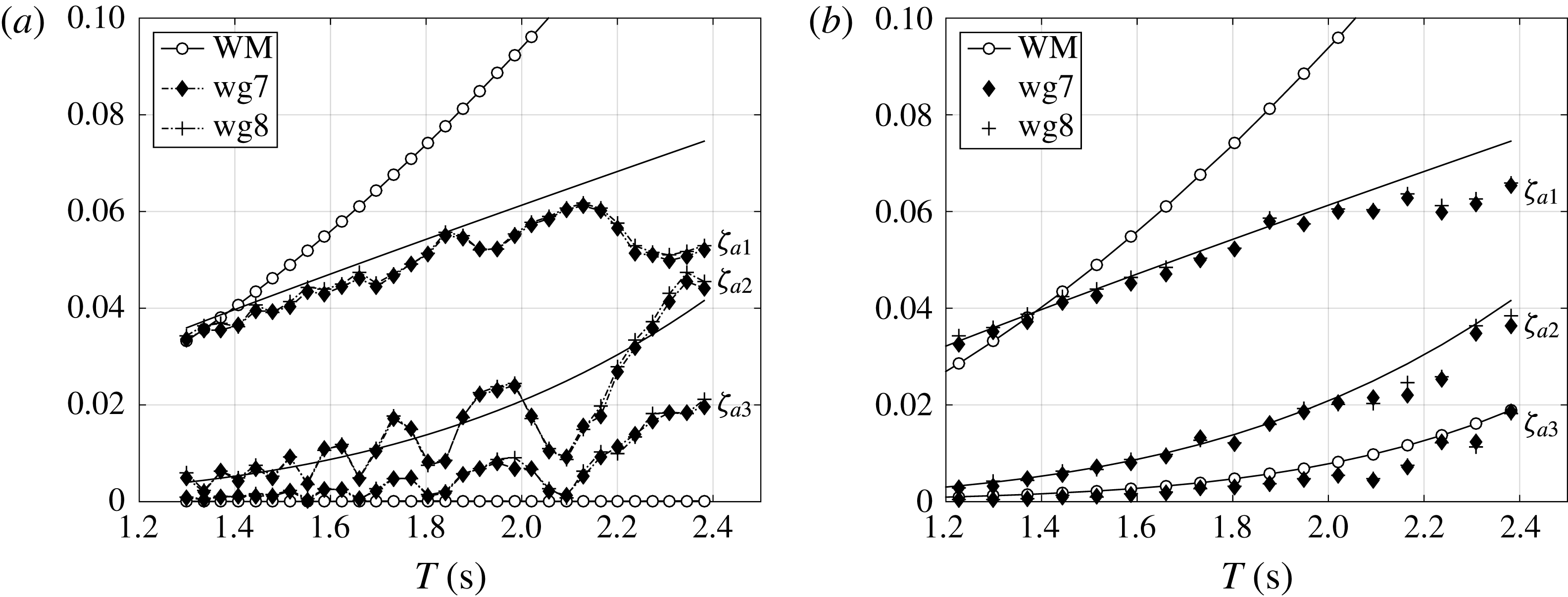
Illustration of parasitic wave occurrence and reduction in the experiments. The amplitudes of the first three harmonics of the measured waves at wg7 and wg8 in wave calibration tests (cf. figure 4) and the amplitude of the measured wave maker motion, denoted by WM (only first and second harmonics of WM shown), versus wave period
 $T$
. Wave steepness
 $H_{1}/\unicode[STIX]{x1D706}=1/30$
and water depth
 $h/a=5.51$
. (a) The motion of the wave maker contains
 $\unicode[STIX]{x1D714}$
signal only. (b) The
 $2\unicode[STIX]{x1D714}$
component of the wave maker motion has been added to reduce the parasitic second-order waves.

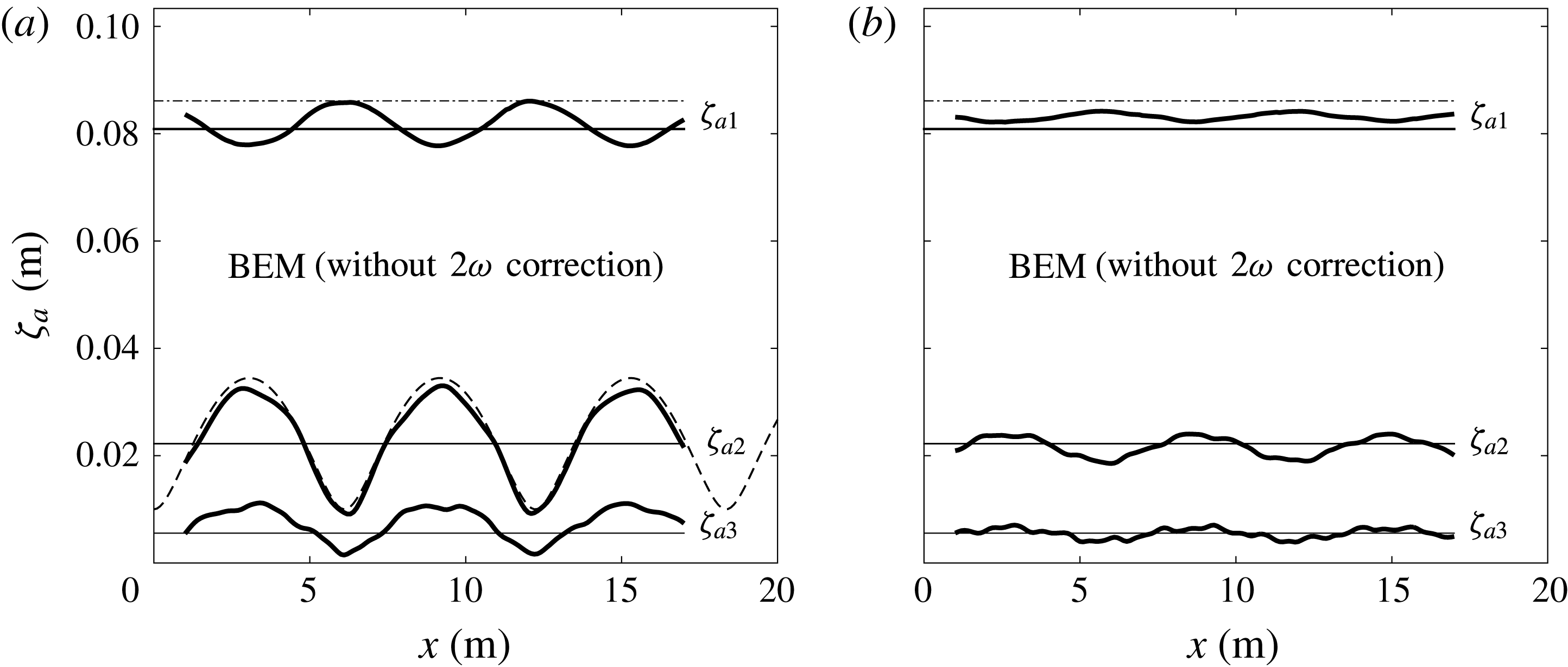
Examples of wave amplitude versus distance
 $x$
from the wave maker from simulations using a fully nonlinear 2D numerical wave tank based on a Rankine type boundary element method (BEM), compared with Stokes wave theory. (a) Without
 $2\unicode[STIX]{x1D714}$
parasitic wave correction of the wave maker signal. (b) With
 $2\unicode[STIX]{x1D714}$
correction signal (amplitude
 $\unicode[STIX]{x1D701}_{2p}=0.55\unicode[STIX]{x1D701}_{a2}$
based on observation). Dash-dot curve:
 $\unicode[STIX]{x1D701}_{a1}$
as predicted by linear wave theory. Solid horizontal curves: amplitudes
 $\unicode[STIX]{x1D701}_{a1}$
,
 $\unicode[STIX]{x1D701}_{a2}$
,
 $\unicode[STIX]{x1D701}_{a3}$
predicted by Stokes fifth-order wave theory. Dashed curve: theoretical amplitude of second harmonic along the tank due to interference between bound and parasitic waves with amplitude
 $\unicode[STIX]{x1D701}_{p2}=0.55\unicode[STIX]{x1D701}_{a2}$
. Water depth
 $h/a=7.83$
,
 $ka=0.105$
,
 $H_{1}/\unicode[STIX]{x1D706}=1/25$
.

3.3.2 Parasitic waves
Parasitic waves were investigated in some detail. Parasitic waves are free (unwanted) waves generated by the wave maker, or by the tank topology. The latter effect is not relevant in the case of constant water depth as in the present study. In all of our tests, due to the finite water depth conditions, there was no available time window prior to the arrival of second-order parasitic waves, as utilized, for instance, by Huseby & Grue (Reference Huseby and Grue2000). Parasitic waves were therefore reduced by adding a
 $2\unicode[STIX]{x1D714}$
signal to the wave maker motion.
One can write the total signal of the free surface to second order, including the (free) second harmonic parasitic wave component as
 $$\begin{eqnarray}\displaystyle \unicode[STIX]{x1D701}=\unicode[STIX]{x1D701}_{a}\sin (\unicode[STIX]{x1D714}t-kx)+\unicode[STIX]{x1D701}_{2a}\sin (2\unicode[STIX]{x1D714}t-2kx)-\unicode[STIX]{x1D701}_{2p}\sin (2\unicode[STIX]{x1D714}t-k_{2}x), & & \displaystyle\end{eqnarray}$$
where
 $k_{2}$
obeys
 $(2\unicode[STIX]{x1D714})^{2}=gk_{2}\tanh k_{2}h$
,
 $\unicode[STIX]{x1D701}_{2a}$
is the amplitude of the bound second harmonic component according to Stokes wave theory and
 $\unicode[STIX]{x1D701}_{2p}$
is the amplitude of the second-order parasitic wave. The magnitude was determined empirically as
 $\unicode[STIX]{x1D701}_{2p}=0.55\unicode[STIX]{x1D701}_{2a}$
, based on the results exemplified in figure 10(a). The second-order parasitic waves give rise to an oscillatory nature of the wave harmonic amplitude as a function of
 $T$
, as expected, based on (3.4). The phase between the bound and parasitic free
 $2\unicode[STIX]{x1D714}$
components is
 $\unicode[STIX]{x03C0}$
at the mean wave maker position, independent of the wave frequency (cf. Hughes Reference Hughes1993). An alternative could be to use second-order wave maker theory, as, for instance, described by Schäffer (Reference Schäffer1996).
It is also evident that the second-order parasitic waves influence the first and third harmonics, in particular the latter. With the
 $2\unicode[STIX]{x1D714}$
correction signal of the wave maker motion, the third harmonic of the waves behaves significantly better as a function of
 $T$
; see figure 10(b). There are still irregularities associated with the fact that the parasitic second-order wave is not totally eliminated. Wave reflection from the beach is a further candidate that may have contributed to the irregularities. Still, the main trends are acceptable.
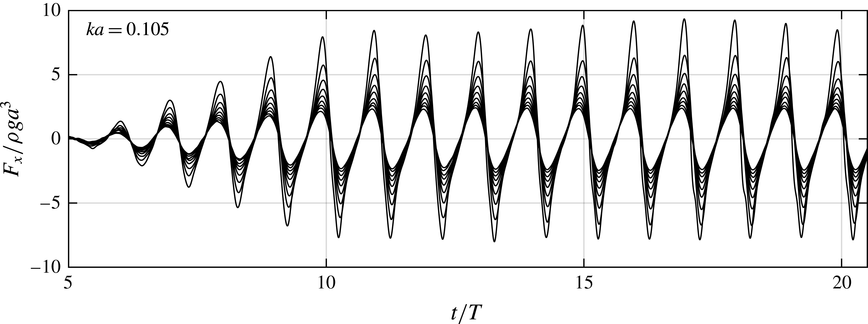
Experimental time series of normalized horizontal force (low-pass filtered at 5 Hz) for nine wave steepnesses:
 $H_{1}/\unicode[STIX]{x1D706}=1/60,1/55,1/50,1/45,1/40,1/35,1/30,1/25,1/20$
. Wavenumber
 $ka=0.105$
; water depth
 $h/a=7.83$
.

The existence of third-order parasitic waves is also exemplified in figure 11. Here, results from simulations with a 2D fully nonlinear wave tank based on the boundary element method (BEM) (cf. Kristiansen Reference Kristiansen2009) are presented. The first three harmonics of the wave are presented as functions of the spatial coordinate along the tank. Addition of the correction signal gives a clear improvement for the second-order parasitic waves, consistent with the experiments. The same oscillatory features are clearly seen in other studies where results from simulations of fully nonlinear wave tanks are compared with experimental data; see, for instance, Shao & Faltinsen (Reference Shao and Faltinsen2014).
3.3.3 Wave breaking
The longest and steepest waves broke along the tank. In figure 8, a representative selection of the present regular wave conditions are indicated by markers in the classical chart by Fenton (Reference Fenton1990). This provides an indication of the validity range of different wave theories as well as breaking limits. For instance, at water depth
 $h/a=7.83$
, only the highest steepness wave tested (
 $H_{1}/\unicode[STIX]{x1D706}=1/16$
) broke for
 $ka=0.105$
. This condition is inside the cnoidal wave theory region, and close to the breaking limit. For
 $h/a=5.51$
, the waves with
 $ka\leqslant 0.121$
broke for steepness
 $H_{1}/\unicode[STIX]{x1D706}>1/20$
in the present experiments. This is also inside the cnoidal wave theory region. A dedicated wave maker motion would be needed to allow for non-breaking waves at this degree of nonlinearity. We note from the figure that most of our conditions correspond to intermediate water depth waves, while no conditions correspond to shallow water waves.
3.4 Force and moment time series
Examples of time series of normalized experimental horizontal force are provided in figure 12. The wave condition
 $h/a=7.83$
,
 $ka=0.105$
is considered at nine wave steepnesses
 $H_{1}/\unicode[STIX]{x1D706}$
ranging from
 $1/60$
up to
 $1/20$
. The signals are low-pass filtered at 5 Hz to remove measurement noise. A linear ramp lasting for five wave periods was used when generating the waves. Except for the
 $1/20$
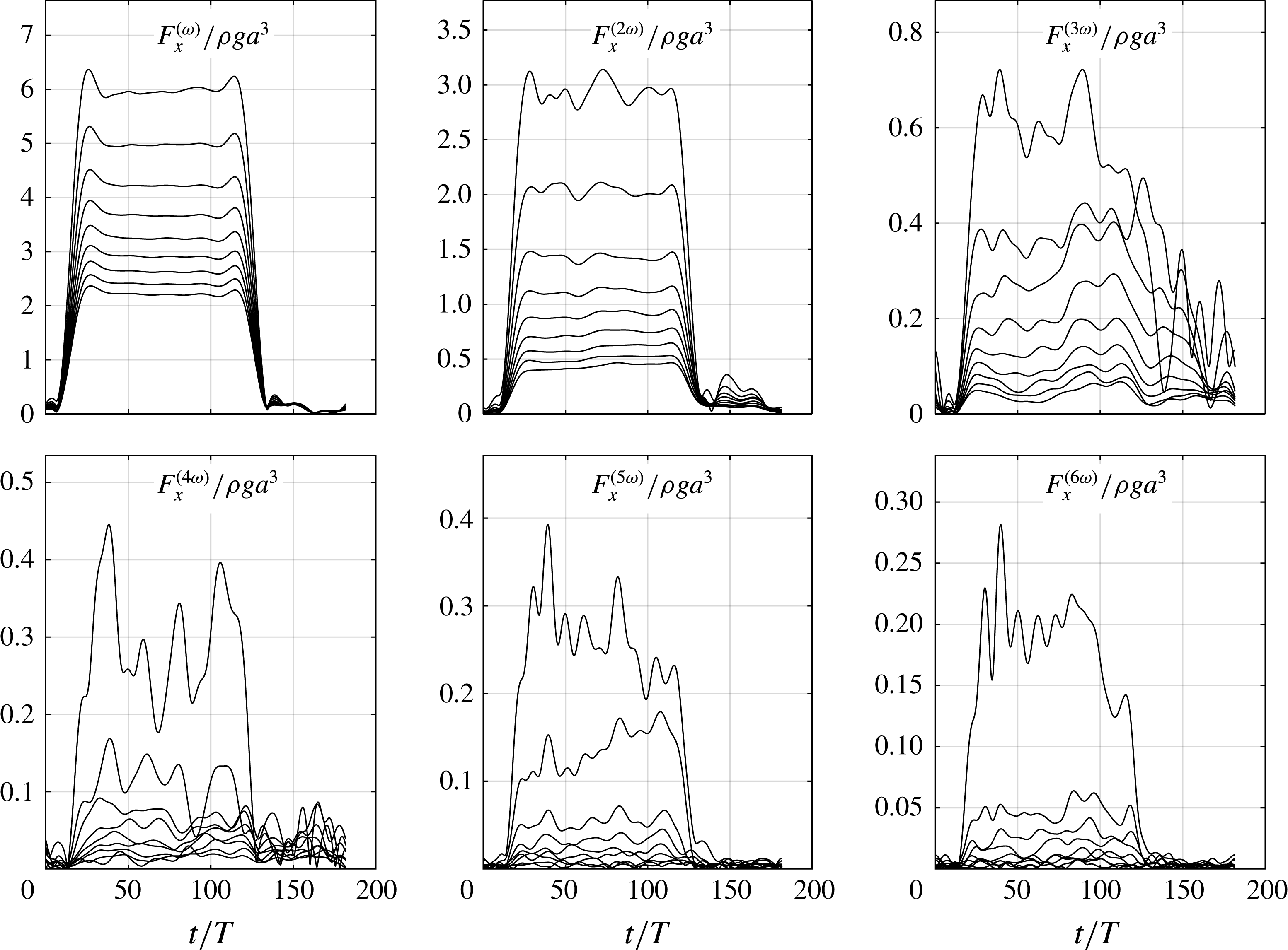
wave steepness case, the total time series are reasonably steady after the ramp-up period. There are more irregularities in the time series of each harmonic. These are obtained by narrow-band filters around each frequency. Examples including the first six harmonics are provided in figure 13. For clarity, the Hilbert envelopes, rather than time series, are displayed. The first and second harmonics are rather steady, while the third and higher harmonic signals display appreciable variations. There remain further studies to fully understand the irregularities. Possible explanations are parasitic waves, beach and side-wall reflections, as discussed above. Several time windows were used when extracting reduced data.
Hilbert envelopes of the first six harmonics of the normalized horizontal force
 $F_{x}/\unicode[STIX]{x1D70C}ga^{3}$
for nine wave steepnesses:
 $H_{1}/\unicode[STIX]{x1D706}=1/60$
,
 $1/55$
,
 $1/50$
,
 $1/45$
,
 $1/40$
,
 $1/35$
,
 $1/30$
,
 $1/25$
and
 $1/20$
. Same case as in figure 12 (
 $h/a=7.83$
,
 $ka=0.105$
).

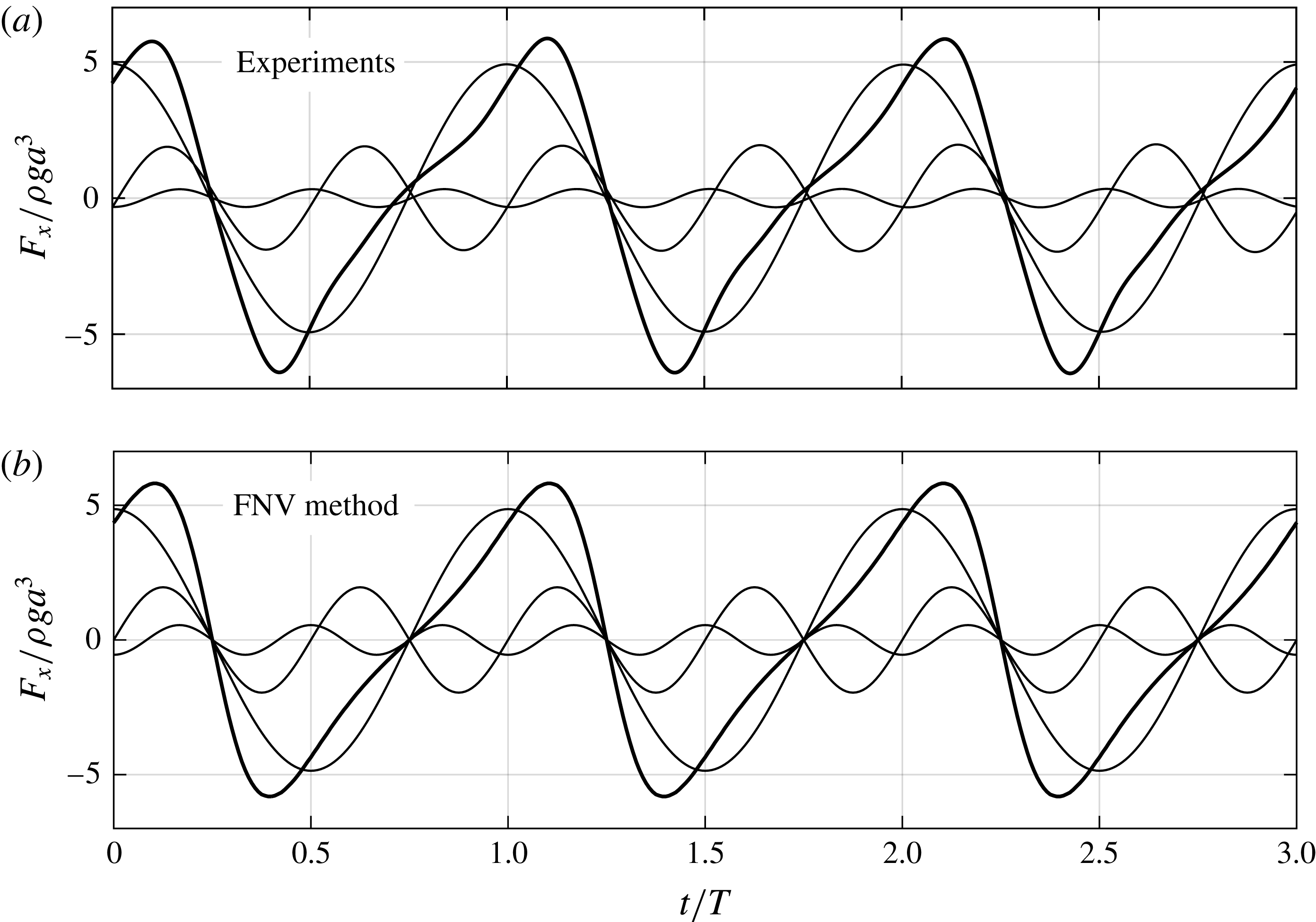
Example of time series of the total and first three harmonics of the normalized horizontal force. The time series of each harmonic is obtained by narrow band-pass filtering. (a) Experiments. (b) The generalized FNV method with wave kinematics integrated to the fifth-order free surface. It should be noted that the magnitude of the third harmonic is not in agreement, but the phase is in good agreement;
 $ka=0.105$
,
 $H_{1}/\unicode[STIX]{x1D706}=1/25$
, water depth
 $h/a=7.83$
.

4 Results
Results are presented, first by means of time-series examples, then in terms of reduced data; amplitudes of the harmonics of forces
 $F_{x}$
and moments
 $M_{y}$
. Only selected data are presented due to space limitations. The selection is considered to provide a suitable overview of the main findings.
4.1 Time-series examples
A representative example of time series of the total horizontal force and its first three harmonics is presented in figure 14, showing comparisons between experiments and the generalized FNV theory. The maxima of the time series of the first harmonic have been used to synchronize the two plots visually. There is, in general, a good overall agreement between the experiments and the theory, regarding both phases and amplitudes of the load harmonics. It should be noted in particular that the phase of the third harmonic agrees well. Several authors have indicated that the phasing of the third-order FNV load is not correct. In Huseby & Grue (Reference Huseby and Grue2000), deep water wave conditions were studied, and the FNV phase of the third harmonic force predicted by the FNV theory was up to
 $180^{\circ }$
out of phase with the experiments, depending on
 $ka$
(see figures 11b, 12b, 13b, 14b and 15b therein). The only notable discrepancy in the present study, which is for finite water depth conditions, is that the amplitude of the third harmonic is overestimated by the theory. This is the general trend in our results for large-steepness waves, something that will have the main focus in the remaining discussions.
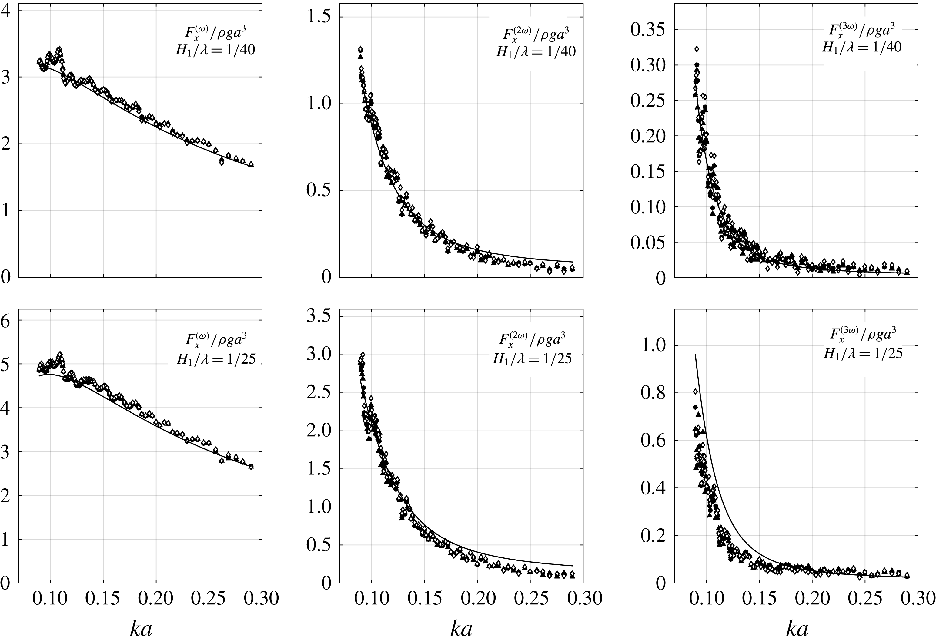
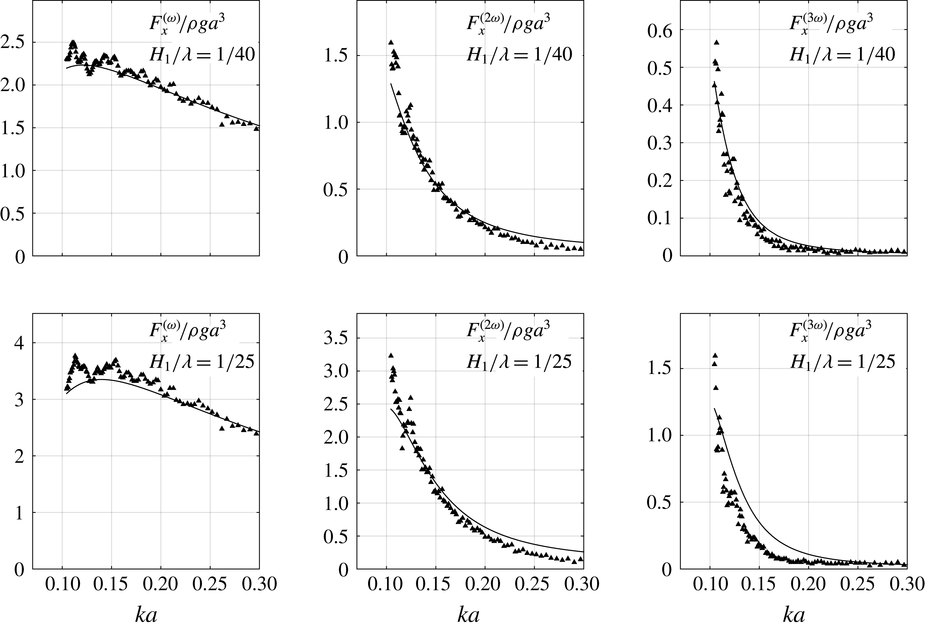
Horizontal force amplitude of the first three harmonics due to regular waves versus the non-dimensional wavenumber
 $ka$
for wave steepnesses
 $1/40$
and
 $1/25$
. The harmonics are indicated by superscripts. Water depth
 $h/a=7.83$
. Solid curves: generalized FNV theory. Triangles: force transducer set-up 1 with 120 s pause between each test. Circles: force transducer set-up 1 with 300 s pause. White diamonds: force transducer set-up 2 with 300 s pause. FNV theory: kinematics according to fifth-order Stokes theory applied to the incident fifth-order free-surface elevation.

4.2 Reduced data
The amplitudes of the first three harmonics of the horizontal force,
 $F_{x}$
, for two selected wave steepnesses are provided in figure 15. The present experimental data are compared with the generalized FNV theory. The water depth is
 $h/a=7.83$
. There are three sets of experimental results: the black triangles and circles represent results from tests with force transducer set-up 1, while the white diamonds represent results from force transducer set-up 2. The difference between the two force transducer set-ups is that a single 7500 N force transducer at the bottom of the model was used for set-up 1 (modified to also measure moments), while two
 $400~\text{N}$
force transducers were used in set-up 2 (one at the top and one at the bottom of the model).
In the tests represented by the triangles, the waiting time between each test was 120 s, while in the other two, it was 300 s. Although there is an oscillatory type of scatter of the data, the main trends are basically identical for both force transducer set-ups. This indicates that the results are not a function of the force transducers, or their set-up. Furthermore, although some of the individual data points are affected by the waiting time between tests (120 s or 300 s), the main trends are not. Different time windows for extracting the amplitudes were also investigated (cf., for instance, figure 13), with the same conclusions; some differences in the individual tests were observed, but the main trends were not affected. With reference to figure 9, it is argued that the oscillatory type of scatter in the first harmonic is mainly caused by beach reflections. The magnitude of the oscillatory type of scatter increases with higher harmonics. In addition, for the third harmonic, the scatter is highest for the smallest wave steepness (
 $H_{1}/\unicode[STIX]{x1D706}=1/40$
) and shortest waves. One should keep in mind that the absolute values of the third-order force components were small in the model tests.
It is clear that the first harmonic of the load is well described by the theory. This may be expected due to the high wavelength-to-model diameter ratio and the present
 $KC$
number range. Next, the agreement is good also for the second harmonic for
 $ka<0.12{-}0.15$
, while the theory overpredicts for shorter waves. The discrepancy increases gradually with increasing values of
 $ka$
. This is also as expected, since second-order wave scattering is not included in the FNV theory. Third, and perhaps most striking, is the level of overall agreement between theory and experiments for the third harmonic at the lowest wave steepness (
 $H_{1}/\unicode[STIX]{x1D706}=1/40$
). This applies for all of the wavelengths.
Example of the amplitude of the third harmonic of the horizontal force as a function of the wave steepness;
 $ka=0.105$
, water depth
 $h/a=7.83$
. Solid curve: generalized FNV theory. Diamond markers: data from present experiments.

Amplitudes of the first three harmonics of the horizontal force due to regular waves at water depth
 $h/a=7.83$
versus wave steepness for three non-dimensional wavenumbers
 $ka$
. Superscripts indicate harmonics.

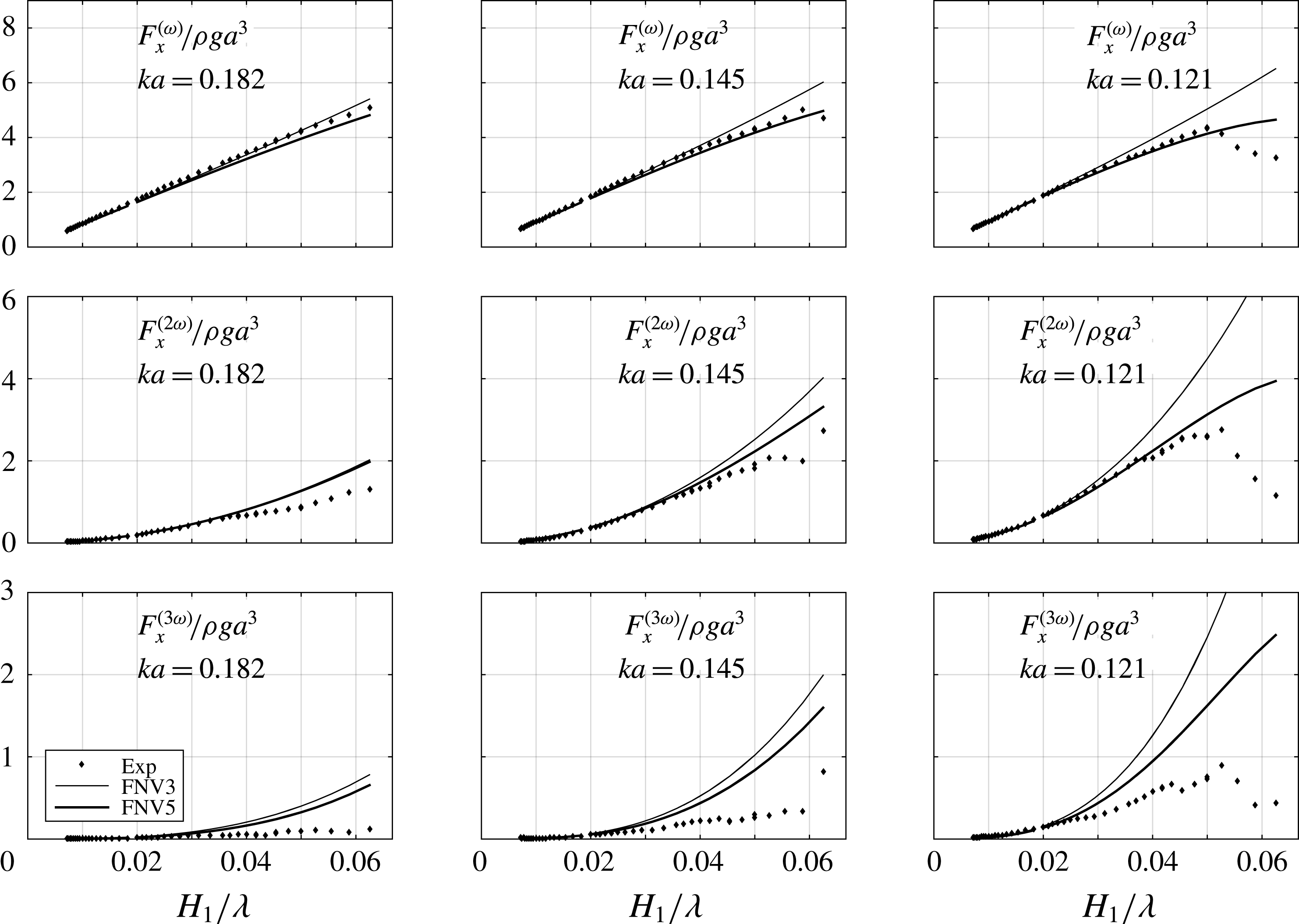
The theory, in general, overpredicts for the higher wave steepness,
 $H_{1}/\unicode[STIX]{x1D706}=1/25$
for
 $ka<0.18$
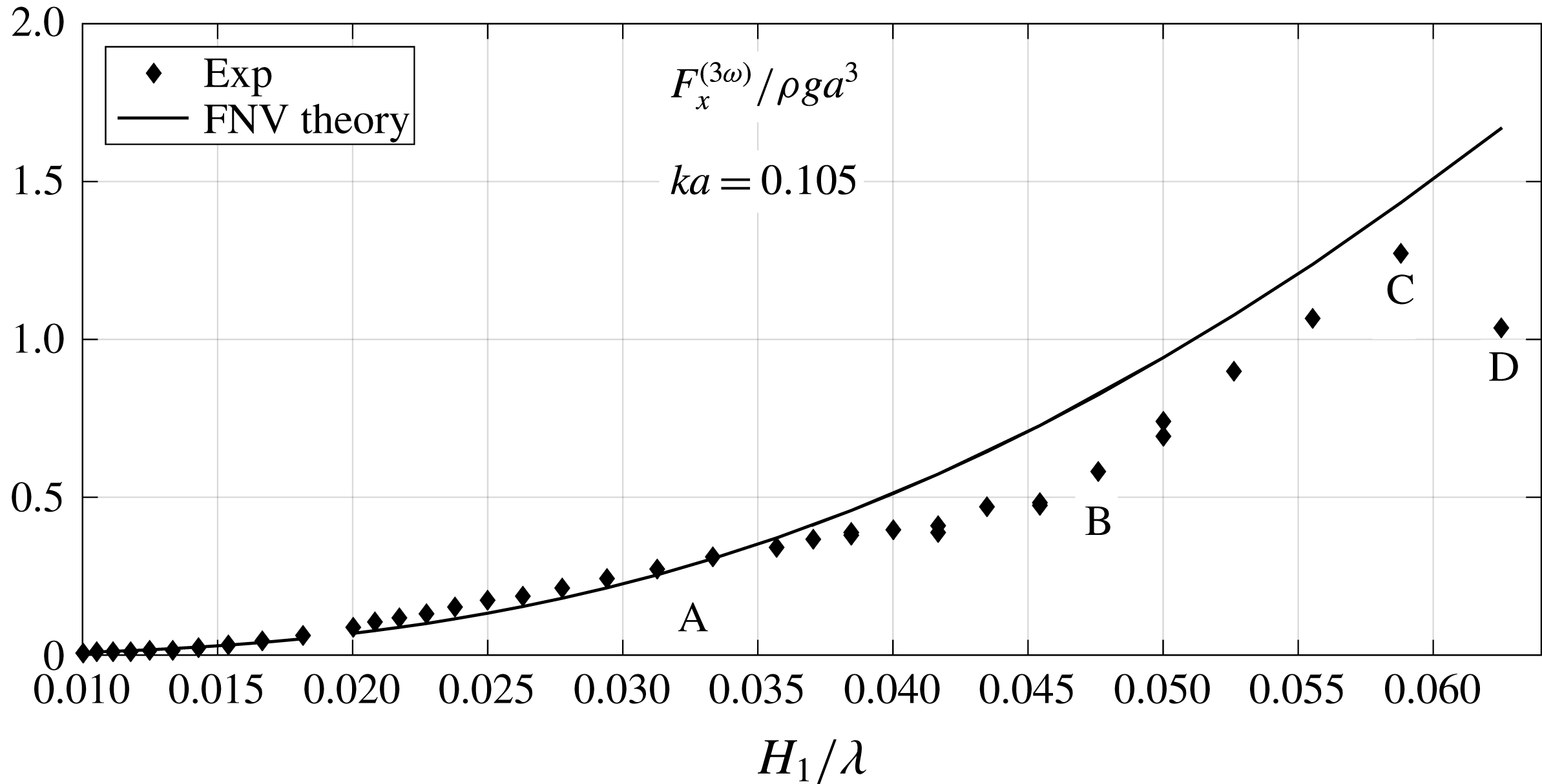
. This illustrates a general trend in our results for the third harmonic: the agreement is reasonable for small to medium wave steepness, while there is, in general, a monotonically increasing discrepancy with increasing steepness waves above this limit. This is exemplified in figure 16. Here, the amplitudes of the third harmonic of the horizontal force are presented as a function of wave steepness for a selected wave condition (
 $ka=0.105$
,
 $h/a=7.83$
). The main point in the figure is that the agreement is fair up to the marker
 $A$
, which represents a wave steepness of around
 $H_{1}/\unicode[STIX]{x1D706}=1/30$
, whereas between markers
 $A$
and
 $B$
, the discrepancy increases gradually with increasing wave steepness; the experimental values almost cease to increase with increasing wave steepness. Between markers
 $B$
and
 $C$
, the experimental data increase again, and seemingly follow the theoretical curve. This behaviour does not appear for shorter wavelengths (see, e.g., figure 17). However, there is a clear trend that the data agree rather well for wave steepness up to approximately
 $H_{1}/\unicode[STIX]{x1D706}=1/40$
–
 $1/30$
for all of the wavelengths, whereas there is a gradual increase in discrepancy with increasing wave steepness. It should be noted that the wave broke in the highest wave steepness condition (
 $H_{1}/\unicode[STIX]{x1D706}=1/16$
) for
 $ka=0.105$
, marked by
 $D$
in figure 16.
It is worth noting that the monotonically increasing discrepancy between theory and experiments in the third harmonic of the force is also observed in deep water, as demonstrated by two sets of experiments in Huseby & Grue (Reference Huseby and Grue2000) (see figure 21 therein, where deep water wave results for wavenumbers of
 $ka=0.149$
and 0.166 are included). This suggests similar mechanisms also in deep water.
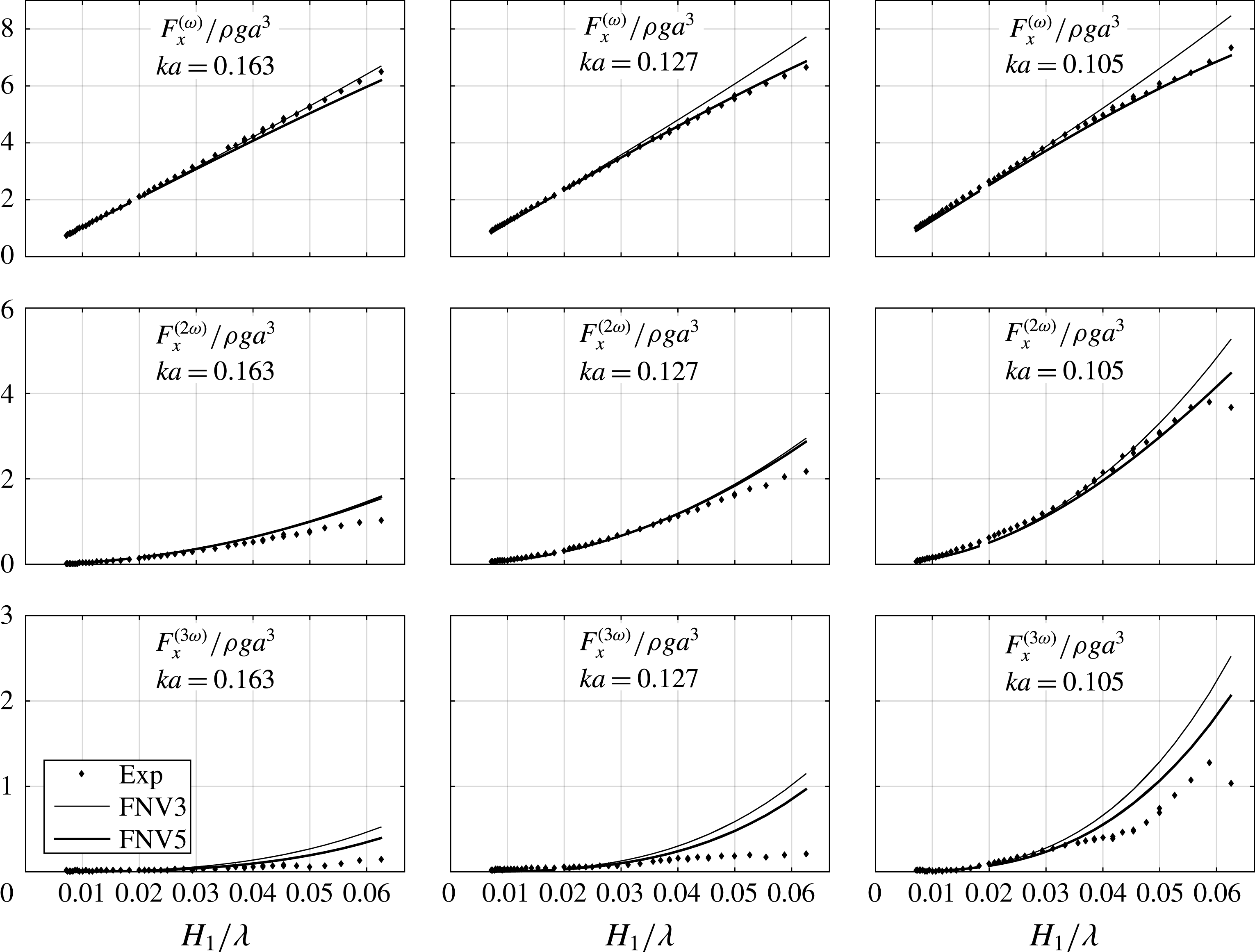
In figure 17, the amplitudes of the first three harmonics for three selected values of
 $ka$
, corresponding to long wavelengths, are presented as a function of
 $H_{1}/\unicode[STIX]{x1D706}$
. The scale in the vertical axis is the same for each harmonic for illustrative purposes. There are two theoretical curves. The thin curve represents the method (2.7), i.e. the purely third-order method. The thick curve refers to the direct numerical integration case explained in § 2.5. We see that the latter gives better agreement in all of the harmonics. The second harmonic is predicted well for all wave steepnesses in the longest-wave case,
 $ka=0.105$
. It is also predicted rather well for the shorter-wave conditions.
In figures 23 and 24 in appendix A, corresponding results are provided for a water depth of
 $h/a=5.51$
. The general trends are similar. At this water depth, the waves with
 $H_{1}/\unicode[STIX]{x1D706}>0.052$
broke in the case of
 $ka=0.121$
, and the
 $1/16$
wave steepness broke for
 $ka=0.145$
(cf. the discussion around figure 8).
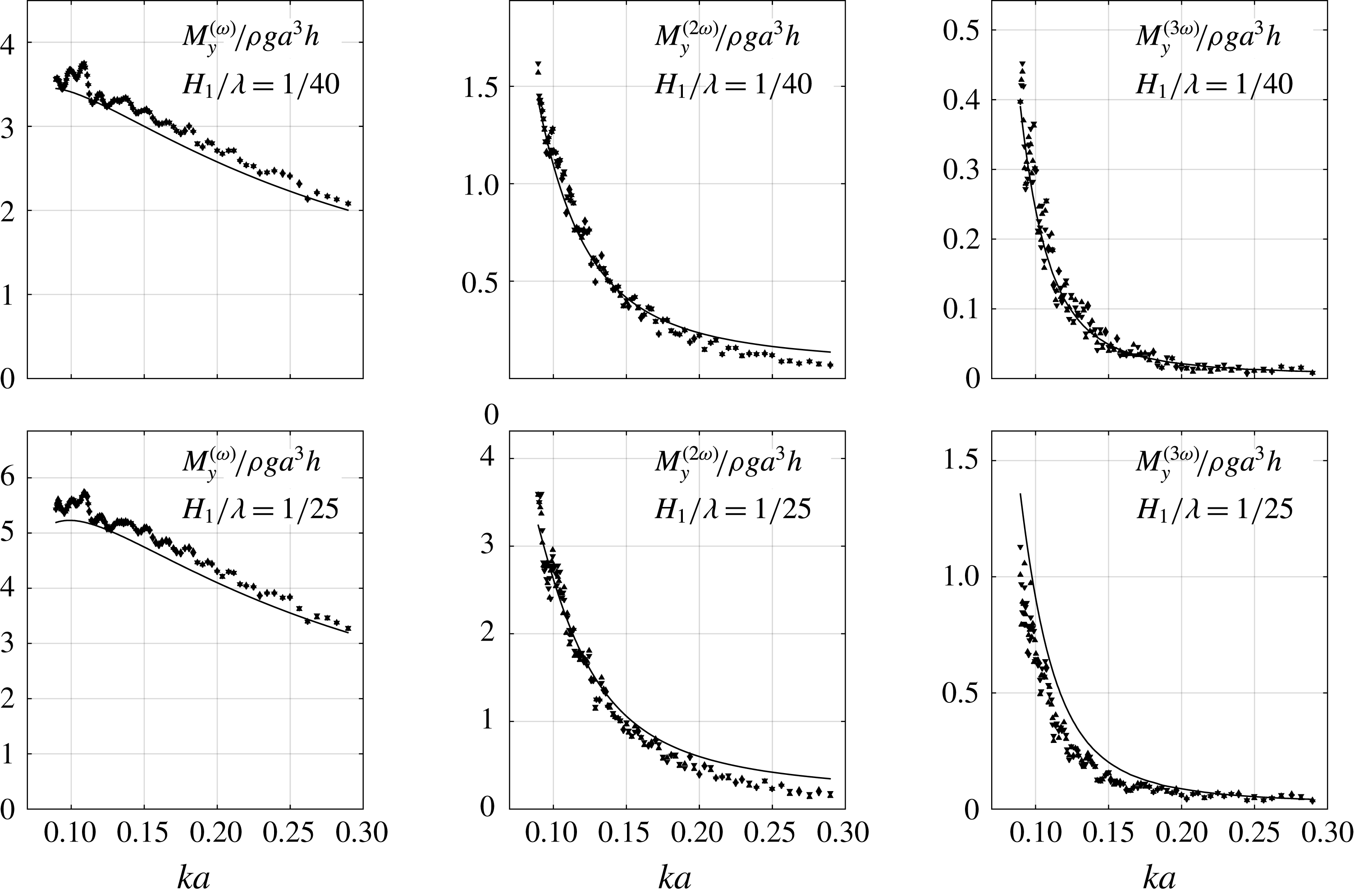
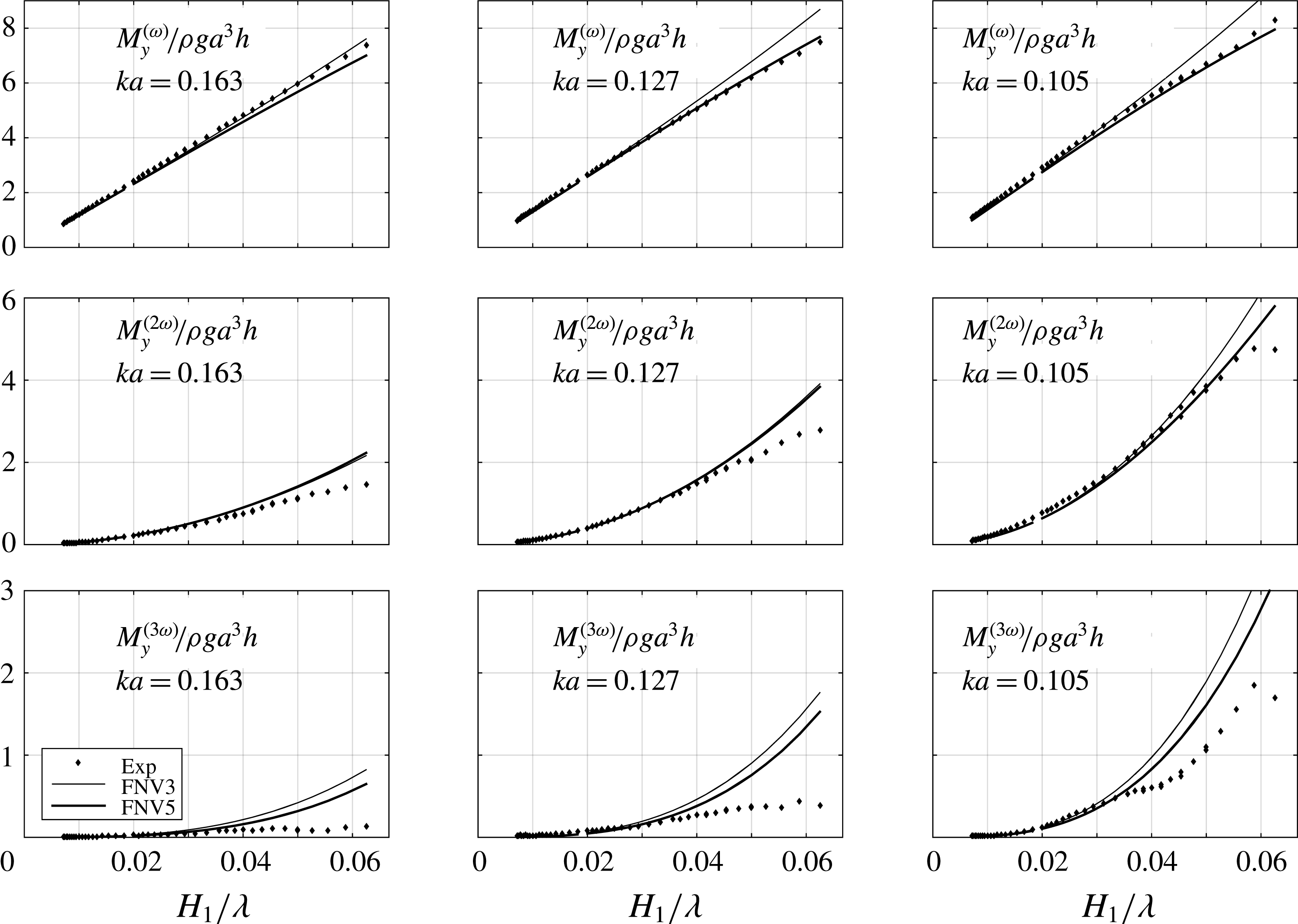
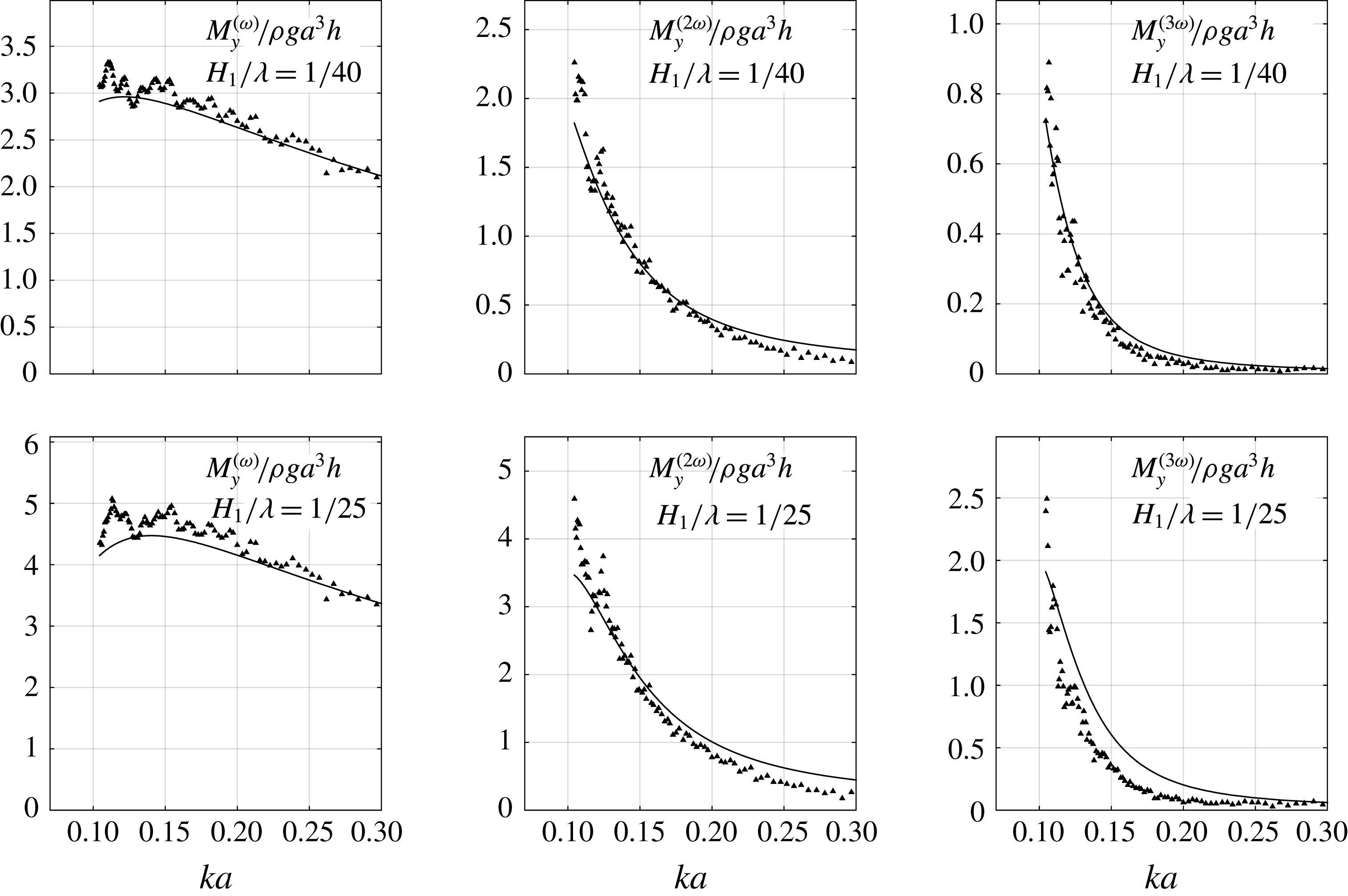
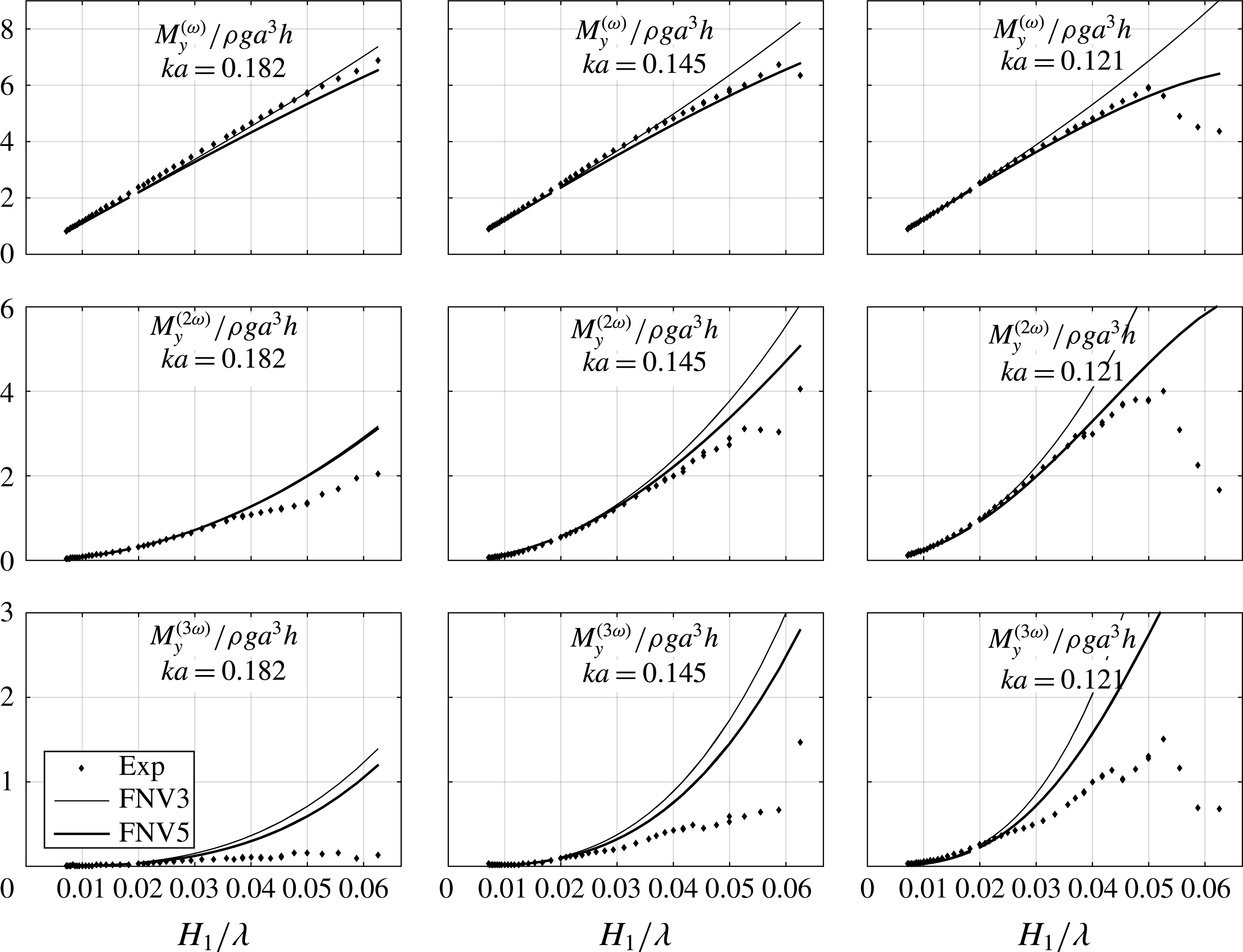
In figures 25–28 in appendix A, corresponding figures are provided for the mudline moment,
 $M_{y}$
. The trends are similar to those of the horizontal force.
The fourth and fifth harmonics of the horizontal force (a,b) and mudline moment (c,d) for two wave steepnesses
 $H_{1}/\unicode[STIX]{x1D706}=1/40$
and
 $1/25$
. The water depth is
 $h/a=7.83$
. Solid curves: generalized FNV theory. Symbols: experiments. Superscripts indicate harmonics.

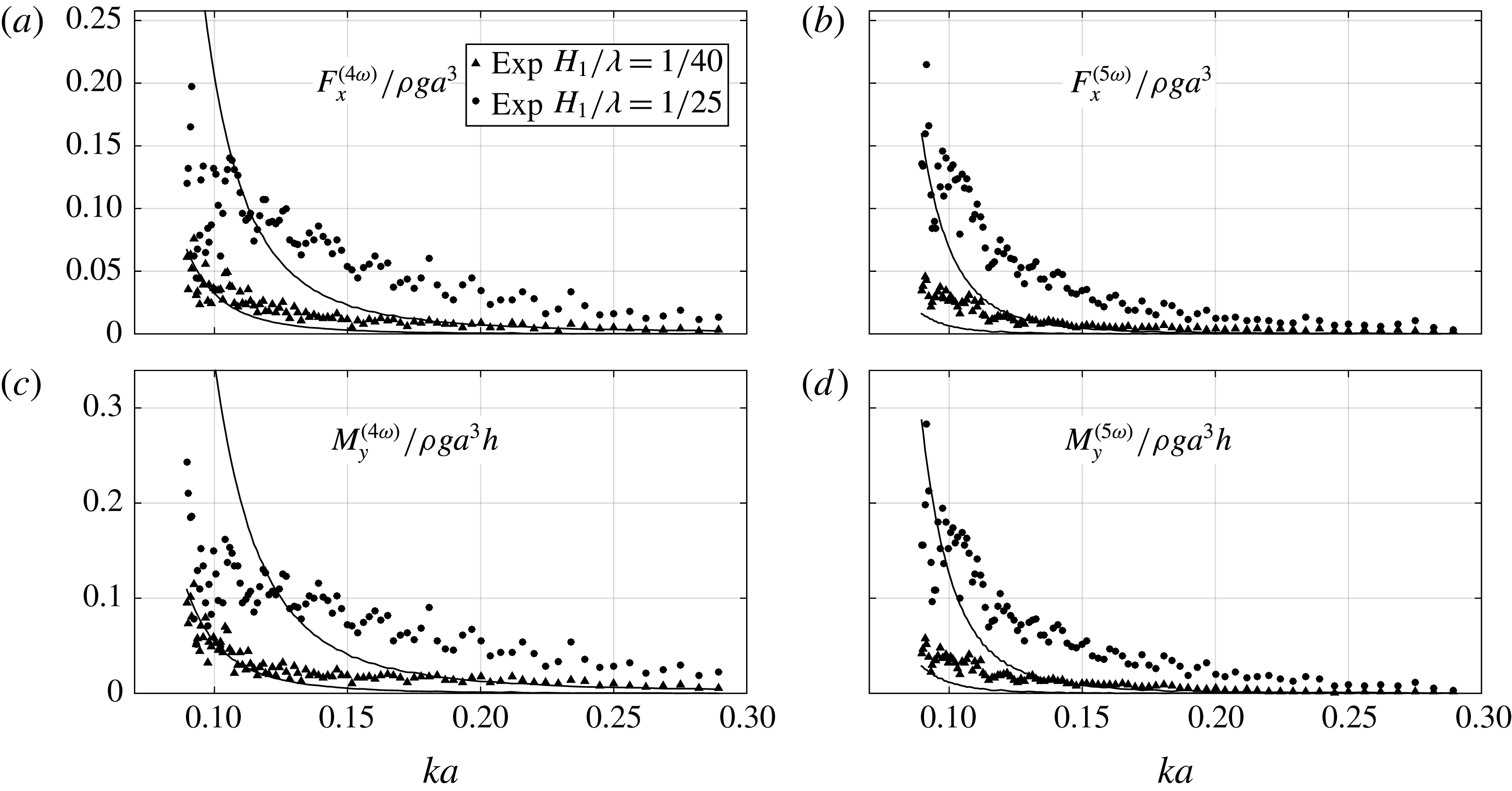
As documented in previous experiments (e.g. Huseby & Grue Reference Huseby and Grue2000), there are significant higher harmonic components also in the present experimental data. This is exemplified in figure 18, showing the fourth and fifth harmonics of the horizontal force and mudline moments as a function of
 $ka$
for two wave steepnesses. The non-dimensional values are not insignificant relative to the third harmonic components shown in the previous figures. The amplitude of the fifth harmonic is in fact higher than that of the fourth harmonic for the longest waves. The solid curves represent the approach in § 2.5, i.e. values obtained by the generalized FNV theory using Stokes fifth-order wave theory integrated to the instantaneous fifth-order free surface.
The point of attack
 $z_{p}=M_{y}/F_{x}$
of the first three harmonics. The white symbols in (a,c) represent repetition tests. FNV3: original FNV method. FNV5: applying Stokes fifth-order wave theory integrated to the instantaneous fifth-order free surface. Analytic: linear potential-flow theory using long-wavelength theory with mass coefficient
 $C_{m}=2$
.

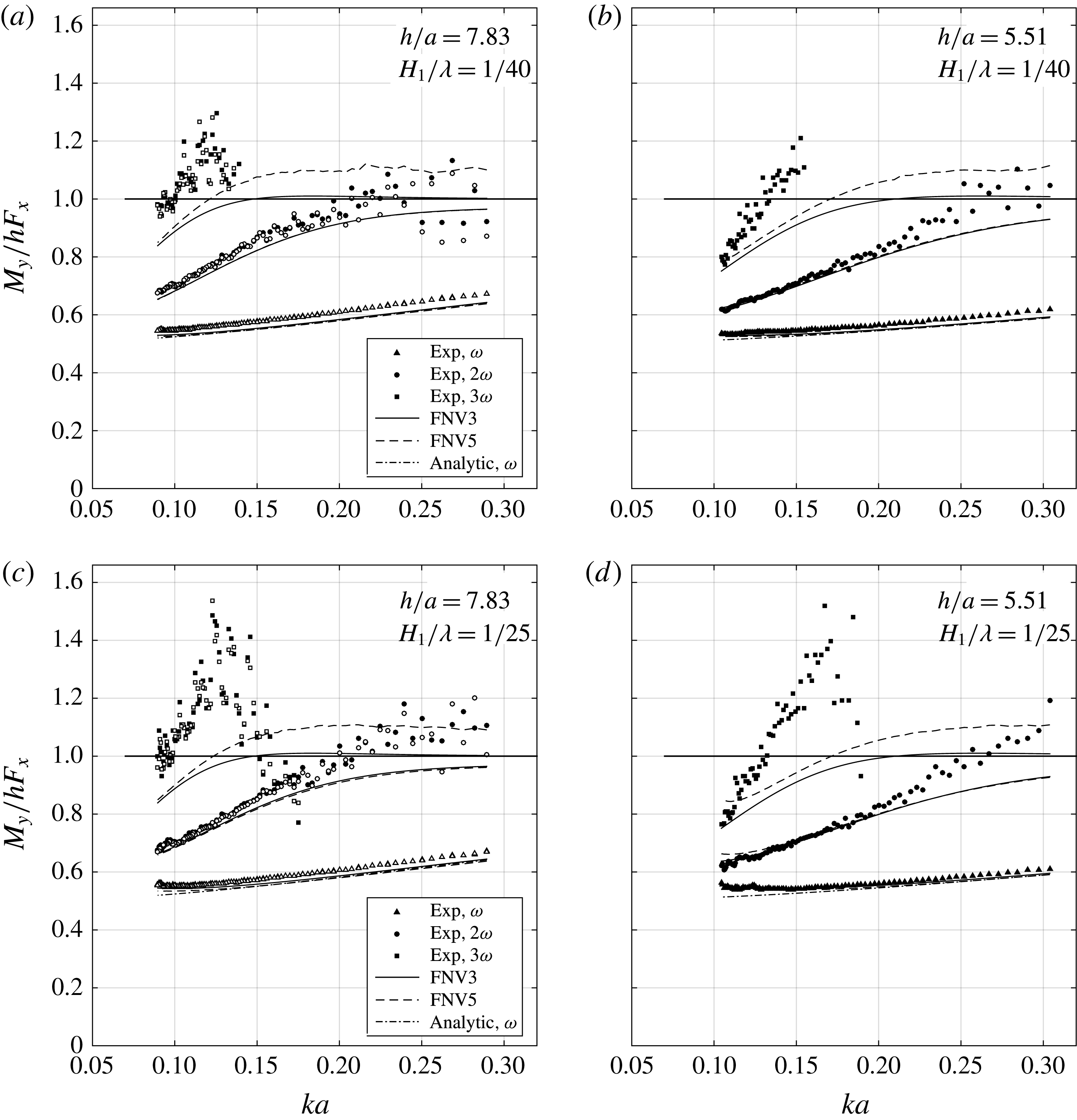
Finally, it is interesting to investigate the point of attack,
 $z_{p}=M_{y}/F_{x}$
, of the wave loads. In figure 19,
 $z_{p}$
for the first three harmonic components normalized by the water depth
 $h$
is presented for two wave steepnesses and for both of the investigated water depths. Experimental data and theoretical values using both methods described in § 2.3 and § 2.5 to calculate the generalized FNV loads are presented. The curve indicated as ‘Analytic,
 $\unicode[STIX]{x1D714}$
’ represents the first harmonic as predicted by potential-flow theory with the mass coefficient
 $C_{m}=2$
applied stripwise along the cylinder using linear wave theory. Here,
 $C_{m}=1+C_{a}$
, where
 $C_{a}=1$
represents the theoretical added mass coefficient for a circular cylinder. The analytic curve is not easy to see in all of the figures, due to the fact that it is very close to that predicted by the FNV theory.
For the first harmonic, despite small systematic differences, the experiments and theory are in good agreement. The same comment applies for the second harmonic for long waves, while for shorter waves, say
 $ka\gtrsim 0.2$
, the theory seems to, in general, underpredict
 $z_{p}$
. There is some scatter in the data for short waves. For the third harmonic, data for the short waves are removed, since they are dominated by scatter. The measured values were very small. The FNV theory with fifth-order Stokes wave theory, referred to as FNV5 in the figure, predicts that
 $z_{p}>0$
for a range of wavenumbers. The presented data also show this, and they do indeed indicate an approach towards the theoretical value, in that
 $z_{p}$
is notably higher for
 $H_{1}/\unicode[STIX]{x1D706}=1/25$
than for
 $1/40$
.
4.3 Discrepancies in the third harmonic loads
In the remaining part of the paper we focus on the discrepancies in the third harmonic of the loads.
We first investigated the importance of viscous flow separation by a strip theory approach, using experimental
 $KC$
-dependent mass and drag coefficients obtained from published U-tube experiments (Sarpkaya Reference Sarpkaya1986; Sortland Reference Sortland1986) in a similar way to what one would do in using Morison’s equation, except that all terms in the FNV method were kept. Since the mass and drag coefficients are Reynolds-number-dependent, average values were used. The procedure was to rewrite the added mass
 $a_{11}$
as
 $(C_{m}-1)\unicode[STIX]{x1D70C}\unicode[STIX]{x03C0}a^{2}$
and add the term
 $0.5\unicode[STIX]{x1D70C}C_{D}Du|u|$
, where the mass and drag coefficients
 $C_{m}$
and
 $C_{D}$
depend on the local
 $z$
-dependent
 $KC$
number along the cylinder. Both
 $KC_{1}$
and
 $KC_{5}$
were applied. U-tube experiments are based on mono-harmonic ambient flow. The fact that the ambient cross-flow has more than one harmonic is not accounted for. The results indicated a reduction in all harmonics of the loads due to the reduction in the mass coefficient for
 $KC$
numbers larger than approximately 6. For
 $KC\leqslant 5{-}6$
, the experimental value for
 $C_{m}$
is close to the theoretical potential-flow value of 2. The first and third harmonic loads were affected by the drag load for
 $KC\gtrsim 10$
, corresponding only to the most severe waves. However, neither effect was able to explain the discrepancies in the third harmonic, nor did it provide any improvement in any general trends of the other harmonics; rather the opposite. Specifically, it is clear that significant discrepancies are observed for
 $KC$
numbers less than 6; there are effects at least for
 $KC=3.5{-}4$
and above.
Flow separation is expected to occur for a circular cylinder in infinite fluid in 2D sinusoidally oscillating flow at
 $KC$
numbers higher than approximately 1.2. At
 $KC$
numbers above 4–5, there will be clear vortical structures. The previous corrections with empirical
 $C_{m}$
and
 $C_{D}$
coefficients do not account for the fact that the shed vorticity and associated pressure field will influence the free-surface elevation. Furthermore, one should have in mind that the empirical
 $C_{m}$
and
 $C_{D}$
coefficients assume that Morison’s equation is correct.
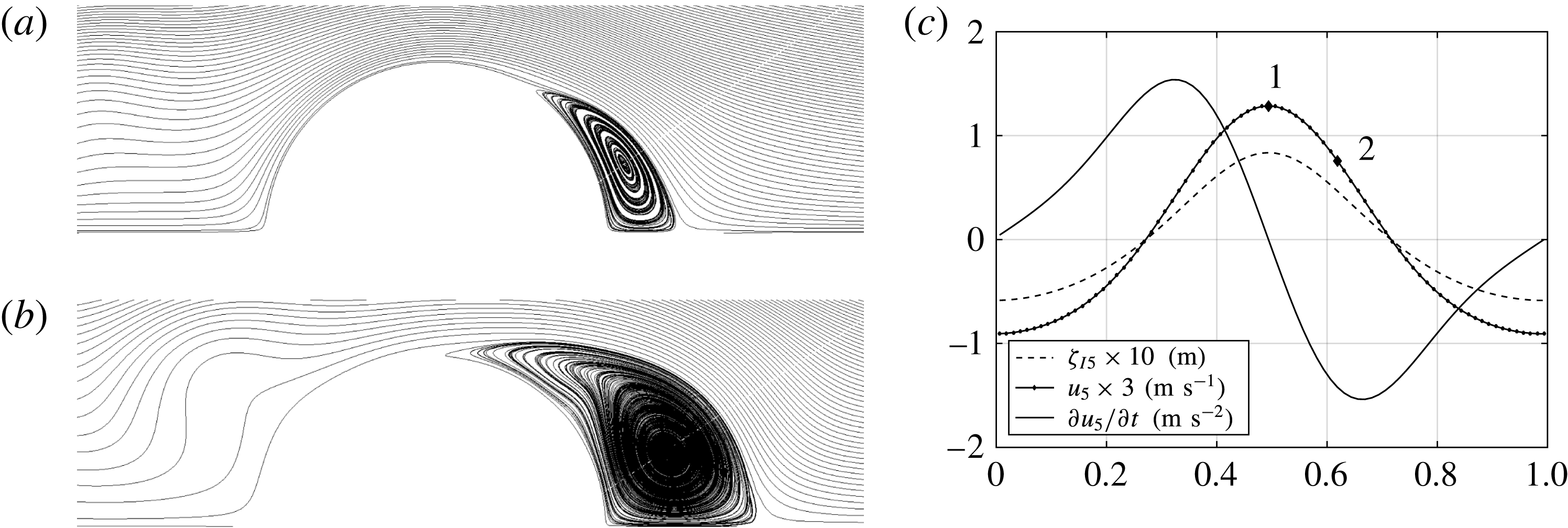
(a,b) Examples of streamlines from the present CFD simulations of flow around a circular cylinder by a Navier–Stokes large-eddy simulation (LES) solver with the cross-flow principle (M. P. Abrahamsen, personal communication, 2016). Oscillatory non-sinusoidal flow, taken as the horizontal water velocity at the free surface at the cylinder axis as calculated by fifth-order Stokes wave theory, with parameters
 $H_{1}/\unicode[STIX]{x1D706}=1/25$
, wavenumber
 $ka=0.127$
and water depth
 $h/a=7.83$
, denoted by
 $u_{5}$
in the time series. (a) Time instant 1 in the time series in (c); (b) time instant 2,
 $T/8$
later. (c) Time series of the wave kinematics;
 $\unicode[STIX]{x1D701}_{I5}$
represents the incident wave elevation at the cylinder axis, and
 $u_{5}$
and
 $\unicode[STIX]{x2202}u_{5}/\unicode[STIX]{x2202}t$
represent the horizontal water velocity and acceleration at the incident free surface at the cylinder axis respectively.

4.3.1 Simplified run-up model
To investigate the effect on the free surface due to flow separation, a simplified method is proposed. The full three-dimensional problem with a free surface is not considered. Instead, a two-dimensional Navier–Stokes solution (computational fluid dynamics; CFD) in a representative horizontal plane around the cylinder is coupled with the vertical component of the Navier–Stokes equation, which yields a prediction of the free-surface elevation close to the cylinder.
The total free-surface elevation at the cylinder wall is denoted as
 $\unicode[STIX]{x1D701}_{I5}+\unicode[STIX]{x1D701}$
, where
 $\unicode[STIX]{x1D701}_{I5}$
is the incident free surface as predicted by fifth-order Stokes theory and
 $\unicode[STIX]{x1D701}$
represents the disturbed free surface. Here,
 $\unicode[STIX]{x1D701}$
is estimated in the following manner. The vertical component of the Navier–Stokes equations is, upon neglecting the advective acceleration, viscous and turbulent stress terms,
 $$\begin{eqnarray}\unicode[STIX]{x1D70C}\frac{\unicode[STIX]{x2202}w}{\unicode[STIX]{x2202}t}=-\frac{\unicode[STIX]{x2202}p}{\unicode[STIX]{x2202}z}-\unicode[STIX]{x1D70C}g,\end{eqnarray}$$
where
 $w$
is the vertical incident wave velocity at
 $x=0$
,
 $p$
is the pressure and
 $g$
is the acceleration of gravity. We integrate the equation from
 $z=\unicode[STIX]{x1D701}_{I5}$
to
 $z=\unicode[STIX]{x1D701}_{I5}+\unicode[STIX]{x1D701}$
by assuming constant
 $\unicode[STIX]{x2202}w/\unicode[STIX]{x2202}t$
and use the fact that the pressure is zero at
 $z=\unicode[STIX]{x1D701}_{I5}+\unicode[STIX]{x1D701}$
, and equal to the pressure calculated by the CFD,
 $p_{C}$
, at
 $z=\unicode[STIX]{x1D701}_{I5}$
. The result is
 $$\begin{eqnarray}p_{C}=\unicode[STIX]{x1D70C}\left(g+\frac{\unicode[STIX]{x2202}w}{\unicode[STIX]{x2202}t}\right)\unicode[STIX]{x1D701}.\end{eqnarray}$$
In reality, the flow is three-dimensional. The reasoning behind applying two-dimensional CFD is based on assuming that the cross-flow principle is valid. This means that we neglect the effect on the flow due to the vertical water motions. This is generally found to be valid in studies of cylinders in infinite fluid, when the angle between the flow and the cylinder axis is
 $45^{\circ }{-}60^{\circ }$
or less. The kinematics in the chosen incident wave obeys the latter fact, in particular since the horizontal excursions of the water particles are considerably larger than the vertical ones in the presently considered finite water depth.
Details of the CFD simulation are described in appendix B. Examples of streamlines are provided at two time instants in figure 20(a,b). There are clear vortical structures forming downstream of the cylinder.
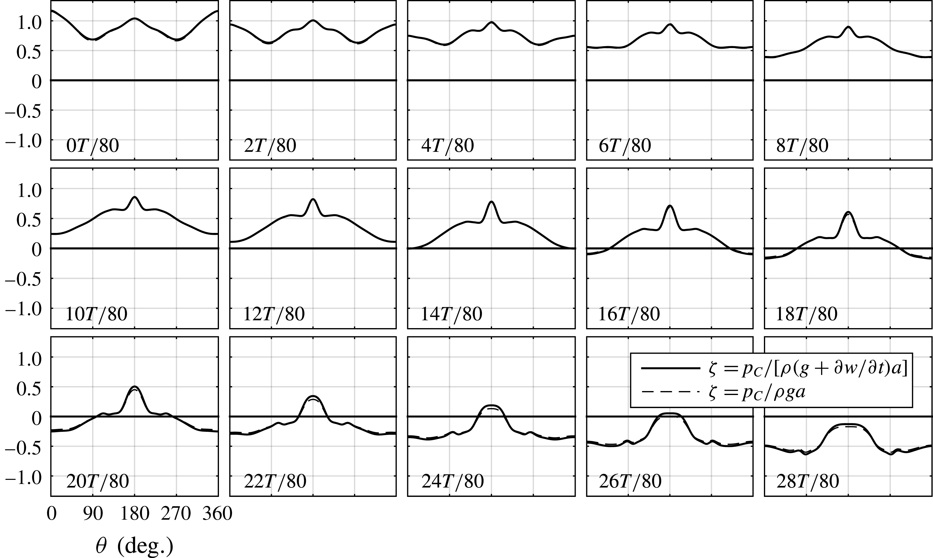
Free-surface elevation
 $\unicode[STIX]{x1D701}_{I5}+\unicode[STIX]{x1D701}$
along the cylinder wall as predicted by the simplified model (4.2) at selected time instants,
 $T/80$
apart. Here,
 $\unicode[STIX]{x1D701}_{I5}$
is the total incident free surface predicted by fifth-order Stokes wave theory, while
 $\unicode[STIX]{x1D701}$
is the diffracted free surface. The first instant corresponds to the incoming undisturbed wave crest being at the cylinder axis. The steep local run-up that forms at the rear of the cylinder (
 $180^{\circ }$
) is clearly predicted by the CFD, as well as its spreading out.

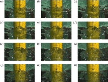
The same wave conditions as in figure 5, but rear view. Illustration of the local run-up at the rear. The time instants are approximately
 $T/40$
apart, where
 $T$
is the wave period.

In figure 21, the instantaneous value of the wave elevation at the cylinder wall,
 $\unicode[STIX]{x1D701}$
, normalized by the cylinder radius
 $a$
, as predicted by the simplified model (4.2), is provided for selected time instants. The term
 $\unicode[STIX]{x2202}w/\unicode[STIX]{x2202}t$
has a small influence on
 $\unicode[STIX]{x1D701}$
, meaning that the ‘hydrostatic’ term
 $p_{C}/\unicode[STIX]{x1D70C}g$
is sufficient for the present purpose. A local rear run-up is clearly predicted. This is not present if we use the pressure predicted by the FNV theory. The run-up is at first narrow and increasing in height. As time proceeds, the run-up widens as its height decreases. Snapshots from video were provided in figure 5, and additional snapshots, directly from the rear, are provided in figure 22; cf. also the supplementary movie. The predicted run-up amplitude is approximately 25 % lower than that observed by the video. It appears that the run-up starts to widen at an earlier stage in the experiment than that predicted. One reason may be that it becomes so steep that it breaks laterally in the experiments. In our simplified model (4.2), only the linear acceleration term is included, while the nonlinear terms are needed to predict wave breaking. Another clear simplification of our model is that the simulations are 2D, with a cross-flow principle assumption. In reality, the flow is 3D. This might influence the flow separation, but the possible significance is not known from the present study. Furthermore, there is an interaction between the free surface and the flow below, which is not accounted for. In particular, the free-surface elevation might influence the flow separation.
An estimation of the load due to the local run-up was attempted by integrating
 $p_{C}$
around the cylinder. This provides a 2D load history containing several harmonics. It is interesting to note that the predicted third, fourth and fifth harmonics are of the same order, as observed in the experiments; compare figures 15 and 18. In order to explain the discrepancy of
 $F_{x}^{(3\unicode[STIX]{x1D714})}/\unicode[STIX]{x1D70C}ga^{3}\simeq 0.13$
for this wave condition, the predicted force due to
 $p_{C}$
would need to extend over a depth of approximately
 $0.8h$
. This is not unrealistic, considering that the trough to crest distance is almost
 $2a$
, and that the
 $KC$
numbers are significant over a major part of the cylinder, indicating that significant flow separation can occur over a large range of the cylinder in the half-period covering the wave crest; cf. figures 3(a) and 6(a);
 $KC_{5}=5.2$
and
 $KC_{5}^{-}=3.5$
for this wave condition.
4.3.2 Other observations
The local wave propagating upstream along the circumference of the cylinder was discussed also in Paulsen et al. (Reference Paulsen, Bredmose, Bingham and Jacobsen2014), where three-dimensional CFD simulations with a free surface were performed for similar wave conditions and water depth to those in the present work. In the steepest wave condition, the local run-up becomes so locally steep that it breaks laterally, as observed in our experiments. The local upstream wave propagation along the circumference of the cylinder was discussed.
The local rear run-up is not restricted to the immediate vicinity of the cylinder wall only; the run-up extends downstream by a length of the order of the cylinder diameter. This is clearly observed in the present experiments as well as the simulations by Paulsen et al. (Reference Paulsen, Bredmose, Bingham and Jacobsen2014), and was described earlier by Chaplin et al. (Reference Chaplin, Rainey and Yemm1997). In Chaplin et al. (Reference Chaplin, Rainey and Yemm1997), this phenomenon is referred to as a ‘mound’, something we find to be a descriptive phrase. Another descriptive phrase may by ‘upwelling’.
During the present experiments, we attempted to visually observe the flow at the free surface using confetti (remnants are seen in figures 5 and 22). Rather than observing vortical structures forming on the free surface, the confetti was displaced away from the area occupied by the mound during each wave period, and it did not return. It was clear that an upwelling from below was taking place. This is consistent with the idea that a high pressure formed beneath the free surface due to flow separation is causing the upwelling, seen as local run-up on the cylinder wall.
Since the incident horizontal velocity at the free surface at the cylinder axis is, for instance, clearly different if there is an incident wave crest or a wave trough (cf. figure 3), the flow separation is not the same in the half-period starting with an incident wave node at the cylinder axis, including the incident wave crest at the cylinder axis, as it is for the other half-period, including the incident wave trough at the cylinder axis. This is consistent with the fact that the local run-up is observed only at the rear, and not in the front of the cylinder in the experiments.
The discussion above provides consistent evidence that the mound with local rear run-up is caused by a high-pressure zone which is formed due to flow separation.
4.4 Comments
Several authors have discussed the so-called ‘secondary load cycle’ rather extensively. The secondary load cycle is a distinct short-duration load time history with a peak just after the main load peak. It was observed and described in terms of force time series from experiments with focused wave groups, and termed secondary oscillation in Grue et al. (Reference Grue, Bjorshol and Strand1994). Later, it was named the secondary load cycle by Chaplin et al. (Reference Chaplin, Rainey and Yemm1997), where also snapshots showing the rear mound were provided from tests in a glass wall wave tank. The typical duration of the secondary load cycle is reported to be around one-sixth of the underlying wave period. Typical wave conditions where it appears are discussed, for instance, by Huseby & Grue (Reference Huseby and Grue2000) in the initial transient phase of regular wave trains and in large irregular wave events. They investigated deep water wave conditions. More recently, Paulsen et al. (Reference Paulsen, Bredmose, Bingham and Jacobsen2014) discussed this in their study using a fully nonlinear numerical wave tank, with similar regular wave conditions to the present selected cases. Their CFD computations predicted the short-duration load with a peak. They had a higher wave steepness than our selected case. They investigated the phenomenon by using a single-vortex method. In all of the abovementioned papers, the secondary load cycle is associated with a short-duration peak after the main force peak in the force time series. In our case (figure 14), the short-duration load with a peak does not appear. Still, although a distinct peak in the load time series does not appear, it is appropriate to denote by the local run-up phenomenon the term secondary load cycle, since it seems to give rise to a range of load harmonics (reducing the third harmonic, but introducing significant fourth and fifth harmonics).
The FNV theory is a perturbation theory. The present study indicates that it is indeed correct for the third harmonic up to some limiting wave steepness, depending on the water depth and its theoretical assumption about no far-field wave generation by the cylinder, and that flow separation is insignificant. In the present conditions,
 $H_{1}/\unicode[STIX]{x1D706}=1/40$
seems to be a reasonable limit. Above this limit, it is argued that viscous flow separation causes significant discrepancies. In severe irregular wave events, the local steepness is typically significantly higher than this. It remains to be investigated whether the discrepancies are equally pronounced in an irregular sea state. We leave it as a challenge to develop a rational load model that is able to quantitatively describe the discrepancies. At present, only 3D CFD is able to capture this, but the use of CFD is not practical in design due to the time consumption associated with running a large number of three hour duration sea states. Computational fluid dynamics may well be used in the development of rational load models, in combination with theory and experiments.
5 Conclusions
The FNV method for calculation of higher-order wave loads on a vertical circular free-surface-piercing bottom-mounted non-moving cylinder was generalized to finite water depth. The method is based on potential flow of an incompressible fluid, with its theoretical assumption that there is no far-field wave generation by the cylinder and that flow separation is insignificant. Systematic regular wave experiments were carried out, mostly in intermediate depth wave conditions, and the harmonics of the horizontal loads were compared with the generalized FNV theory. Significant effects of flow separation were shown to be present in medium to steep wave conditions.
Load measurements included the horizontal force and the mudline overturning moment. Several measures were taken to establish confidence in the quality of the data. Two different load measurement set-ups were used. The purpose was to check whether the first force and moment transducer set-up was adequately accurate. The results were basically identical. Parasitic waves were reduced by adding a
 $2\unicode[STIX]{x1D714}$
signal to the wave maker. Here,
 $\unicode[STIX]{x1D714}$
is the basic frequency of the regular wave. Repetition tests were performed. Wave reflections from a parabolic shaped beach were investigated. Different time windows were used for extraction of the reduced data. An automatic test procedure was used, enabling systematic tests. Although there were variations in individual tests, the main trends were not affected by the different actions.
Load terms oscillating with
 $\unicode[STIX]{x1D714}$
,
 $2\unicode[STIX]{x1D714}$
,
 $3\unicode[STIX]{x1D714}$
,
 $4\unicode[STIX]{x1D714}$
and
 $5\unicode[STIX]{x1D714}$
were studied. The main focus was on the loads oscillating with
 $3\unicode[STIX]{x1D714}$
. The theoretically predicted third harmonic loads were shown to agree well with the experiments for small to medium wave steepness, up to a rather distinct limiting wave steepness. Above this limit, the theory overpredicted, and the discrepancy in general increased monotonically with increasing wave steepness. The local
 $KC$
number along the axis of the cylinder indicated that flow separation occurred for the wave conditions where there were discrepancies. Assuming
 $KC$
-dependent added mass coefficients, and adding a drag term in the FNV model, as is done in Morison’s equation, did not explain the discrepancies. A distinct run-up at the rear of the cylinder was observed in the experiments. A simplified numerical model assuming the cross-flow principle was proposed, based on a 2D Navier–Stokes solver combined with LES with imposed oscillatory flow representative for a chosen wave condition. Locally high pressure at the rear of the cylinder, due to flow separation leading to distinct vortical structures, was shown to cause the local run-up. The duration of the run-up was approximately one-quarter to one-third of the wave period. The run-up resulted in a local steep wave propagating against the incident wave propagation. The load associated with the run-up and subsequent steep local wave propagating is believed to be the cause of significant
 $3\unicode[STIX]{x1D714}$
,
 $4\unicode[STIX]{x1D714}$
and
 $5\unicode[STIX]{x1D714}$
loads.
Acknowledgements
The authors acknowledge Statoil for allowing the use of the experimental set-up used by SINTEF Ocean (former MARINTEK) in qualifying the Dudgeon offshore wind farm. The work carried out by F. Bickert performing tests in the laboratory during his internship at NTNU is acknowledged. The authors acknowledge the financial support of the Centre of Autonomous Marine Operations and Systems (AMOS), whose main sponsor is the Norwegian Research Council (Project no. 223254-AMOS).
Supplementary movie
A supplementary movie is available at https://doi.org/10.1017/jfm.2017.702.
Appendix A. Load harmonics
The first three harmonics of the measured forces and moments are given as a function of the wavenumber
 $ka$
in figures 23, 25 and 27, and as a function of the wave steepness
 $H_{1}/\unicode[STIX]{x1D706}$
in figures 24, 26 and 28.
Amplitudes of the first three harmonics of the horizontal force due to regular waves at water depth
 $h/a=5.51$
. Superscripts indicate harmonics.

Amplitudes of the first three harmonics of the horizontal force due to regular waves at water depth
 $h/a=5.51$
. Superscripts indicate harmonics.

Amplitudes of the first three harmonics of the mudline moment due to regular waves at water depth
 $h/a=7.83$
. Superscripts indicate harmonics.

Amplitudes of the first three harmonics of the mudline moment due to regular waves at water depth
 $h/a=7.83$
. Superscripts indicate harmonics.

Amplitudes of the first three harmonics of the mudline moment due to regular waves at water depth
 $h/a=5.51$
. Superscripts indicate harmonics.

Amplitudes of the first three harmonics of the mudline moment due to regular waves at water depth
 $h/a=5.51$
. Superscripts indicate harmonics.

Appendix B. Main parameters in the LES simulation
The CFD simulations were carried out by an LES solver based on the finite volume method with model scale measures corresponding to the experiments, using OpenFOAM. The forced flow was taken as a representative flow for one of the conditions where significant discrepancies in the third harmonic loads were observed:
 $ka=0.127$
with
 $H_{1}/\unicode[STIX]{x1D706}=1/25$
at
 $h/a=7.83$
. The water particle velocities at the incident wave crest, as predicted by fifth-order Stokes wave theory, were used as boundary conditions in the simulation.
The prescribed flow was 2D, while, due to the fact that LES is intrinsically a 3D simulation technique, the actual LES computations were carried out in 3D with a cylinder length
 $l=3a$
in uniform oscillating flow. The cylinder was discretized by 10 equidistant cells along its axis. There were only very small variations of the simulated flow along the cylinder. The presented results are taken at one of the two middle cross-sections. The extent of the computational domain was
 $(x/a,y/a)=(\{-26.4,26.4\},\{-20.9,20.9\})$
. The ambient oscillatory flow was in the
 $x$
-direction. The total number of cells was 929.300, meaning 92.930 in each cross-section. In the vicinity of the cylinder, the mesh was discretized by 480 equidistant cells along its perimeter. The radial resolution was finest at the cylinder wall, with
 $\unicode[STIX]{x0394}r/a=0.0031$
, smoothly increasing away from the cylinder.
We do not know whether the boundary layers will be laminar or turbulent in the present conditions. Flow separation is, however, likely to occur in both cases, causing the same physical effect of a local rear run-up. A dedicated future study would be needed to quantitatively asses the effect of turbulence in the boundary layer flow. In the cases where the boundary layer flow was laminar, the number of cells over the boundary layer was approximately 10, using the measure
 $\unicode[STIX]{x1D6FF}_{0.99}=4.6\sqrt{2\unicode[STIX]{x1D708}/\unicode[STIX]{x1D714}}$
for the boundary layer thickness, which is the distance from the wall where the velocity attains 99 % of the local velocity outside the boundary layer in sinusoidally oscillating flow with frequency
 $\unicode[STIX]{x1D714}$
. The time step was
 $\unicode[STIX]{x0394}t/T=2.9\times 10^{-4}$
.
The duration of the simulation was eight oscillation periods. The second last period is used in this study. On 32 cores, the simulation time, running eight oscillations, was approximately 13 h.