



1. Introduction
Turbulent flows exert unsteady wall pressure loadings over solid walls. The wall pressure fluctuations (WPF) play an essential role in sonic loading in rocket sensor fairings, flow noise inside towed sonar arrays, and flow-induced vibration of pipelines. A clear characterisation and understanding of their statistics, spectra and control is crucial in the aviation and ocean engineering industry (Blake Reference Blake1970).
Extensive research has been conducted to characterise the WPF beneath turbulent boundary layers, with early research mainly on incompressible flows over flat plates. Willmarth (Reference Willmarth1956) appeared to be the first to measure basic statistics such as the root mean square (rms) value and frequency spectra of the WPF. Further experiments conducted by Harrison (Reference Harrison1958) and Willmarth (Reference Willmarth1958) studied the WPF space–time correlation, and showed that the convection velocity was approximately
 $80\,\%$
of the freestream velocity. Bull (Reference Bull1967), on the other hand, reported that the convection velocity depends on frequency. Regarding analytical models, Kraichnan (Reference Kraichnan1956) was among the first to develop a mirror-flow model, and showed that the rms value of the WPF was approximately six times the mean wall shear stress, a result that agreed well with the measured values by Willmarth (Reference Willmarth1956) and many others (Bull Reference Bull1996). Based on streamwise and lateral correlation similarity, Corcos (Reference Corcos1963) proposed a model for the cross-spectral density of the WPF, applicable to the wavenumber regime near
 $\omega /U_c$
, where
 $\omega$
and
 $U_c$
represent the angular frequency and convection velocity of the WPF, respectively. Comprehensive reviews of these early studies can be found in Willmarth (Reference Willmarth1975) and Bull (Reference Bull1996).
However, realistic applications often involve wall surfaces with curvature, such as the hose of a towed sonar array. Incompressible WPF over curved surfaces were studied subsequently. This includes, for example, early experiments by Willmarth & Yang (Reference Willmarth and Yang1970) and Willmarth et al. (Reference Willmarth, Winkel, Sharma and Bogar1976). They concluded that the wall curvature caused insignificant changes in the frequency spectra and convection velocity, but a noticeable reduction in the spanwise correlation length. Analytical modelling was conducted by Howe (Reference Howe1987) and Dowling (Reference Dowling1998), the latter of which modelled the incompressible wavenumber–frequency spectrum using the Lighthill acoustic analogy. The effect of wall curvature on WPF was also examined using direct numerical simulations (DNS), where Neves & Moin (Reference Neves and Moin1994b ) showed that increasing curvature reduced both spatial and temporal spectra of the WPF at all scales, decreased the azimuthal correlation length, increased the streamwise correlation length, and reduced the convection velocity. Note that the curvature examined in their studies was substantially larger than that in Willmarth & Yang (Reference Willmarth and Yang1970) and Willmarth et al. (Reference Willmarth, Winkel, Sharma and Bogar1976).
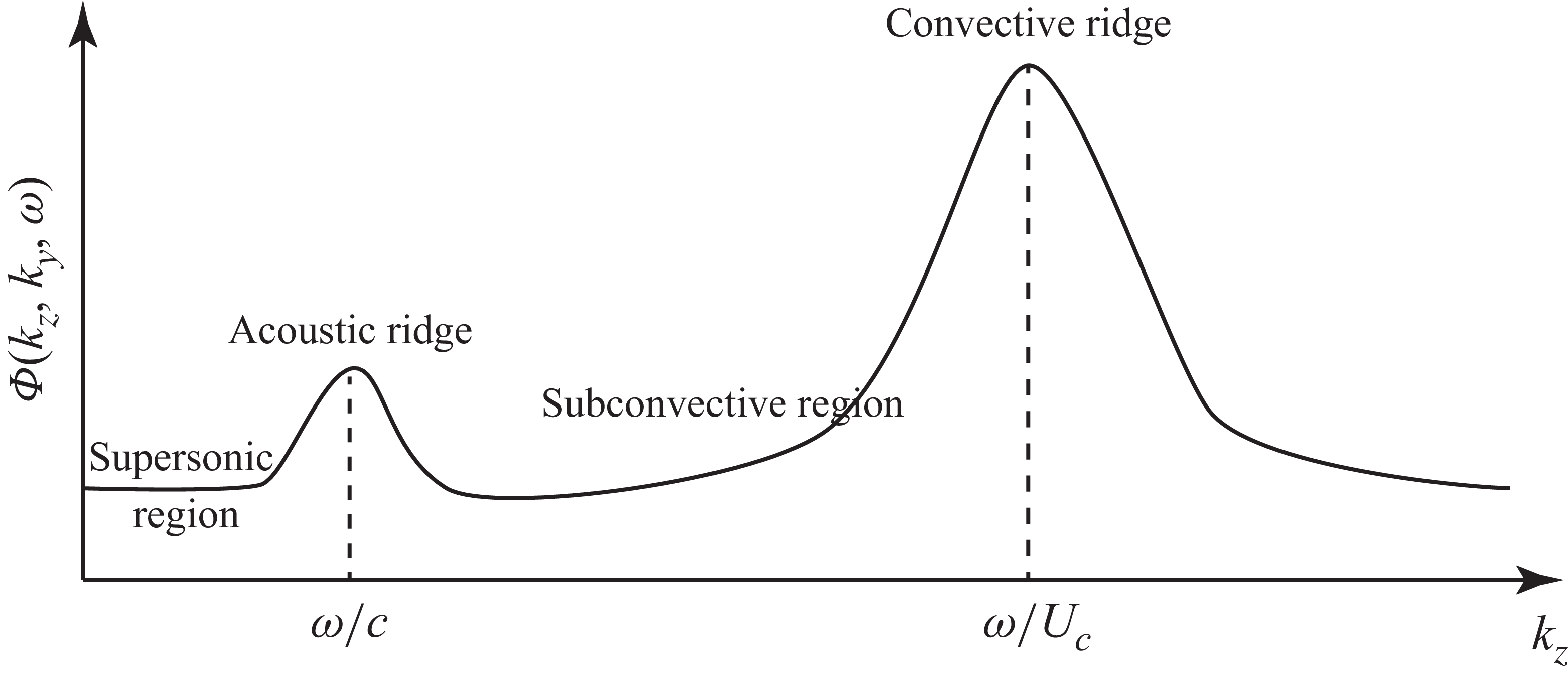
A typical wavenumber–frequency spectrum at a given angular frequency
 $\omega$
is shown in figure 1. A high-wavenumber peak called the convective ridge is located at
 $k_z = \omega / U_c$
due to turbulence convection, where
 $k_z$
represents the streamwise wavenumber. In contrast, a low-wavenumber acoustic ridge appears at
 $k_z = \omega / c$
, where
 $c$
is the speed of sound. Note, however, that it is the low-wavenumber components of the WPF, i.e. the subconvective and supersonic regions shown in figure 1, that are of particular interest in practice. This is because they are more likely to couple with the elastic motion of the solid walls, or are responsible for direct acoustic radiation. In such regimes, compressibility is crucial, even in very low Mach number flows; it is therefore essential to include the effects of compressibility in the study of WPF. For example, using the Lighthill acoustic analogy, Ffowcs-Williams (Reference Ffowcs-Williams1965) showed that including compressibility resulted in the violation of the Kraichnan–Phillips theorem, and led to a non-zero spectral magnitude proportional to the square of the mean-flow Mach number at zero wavenumbers.
A typical wavenumber–frequency spectrum of the WPF at a given frequency
 $\omega$
and spanwise wavenumber
 $k_y=0$
. Here,
 $k_z$
represents the streamwise wavenumber.

The magnitude of the wavenumber–frequency spectrum around the acoustic ridge, as can be seen from figure 1, is often much lower than that near the convective ridge. This poses significant challenges to resolving the low-wavenumber components using either experiments or numerical simulations. As such, compressible simulations that study the subconvective and supersonic regions remain scarce. Gloerfelt & Berland (Reference Gloerfelt and Berland2013) and Cohen & Gloerfelt (Reference Cohen and Gloerfelt2018) were among the first to study the acoustic component of the WPF beneath a turbulent boundary layer at Mach 0.5 using large-eddy simulations. They were able to capture the acoustic ridge, but were unable to fully eliminate errors caused by artificial boundaries. A recent study by Liu, Wang & Wang (Reference Liu, Wang and Wang2024) showed that with suitable choices of low-dissipative and low-dispersive schemes, it is possible to accurately resolve these low-energy components using compressible DNS. The DNS were performed on a rectangular channel with periodic boundary conditions to suppress the artefacts introduced by the boundary conditions.
However, as mentioned above, practical applications are characterised rarely by flat plates, but rather by surfaces with curvature. To the best of the authors’ knowledge, compressible flow simulations focusing on the low-wavenumber region of the WPF over surfaces with curvature remain to be seen. The characteristics of the low-wavenumber components of the WPF over cylindrical walls – in particular, how energetic they are compared to convective components as the curvature varies – remain largely unknown. In this paper, we aim to bridge the gap and study the wall pressure over cylindrical surfaces of various curvatures. To directly resolve these low-wavenumber components, we resort to DNS with low-dissipative and low-dispersive finite-difference schemes. Similar to Liu et al. (Reference Liu, Wang and Wang2024), to avoid the inevitable noise introduced by artificial boundary conditions, channel flows within a concentric annular duct are simulated with a periodic boundary condition in the streamwise direction. In doing so, not all the features of the free boundary layer can be captured, but the important effects of curvature are kept without complications introduced by simulating free boundary layers (Neves & Moin Reference Neves and Moin1994b ).
This paper is structured as follows. Section 2 introduces the computational set-up and discretisation schemes used in this study. Section 3 validates the simulations, and discusses the effects of curvature on flow statistics. Section 4 shows the power spectral density (PSD) and wavenumber–frequency spectra of the WPF over cylinders of various diameters. Section 5 uses the Lighthill acoustic analogy to model the WPF generated by cylindrical boundary layers, with which the mechanisms of the low-wavenumber WPF augmentation are discussed. The final section concludes the paper and lists future work.
2. Numerical set-up
A schematic set-up of the simulations is shown in figure 2. The channel flow within the annular duct is discretised on a generalised curvilinear coordinate system, with
 $\theta$
,
 $r$
and
 $z$
denoting the azimuthal, radial and axial directions, respectively. The annular duct has height
 $L_r=2\delta$
and length
 $L_z=16\pi \delta$
;
 $L_\theta$
and
 $R$
are used to denote the circumference and radius of the inner cylindrical wall, respectively. In the
 $\theta$
and
 $z$
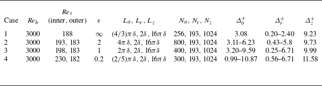
directions, grid points are uniformly distributed, with periodic conditions applied at the boundaries. A no-slip isothermal condition is imposed on the walls, and the grid near the wall is refined based on a hyperbolic tangent function. The parameters of all four DNS runs are listed in table 1, where
 $\epsilon$
is defined as
 $R/\delta$
to represent the non-dimensional radius of the inner cylinder. Case 1 is a plane channel for comparison, where
 $L_\theta$
reduces to the spanwise domain size. The spanwise domain size
 $4\pi \delta /3$
is chosen to be the same as that used by Liu et al. (Reference Liu, Wang and Wang2024) to facilitate a direct comparison and validation. Note that we have also conducted a simulation using a slightly larger spanwise domain size
 $2\pi \delta$
, resulting in little change in the spectra of the WPF. The channel length
 $L_z$
, as shown in table 1, is deliberately chosen to be
 $16\pi \delta$
in order to resolve the low-wavenumber components of the WPF.
Simulation matrix and parameters used in each simulation:
 $N_i$
and
 $\varDelta ^+_i$
represent the number and non-dimensional spacing of the grid elements in the
 $i$
direction (
 $i$
=
 $\theta$
,
 $r$
,
 $z$
).

The DNS configurations, with
 $\theta$
,
 $r$
and
 $z$
denoting the circumferential, radial and axial directions, respectively. The contours of instantaneous velocity magnitude and pressure are shown on the inlet and inner and outer walls, respectively.

The three-dimensional compressible Navier–Stokes equations are solved using the DNS method. In the Cartesian frame
 $(x_1, x_2, x_3)$
these equations can be written as
 \begin{align} \frac {\partial \rho }{\partial t} + \frac {\partial \big(\rho u_j\big)}{\partial x_{\!j}} &= 0, \\[-12pt]\nonumber \end{align}
 \begin{align} \frac {\partial \big(\rho u_i\big)}{\partial t} + \frac {\partial \big(\rho u_i u_j + p\delta _{\textit{ij}}\big)}{\partial x_{\!j}} &= \frac {\partial \tau _{\textit{ij}}}{\partial x_{\!j}}+f_3\delta _{i3}, \\[-12pt]\nonumber \end{align}
 \begin{align} \frac {\partial (\rho e_0)}{\partial t} + \frac {\partial \big[u_j\big(\rho e_0 + p\big)\big]}{\partial x_{\!j}} &= \frac {\partial \big(\tau _{\textit{ij}} u_i\big)}{\partial x_{\!j}} - \frac {\partial q_j}{\partial x_{\!j}}+f_3 u_3, \end{align}
where
 $i$
and
 $j$
take values
 $1,2,3$
, the Einstein summation notation is implied,
 $t$
denotes time, while
 $\rho$
,
 $u_i$
,
 $p$
,
 $\tau _{\textit{ij}}$
,
 $e_0$
and
 $q_j$
denote the flow density, velocity (
 $i$
th component), pressure, stress tensor, total energy and heat flux (
 $j$
th component), respectively. Moreover,
 $\delta _{\textit{ij}}$
is the Kronecker tensor, and
 $f_3$
denotes a constant driving volume force in the
 $x_3$
(axial) direction. The total energy
 $e_0$
is given by
 \begin{equation} e_0 = \frac {\rho u_i u_i}{2} + \frac {R_{\textit{gas}}}{ \gamma - 1}T, \end{equation}
where
 $\gamma = 1.4$
is the specific heat ratio,
 $R_{\textit{gas}}$
is the gas constant, and
 $T$
is the temperature. Moreover, the stress tensor is written as
 \begin{equation} \tau _{\textit{ij}} = \mu \left (\frac {\partial u_i}{\partial x_{\!j}} + \frac {\partial u_j}{\partial x_i} - \frac {2}{3}\frac {\partial u_k}{\partial x_k}\delta _{\textit{ij}}\right )\!, \end{equation}
and the molecular viscosity
 $\mu$
is computed using Sutherland’s law (White Reference White1991). Similarly, the heat flux
 $q_j$
is written as
 \begin{equation} q_j = -\frac {\mu \gamma R_{\textit{gas}} }{\textit{Pr}\,(\gamma -1)}\frac {\partial T}{\partial x_{\!j}}, \end{equation}
where
 $Pr$
is the Prandtl number, taking value
 $0.72$
.
The non-dimensionalised code HiPSTAR (Sandberg et al. Reference Sandberg, Michelassi, Pichler, Chen and Johnstone2015), which has been extensively validated for acoustic simulations (Deuse & Sandberg Reference Deuse and Sandberg2020), is used for the present simulations. The non-dimensionalisation is based on
 $\delta$
,
 $U_b$
,
 $\rho _b$
and
 $T_w$
, representing the channel half-height, mean bulk velocity, mean bulk density and wall temperature, respectively. Here,
 $\mu _\infty$
and
 $c_\infty$
are used to denote the viscosity and speed of sound for the reference state, which only depend on the reference wall temperature
 $T_w$
. The resulting Reynolds number
 ${\textit{Re}}_b = (\rho _b U_b \delta )/\mu _\infty$
is fixed at
 $3000$
, while the Mach number
 $M_b = U_b / c_\infty$
is fixed at
 $0.4$
.
A fourth-order finite difference scheme was applied for spatial discretisation, while the ultra-low storage frequency optimised explicit Runge–Kutta method (Kennedy, Carpenter & Lewis Reference Kennedy, Carpenter and Lewis2000) was used for time integration. In addition, the nonlinear terms are processed with a skew-symmetric splitting method (Kennedy & Gruber Reference Kennedy and Gruber2008) to reduce aliasing, and a standard filtering scheme (Bogey & Bailly Reference Bogey and Bailly2004) is used to improve numerical stability. Simulations are conducted for approximately 48 flow-through time units on GPUs, after which the wall pressure on the inner cylinder surface and velocity data within the channel are stored for analysis. Detailed sampling frequency and sampling duration are shown in § 4.
3. Validation and flow statistics
Before examining the WPF, we first validate the present DNS by comparing the flow statistics against those in the literature. The effects of curvature on the flow statistics are shown subsequently. To facilitate an examination of the turbulent statistics distribution along the wall-normal direction, a radial distance measured from the inner cylinder wall, defined as
 $y=r - R$
, is used. This distance is often presented in wall units defined by
 $y^+=yu_\tau /\nu$
, where
 $\nu$
and
 $u_\tau$
represent the kinematic viscosity and wall friction velocity of the flow, respectively.
3.1. Validation of the DNS
To validate the present simulations, the mean and fluctuation velocities are first compared against results published previously. Note that the fluctuation velocities are defined by removing the mean values defined by the Favre average (
 $\tilde {{\cdot }}$
), i.e.
 \begin{align} \tilde {u}_i &= \langle \rho u_i \rangle / \langle \rho \rangle , \end{align}
 \begin{align} u_i^\prime &= u_i - \tilde {u}_i, \end{align}
where
 $\langle {\cdot }\rangle$
represents ensemble average. In practice, temporal and spatial (streamwise and azimuthal) averages are used instead. It is worth noting that although the bulk Mach number
 $M_b$
is
 $0.4$
, the density variation of the flow is very limited. As such, the difference between the direct and Favre averages is negligible. The mean and fluctuation velocities are subsequently normalised by the friction velocity
 $u_\tau$
to obtain
 $\tilde {u}_i^+$
and
 $u_i^{\prime +}$
, respectively.
The comparison of the two velocities is shown in figure 3, where figure 3(a) shows the distribution of the axial mean velocity along the wall-normal direction. In the rectangular case, the viscous sublayer and log law of the wall are captured and compared well with Liu et al. (Reference Liu, Wang and Wang2024). When the radius of the inner cylinder reduces to
 $\epsilon =2$
or
 $1$
, the velocity distribution shows minimal change, in contrast to the significant changes at
 $\epsilon =0.2$
. In particular, the axial mean velocity decreases in the outer layer. The obtained velocity profile agrees well with Bagheri & Wang (Reference Bagheri and Wang2020), albeit with slight mismatches in the inner cylinder radius.
Comparison of (a) mean velocity profiles and (b) rms of velocity fluctuations between the present cases and previous simulations. Circles indicate the plane-channel case in Liu et al. (Reference Liu, Wang and Wang2024); squares indicate the case with
 $\epsilon =0.22$
in Bagheri & Wang (Reference Bagheri and Wang2020).

Figure 3. Long description
Two line graphs compare mean velocity profiles and velocity fluctuation root mean square values from different simulations. Panel A: A line graph shows mean velocity profiles with the vertical axis labeled as u_z^+ and the horizontal axis labeled as y^+. The graph includes multiple lines representing different values of epsilon (∞, 2, 1, 0.2) and data points from Liu et al. (2024) and Bagheri & Wang (2020). Panel B: Another line graph displays the root mean square of velocity fluctuations with the vertical axis labeled as rms and the horizontal axis labeled as y^+. This graph also includes multiple lines for different values of epsilon and data points from the same sources. The lines and data points show trends and comparisons across different simulations.
Figure 3(b) shows the rms values of the velocity fluctuations in the axial, radial and azimuthal directions. In the rectangular case, we see that the velocity fluctuations compare very well with Liu et al. (Reference Liu, Wang and Wang2024). When the inner radius decreases, the velocity fluctuations continuously decrease, particularly in the outer layer of the flow. Note that the study of Bagheri & Wang (Reference Bagheri and Wang2020) was conducted for
 $\epsilon =0.22$
, hence it is different from the present case
 $\epsilon =0.2$
. This partly explains why there are slight mismatches in the rms values of the two cases. In addition, the difference in the Mach number might also play a role, as incompressible simulations were conducted in Bagheri & Wang (Reference Bagheri and Wang2020). Nevertheless, figure 3(b) still shows relatively good agreement between the two cases. In light of the good agreement shown in figure 3, one expects that the current simulation captures the essential physics of turbulent channel flows within concentric annular ducts.
3.2. Effects of curvature on the flow field
To examine the effects of curvature on the flow closely, we show the distributions of the Reynolds stresses along the wall-normal direction for various cylinder diameters. These are shown in figure 4. Figure 4(a) shows the wall-normal distribution of
 $\langle u^{\prime +}_zu^{\prime +}_z\rangle$
. One sees that this Reynolds stress component peaks at approximately
 $y^+=15$
, while increasing the curvature appears to move this location slightly closer to the wall. This finding is consistent with the incompressible simulation by Neves & Moin (Reference Neves and Moin1994a
). As the curvature increases from
 $\epsilon =\infty$
to
 $\epsilon =1$
, the amplitude of this component decreases slightly. As the curvature increases to
 $\epsilon =0.2$
, significant reduction occurs. This suggests that axial velocity fluctuations tend to be suppressed within boundary layers over thinner cylinders.
Wall-normal distributions of the Reynolds stresses of (a)
 $\langle u^{\prime +}_zu^{\prime +}_z\rangle$
, (b)
 $\langle u^{\prime +}_ru^{\prime +}_r\rangle$
, (c)
 $\langle u^{\prime +}_\theta u^{\prime +}_\theta \rangle$
and (d)
 $\langle u^{\prime +}_z u^{\prime +}_r\rangle$
over the inner cylinder wall.

Figure 4. Long description
Panel A: A line graph shows the wall-normal distribution of the Reynolds stress (u_z^+u_z^+) as a function of y^+. The x-axis represents y^+ ranging from 0 to 150, and the y-axis represents (u_z^+u_z^+) ranging from 0 to 8. Four lines are plotted for different values of epsilon (∞, 2, 1, 0.2), showing how the Reynolds stress varies with y^+ for each epsilon value. Panel B: A line graph shows the wall-normal distribution of the Reynolds stress (u_r^+u_r^+) as a function of y^+. The x-axis represents y^+ ranging from 0 to 150, and the y-axis represents (u_r^+u_r^+) ranging from 0 to 0.8. Four lines are plotted for different values of epsilon (∞, 2, 1, 0.2), showing how the Reynolds stress varies with y^+ for each epsilon value. Panel C: A line graph shows the wall-normal distribution of the Reynolds stress (u_θ^+u_θ^+) as a function of y^+. The x-axis represents y^+ ranging from 0 to 150, and the y-axis represents (u_θ^+u_θ^+) ranging from 0 to 1.5. Four lines are plotted for different values of epsilon (∞, 2, 1, 0.2), showing how the Reynolds stress varies with y^+ for each epsilon value. Panel D: A line graph shows the wall-normal distribution of the Reynolds stress (u_ z^+u_ r^+) as a function of y^+. The x-axis represents y^+ ranging from 0 to 150, and the y-axis represents (u_z^+u_r^+) ranging from −0.8 to 0. The four lines are plotted for different values of epsilon (∞, 2, 1, 0.2), showing how the Reynolds stress varies with y^+ for each epsilon value.
Figure 4(b) shows the wall-normal distribution of
 $\langle u^{\prime +}_ru^{\prime +}_r\rangle$
. A striking difference is the amplitude that is an order of magnitude lower compared to that of
 $\langle u^{\prime +}_zu^{\prime +}_z\rangle$
. This is well known, implying that turbulent energy is dominated by the streamwise velocity fluctuations. In addition, this component peaks further away from the wall, at
 $y^+=50$
. Increasing curvature appears to shift this peak location slightly closer to the wall, but reduces the amplitude considerably. Such a decrease is evident even when
 $\epsilon =2$
and
 $\epsilon =1$
. In particular, when
 $\epsilon =0.2$
, the profile shows a rather flat behaviour beyond
 $y^+=50$
. Figure 4(c) shows the wall-normal distribution of
 $\langle u^{\prime +}_\theta u^{\prime +}_\theta \rangle$
. The distribution of this component is very similar to that of
 $\langle u^{\prime +}_ru^{\prime +}_r\rangle$
, apart from the fact that
 $\langle u^{\prime +}_\theta u^{\prime +}_\theta \rangle$
obtains slightly larger values. This shows that the azimuthal fluctuations are stronger than the radial fluctuations, a fact that does not appear to change with curvature.
Wall-normal distributions of the Reynolds stresses of (a)
 $\langle u^{\prime +}_zu^{\prime +}_z\rangle$
, (b)
 $\langle u^{\prime +}_ru^{\prime +}_r\rangle$
, (c)
 $\langle u^{\prime +}_\theta u^{\prime +}_\theta \rangle$
and (d)
 $\langle u^{\prime +}_z u^{\prime +}_r\rangle$
over the outer cylinder wall.

Figure 4(d) shows the wall-normal distribution of
 $\langle u^{\prime +}_z u^{\prime +}_r \rangle$
. Within the
 $y^+$
range shown in this figure,
 $\langle u^{\prime +}_z u^{\prime +}_r\rangle$
is negative, indicating that this is a turbulent production term (Pope Reference Pope2000). This component peaks at approximately
 $y^+=25$
. As the curvature increases, its magnitude decreases considerably. Since there is no preferred direction for the fluctuations along the
 $\theta$
direction, the Reynolds stresses
 $\langle u^{\prime +}_z u^{\prime +}_\theta \rangle$
and
 $\langle u^{\prime +}_r u^{\prime +}_\theta \rangle$
are, as expected, approximately equal to
 $0$
. We omit their presentation in the text, and only show them in Appendix A for reference.
Although we are interested in the WPF over the inner cylinder wall, it is interesting to examine how the curvature changes the flow over the outer cylinder wall. The curvature may be regarded as negative in this case. The Reynolds stresses are shown in figure 5. One can see that the effects of negative curvature on the flow are opposite to those of positive curvature for all the Reynolds stress components, i.e. they increase as the curvature increases. In addition, for all the stress components, their peak positions move slightly away from the wall, as opposed to moving closer to the wall for inner cylinders. Note that in figure 5(d),
 $\langle u^{\prime +}_r u^{\prime +}_z\rangle$
obtains positive values. This is because
 $u^{\prime +}_r$
represents the negative wall-normal velocity component for the outer wall. As such, it still represents a term for turbulence production. The
 $\langle u^{\prime +}_z u^{\prime +}_\theta \rangle$
and
 $\langle u^{\prime +}_r u^{\prime +}_\theta \rangle$
values are again close to
 $0$
, details of which are also shown in Appendix A.
4. Wall pressure spectra over cylindrical walls
Having validated the present DNS and discussed the effects of curvature on the velocity statistics, we are now in a position to examine how the curvature changes the characteristics of WPF. Note that the WPF
 $p^\prime (z, \theta , t)$
are sampled with a time step
 $\Delta t U_b / \delta \approx 0.048$
for a total of approximately
 $8000$
snapshots. The snapshot sequence is divided into a number of segments, with a
 $50\,\%$
overlap. This results in 20 segments, and each segment contains 768 snapshots and is Fourier transformed/expanded along
 $z$
,
 $\theta$
and
 $t$
to yield its spectrum
 $\hat {p}(k_z, m, \omega )$
, i.e.
 \begin{equation} \hat {p}(k_z, m, \omega ) = \int _{0}^T \int _0^{2\pi } \int _{0}^{L_z} p^\prime (z, \theta , t)\, \mathrm{e}^{-{\rm i} \omega t}\, \mathrm{e}^{{\rm i} k_z z} \,\mathrm{e}^{{\rm i} m \theta } \,\mathrm{d} z \,\mathrm{d} \theta \,\mathrm{d} t, \end{equation}
where
 $T$
represents the temporal duration of each snapshot segment, and
 $m$
is an integer representing the azimuthal order. This yields resolved non-dimensional frequency up to
 $\bar {\omega }\equiv \omega \delta / U_b \approx 65$
with resolution approximately
 $0.165$
, and resolved non-dimensional wavenumber up to
 $k_z \delta \approx 64$
with resolution approximately
 $0.125$
.
The two-dimensional (2-D) wavenumber–frequency spectrum is obtained from
 \begin{equation} \varPhi (k_z, m, \omega ) = \frac {1}{(2\pi )^2L_z T}\langle \hat {p}(k_z, m, \omega )\, \hat {p}^\ast (k_z, m, \omega ) \rangle . \end{equation}
Note that each segment is weighted by a Hanning window before the Fourier transform with respect to
 $t$
is performed in (4.1). This procedure is pivotal to revealing the low-wavenumber components simultaneously with the much more energetic convective ridge by suppressing spectral leaks.
The one-dimensional (1-D) wavenumber–frequency spectrum is calculated by summing all azimuthal modes to yield
 \begin{equation} \varPhi (k_z, \omega ) = \sum _{m=-\infty }^\infty \varPhi (k_z, m, \omega ). \end{equation}
Similarly, the PSD of the WPF is obtained by
 \begin{equation} \varPhi (\omega ) = \frac {1}{2\pi }\int _{-\infty }^\infty \varPhi (k_z, \omega ) \,\mathrm{d} k_z. \end{equation}
In the rest of this section, the PSD, 1-D and 2-D wavenumber–frequency spectra at different
 $\epsilon$
values are examined sequentially. Note that the spectra at
 $\epsilon =2$
show minimal difference from those at
 $\epsilon =\infty$
; hence the
 $\epsilon =\infty$
case is omitted in the following comparison for conciseness and consistent definition of azimuthal modes (the
 $\epsilon =\infty$
case needs a different definition for azimuthal modes).
4.1. The PSD
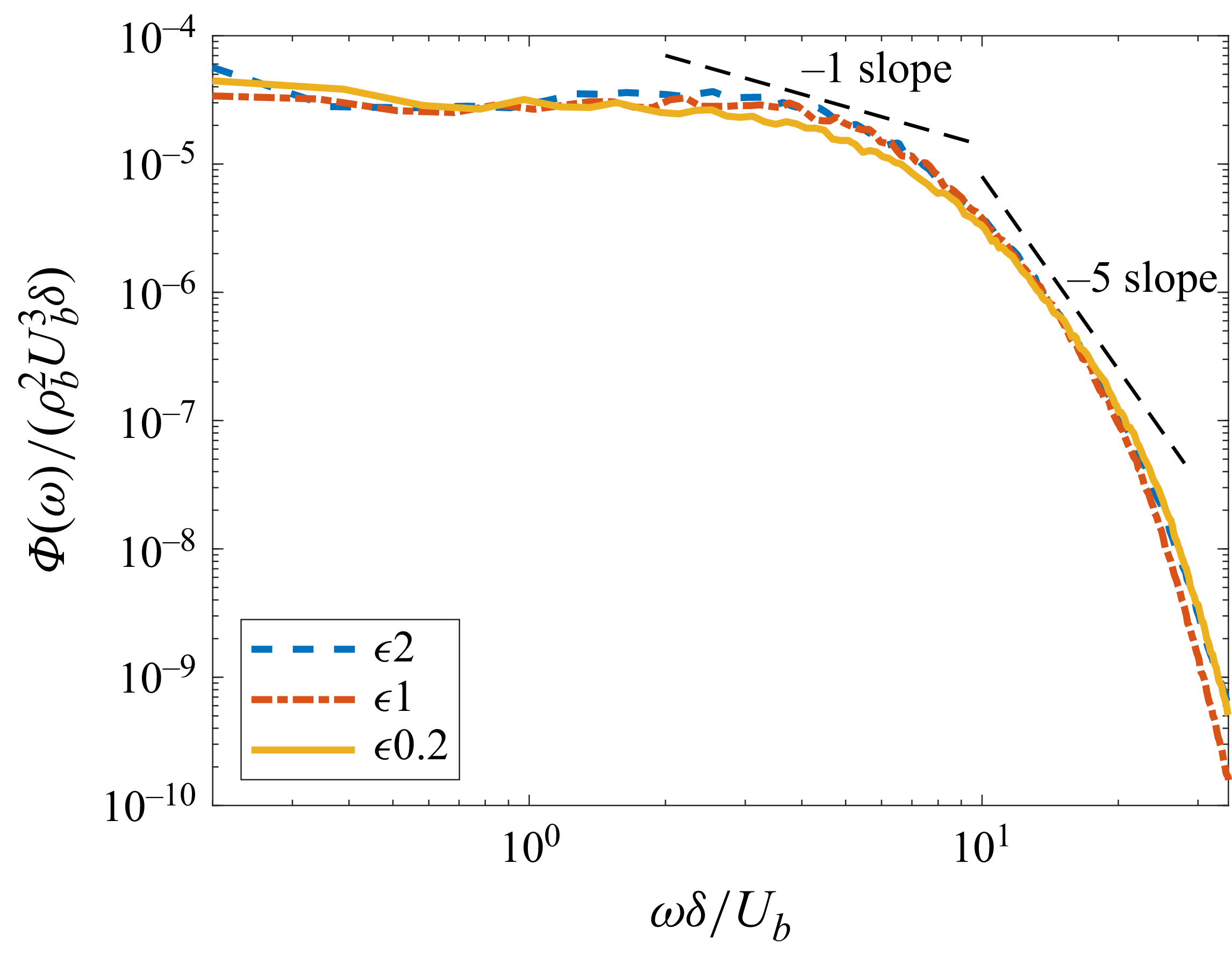
Figure 6 shows the comparison of the one-point temporal spectra of the WPF over cylinders of various diameters. All spectra exhibit a
 $\omega ^{-1}$
scaling in the intermediate regime, but a
 $\omega ^{-5}$
scaling in the high-frequency regime. This is similar to the plane-channel flows (Bull Reference Bull1996; Liu et al. Reference Liu, Wang and Wang2024). Clearly, the spectra of
 $\epsilon =2$
and
 $\epsilon =1$
show minimal difference. This is well known in incompressible studies – when the inner cylinder is large, the effects of curvature on the WPF are negligible (Neves & Moin Reference Neves and Moin1994b
). However, when
 $\epsilon$
reduces to
 $0.2$
, the wall pressure spectrum shows a clear reduction in magnitude in the intermediate frequency regime. At high frequencies, however, the spectral magnitude exhibits a slight increase compared to that at
 $\epsilon =1$
. The effects of curvature on the low-frequency PSD component appear rather limited. Note, however, that this does not contradict the findings of Neves & Moin (Reference Neves and Moin1994b
), where the PSD reduces at all frequencies when the friction velocity
 $u_\tau$
is used for non-dimensionalisation. To examine the structures of the WPF, however, one is more interested in the wavenumber–frequency spectra shown in the following subsections.
Non-dimensionalised PSD
 $\varPhi (\omega )/(\rho _b^2 U_b^3\delta )$
of the WPF over cylinders of various diameters.

4.2. The 1-D wavenumber–frequency spectra
Figures 7(a,b) compare the 1-D wavenumber–frequency spectra
 $\varPhi (k_z, \omega )$
when
 $\epsilon$
varies. At low frequency
 $\bar {\omega }=1$
(defined as
 $\omega \delta / U_b$
as above), one can see a clear dominant peak at the convective wavenumbers
 $\omega /U_c$
. Reducing the radius from
 $\epsilon =2$
to
 $\epsilon=1$
lowers the magnitude at high (including negative) wavenumbers. Further decreasing the cylinder radius to
 $\epsilon =0.2$
reduces the spectra more significantly. However, the magnitude at the convective wavenumber appears virtually unchanged. This implies that the streamwise length scale of the WPF becomes larger, a result in accordance with earlier incompressible studies (Neves & Moin Reference Neves and Moin1994b
). In addition, one starts to see a significant spectral feature change when
 $\epsilon$
reduces to
 $0.2$
, i.e. acoustic peaks (see § 4.3) start to appear in the supersonic wavenumber region.
The 1-D wavenumber–frequency
 $\varPhi (k_z, \omega )/(\rho _b^2 U_b^3 \delta ^2)$
spectra of WPF for various cylinder diameters: (a)
 $\bar {\omega }=1$
,
 $5$
and
 $10$
; (b)
 $\bar {\omega }=15$
,
 $20$
and
 $25$
. The spectral magnitudes at
 $\bar {\omega }=15$
and
 $\bar {\omega }=25$
are multiplied by
 $10^3$
and
 $10^{-3}$
, respectively, for separation clarity.

As the frequency increases to
 $\bar {\omega } = 5$
and
 $10$
, the convection peak moves to higher wavenumbers with reduced magnitudes, consistent with a decaying magnitude against frequency as shown in figure 7(a). The effects of reducing
 $\epsilon$
are similar to those at
 $\bar {\omega } = 1$
, except that the acoustic peaks at
 $\epsilon =0.2$
are increasingly strong as the frequency increases. In addition, the spectra appear to shift to lower wavenumbers as
 $R$
reduces.
The acoustic peaks and spectral shift are more significant at higher frequencies. Figure 7(b) shows the spectra at
 $\bar {\omega }=15$
,
 $20$
and
 $25$
. At
 $\bar {\omega }=15$
, the spectrum is smooth at all wavenumbers at
 $\epsilon =2$
, but starts to show some acoustic peaks at
 $\epsilon = 1$
. At
 $\epsilon =0.2$
, a much denser cluster of acoustic peaks starts to occur. As the frequency increases to
 $\bar {\omega }=20$
and
 $25$
, these acoustic peaks are both stronger and denser. Note that acoustic peaks do not appear in the case of rectangular channels (Liu et al. Reference Liu, Wang and Wang2024), and are caused by the curvature of the walls. Similar to the appearance of the acoustic peaks, the tendency of spectral shift appears increasingly evident as the frequency increases.
4.3. The 2-D wavenumber–frequency spectra
The fact that the spectral peaks observed in figure 7 are acoustics-induced can be clearly seen from the 2-D wavenumber–frequency spectra
 $\varPhi (k_z, m, \omega )$
. Note that the axisymmetric mode (
 $m = 0$
) is of particular importance in practical applications (Crighton et al. Reference Crighton, Dowling, Ffowcs-Williams, Heckl, Leppington and Bartram1992; Liu et al. Reference Liu, Wang and Wang2024). For example, the flow noise measured in sonar arrays is only related to the WPF of mode
 $m=0$
(Crighton et al. Reference Crighton, Dowling, Ffowcs-Williams, Heckl, Leppington and Bartram1992; Dowling Reference Dowling1998). The following analysis therefore focuses primarily on this mode, although higher azimuthal modes are also briefly examined subsequently in figure 12. Figure 8 first shows the contour of
 $\varPhi (k_z, 0, \omega )$
over cylinders of various diameters. Note that the colour is plotted in a logarithmic scale due to the wide span of the spectral magnitude.
The 2-D wavenumber–frequency spectra at (a,d)
 $\epsilon =2$
, (b,e)
 $\epsilon =1$
and (c, f)
 $\epsilon =0.2$
. The dotted lines represent the acoustic duct modes solved from (4.5).

Figure 8. Long description
Panel A: A heat map showing the 2-D wavenumber-frequency spectra. The x-axis is labeled k_z delta ranging from −40 to 40, and the y-axis is labeled Ωδ/U_b ranging from 0 to 40. The color scale on the right indicates values from 10^−18 to 10^−3, with lighter colors representing higher values. The heat map shows a gradient with higher values concentrated towards the bottom right. Panel B: A heat map similar to Panel A, with the same axes and color scale. The pattern is similar, with higher values concentrated towards the bottom right. Panel C: A heat map similar to Panels A and B, with the same axes and color scale. The pattern is consistent with the previous panels. Panel D: A heat map showing the 2-D wavenumber-frequency spectra. The x-axis is labeled k_z delta ranging from −10 to 10, and the y-axis is labeled Ωδ/U_b ranging from 0 to 20. The color scale on the right indicates values from 10^−18 to 10^−3, with lighter colors representing higher values. The heat map shows a gradient with higher values concentrated towards the bottom right, and dotted lines representing acoustic duct modes. Panel E: A heat map similar to Panel D, with the same axes and color scale. The pattern is similar, with higher values concentrated towards the bottom right and dotted lines representing acoustic duct modes. Panel F: A heat map similar to Panels D and E, with the same axes and color scale. The pattern is consistent with the previous panels, with higher values concentrated towards the bottom right and dotted lines representing acoustic duct modes.
Figure 8(a) shows
 $\varPhi (k_z, 0, \omega )$
for
 $\epsilon =2$
. Due to compressibility, we see an evident violation of the Kraichnan–Phillips theorem that demands
 $\varPhi (k_z, k_y, \omega ) \to 0$
as
 $k_z^2+k_y^2 \to 0$
(Ffowcs-Williams Reference Ffowcs-Williams1965), where
 $k_y$
represents the spanwise wavenumber (in the annular duct case,
 $k_y$
is asymptotically equal to
 $m/R$
). Similar to the incompressible case (Neves & Moin Reference Neves and Moin1994b
), the energy of the WPF is dominated by the convective ridges. As the frequency increases, however, these ridges become increasingly wide, suggesting a less well-defined convection velocity. What sets the compressible spectra apart from their incompressible counterparts, however, are a series of discrete curves clearly visible albeit at a much weaker intensity. These are the acoustic modes in annular ducts, which are similar to those in plane-channel flows (Liu et al. Reference Liu, Wang and Wang2024).
To examine these acoustic modes closely, figures 8(d–f) show close-up views of the low-wavenumber regimes of figures 8(a–c). Also included are the analytical dispersion relations of the acoustic modes in annular ducts with uniform mean flow (Crighton et al. Reference Crighton, Dowling, Ffowcs-Williams, Heckl, Leppington and Bartram1992), i.e.
 \begin{equation} \big(\beta ^2 k_z + k M_b\big)^2 = k^2 - \mu _{\textit{mn}}^2\beta ^2, \end{equation}
where
 $\beta ^2 = 1-M_b^2$
and
 $k=\omega / c_\infty$
, and
 $\mu _{\textit{mn}}$
is the
 $n$
th root of
 \begin{equation} J_m^\prime (\mu _{\textit{mn}} R)\, Y_m^\prime (\mu _{\textit{mn}} (R+2\delta )) - J_m^\prime (\mu _{\textit{mn}} (R+2\delta ))\, Y_m^\prime (\mu _{\textit{mn}}R) = 0. \end{equation}
In (4.6),
 $J_m$
and
 $Y_m$
represent the
 $m$
th-order Bessel functions of the first and second kinds, respectively, the prime superscript represents their first derivatives, and
 $n$
denotes an integer representing the radial order of the acoustic mode. One can see the nearly perfect collapse of these predicted duct modes with those discrete curves in figures 8(d–f). Note the striking difference in the spectral magnitudes of these acoustic modes and the convective ridge. However, as
 $\epsilon$
reduces, these acoustic modes appear to intensify, as shown by the increasingly bright lines in figures 8(a–c).
To examine the acoustic modes in detail, we plot their pressure distribution within the annular ducts of various diameters. These acoustic modes can be calculated analytically, and they take the form
 \begin{equation} p=C_{\textit{mn}}\left (Y_m^\prime (\mu _{\textit{mn}}R)\, J_m(\mu _{\textit{mn}}r)- J_m^\prime (\mu _{\textit{mn}}R)\,Y_m(\mu _{\textit{mn}} r)\right ) \exp ({\rm i}m\theta )\exp {(-{\rm i}k_z z)}, \end{equation}
where
 $C_{\textit{mn}}$
represents the normalisation constant that depends on the azimuthal order
 $m$
and radial order
 $n$
. In this paper, we focus on the axisymmetric mode
 $m=0$
, and use (4.7) to plot the acoustic mode propagating towards the
 $+z$
direction. The mode propagating towards the
 $-z$
direction is similar and hence omitted.
Axisymmetric (
 $m=0$
) acoustic modes at
 $k\delta =2$
: (a–c) modes of radial order
 $n=1$
(plane waves); (d–f) modes of radial order
 $n=2$
. Here, (a,d)
 $\epsilon =2$
, (b,e)
 $\epsilon =1$
, (c, f)
 $\epsilon =0.2$
.

Axisymmetric (
 $m=0$
) acoustic modes at
 $k\delta =5$
: (a–c) modes of radial order
 $n=2$
; (d–f) modes of radial order
 $n=3$
. Here, (a,d)
 $\epsilon =2$
, (b,e)
 $\epsilon =1$
, (c, f)
 $\epsilon =0.2$
.

The cross-sections of the duct modes for the three cylinder diameters are shown in figures 9 and 10 at reduced frequencies
 $k\delta =2$
and
 $5$
, respectively. Figures 9(a–c) show the real part of (4.7) for the acoustic mode of radial order
 $n=1$
at
 $k\delta =2$
. These represent plane-wave modes (the straight discrete lines in figure 8) propagating along the
 $+z$
direction. Hence the WPF amplitudes on the inner and outer cylinder walls remain identical. In figure 8, we show that these plane-wave modes appear stronger on the inner cylinder wall as
 $\epsilon$
reduces, and one would therefore expect a similar behaviour on the outer wall.
Figures 9(d–f), on the other hand, show the acoustic modes of the radial order
 $n=2$
. It is worth noting that only two radial orders (
 $1$
and
 $2$
) are cut-on at this reduced frequency
 $k\delta =2$
, while higher-order modes are effectively cut-off. This can be seen clearly from figures 8(d–f) by drawing a horizontal line at
 $\omega \delta /U_b=5$
. From figures 9(d–f), we can see that as the curvature increases, the acoustic pressure on the inner cylinder wall becomes increasingly larger than that on the outer wall. To put this difference into perspective, the acoustic pressure at the inner wall is approximately 10 dB higher than that on the outer wall. One therefore expects less energetic acoustic peaks for the radial order
 $n=2$
on the outer wall.
As the frequency increases, figures 8(d–f) show that more acoustic modes of higher radial orders become cut-on. To show these modes more closely, we choose a higher frequency
 $k\delta =5$
and plot the acoustic duct modes of radial orders
 $2$
and
 $3$
in figure 10. Again, high-order modes are cut-off. As the radial order increases, the acoustic pressure shows more zeros along the radial direction, while the streamwise wavenumber decreases. The latter is expected because of (4.5). Moreover, the difference in the pressure amplitude on the inner and outer walls appears larger as
 $n$
increases. This suggests that the higher-order acoustic peaks in the WPF spectra are increasingly more pronounced on the inner wall than those on the outer wall. Note, however, that although we can examine the behaviour of WPF on the outer walls, our primary concern in practice, and hence in this paper, is the WPF over the inner cylinder walls.
The non-dimensional 2-D wavenumber–frequency spectra
 $\varPhi (k_z, 0, \omega )/(\rho _b^2 U_b^3 \delta ^2)$
over cylinders of various diameters; the spectral magnitudes at
 $\bar {\omega }=15$
and
 $\bar {\omega }=25$
are multiplied by
 $10^3$
and
 $10^{-3}$
, respectively, for separation clarity.

To compare the 2-D wavenumber–frequency spectra over inner walls quantitatively, figure 11(a) shows
 $\varPhi _{pp}(k_z, 0, \omega )$
against
 $k_z\delta$
at
 $\bar {\omega } = 1$
,
 $5$
and
 $10$
. One can see that decreasing the diameter increases the spectral magnitude at low wavenumbers, but decreases it at high wavenumbers. Different from figure 7(b), spectral peaks due to acoustic duct modes can be found at all cylinder diameters. As shown in figure 8, these peak wavenumbers can be well predicted by (4.5). As the frequency increases, the low-wavenumber spectral augmentation appears stronger, as shown in figure 11(b). Note that when
 $\bar {\omega } \geqslant 20$
, the low-wavenumber spectral magnitude at
 $\epsilon =2$
is broadly elevated without apparent peaks, in accordance with Liu et al. (Reference Liu, Wang and Wang2024). But the acoustic peaks continue to show up when
 $\epsilon =1$
and
 $0.2$
. In addition, the acoustic peaks become more clustered because more duct modes are cut-on, as shown straightforwardly in figure 8. Clearly, when all azimuthal modes are summed to obtain
 $\varPhi (k_z, \omega )$
, more spectral peaks will appear, as evidenced by figure 7.
The non-dimensional 2-D wavenumber–frequency spectra
 $\varPhi (k_z, m, \omega )/(\rho _b^2 U_b^3 \delta ^2)$
for azimuthal modes
 $m=0$
,
 $1$
and
 $2$
for
 $\epsilon = 0.2$
; the spectral magnitudes at
 $\bar {\omega }=15$
and
 $\bar {\omega }=25$
are multiplied by
 $10^3$
and
 $10^{-3}$
, respectively, for separation clarity.

Figure 12. Long description
Panel A: A line graph shows the spectral magnitudes for azimuthal modes 0, 1, and 2 at angular frequencies 1, 5, and 10. The x-axis represents the streamwise wavenumber (kzδ) ranging from −30 to 30, and the y-axis represents the spectral magnitude (Φ(kz, m, Ω))/(ρ²U³δ²) on a logarithmic scale from 10^−¹^6 to 10^−^4. Different line styles and colors distinguish the modes and frequencies. Panel B: Another line graph displays spectral magnitudes for azimuthal modes 0, 1, and 2 at angular frequencies 15, 20, and 25. The x-axis represents the streamwise wavenumber (kzδ) ranging from −20 to 30, and the y-axis represents the spectral magnitude (Φ(kz, m, Ω))/(ρ²U³δ²) on a logarithmic scale from 10^−¹^8 to 10^−^4. The spectral magnitudes at m = 0 and m = 1 are multiplied by 10³ and 10^−³, respectively, for separation clarity. Different line styles and colors distinguish the modes and frequencies.
To show the variation of the wavenumber–frequency spectra against azimuthal modes, figure 12 shows the spectra at various
 $m$
for
 $\epsilon =0.2$
. When the frequency is low (
 $\bar {\omega }=1$
), one can see that only the spectra at
 $m=0$
exhibit acoustic peaks, since high-order modes are effectively cut-off according to (4.5). The spectral magnitude outside the acoustic peaks remains approximately identical. As the frequency increases to 5 and 10, acoustic modes at
 $m=1$
and
 $m=2$
become cut-on. As the frequency further increases, more acoustic modes are cut-on and appear in the spectra shown in figure 12(b). Note that the elevated magnitude in the supersonic region appears to exist for all
 $m$
. Other than that, the spectra look similar elsewhere.
5. Analytical modelling of the low-wavenumber WPF augmentation
The low-wavenumber augmentation in spectral magnitude as
 $\epsilon$
reduces is of great concern in practical applications such as towed sonar arrays (Bull Reference Bull1996). To understand why such augmentation occurs, we start from modelling the WPF generated by a homogeneous turbulent boundary layer over an infinitely long cylinder. Note that such a model is not strictly applicable to the present set-up, where channel flows within concentric annular ducts are simulated instead of free boundary layers. Nevertheless, we expect the effects of curvature on the WPF in these two cases to remain similar, particularly at low wavenumbers. Therefore, we attempt to discuss the low-wavenumber WPF augmentation via modelling the boundary layer case.
5.1. Modelling WPF based on the Lighthill acoustic analogy
Using the Lighthill acoustic analogy and the acoustic Green’s function, the WPF spectrum beneath a homogeneous turbulent boundary layer over an infinitely long cylinder can be found analytically as (Dhanak Reference Dhanak1988; Crighton et al. Reference Crighton, Dowling, Ffowcs-Williams, Heckl, Leppington and Bartram1992)
 \begin{equation} \hat {p}(k_z, m, \omega ) = \int T_{\textit{ij}}(\boldsymbol{y}, \tau ) \frac {\partial ^2 }{\partial y_i\, \partial y_j} \left ( -\frac {1}{\alpha R} \frac {H_m^{(1)}(\alpha \sigma )}{H_m^{(1)\prime }(\alpha R)}\, \mathrm{e}^{{\rm i} k_z y_3}\, \mathrm{e}^{{\rm i} m \phi }\, \mathrm{e}^{-{\rm i} \omega \tau } \right ) {\rm d}^3 \boldsymbol{y} \,\mathrm{d} \tau , \end{equation}
where
 $\boldsymbol{y}\equiv (y_1, y_2, y_3)$
denotes the Cartesian coordinates of the source position,
 $\tau$
is the source time,
 $T_{\textit{ij}}$
(
 $i,j=1,2,3$
) is the Lighthill stress tensor,
 $\alpha = \sqrt {\omega ^2/c_\infty ^2 - k_z^2}$
,
 $H_m^{(1)}(z)$
is the
 $m$
th-order Hankel function of the first kind, and
 $(\sigma , \phi , y_3)$
are the corresponding coordinates of
 $\boldsymbol{y}$
in the cylindrical frame shown in figure 2, i.e.
 $\sigma =\sqrt {y_1^2+y_2^2}$
,
 $\phi =\arccos y_2/\sigma$
. The spatial integration in (5.1) is performed within the entire boundary layer over the cylinder.
The 0th-order mode is of particular relevance, and in the cylindrical coordinates shown in figure 2, it reduces to
 \begin{align} \int _R^{R+\delta } \left [ \frac {-\alpha H_0^{(1)\prime \prime }(\alpha \sigma )} {H_0^{(1)\prime }(\alpha R)}\hat {T}_{r r} -\frac {H_0^{(1)\prime } (\alpha \sigma )}{H_0^{(1)\prime }(\alpha R)} \left ( \frac {\hat {T}_{\theta \theta }}{\sigma } + 2\mathrm{i} k_z \hat {T}_{r z}\right ) \right . \left . + \frac {k_z^2 H_0^{(1)}(\alpha \sigma )}{\alpha H_0^{(1)\prime }(\alpha R)} \hat {T}_{zz} \right ] \frac {\sigma }{R} \,\mathrm{d} \sigma , \end{align}
where the integral along the radial direction
 $\sigma$
is from the cylinder radius
 $R$
to the edge of the boundary layer
 $R+\delta$
, while
 $\hat {T}_{\textit{ij}}$
is the Fourier transform of the Lighthill stress tensor, given by
 \begin{equation} \hat {T}_{\textit{ij}}(\sigma , k_z, 0, \omega ) = \iint T_{\textit{ij}}(\sigma , y_1, \phi , \tau )\, \mathrm{e}^{{\rm i} k_z y_3}\, \mathrm{e}^{-{\rm i} \omega \tau }\,\mathrm{d} y_3 \,\mathrm{d} \phi \,\mathrm{d} \tau , \end{equation}
with the subscripts
 $i$
and
 $j$
taking the values of
 $r$
,
 $\theta$
and
 $z$
in the cylindrical coordinates shown in figure 2. Equation (5.2) shows that the
 $0$
th-order WPF are only generated by the stress terms
 $\hat {T}_{\textit{rr}}$
,
 $\hat {T}_{\theta \theta }$
,
 $\hat {T}_{r z}$
and
 $\hat {T}_{zz}$
within the boundary layer, and are independent of
 $\hat {T}_{\theta r}$
and
 $\hat {T}_{z\theta }$
. The latter two components are also expected to be small (see e.g. Appendix A for more details).
In the vicinity of the sonic peak
 $k_z = \omega / c_\infty$
, the last term in (5.2) is singular, but integrable. In practice, the height of these sonic peaks is regularised by the finite size and mean-flow refraction effects of the boundary layer (Bull Reference Bull1996), details of which are not discussed here. Note that in the channel flow case, more spectral peaks are expected apart from the sonic peak because of the presence of multiple cut-on duct modes. In most applications where the low-wavenumber components are of particular concern, one often has
 $k_z r \ll 1$
(
 $r$
takes a value between
 $R$
and
 $R+\delta$
). In such cases, the last two terms of (5.2) can be neglected except near the sonic singularity.
When the cylinder radius and boundary layer thickness are compact (
 $kR \ll 1$
and
 $k\delta \ll 1$
; note that
 $k$
represents the acoustic wavenumber
 $\omega /c_\infty$
), e.g. for classical applications in towed sonar arrays, (5.2) can be approximated using the small-argument expansion of the Hankel functions as (Crighton et al. Reference Crighton, Dowling, Ffowcs-Williams, Heckl, Leppington and Bartram1992)
 \begin{align} \hat {p}(k_z, 0, \omega ) \approx &\int _0^1\frac {\hat {T}_{r r} - \hat {T}_{\theta \theta } }{\epsilon +h} \,\mathrm{d} h, \end{align}
where
 $h\equiv (\sigma -R)/\delta$
represents the non-dimensionalised radial distance measured from the inner cylinder wall, and therefore takes values from
 $0$
to
 $1$
. On the other hand, when the cylinder radius is sufficiently non-compact (e.g. at sufficiently high frequencies), i.e.
 $kR \gg 1$
, the Hankel functions can be expanded using their asymptotic form, and (5.2) at low wavenumbers can be approximated as
 \begin{align} \hat {p}(k_z, 0, \omega ) \approx &\int _0^1 \left [\sqrt {1+\frac {h}{\epsilon }}\, \alpha \delta\, \mathrm{e}^{{\rm i} \alpha \delta h}\, \mathrm{e}^{-{\rm i}{\pi }/{2}}\, \hat {T}_{\textit{rr}} - \frac {1}{\sqrt {\epsilon (\epsilon +h)}}\, \mathrm{e}^{{\rm i} \alpha \delta h }\, \hat {T}_{\theta \theta }\right ] \mathrm{d} h. \end{align}
Assuming that the distributions of Lighthill stress tensors
 $\hat {T}_{\textit{rr}}$
and
 $\hat {T}_{\theta \theta }$
between
 $h=0$
and
 $h=1$
do not change significantly as
 $R$
varies, (5.4) and (5.5) show that the
 $0$
th-order spectrum at small
 $k_z$
would increase when the radius of the inner cylinder reduces. This complies with the low-wavenumber increase of
 $\varPhi (k_z, 0, \omega )$
observed at both low and high frequencies in figure 11. Note that the
 $\epsilon$
terms in (5.4) and (5.5) result from the asymptotic approximation of Hankel functions rather than from the Lighthill stress. This suggests that the low-wavenumber increase is a ‘geometric’ effect connected with the Green’s function.
In particular, the appearance of
 $1/\sqrt {\epsilon (\epsilon +h)}$
in (5.5) as opposed to
 $1/(\epsilon +h)$
in (5.4) suggests that the amplification at high frequencies may be more pronounced than that at low frequencies. There exists indeed such a tendency in figure 11 as the frequency increases. Note that only radial and azimuthal velocity disturbances appear important. Moreover, both (5.4) and (5.5) suggest that as the curvature increases, disturbances close to the wall are increasingly important in generating low-wavenumber components of the WPF spectrum. This complies with the fact that the convective velocity at a fixed
 $\omega \delta / u_\tau$
decreases as
 $R$
reduces. This signals a potential for low-wavenumber WPF control using near-wall treatment on thin cylinders.
5.2. Comparison with DNS
In the derivation reaching (5.4) and (5.5), the assumption that the Lighthill stress tensors
 $\hat {T}_{\textit{rr}}$
and
 $\hat {T}_{\theta \theta }$
between the cylinder wall (
 $h=0$
) and outer edge of the boundary layer (
 $h=1$
) do not change significantly as
 $R$
varies is important. To examine to what extent this assumption remains valid, we first show the distribution of the two stress components along the wall-normal direction at fixed frequency
 $\omega$
and wavenumber
 $k_z$
. To do that, similar to (4.2), we calculate
 $\varPsi _{r r}(\sigma , k_z, 0, \omega )$
and
 $\varPsi _{\theta \theta }(\sigma , k_z, 0, \omega )$
, i.e. the wavenumber–frequency spectra of
 $\hat {T}_{\textit{rr}}(\sigma , k_z, 0, \omega )$
and
 $\hat {T}_{\theta \theta }(\sigma , k_z, 0, \omega )$
, respectively, and show their distributions along
 $h$
in wall units (
 $h^+=h\delta u_\tau /\nu$
). Note that the wavenumber–frequency spectra satisfy
 $\varPsi _{\textit{rr}} \propto |\hat {T}_{\textit{rr}}|^2$
while
 $\varPsi _{\theta \theta } \propto |\hat {T}_{\theta \theta }|^2$
, therefore,
 $\sqrt {\varPsi _{\textit{rr}}}$
and
 $\sqrt {\varPsi _{\theta \theta }}$
are shown in figures 13–16.
As mentioned above, we focus on the low-wavenumber region, where
 $k_z r \ll 1$
(
 $r$
takes values between
 $R$
and
 $R+\delta$
). However, the streamwise wavenumber resolution of the present simulation is only
 $k_z \delta \approx 0.125$
. This implies that the minimum non-zero wavenumber that can be resolved corresponds to a value of
 $k_z r$
up to approximately
 $0.4$
. Therefore, we only show
 $\sqrt {\varPsi _{r r}}$
and
 $\sqrt {\varPsi _{\theta \theta }}$
at
 $k_z\delta =0$
in this paper. Nevertheless, doing this does not reduce much generality, because the wavenumber–frequency spectrum has a well-known wavenumber white behaviour (Bull Reference Bull1996) near
 $k_z\delta =0$
, i.e.
 $\varPhi (k_z, m, \omega )$
obtains a nearly constant value in the low-wavenumber range centring around
 $k_z\delta =0$
.
Note that the asymptotic form of (5.4) requires the cylinder to be acoustically compact, i.e.
 $kR \ll 1$
and
 $k\delta \ll 1$
. This corresponds to a low-frequency range, which we can properly resolve with frequency resolution
 $\omega \delta / U_b\approx 0.165$
(
 $k\delta \approx 0.066$
). However, the asymptotic form of (5.5) requires acoustic non-compactness, i.e.
 $kR \gg 1$
. This implies a considerably high frequency range. To put this into perspective, for
 $\epsilon =0.2$
, a typical number
 $kR=10$
corresponds to frequency
 $\omega \delta / U_b =125$
. Resolving such a frequency needs a very high sampling rate of the flow snapshots, and in practice, storing this large amount of data is very expensive. More importantly, in practical applications, it is the low frequencies that are of our primary concern. As such, in the following, we focus on examining the distribution of
 $\sqrt {\varPsi _{r r}}$
and
 $\sqrt {\varPsi _{\theta \theta }}$
at low frequencies where the cylinder is acoustically compact.
Wall-normal distributions of the Lighthill stress components (a)
 $\hat {T}_{\textit{rr}}$
and (b)
 $\hat {T}_{\theta \theta }$
over the inner cylinder surface at
 $k_z\delta =0$
and
 $\omega \delta /U_b=0$
.

Wall-normal distributions of the Lighthill stress components (a)
 $\hat {T}_{\textit{rr}}$
and (b)
 $\hat {T}_{\theta \theta }$
over the inner cylinder surface at
 $k_z\delta =0$
and
 $\omega \delta /U_b\approx 0.165$
.

Wall-normal distributions of the Lighthill stress components (a)
 $\hat {T}_{\textit{rr}}$
and (b)
 $\hat {T}_{\theta \theta }$
over the inner cylinder surface at
 $k_z\delta =0$
and
 $\omega \delta /U_b\approx 0.33$
.

Wall-normal distributions of the Lighthill stress components (a)
 $\hat {T}_{\textit{rr}}$
and (b)
 $\hat {T}_{\theta \theta }$
over the inner cylinder surface at
 $k_z\delta =0$
and
 $\omega \delta /U_b\approx 1.16$
.

Figure 16. Long description
Two line graphs depict wall-normal distributions of Lighthill stress components over the inner cylinder surface. Panel A: The line graph shows the distribution of the Lighthill stress component with the vertical axis labeled as the square root of the component normalized by specific parameters, ranging from 0 to 6 times 10 to the power of −4. The horizontal axis is labeled as h+ and ranges from 0 to 150. Three lines are plotted for different values of epsilon (2, 1, and 0.2), represented by solid black, dashed blue, and dotted red lines respectively. The trends show varying peaks and behaviors for each epsilon value. Panel B: The line graph shows the distribution of another Lighthill stress component with the vertical axis labeled as the square root of the component normalized by specific parameters, ranging from 0 to 1.4 times 10 to the power of −3. The horizontal axis is labeled as h+ and ranges from 0 to 150. Three lines are plotted for different values of epsilon (2, 1, and 0.2), represented by solid black, dashed blue, and dotted red lines respectively. The trends show varying peaks and behaviors for each epsilon value.
Figure 13 shows the amplitude spectra of
 $\hat {T}_{\textit{rr}}(\sigma , 0, 0, 0)$
and
 $\hat {T}_{\theta \theta }(\sigma , 0, 0, 0)$
. These are the steady and homogeneous components of the Lighthill stress tensors, and should be more properly interpreted as propagation effects rather than as a source in the acoustic analogy framework. Nevertheless, we see that as curvature increases, the two steady stress components generally decrease in amplitude. However, they do not differ from each other by orders of magnitude. In terms of decibels, the difference in their amplitudes is limited to 3 dB.
The distribution at
 $k_z \delta =0$
and
 $\omega \delta / U_b \approx 0.165$
, as demonstrated in figure 14, shows a similar story. However, it is worth noting that the amplitude becomes much smaller than that at
 $\omega \delta /U_b=0$
. Such a trend further continues as frequency increases, as shown in figures 15 and 16, with non-dimensional frequencies
 $\omega \delta / U_b \approx 0.33$
and
 $1.16$
, respectively. This is consistent with the fact that the low-wavenumber WPF decrease quickly as frequency increases. Unlike figures 13 and 14, figures 15 and 16 show that the amplitudes of
 $\hat {T}_{\theta \theta }$
and
 $\hat {T}_{\textit{rr}}$
largely increase as the curvature increases. However, the difference is not significant. Distributions of these two stress components at even higher frequencies are shown in Appendix B. It is worth noting that as frequency increases, the Lighthill stress components appear to converge increasingly less satisfactorily.
We can now calculate both
 $\hat {T}_{\textit{rr}}$
and
 $\hat {T}_{\theta \theta }$
, and predict the wavenumber–frequency spectra of the WPF using (5.4). Note that the model developed in this section is for the WPF beneath a homogeneous turbulent boundary layer; therefore, it is not strictly applicable to the present channel flows. Nevertheless, we can still compare the model prediction with the simulation results, hoping to capture the important trend instead of seeking an exact agreement.
Results are shown in figure 17, where the predicted WPF wavenumber–frequency spectra
 $\varPhi (k_z, m, \omega )$
for the axisymmetric (
 $m=0$
) mode at low frequencies are compared with DNS results. Again, since we are primarily interested in low wavenumbers where the WPF has a wavenumber white behaviour near
 $k_z\delta =0$
, we show the spectrum
 $\varPhi (0, 0, \omega )$
as a function of
 $\omega$
. The predicted spectra are obtained from (5.4) using
 $\hat {T}_{\textit{rr}}$
and
 $\hat {T}_{\theta \theta }$
examined in figures 13–16. From figure 17, we can see that spectral augmentation as
 $\epsilon$
decreases is well predicted from the asymptotic equation. As
 $\epsilon$
decreases from
 $2$
to
 $0.2$
, the amplitude of the DNS WPF spectra increases by almost two orders of magnitude. This trend is well captured in the prediction. Considering that
 $\hat {T}_{r r}$
and
 $\hat {T}_{\theta \theta }$
do not change significantly as
 $\epsilon$
varies, this augmentation is indeed primarily contributed by the
 $\epsilon +h$
term in (5.4).
In addition, outside the acoustic peaks, the predicted spectra follow the variation trend of the DNS results correctly. The agreement is slightly better for
 $\epsilon =2$
and
 $\epsilon =1$
, while the spectrum of
 $\epsilon =0.2$
is slightly over-predicted. Note that a modest decrease in the upper limit of the integral in (5.4) reduces the predicted
 $\varPhi$
amplitude significantly for
 $\epsilon =2$
and
 $1$
, but the variation is negligible for
 $\epsilon =0.2$
. This is a direct demonstration that disturbances closer to the wall are increasingly important in generating WPF as the inner cylinder becomes thinner. Considering that the model does differ from the channel flow set-up, such an agreement is sufficient to show the validity of (5.4).
Comparison of the WPF wavenumber–frequency spectrum
 $\varPhi (0, 0, \omega )/(\rho _b^2 U_b^3 \delta ^2)$
between the asymptotic prediction and DNS results.

6. Conclusion and future work
Compressible DNS simulations within concentric annular ducts are performed in this paper to study the effects of curvature on the WPF characteristics over cylindrical walls. The inner cylinder radius
 $R$
ranges from
 $0.2\delta$
,
 $\delta$
,
 $2\delta$
to
 $\infty$
. The simulations are validated against previous results in the literature, and the effects of curvature on the flow statistics are discussed. It is found that as the curvature increases, the three normal Reynolds stress components, together with
 $\langle u_r^{\prime +}u_z^{\prime +}\rangle$
, over the inner cylinder wall decrease and peak slightly closer to the wall. However, the flows over the outer cylinder wall show an opposite behaviour.
Regarding the WPF, results show that as
 $R$
decreases, the magnitude of the one-point PSD of the WPF decreases at intermediate frequencies but increases at high frequencies. The magnitude of the 1-D streamwise wavenumber–frequency spectrum decreases at high wavenumbers. Moreover, as
 $R$
reduces to
 $0.2\delta$
, the spectra start to show acoustic peaks at low wavenumbers, which become increasingly strong at higher frequencies. These acoustic peaks represent acoustic duct modes within the concentric annular channel. An examination of these modes shows that the plane-wave mode (first-order radial mode) does not discriminate between the inner and outer walls in terms of pressure amplitude; however, modes of higher radial orders are more energetic on the inner walls.
The 0th-order 2-D wavenumber–frequency spectrum is of great importance in practical applications. The DNS show that reducing
 $R$
decreases the high-wavenumber components but increases the low-wavenumber components. In particular, the low-wavenumber increase appears stronger at high frequencies. Analytical modelling based on the Lighthill acoustic analogy shows that this arises primarily from the ‘geometric’ effects connected with the Green’s function. The asymptotic prediction of this model captures the low-wavenumber spectral augmentation observed in the DNS at low frequencies correctly, though quantitative differences remain due to the modelling assumptions. The 0th-order low-wavenumber WPF are generated mainly by azimuthal and radial disturbances. Moreover, disturbances close to the wall play an increasingly important role in generating WPF as the curvature increases. This is important as it suggests a possibility of low-wavenumber WPF control using wall treatments. At
 $R=0.2\delta$
, 2-D wavenumber–frequency spectra of higher azimuthal orders are virtually identical to the 0th-order spectra except near the acoustic ridges.
The present work mainly focuses on the effects of curvature on the WPF characteristics. The effects of Mach number are examined in Liu et al. (Reference Liu, Wang and Wang2024) for rectangular channels. It is, however, worth studying how these effects change in the annular channel. The difference in WPF between channel flows and free boundary layers also warrants investigation. These points form part of our future work.
Acknowledgements
The authors wish to thank Professor R.D. Sandberg for the licence to use the code HiPSTAR, and Professor M. Wang for inspiring discussions on compressible DNS simulations.
Funding
The authors wish to gratefully acknowledge the National Natural Science Foundation of China under grant nos. 12472263, U2570222, 12432010, 12588201 and 12572247.
Declaration of interests
The authors report no conflict of interest.
Appendix A. Distribution of other Reynolds stress components
The wall-normal distribution of the other two Reynolds stress components, i.e.
 $\langle u_z^{\prime +} u_\theta ^{\prime +}\rangle$
and
 $\langle u_r^{\prime +} u_\theta ^{\prime +}\rangle$
, over the inner and outer cylinder walls are shown in figure 18. Figures 18(a) and 18(b) show the two components over the inner wall. First, as expected, both
 $\langle u_z^{\prime +} u_\theta ^{\prime +}\rangle$
and
 $\langle u_r^{\prime +} u_\theta ^{\prime +}\rangle$
are two orders of magnitude smaller than other Reynolds stress components, while the former appears larger than the latter. In addition, the plane-channel flow appears to have the largest value. The wall-normal distributions over the outer cylinder wall, as shown in figures 18(c) and 18(d), are generally similar. It is also worth mentioning that neither component contributes to the 0th-order WPF wavenumber–frequency spectra, as shown in § 5.
Wall-normal distributions of the Reynolds stresses of (a)
 $\langle u^{\prime +}_zu^{\prime +}_\theta \rangle$
and (b)
 $\langle u^{\prime +}_ru^{\prime +}_\theta \rangle$
over the inner cylinder wall, and (c)
 $\langle u^{\prime +}_z u^{\prime +}_\theta \rangle$
and (d)
 $\langle u^{\prime +}_r u^{\prime +}_\theta \rangle$
over the outer cylinder wall.

Figure 18. Long description
Panel A: A line graph shows the wall-normal distribution of Reynolds stress with the y-axis labeled as 〈u_z’+u_θ’〉 and the x-axis labeled as y+. The graph includes four lines representing different values of ε (infinity, 2, 1, and 0.2). Panel B: A line graph shows the wall-normal distribution of Reynolds stress with the y-axis labeled as 〈u_r’+u_θ’〉 and the x-axis labeled as y+. The graph includes four lines representing different values of ε (infinity, 2, 1, and 0.2). Panel C: A line graph shows the wall-normal distribution of Reynolds stress with the y-axis labeled as 〈u_z’+u_θ’〉 and the x-axis labeled as y+. The graph includes four lines representing different values of ε (infinity, 2, 1, and 0.2). Panel D: A line graph shows the wall-normal distribution of Reynolds stress with the y-axis labeled as 〈u_r’+u_θ’〉 and the x-axis labeled as y+. The graph includes four lines representing different values of ε (infinity, 2, 1, and 0.2).
Wall-normal distributions of the Lighthill stress components (a)
 $\hat {T}_{\textit{rr}}$
and (b)
 $\hat {T}_{\theta \theta }$
over the inner cylinder surface at
 $k_z\delta =0$
and
 $\omega \delta / U_b=\pi$
.

Appendix B. Distribution of other Lighthill stress components
To further examine the assumption that
 $\hat {T}_{\theta \theta }$
and
 $\hat {T}_{\textit{rr}}$
do not change significantly as curvature varies at relatively higher frequencies, we also show the distribution of them at
 $\omega \delta /U_b=\pi$
and
 $2\pi$
in figures 19 and 20, respectively. These correspond to
 $k\delta$
values
 $1.26$
and
 $2.51$
, respectively, reaching the validity limit of acoustic compactness. The case
 $\omega \delta / U_b=\pi$
shown in figure 19 is similar to that in figure 16, where the amplitudes of
 $\hat {T}_{\textit{rr}}$
and
 $\hat {T}_{\theta \theta }$
grow larger when
 $\epsilon =0.2$
. However, the difference is not significant. Examining these distributions at
 $\omega \delta / U_b=2\pi$
in figure 20, we note first that the amplitudes of both components have decayed significantly to
 $10^{-5}$
. In addition, one can see that as curvature increases, both
 $\hat {T}_{\theta \theta }$
and
 $\hat {T}_{\textit{rr}}$
increase only slightly. The difference between them is small.
Wall-normal distributions of the Lighthill stress components (a)
 $\hat {T}_{\textit{rr}}$
and (b)
 $\hat {T}_{\theta \theta }$
over the inner cylinder surface at
 $k_z\delta =0$
and
 $\omega \delta / U_b=2\pi$
.

The oscillatory behaviour of the curves in figure 20 reflects the limited statistical convergence of the Fourier-transformed Lighthill stress tensor at these very small amplitudes. Despite these oscillations, the key observation, that these Lighthill stress components do not differ by orders of magnitude across different
 $\epsilon$
values, remains valid. From figure 13 to figure 20, it is clear that these Lighthill stress components indeed do not differ significantly in the low-frequency regimes.
 ω
 ky=0
 kz
 Ni
 Δi+
 i
 i
 θ
 r
 z

 θ
 r
 z

 ϵ=0.22

 ⟨uz′+uz′+⟩
 ⟨ur′+ur′+⟩
 ⟨uθ′+uθ′+⟩
 ⟨uz′+ur′+⟩

 ⟨uz′+uz′+⟩
 ⟨ur′+ur′+⟩
 ⟨uθ′+uθ′+⟩
 ⟨uz′+ur′+⟩
 Φ(ω)/(ρb2Ub3δ)

 Φ(kz,ω)/(ρb2Ub3δ2)
 ω¯=1
 5
 10
 ω¯=15
 20
 25
 ω¯=15
 ω¯=25
 103
 10−3

 ϵ=2
 ϵ=1
 ϵ=0.2

 m=0
 kδ=2
 n=1
 n=2
 ϵ=2
 ϵ=1
 ϵ=0.2

 m=0
 kδ=5
 n=2
 n=3
 ϵ=2
 ϵ=1
 ϵ=0.2

 Φ(kz,0,ω)/(ρb2Ub3δ2)
 ω¯=15
 ω¯=25
 103
 10−3

 Φ(kz,m,ω)/(ρb2Ub3δ2)
 m=0
 1
 2
 ϵ=0.2
 ω¯=15
 ω¯=25
 103
 10−3

 T^rr
 T^θθ
 kzδ=0
 ωδ/Ub=0

 T^rr
 T^θθ
 kzδ=0
 ωδ/Ub≈0.165

 T^rr
 T^θθ
 kzδ=0
 ωδ/Ub≈0.33

 T^rr
 T^θθ
 kzδ=0
 ωδ/Ub≈1.16

 Φ(0,0,ω)/(ρb2Ub3δ2)

 ⟨uz′+uθ′+⟩
 ⟨ur′+uθ′+⟩
 ⟨uz′+uθ′+⟩
 ⟨ur′+uθ′+⟩

 T^rr
 T^θθ
 kzδ=0
 ωδ/Ub=π

 T^rr
 T^θθ
 kzδ=0
 ωδ/Ub=2π


