Understanding how legislative institutions condition the translation of individual legislators’ wants into enacted legislation has been a central area of research over the past several decades. In recent years scholars have proposed theories of legislative politics (e.g., Cox and McCubbins Reference Cox and McCubbins2005; Krehbiel Reference Krehbiel1998) that make clear predictions about how changes in the policy preferences of key institutional actors will influence policy outcomes. However, the literature contains almost no direct tests of these predictions because it is difficult to identify the locations of policy status quos in terms of legislators’ policy preferences. In this article, I apply a novel approach able to estimate policy status quo locations across legislative sessions. The estimation strategy uses legislators’ survey responses in conjunction with their roll call votes to identify the ideological position most likely associated with a preference for no policy change—the status quo. I use these estimates to test predictions made by prominent theories of legislative politics for the U.S. Congress from 1994 through 2008.

The past decade has seen an extended debate between advocates of contending models of legislative politics. Pivotal politics theorists argue that institutional rules such as the filibuster and the presidential veto constrain action by floor majorities in the U.S. Congress, but that parties are epiphenomena with little influence on legislative outcomes (Krehbiel Reference Krehbiel1998). In contrast, partisan theories (e.g., Chiou and Rothenberg Reference Chiou and Rothenberg2003; Cox and McCubbins Reference Cox and McCubbins2005; Rhode Reference Rohde1991) contend that parties have substantial real power to make and/or block policy change. The partisan and pivotal models make clear and conflicting predictions concerning policy outcomes and legislative gridlock.

Despite the clarity of the theories, previous studies have not been able to provide direct evidence that partisan (or pivotal) theories do a better job of explaining policy outcomes. Because the locations of the current policy “status quo” and of bills proposed to change the status quo are not well identified in spatial models of roll call voting (Poole Reference Poole2005; Poole and Rosenthal Reference Poole and Rosenthal2007), previous tests of pivotal politics and partisan policy predictions have used indirect measures.

Indirect tests in the literature have produced contradictory and ambiguous results. The results of some previous tests support partisan theories, whereas others have rejected both partisan and pivotal theories, and still others support pivotal politics. Indirect tests by Chiou and Rothenberg (Reference Chiou and Rothenberg2003) rely on gridlock rates. They report evidence consistent with their party unity model. Tests by Covington and Bargen (Reference Covington and Bargen2004) rely on a measure of the percentage of the time conservatives “win” in Congress. They find evidence for majority party effects. Cox and McCubbins (Reference Cox and McCubbins2005) also examine the direction of policy movement in the U.S. House of Representatives, finding a pattern consistent with the party cartel model. Lawrence, Maltzman, and Smith (Reference Lawrence, Maltzman and Smith2006) assume a uniform distribution of initial status quo locations and use this to derive predictions concerning the composition of legislative majorities. Their results favor a majority party agenda-setting model. Krehbiel, Meirowitz, and Woon (Reference Krehbiel, Meirowitz, Woon, Austen-Smith and Duggan2005) examine theoretical predictions concerning the distribution of roll call cut points. Although they find stronger evidence against the pivotal politics model, they note that the party gate-keeping model faces less risk in their tests. Clinton (Reference Clinton2007) attempts to use roll call cut points to infer the nature of the legislative process, but encounters ambiguous results. Stiglitz and Weingast (Reference Stiglitz and Weingast2010) examine the distribution of cut points and variation in the uncertainty with which legislators’ preferences are estimated in an analysis of votes taken in the U.S. House of Representatives. They find shifts in cut points consistent with a partisan model. Saeki (Reference Saeki2009) finds evidence that the policy preferences of veto players (but not their partisan identities) influence the prevalence of gridlock.

This article presents a novel method able to identify status quo locations across time. The resulting status quo estimates from the 103rd through 110th Congress are used to test the pivotal politics (Krehbiel Reference Krehbiel1998) and party cartel (Cox and McCubbins Reference Cox and McCubbins2005) models of congressional lawmaking. These tests are much sharper and more direct than any previous tests in the literature. The empirical analysis provides evidence that both parties and pivots influence policy outcomes and legislative gridlock in Congress. The best-fitting model is one in which the majority and minority parties are able to exert pressure on pivotal members of their caucuses to prevent policy changes that would otherwise have taken place.

MEDIAN, PIVOTAL, AND PARTISAN PREDICTIONS

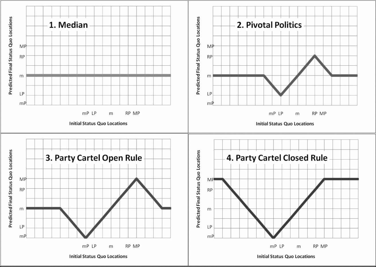
This study uses status quo estimates to test four models of legislative politics: (1) the median voter model, (2) the pivotal politics model (Krehbiel Reference Krehbiel1998), (3) an open rule version of the party cartel model (modified from that proposed by Cox and McCubbins Reference Cox and McCubbins2005), and (4) a closed rule version of the party cartel model (Chiou and Rothenberg Reference Chiou and Rothenberg2003; Cox and McCubbins Reference Cox and McCubbins2005). Comparing the partisan models with the pivotal politics model provides a basis for judging whether parties add to our understanding of legislative outcomes in Congress. Comparing the partisan models with each other provides a basis for evaluating the nature and scope of party influence. Each model makes a set of distinct predictions concerning the distribution of status quo locations, the degree to which particular status quo will change, and the final policies selected when status quo are altered. I discuss each model in turn. Figure 1 illustrates how each model relates initial status quo locations to predicted final status quo locations. Appendix A provides outcome-mapping functions for each model.

FIGURE 1.

Mapping Initial Status Quo to Predicted Outcomes: Expectations for Gridlock and Policy Change in the Median, Pivotal Politics, and Party Cartel Models of Lawmaking

Key: LP, left pivot; m, floor median; RP, right pivot; MP, majority party median (assumed to be on right); mP, minority party median.

Note: Hypothetical preferences. In each subfigure, a positive (45-degree) slope indicates a region in which the status quo remains unchanged because it is gridlocked or blocked.

The simplest model of legislative politics examined here is the median model in which the floor median of each legislative chamber determines policy choices in that chamber. Under bicameralism, policy outcomes are the result of compromise between the chamber medians such that all policies will be moved to locations at or between the ideal points of the House and Senate medians. Although the bicameral core typically includes multiple points, I assume that bicameral negotiation always produces an outcome at the location of the chamber median closest to the original status quo in order to simplify calculation of predicted outcomes (Hammond and Miller Reference Hammond and Miller1987).

The pivotal politics model (Brady and Volden Reference Brady and Volden1998; Krehbiel Reference Krehbiel1998) modifies the median voter model by adding veto players who can prevent enactment of policy change favored by the medians. Krehbiel examines the presidential veto, the two-thirds threshold needed in the House and Senate to overcome presidential vetoes, and the 40th senator opposite the president (the filibuster pivot). The floor median proposes legislation that must then avoid a filibuster and win the approval of either the veto pivots or the president. Because policy status quo located between the preferences of veto players cannot be readily revised, a gridlock interval is generated within which most policy status quos should be located. Status quo outside the gridlock interval will be altered to a location as close as feasible to that of the nearest (House or Senate) floor median. Three predictions of the pivotal politics model are tested in this study.

Although the pivotal politics model is self-consciously free of a role for parties (Krehbiel Reference Krehbiel1998, 26–28), party theorists typically argue that parties influence legislation along with nonpartisan pivotal politics aspects of the legislative process. Different researchers propose different mechanisms for party influence, some of which give parties a stronger role than others (e.g., Chiou and Rothenberg Reference Chiou and Rothenberg2003; Cox and McCubbins Reference Cox and McCubbins2005). I focus on open rule (negative agenda) and closed rule (positive agenda) extensions of the party cartel model (Cox and McCubbins Reference Cox and McCubbins2005).

Cox and McCubbins (Reference Cox and McCubbins2005) argue that parties exert influence in two ways: positive agenda power and negative agenda power. Negative agenda power is exercised when party members prevent consideration of legislation opposed by a majority of their party. In the open rule party cartel model, parties exercise negative agenda power because party members who hold powerful positions “block” policy changes opposed by a majority of the party. Positive agenda power is the ability to advance (to consideration) bills favored by the party. Cox and McCubbins’ (chap. 10) discussion of positive agenda power encompasses both power to push legislation to floor consideration and power to pressure party members to support that legislation. I follow Chiou and Rothenberg (Reference Chiou and Rothenberg2003) in developing a closed rule party cartel model in which majority party leaders exercise positive agenda power by offering floor medians and other pivotal actors a restricted choice between the current status quo and the party-anointed alternative.Footnote ¹ Although such a closed rule model may be accurate for the House of Representatives, it is admittedly less plausible as a model of the entire legislative process during the period examined in this study because of the relatively weak positive agenda powers of the Senate majority party.

The party cartel model proposed by Cox and McCubbins (Reference Cox and McCubbins2005) is focused on the House of Representatives. Extending this model to encompass the entire legislative process requires incorporation of presidential vetoes and filibusters [as Cox and McCubbins (Reference Cox and McCubbins2005, 177–81) do in their “cartel-pivot hybrid model”].Footnote ² My particular synthesis draws heavily on the work of Cox and McCubbins, and also builds on Chiou and Rothenberg (Reference Chiou and Rothenberg2003). I assume, along with Cox and McCubbins, that key members of the majority party avoid advancing legislation that would “roll” their party. At minimum, this means that status quo on which floor medians and majority party medians disagree about the appropriate direction of policy change will not change—they will be in the partisan blockout zone. Footnote ³ The assumptions that I make about the role of the minority party mark my most substantial departure from Cox and McCubbins’ cartel-pivot hybrid model. As Chiou and Rothenberg (Reference Chiou and Rothenberg2003) note, combining parties with pivotal politics makes it important for us to consider the possibility that those minority party members who hold “pivotal” positions may be subject to pressure from their copartisans. For instance, it seems likely that moderate Republican senators in the 111th Congress were under substantial pressure to remain loyal to their party on critical votes as President Obama pushed for passage of his legislative agenda. I assume that pivotal members of the minority party follow a directive identical to the “first commandment” that Cox and McCubbins suggest motivates powerful members of the majority party—they will block passage of legislation opposed by a majority of their party. For the 103rd through 110th sessions of Congress examined in this study, the party cartel model yields a partisan blockout zone larger than the pivotal politics gridlock interval. With few exceptions, the parties were expected to block any efforts to change status quos located between the preferences of the minority and majority party medians: the Senate minority party had a capacity to block change by filibustering in every Congress, and divided government gave the House minority party capacity to block change by upholding presidential vetoes in the 104th, 105th, 106th, and 110th Congresses.

The party cartel model, as extended to the full legislative process, yields four hypotheses, two of which are common to both the open rule and closed rule versions of the model. The policy outcome predictions of the open rule and closed rule models (Hypotheses 7a and 7b) are also graphed in Figure 1.

IDENTIFYING STATUS QUO LOCATIONS

Tests of the model predictions described previously require information on policy status quo locations. Although the status quo plays a key role in many formal models (e.g., Grofman Reference Grofman1985), including the theories of lawmaking tested in this article, the location of policy “status quo” in relation to legislators’ preferences is often extremely difficult to identify (Poole Reference Poole2005; Poole and Rosenthal Reference Poole and Rosenthal2007). Purely roll call–based models lack sufficient information to identify policy locations. The typical roll call matrix is inadequate because an infinite number of status quo and bill locations can account for the estimated cut line that divides yeas from nays. Consequently, scholars have developed several approaches that incorporate additional information. The method developed in this study is the only one that provides status quo estimates for the same issue across multiple sessions of Congress.

Keith Poole and Howard Rosenthal developed an extension of the roll call voting model able to partially identify bill and status quo locations (Poole Reference Poole2005; Poole and Rosenthal Reference Poole and Rosenthal2007). Variation in the “error” rate of an empirical spatial voting model is used in conjunction with the functional form of the utility function to identify locations. However, this approach has several identification problems, including the problem that status quo locations will be biased by variability in the underlying predictability of specific issue dimensions (Poole Reference Poole2005, 100). Furthermore, the specific location is identified using the functional form of the voting model. Different functional forms (e.g., quadratic and normal utility) produce dramatically different bill and status quo locations. Because of these issues, Poole and Rosenthal (Reference Poole and Rosenthal2007, 28) advise that analysts not place much confidence in the status quo or bill locations produced by their models: “[o]ur estimates of roll call outcomes are much less reliable than the estimates of legislator locations or roll call cuts. Consequently, this book contains no discussion of the outcomes for individual roll calls.”

Without moving much beyond roll call data, information on the broader agenda of votes on the same issue can sometimes provide useful information. When numerous votes are taken on the same piece of legislation, incorporating a series of amendments that are known to move policy in particular directions, more precise bill and status quo locations can be estimated (Clinton and Meirowitz Reference Clinton and Meirowitz2001, Reference Clinton and Meirowitz2003, Reference Clinton and Meirowitz2004; Jeong Reference Jeong2008). Although intriguing, this approach has only been used to estimate a few bill and status quo locations. The ability to characterize status quo locations is restricted to instances when many votes are taken on an issue, and identification of status quo locations requires strong assumptions about the alternatives and the utility function.

An alternative strategy for estimating bill locations involves use of cosponsor data. The crucial assumption of this approach is that cosponsors choose to support or oppose a piece of legislation based purely on their proximity to the bill, with those closest to the bill most likely to cosponsor (Woon Reference Woon2008). The ability to infer status quo locations dissolves, however, if the cosponsorship decision is just like a roll call vote (as asserted by Krehbiel Reference Krehbiel1995, 910), and it is weakened if cosponsorship is influenced systematically by nonideological considerations such as friendship networks (Fowler Reference Fowler2006). If the assumptions of the approach are met, then this allows for accurate identification of bill locations for bills with a sufficient number of cosponsors. When bills are subsequently subjected to a roll call vote, it is possible to estimate the status quo location as well (Peress Reference Peress2008).

This study presents a novel status quo identification approach that combines survey-based ordinal measures of legislator preferences on particular tax and spending issues with roll call data. Roll call data provide an overall map of legislator preferences, whereas survey data provide information that identifies status quo locations in relation to those preferences. Unlike any of the other approaches, this study tracks policy status quos for the same issue across multiple sessions of Congress.

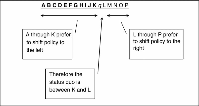
The approach to estimating policy locations is straightforward. The location of a policy status quo in ideological space can be estimated if we know legislators’ ideal points and the direction of change favored by each legislator on that policy issue. An analytical example illustrates this point. Imagine that there are 16 members of a legislature (A–P in Figure 2), with ideal points that line up perfectly on a single dimension. If each of these legislators reports whether he or she would support a slight shift in policy to the right or the left or prefer to maintain the same policy, then it is easy to identify the interval where the status quo is located. To the right of the status quo, legislators will prefer shifting policy to the right, and to the left of the status quo, they will prefer that it move to the left.Footnote ⁴ In the spatial model shown in Figure 2, members who prefer shifting the status quo to the left (A–K) are in boldface, and the status quo location can be identified. The status quo (q) is in the interval between K and L.

FIGURE 2.

Status Quo Location Identification Example

Legislator survey data to estimate status quo locations come from the National Political Awareness Test (NPAT) survey administered by Project Vote Smart (2008) in all congressional elections from 1994 through 2008.Footnote ⁵ Each survey includes a series of questions that use ordinal responses to evaluate candidates’ attitudes toward tax and spending issues. For each tax and spending question, responses were selected from among the following categories: eliminate, greatly decrease, slightly decrease, maintain status quo, slightly increase, and greatly increase. Question topics range widely, covering many areas of policy. For instance, I analyze questions involving spending on the arts, education, defense, intelligence, national parks, and welfare (among others) alongside tax questions covering capital gains, inheritance, gasoline, alcohol, cigarette, corporate, and personal income taxation, as well as earned income tax credit. The NPAT has the characteristics needed in a measure designed to estimate status quo locations. The ordinal measure in the NPAT has a maintain status quo response and multiple other responses that allow candidates to indicate the degree to which they want to increase or decrease a particular tax or spending policy. Furthermore, the responses members of Congress give on the NPAT align with their voting behavior. Ansolabehere, Snyder, and Stewart (Reference Ansolabehere, Snyder and Stewart2001a) calculate a single ideological dimension from the 1996 NPAT. Analysis of their data reveals that members’ NPAT responses correlate at 0.92 with First-Dimension DW NOMINATE scores for the 104th Congress. Although some close votes are likely subject to party pressure (Ansolabehere, Snyder, and Stewart Reference Ansolabehere, Snyder and Stewart2001b), the overall roll call voting record in Congress closely aligns with the preference information supplied by the NPAT.Footnote ⁶ The public context of the survey responses ensures that legislators will be motivated by nearly the same incentives that shape their votes.

To estimate status quo locations, the NPAT responses must be merged with a measure of legislator preferences, derived here from roll call votes. Legislators’ preferences are measured using the first dimension of Keith Poole's DW-NOMINATE common space scores (Poole Reference Poole2008). DW-NOMINATE common space scores provide an excellent overall summary of members’ preferences across a range of issues, for members of the House and Senate, along with the president. To check that the main dimension provides an adequate map of policy preferences across issues examined in this project, I estimated separate dimensions using W-NOMINATE for Defense, Foreign Policy/Foreign Aid, Tax and Budget, Energy and Environment, and Welfare and Human Services roll call votes, using issue codes supplied by Rohde (Reference Rohde2004) for the 105th House of Representatives. All dimensions correlated with the main NOMINATE dimension classified from all roll call votes at 0.92 or higher, with most correlated at above 0.97. With highly correlated preference orderings across issues, status quo locations estimated on the general dimension are close approximations of status quo locations estimated on issue-specific dimensions. Estimating status quo for multiple issues in a single common space facilitates statistical tests of theory predictions.Footnote ⁷

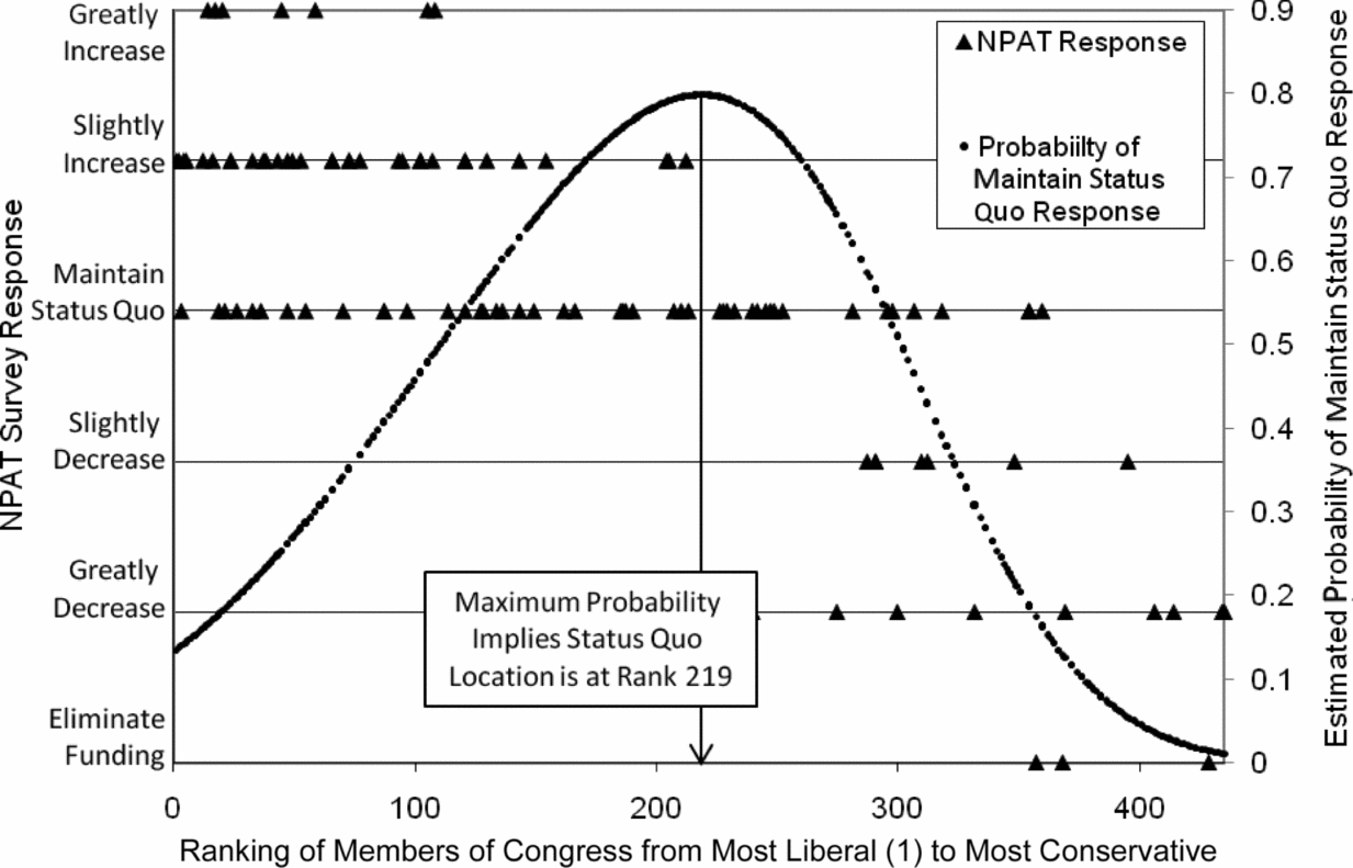
Figure 3 illustrates the result of merging roll call–derived preference locations with policy change preferences from the NPAT. On the x axis, members of the 109th House of Representatives are rank ordered from the most liberal at the far left to the most conservative at the far right (Poole Reference Poole2000). The y axis indicates legislators’ NPAT spending change preferences for the arts in 2006, ranging from some liberal members who wanted to greatly increase spending to a few conservative members near the far right side of the figure who wanted to entirely eliminate spending on the arts. The graph shows that as members became more conservative, support for government funding for the arts dropped, with a transition point near the middle of the graph from members favoring increases in spending to members favoring decreases. Representative Ramstad (rank 212) is the most conservative member to prefer an increase in spending, whereas Representative Emerson (rank 239.5) is the least conservative member to prefer a decrease. This suggests that the status quo was likely between rank 212 and rank 239.5.

FIGURE 3.

Estimated Status Quo Location for Spending on the Arts in 2006

I estimate status quo locations more precisely by using maximum likelihood estimation to identify the point that divides the ideological locations of legislators who prefer an increase above the status quo from those who prefer a decrease below the status quo. The particular approach involves using an ordered probit model to estimate survey responses on the basis of legislator preferences, and then calculating the probability of the “maintain status quo” response as a function of preferences.Footnote ⁸ In the example shown in Figure 3, the predicted probability of a maintain status quo response is superimposed on the survey responses. The rank with the highest predicted probability of responding with a preference for maintaining the status quo is rank 219, which suggests that the status quo is near this point. This estimate is, of course, necessarily somewhat imprecise. To characterize the uncertainty associated with particular estimated status quo, I construct bootstrapped standard errors by reestimating each status quo 1,000 times on samples drawn with replacement. The bootstrapped standard error of the status quo estimated in the figure is 13 ranks.

The estimated DW-NOMINATE status quo locations do a reasonable job of predicting NPAT spending preferences across a wide range of issues. Appendix B provides estimated status quo locations for 2008, along with bootstrapped standard errors and the proportion of NPAT responses (increase or decrease) correctly accounted for by the estimated status quo location. Appendix C provides information on the number of NPAT responses and issues, along with mean bootstrapped standard errors and mean percent predicted correctly by issue and year. Overall, 91% of NPAT increase or decrease responses are correctly explained by the estimated status quo location. All analyses that follow focus on issues where the DW-NOMINATE coefficient in the ordered probit model was statistically significant (p < .05, two tailed), with the estimated status quo within the (−1, 1) bounds of preferences in the DW-NOMINATE model. This excludes from consideration issues on which politics tends to be distributive rather than ideological, including agriculture policy, transportation policy, and (for most years) the NASA budget. Also excluded, because the NPAT survey does not include appropriate responses, are nonbudget and nontax issues (e.g., support for partial birth abortion).

A possible concern is that although Project Vote Smart claims to make an extensive effort to persuade candidates to complete its surveys, response rates are modest (see Appendix C for details). In addition, from the 106th Congress on, members of Congress with more conservative voting records (assessed using DW-NOMINATE first dimension) have responded less frequently to the NPAT than those with more liberal voting records. To test the estimates’ vulnerability to response bias and low response rates, I ran Monte Carlo simulations with low response rates and/or biased response rates. Neither random nonresponse nor nonresponse conditioned on ideology produced biased estimates, although lower response rates do decrease the precision of the estimates.Footnote ⁹

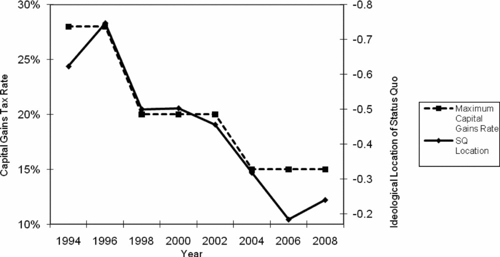
The resulting estimates change in ways that make sense. Figure 4 compares estimated status quo locations for capital gains taxes from 1994 to 2008 with the maximum capital gains tax rate. As shown, shifts in the estimated location of the status quo (right axis) closely parallel changes in the maximum capital gains tax rate. Because the tax rate was cut from 28% to 20%, and then cut again to 15%, the estimated status quo location became successively more conservative. Members of Congress responded to policy change by revising their preferences concerning future policy change, producing revised status quo location estimates.

FIGURE 4.

Capital Gains Tax Rates and Status Quo Locations

Source: Tax rate data from Citizens for Tax Justice (2011). “Top Federal Income Tax Rates since 1916,” www.ctj.org/pdf/regcg.pdf (accessed January 9, 2011).

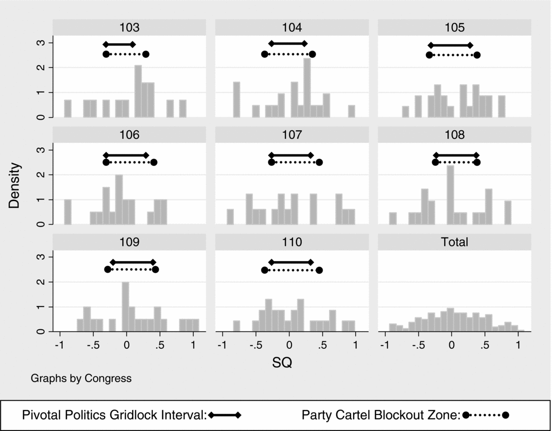
Figure 5 provides histograms of estimated status quo locations by session of Congress, with superimposed bars indicating the range of the pivotal politics gridlock interval and the party cartel blockout zone. The status quo locations charted in Figure 5 are the data analyzed in the remainder of the article. It is immediately clear that status quo are not tightly clustered at the center (e.g., at floor median)—that they are dispersed across a broad range of locations in each session of Congress. A substantial portion of these locations are within the pivotal politics gridlock interval, and an even larger portion falls within the party cartel blockout zone.Footnote ¹⁰

FIGURE 5.

Status Quo Location Histograms by Congress

STATUS QUO LOCATION TESTS

As discussed previously, each model predicts that status quo will be clustered in a particular gridlock interval or blockout zone. Table 1 reports the density of status quo in each hypothesized interval, along with the density in selected subintervals.

TABLE 1.

Status Quo Locations in 103rd through 110th Congresses: Consistent with Party Cartel or Pivotal Politics?

Notes: 167 status quo locations were assessed using (NPAT) survey at the end of each Congress, and gridlock/blockout zones were calculated using One-Dimensional DW-Nominate Common Space scores. Density is per 0.10 units of the ideological space.

The results reported in Table 1 indicate that both the pivotal politics and party cartel models are successful to a degree: they appropriately anticipate that issue status quos will tend to be clustered within the postulated gridlock interval or blockout zone.Footnote ¹¹ Nonetheless, the best-performing model is clearly the party cartel model. The density of status quo within the pivotal politics gridlock interval is 11 per 0.1 units of space, whereas the density in the party cartel blockout zone is 12.2. Conversely, the density of status quo is 7.1 outside the pivotal politics gridlock interval and only 5.8 outside the party cartel blockout zone. Because it is a model with partisan pivots, the party cartel blockout zone encompasses the pivotal politics gridlock interval, so these results reflect the fact that the region within the blockout zone but outside the gridlock interval contains a particularly dense concentration of status quo (14.8 per 0.1 units of ideological space). The distribution of status quo supports the party cartel model in another way as well. Because status quo outside the gridlock interval or blockout zone should be moved into the interval, we would expect to see a drop off in the density of status quo just outside the politically relevant interval. For the party cartel model, just such a drop off is observed. The density drops from 11.3 just inside the blockout zone to 9.7 just outside. For the pivotal politics model, however, the pattern is reversed: density increases from 8.0 just inside the gridlock interval to 12.7 just outside. These results suggest that parties matter in conjunction with pivotal politics as posited by the party cartel model: minority party pivots seem to be subject to partisan pressure and the majority party appears to be able to block policy change.

RATE OF POLICY CHANGE TESTS

Central to the concept of the gridlock interval or blockout zone is the idea that policies within this interval will be more difficult to change because pivotal actors or party leaders disagree about the appropriate direction for policy change. Issues with status quo that begin a session of Congress within the gridlock interval or blockout zone are expected to experience less change by the end of the session than issues that were initially outside the interval because any major legislative change is likely to be vetoed, filibustered, or blocked.Footnote ¹²

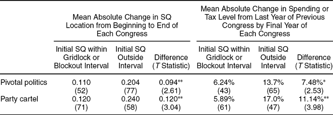
I use two measures of policy change to test this expectation. The first measure evaluates changes in estimated status quo locations—the difference between an issue's status quo location at the beginning and end of a session of Congress measures how much members of Congress perceived that a particular status quo changed. The analysis of status quo changes includes 129 observations. A problem with this measure is that extreme status quos are often measured with less precision because there are fewer members in this region of ideological space; thus, these issues will tend to change more simply because they are subject to more measurement error. I address this problem in two ways: by weighting the mean so status quo that are measured more precisely receive more weight, and by including a second change measure that does not suffer from this measurement error. The mean values reported in Table 2 are weighted using an analytic weight based on the inverse of the bootstrapped standard error of the status quo.Footnote ¹³ The second change measure assesses the degree to which the underlying policy (tax rate or spending level) did in fact change. For each issue, I attempted to identify a measure of the actual budgeted spending level (Office of Management and Budget 2010; True Reference True2009) or the actual tax rate. Unfortunately, it was not possible to make this match for every issue. For example, CIA appropriations (an issue measured by the NPAT for several years) are not publically available and spending on AIDS research does not constitute a separate budget subfunction, so this analysis includes only 108 observations. I measure changes in spending and taxes by contrasting the spending or tax level in the last budget year fully under the control of one Congress (e.g., the 2010 budget for the 111th Congress) with the spending or tax level at the same point in the previous Congress.Footnote ¹⁴

TABLE 2.

Rate of Status Quo Change in 103rd through 110th Congresses: Consistent with Party Cartel or Pivotal Politics?

Notes: Number of issue status quo in each group is in parentheses. Mean SQ spending change measures are weighted by the bootstrapped standard error of the status quo estimate.

*p < .01; **p < .005 (one tailed).

Table 2 reports on tests that evaluate whether status quo change less when they are within the gridlock interval or blockout zone. The results provide some support for both models, although the party cartel model once again appears to outperform the pivotal politics model.Footnote ¹⁵ Issues outside the pivotal politics gridlock interval changed on average by 0.94 points more than issues within the gridlock interval (p < .005), whereas issues outside the party cartel blockout zone changed 0.12 points more than issues within the blockout zone (p < .005). These results are corroborated by the analysis of real tax and spending changes. Issues outside the gridlock interval changed on average by 7.48% more than those inside the interval (p < .01), whereas issues outside the party cartel blockout zone changed by 11.14% more than those inside the blockout zone (p < .0001). Overall, the pivotal politics model performs well, but the party cartel model outperforms it. Apparently, parties matter in combination with pivotal politics as posited by my adaptation of the party cartel model.

PREDICTING POLICY CHANGE

The panel data analysis reported here models change over time in status quo locations as predicted by each theory. This provides the sharpest and most precise test of the theories’ predictions. For each Congress, the status quo for each issue starts out at some initial location (q_it−1), and each theory provides a prediction concerning how this initial location will be shifted to a new final location (q_it). The main independent variables in the analysis are the predicted final status quo locations from each model as described previously and in Equations (1) through (4) of Appendix A. In the analyses reported here, each observation is transformed to adjust for the heteroscedastic errors implied by variation in the precision with which particular status quo are estimated (Hardin Reference Hardin1997).

In addition to policy action, inflation may be expected to alter the locations of particular status quo. If gridlocked or blocked issues cannot be changed through positive action, then they might nonetheless be adjusted through inaction in the face of inflation. Issues where inflation-diminished spending or inflation-altered tax receipts should lead policy to drift toward policies preferred by conservatives are coded 1 (e.g., education, gasoline taxes, and the environment). Issues where inflation should lead policy or tax rates to drift away from policies supported by conservatives are coded −1 (e.g., defense spending and the child tax credit). Issues where inflation should not matter are coded 0 (e.g., the inflation-adjusted earned income tax credit). Given the coding, the inflation parameter should have a positive sign. Inflation should principally influence status quo location when issues are initially within the gridlock interval or blockout zone because policy makers will have less opportunity to address the consequences of inflation. Therefore, the inflation drift parameter is nonzero only when the initial status quo location is in the relevant gridlock interval or blockout zone.Footnote ¹⁶

The model to be estimated is:

In the model, q_it is the status quo for issue i in Congress t, prediction_it is the predicted location of the status quo for issue i in Congress t as derived from each model so its coefficient is expected to equal 1, and inflation_it reflects the direction inflation is expected to move the status quo of issue i during periods when its status quo is gridlocked or blocked. Because theory implies that the intercept should be zero, I do not include a constant term in the models.Footnote ¹⁷

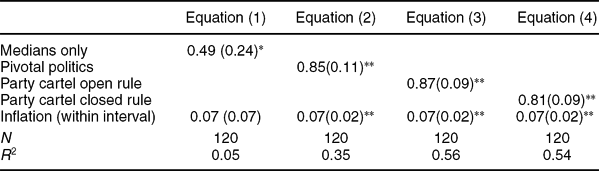
Table 3 reports the results of a linear regression model with panel corrected standard errors.Footnote ¹⁸ The dependent variable is the status quo estimate at the end of a session of Congress. Equations (1) through (4) test each model separately. The key independent variable in each equation is the predicted final status quo location derived from that model. Predicted locations are regressed on actual final locations while controlling for the effect of inflation within the gridlock interval or blockout zone.

TABLE 3.

Modeling Status Quo Locations and Policy Changes in 103rd through 110th Congresses

Note: Linear regression model with panel corrected standard errors.

*p < .05; **p < .001 (two tailed).

The simple median model proves to be the weakest. Although the median model coefficient is statistically significant in Table 3 (p < .05), the R ² of only 0.05 suggests that it accounts for a relatively small portion of the variance in status quo locations. Although simple, this model is apparently too simple to explain status quo locations with much accuracy.

The predictions of the pivotal politics model are substantially more accurate [Equation (2)]. The pivotal politics location prediction is statistically significant (p < .001) with the expected sign. The associated R ² is 0.35. Thus, adding pivotal politics dramatically improves on the predictions that can be made using the median model. The estimated coefficient of 0.85 is not statistically distinguishable from the theoretically expected value of 1. Clearly, pivotal politics outperforms the median model.

Adding parties further improves predictive accuracy. The open rule party cartel model [Equation (3)] substantially outperforms the pivotal politics model. The prediction is statistically significant (p < .001), with an associated R ² of 0.56 that reflects a substantially better fit than the pivotal politics model. The estimated coefficient (0.87) is also not statistically distinguishable from the theoretically expected value of 1. This result is consistent with my assumption that both the majority and minority parties exert influence in the U.S. Congress by pressuring pivotal party members to uphold Cox and McCubbins’ “first commandment” to not support legislation opposed by a majority of their party.Footnote ¹⁹

The closed rule party cartel model assumes that parties exert substantially more influence. In particular, the majority party can use positive agenda power to “pull” outcomes toward the majority party medians. The closed rule party cartel model performs slightly worse than the open rule model, but the difference in fit between the models is modest enough that no definitive conclusions can be drawn. The estimated coefficient is statistically significant (p < .001), but it is slightly smaller than the coefficient for the open rule model (and it is significantly different from the theoretically expected value of 1, which suggests that status quo locations do not change as much as the closed rule model predicts). The R ² of 0.54 is marginally smaller than that for the open rule model. Thus, although there is substantial evidence that parties engage in blocking (negative agenda control), assuming that they engage in positive agenda control as well does not appear to improve (or greatly degrade) predictive accuracy. Perhaps this reflects a mix of open rule and closed rule influences. Although the House majority uses closed rules to exercise positive agenda control, the Senate majority has far fewer powers. Once in conference, House negotiators will consider alternatives that were ruled out by their closed rule. Even for the House of Representatives, Cox and McCubbins (Reference Cox and McCubbins2005) argue that negative agenda power (e.g., blocking under open rule) is a constant source of party influence, whereas parties only exercise substantial positive agenda control in some circumstances.

In each equation, the inflation parameter performs as expected. Inflation shifts status quo in a conservative direction when it reduces effective spending on liberal priorities (e.g., education spending) and conversely inflation moves conservative priorities in a liberal direction (e.g., defense spending). Across analyses inflation has a consistent effect, shifting status quo by roughly 0.07 points on the ideological dimension. Inflation appears to have substantial policy consequences for gridlocked issues.