3.1. Spectral POD

The frequency domain form of the proper orthogonal decomposition (POD), referred to as SPOD, is an orthonormal basis of modes that (i) oscillate at a given frequency, (ii) are perfectly coherent and (iii) are decorrelated from each other. It constitutes a procedure to extract coherent structures from data evolving at a given frequency. A complete description is performed in Towne et al. (Reference Towne, Schmidt and Colonius2018). Spectral POD modes are eigenfunctions of the CSD tensor ${\boldsymbol{\mathsf{S}}}$, obtained as

(3.1) \begin{align} {\boldsymbol{\mathsf{S}}}(\alpha,y,y',\beta,\omega)&=\frac{1}{L_xL_z}\int_{-\infty}^{\infty} \int_{0}^{L_x}\int_{0}^{L_z}{\boldsymbol{\mathsf{C}}}(x-x',y,y', \nonumber\\ &\quad z-z',\tau)\ \textrm{e}^{\textrm{i}(\omega \tau-\alpha (x-x')-\beta (z-z'))}\,\mathrm{d}\tau\,\mathrm{d} (x-x') \,\mathrm{d} (z-z') , \end{align}

where ${\boldsymbol{\mathsf{C}}}(x-x',y,y',z-z',t-t')$ is the two-point space–time correlation tensor. Homogeneity in $x$, $z$ and $t$ allows us to express the dependence in each direction using Fourier modes, as shown in (3.1). Thus, for each $(\alpha , \beta ,\omega )$ combination, the eigendecomposition

(3.2)\begin{equation} \int_{{-}1}^1 {\boldsymbol{\mathsf{S}}}(y,y')\boldsymbol{\phi}_j(y') \,\mathrm{d} y=\lambda_j \boldsymbol{\phi}_j(y) \end{equation}

leads to an orthonormal basis of SPOD modes (since ${\boldsymbol{\mathsf{S}}}(y,y')$ is Hermitian), with respect to the inner product $(a(y),b(y))_y=\int _{-1}^1 a(y)b(y)\,\mathrm {d} y$. The real eigenvalues $\lambda _j$ represent the relative contribution of a given mode to the CSD.

In practice, SPOD modes are computed by splitting the signal into an ensemble of $M$ possibly overlapping time windows of size $N$, whose snapshots $\boldsymbol {u}_i^{(n)}$ are spaced ${\rm \Delta} t$ apart,

(3.3)\begin{equation} {\boldsymbol{\mathsf{U}}}^{(n)}=[\boldsymbol{u}_1^{(n)},\ldots,\boldsymbol{u}_N^{(n)}], \end{equation}

where $n$ is the index related to the data block. A discrete Fourier transform is performed on each block,

(3.4)\begin{equation} \hat{{\boldsymbol{\mathsf{U}}}}^{(n)}=[\hat{\boldsymbol{u}}_{\omega_1}^{(n)},\ldots, \hat{\boldsymbol{u}}_{\omega_N}^{(n)}], \end{equation}

with

(3.5)\begin{equation} \hat{\boldsymbol{u}}_{\omega_k}^{(n)}=\sum_{j=1}^{N}w_j\boldsymbol{u}_j^{(n)}\textrm{e}^{\textrm{i} 2{\rm \pi} (k-1)(j-1)/N}\,{\rm \Delta} t, \end{equation}

and $w_j$ are weights of a window function designed to reduce effects of non-periodicity of the signal in the data block. The window is normalised such that $\sum _{i=1}^{N}w_i^2=1$ to be consistent with the energy contained in the signal. Then, a POD is performed onto the ensemble of Fourier components at a given frequency such that

(3.6)\begin{equation} \tilde{{\boldsymbol{\mathsf{S}}}}_{\omega_k}{\boldsymbol{\mathsf{W}}}\boldsymbol{\varPhi}_{j, \omega_k}^{\textit{SPOD}}=\lambda_{j,\omega_k}\boldsymbol{\varPhi}^{\textit{SPOD}}_{j,\omega_k}, \end{equation}

with the estimate of the CSD matrix

(3.7)\begin{equation} \tilde{{\boldsymbol{\mathsf{S}}}}_{\omega_k}=\frac{1}{{\rm \Delta} t M} \sum_{n=1}^{M}\hat{\boldsymbol{u}}_{\omega_k}^{(n)}(\hat{\boldsymbol{u}}_{\omega_k}^{(n)})^*, \end{equation}

and ${\boldsymbol{\mathsf{W}}}$ a matrix of weights defining the spatial inner product $(\boldsymbol {a},\boldsymbol {b})_{W}=\boldsymbol {a}^*{\boldsymbol{\mathsf{W}}}\boldsymbol {b}$, numerical approximation of $(a(y),b(y))_y$, with $\boldsymbol {\cdot }^*$ denoting the transpose-conjugate operation. Functions $\boldsymbol {\varPhi }^{\textit{SPOD}}_{j,\omega _k}$ are the SPOD modes and $\lambda _{j,\omega _k}$ are the associated eigenvalues.

In our numerical tests, we use $N=256$ (respectively $N=512$) at $Re_\tau =180$ (respectively $Re_\tau =550$) with an overlap of $\frac {3}{4}N$ and $w_j=2\sin ^2({\rm \pi} (j-1)/N))$.

We can see that SPOD modes are principal components of an ensemble of solutions defined in the Fourier domain. This random variability between ensemble members $\hat {\boldsymbol {u}}_{\omega }^{(n)}$ of the same statistically stationary flow reflects the effect of turbulence on waves, which cannot be properly represented by a single deterministic Fourier mode. Indeed, a deterministic purely coherent wave not affected by the turbulence would result in identical values of $\hat {\boldsymbol {u}}_{\omega }^{(n)}$ and then in a single SPOD mode equal to the Fourier coefficient. We will see that the stochastic linear problem presented in § 4.2 shares common structures with the SPOD that makes them consistent and comparable.

3.2. Resolvent analysis

Resolvent analysis aims at exploring the response of a linearised system to external forcing, interpreted as unknown nonlinearities when analysing turbulent flows (Hwang & Cossu Reference Hwang and Cossu2010; McKeon & Sharma Reference McKeon and Sharma2010). We start with the incompressible Navier–Stokes equations

(3.8)\begin{equation} \left. \begin{array}{c@{}} \displaystyle \displaystyle \dfrac{\partial{\boldsymbol{u}}}{\displaystyle \partial{t}}+(\boldsymbol{u}\boldsymbol{\cdot} \boldsymbol{\nabla})\boldsymbol{u}={-}\boldsymbol{\nabla} p + \dfrac{1}{Re}{\rm \Delta}\boldsymbol{u},\\ \boldsymbol{\nabla}\boldsymbol{\cdot} \boldsymbol{u}=0. \end{array} \right\} \end{equation}

Expressing (3.8) in the Fourier domain and splitting the solution into the parallel mean flow $U(y)$ and fluctuations $\boldsymbol {u}'$ leads to the system

(3.9)\begin{equation} { \begin{pmatrix} A(\boldsymbol{\cdot})+D(\boldsymbol{\cdot}) & \displaystyle \frac{\partial{U}}{\displaystyle \partial{y}} & 0 & i\alpha \\ 0 & A(\boldsymbol{\cdot})+D(\boldsymbol{\cdot}) & 0 & \displaystyle \frac{\partial{\boldsymbol{\cdot}}}{\displaystyle \partial{y}} \\ 0 & 0 & A(\boldsymbol{\cdot})+D(\boldsymbol{\cdot}) & i\beta \\ i\alpha & \displaystyle \frac{\partial{\boldsymbol{\cdot}}}{\displaystyle \partial{y}} & i\beta & 0 \\ \end{pmatrix} \begin{pmatrix} \hat{u}_{\alpha,\beta,\omega}\\ \hat{v}_{\alpha,\beta,\omega}\\ \hat{w}_{\alpha,\beta,\omega}\\ \hat{p}_{\alpha,\beta,\omega}\\ \end{pmatrix} = \begin{pmatrix} \hat{f}_x\\ \hat{f}_y\\ \hat{f}_z\\ 0 \end{pmatrix} } , \end{equation}

with the advection operator $A(\boldsymbol {\cdot })=-i\omega +i\alpha U$, the diffusion operator $D(\boldsymbol {\cdot })=-({1}/{Re})(-\alpha ^2 + \partial ^{2}\boldsymbol {\cdot } / \partial y^{2} -\beta ^2)$, $Re$ the Reynolds number and

(3.10) \begin{equation} \left.\begin{array}{c@{}} \hat{f}_x={\boldsymbol{\mathsf{F}}}_{\alpha,\beta,\omega}(\overline{\boldsymbol{u}' \boldsymbol{\cdot} \boldsymbol{\nabla} u'}-{\boldsymbol{u}' \boldsymbol{\cdot} \boldsymbol{\nabla} u'}),\\ \hat{f}_y={\boldsymbol{\mathsf{F}}}_{\alpha,\beta,\omega}(\overline{\boldsymbol{u}' \boldsymbol{\cdot} \boldsymbol{\nabla} v'}-{\boldsymbol{u}' \boldsymbol{\cdot} \boldsymbol{\nabla} v'}),\\ \hat{f}_z={\boldsymbol{\mathsf{F}}}_{\alpha,\beta,\omega}(\overline{\boldsymbol{u}' \boldsymbol{\cdot} \boldsymbol{\nabla} w'}-{\boldsymbol{u}' \boldsymbol{\cdot} \boldsymbol{\nabla} w'}), \end{array}\right\} \end{equation}

where ${\boldsymbol{\mathsf{F}}}_{\alpha ,\beta ,\omega }(\boldsymbol {\cdot })$ denotes the space–time Fourier transform.

Equation (3.9) can be written more compactly as

(3.11)\begin{equation} ({\boldsymbol{\mathsf{A}}}_{\alpha,\beta,\omega}-i\omega{\boldsymbol{\mathsf{E}}}) \hat{\boldsymbol{q}}_{\alpha,\beta,\omega}={\boldsymbol{\mathsf{L}}}_{\alpha,\beta, \omega}\hat{\boldsymbol{q}}_{\alpha,\beta,\omega}={{\boldsymbol{\mathsf{N}}}_{\alpha, \beta,\omega}(\boldsymbol{u}')}, \end{equation}

where ${\boldsymbol{\mathsf{A}}}_{\alpha ,\beta ,\omega }$ is the linearised Navier–Stokes operator under the considered assumptions and ${\boldsymbol{\mathsf{E}}}$ is a diagonal matrix with $1$ and $0$ values for velocity and pressure components, respectively. Here ${\boldsymbol{\mathsf{L}}}_{\alpha ,\beta ,\omega }^{-1}=({\boldsymbol{\mathsf{A}}}_{\alpha , \beta ,\omega }-i\omega {\boldsymbol{\mathsf{E}}})^{-1}$ is the resolvent of the operator ${\boldsymbol{\mathsf{A}}}_{\alpha ,\beta ,\omega }$. Formally, the nonlinear term ${\boldsymbol{\mathsf{N}}}_{\alpha ,\beta ,\omega }(\boldsymbol {u}')$ can be considered as a right-hand side of (3.11). However, the Fourier transform of a product is a convolution, which results in an integral over all frequency-wavenumbers (Cavalieri et al. Reference Cavalieri, Jordan and Lesshafft2019; McKeon & Sharma Reference McKeon and Sharma2010), which is incompatible with a prediction for an ‘isolated’ frequency-wavenumber combination; the nonlinear term couples the various frequencies and wavenumbers in the Navier–Stokes system in triadic interactions. The goal of resolvent analysis is to explore the response of the linear operator ${\boldsymbol{\mathsf{L}}}_{\alpha ,\beta ,\omega }$ to nonlinearities treated as an external forcing. In what follows we will consider the discretised form of (3.11), which, with the addition of an external forcing, becomes

(3.12)\begin{equation} {\boldsymbol{\mathsf{L}}}_{\alpha,\beta,\omega}\hat{\boldsymbol{q}}_{\alpha,\beta, \omega}={{\boldsymbol{\mathsf{B}}}}\hat{\boldsymbol{f}}_{\alpha,\beta,\omega}. \end{equation}

Since nonlinear terms act only on the momentum equations in (3.9), and since SPOD modes can be calculated separately once the velocity is known, we define input and output matrices respectively as

(3.13a,b)\begin{equation} {\boldsymbol{\mathsf{B}}}=\begin{pmatrix} \mathbb{I} & 0 & 0\\ 0 & \mathbb{I} & 0\\ 0 & 0 & \mathbb{I}\\ 0 & 0 & 0 \end{pmatrix} \quad \text{and} \quad {\boldsymbol{\mathsf{H}}}=\begin{pmatrix} \mathbb{I} & 0 & 0 & 0 \\ 0 & \mathbb{I} & 0 & 0 \\ 0 & 0 & \mathbb{I} & 0 \end{pmatrix} . \end{equation}

The output matrix ${\boldsymbol{\mathsf{H}}}$ thus extracts only the velocity components, which may be combined in an inner product whose norm is the kinetic energy. The response to a harmonic forcing $\hat {\boldsymbol {f}}_{\alpha ,\beta ,\omega }$ is ${\boldsymbol{\mathsf{H}}}\hat {\boldsymbol {q}}_{\alpha ,\beta ,\omega }={\boldsymbol{\mathsf{H}}} {\boldsymbol{\mathsf{L}}}_{\alpha ,\beta ,\omega }^{-1}{\boldsymbol{\mathsf{B}}}\hat {\boldsymbol {f}}_{\alpha ,\beta ,\omega }$. The frequency response operator is thus defined from the resolvent operator, ${\boldsymbol{\mathsf{L}}}_{\alpha ,\beta ,\omega }^{-1}$, as ${\boldsymbol{\mathsf{R}}}_{\alpha ,\beta ,\omega }={\boldsymbol{\mathsf{H}}}{\boldsymbol{\mathsf{L}}}_{\alpha , \beta ,\omega }^{-1}{\boldsymbol{\mathsf{B}}}$. We then search for the forcing that maximises

(3.14)\begin{equation} \max_{\hat{\boldsymbol{f}}_{\alpha,\beta,\omega}}\frac{\|{\boldsymbol{\mathsf{H}}} \hat{\boldsymbol{q}}_{\alpha,\beta,\omega}\|^2_W}{\|\hat{\boldsymbol{f}}_{\alpha,\beta,\omega}\|^2_W} =\frac{\|{\boldsymbol{\mathsf{R}}}_{\alpha,\beta,\omega}\hat{\boldsymbol{f}}_{\alpha,\beta, \omega}\|^2_W}{\|\hat{\boldsymbol{f}}_{\alpha,\beta,\omega}\|^2_W}.\end{equation}

The maximisation of the Rayleigh quotient (3.14) can be achieved by means of the following singular value decomposition:

(3.15)\begin{equation} {\boldsymbol{\mathsf{W}}}^{1/2}{\boldsymbol{\mathsf{R}}}_{\alpha,\beta,\omega}{\boldsymbol{\mathsf{W}}}^{{-}1/2} ={\boldsymbol{\mathsf{U}}}_r\boldsymbol{\varSigma}_r {\boldsymbol{\mathsf{V}}}_r^*. \end{equation}

Here ${\boldsymbol{\mathsf{W}}}^{1/2}$ is defined by the Cholesky decomposition ${\boldsymbol{\mathsf{W}}}={\boldsymbol{\mathsf{W}}}^{1/2}({\boldsymbol{\mathsf{W}}}^{1/2})^*$ with ${\boldsymbol{\mathsf{W}}}$ defined in § 3.1, ${{\boldsymbol{\mathsf{U}}}_r=(\boldsymbol {U}_{r,1},\ldots ,\boldsymbol {U}_{r,N})}$ and ${{\boldsymbol{\mathsf{V}}}_r=(\boldsymbol {V}_{r,1},\ldots ,\boldsymbol {V}_{r,N})}$ are orthonormal matrices and ${\boldsymbol {\varSigma }_r}= diag(s_1,\ldots ,s_N)$ is a diagonal matrix. We define the optimal forcing modes as $\boldsymbol {\varPsi }^{\textit{resolvent}}_i={\boldsymbol{\mathsf{W}}}^{-1/2}{\boldsymbol {V}_{r,i}}$ and the associated optimal response modes (also referred to as resolvent modes in the following) as $\boldsymbol {\varPhi }_i^{\textit{resolvent}}={\boldsymbol{\mathsf{W}}}^{-1/2}{\boldsymbol {U}_{r,i}}$. The singular values, $s_i$, diagonal elements of ${\boldsymbol {\varSigma }_r}$ sorted in descending order, indicate the gains associated with forcing-response mode pairs.

As shown in Towne et al. (Reference Towne, Schmidt and Colonius2018), resolvent modes and SPOD correspond if and only if the forcing in the data correspond to a Gaussian white noise. However, if there is a separation in gain between the optimal forcing-response pair and suboptimal ones, even coloured forcing leads to a dominance of the optimal response in the flow CSD, unless the forcing is strongly biased towards suboptimals (Beneddine et al. Reference Beneddine, Sipp, Arnault, Dandois and Lesshafft2016; Cavalieri et al. Reference Cavalieri, Jordan and Lesshafft2019). A way to account for a part of this forcing is to consider a triple decomposition of the velocity field in the line of the work of Reynolds & Tiederman (Reference Reynolds and Tiederman1967) and Reynolds & Hussain (Reference Reynolds and Hussain1972) where the Reynolds stresses induced by the incoherent part of the turbulent velocity through ensemble averaging is modelled by an eddy viscosity in the linearised operator, noted ${\boldsymbol{\mathsf{L}}}_{\alpha ,\beta ,\omega }^{\nu _t}$. It corresponds to a modification of the system (3.8), where the diffusion operator $({1}/{Re}){\rm \Delta} \boldsymbol {u}$ is replaced by $\boldsymbol {\nabla }\boldsymbol {\cdot }(({1}/{Re}+\nu _t(y))(\boldsymbol {\nabla }\boldsymbol {u}+\boldsymbol {\nabla }\boldsymbol {u}^\textrm {T}))$, leading to the system

(3.16)\begin{equation} \begin{pmatrix} A(\boldsymbol{\cdot})+D_{\nu_t}(\boldsymbol{\cdot}) & \displaystyle \frac{\partial{U}}{\displaystyle \partial{y}}-i\alpha\displaystyle \frac{\partial{\nu}}{\displaystyle \partial{y}} & 0 & i\alpha \\ 0 & A(\boldsymbol{\cdot})+D_{\nu_t}(\boldsymbol{\cdot})-\displaystyle \frac{\partial{\nu}}{\displaystyle \partial{y}} \displaystyle \frac{\partial{\boldsymbol{\cdot}}}{\displaystyle \partial{y}} & 0 & \displaystyle \frac{\partial{\boldsymbol{\cdot}}}{\displaystyle \partial{y}} \\ 0 & -i\beta\displaystyle \frac{\partial{\nu}}{\displaystyle \partial{y}} & A(\boldsymbol{\cdot})+D_{\nu_t}(\boldsymbol{\cdot}) & i\beta \\ i\alpha & \displaystyle \frac{\partial{\boldsymbol{\cdot}}}{\displaystyle \partial{y}} & i\beta & 0 \\ \end{pmatrix} \begin{pmatrix} \hat{u}_{\alpha,\beta,\omega}\\ \hat{v}_{\alpha,\beta,\omega}\\ \hat{w}_{\alpha,\beta,\omega}\\ \hat{p}_{\alpha,\beta,\omega}\\ \end{pmatrix} = \begin{pmatrix} \hat{f}_x \\ \hat{f}_y \\ \hat{f}_z \\ 0 \end{pmatrix},\end{equation}

with

(3.17)\begin{equation} D_{\nu_t}(\boldsymbol{\cdot})={-}\left(\frac{1}{Re}+\nu_t\right)\left(-\alpha^2 + \displaystyle \frac{\partial^{2}{\boldsymbol{\cdot}}}{\displaystyle \partial{y}^{2}} -\beta^2 \right)-\displaystyle \frac{\partial{\nu_t}}{\displaystyle \partial{y}} \displaystyle \frac{\partial{\boldsymbol{\cdot}}}{\displaystyle \partial{y}}. \end{equation}

In this work we choose to fix the turbulent viscosity parameter, $\nu _t$, with the Cess's model (Cess Reference Cess1958) as in Del Álamo & Jiménez (Reference Del Álamo and Jiménez2006) and Pujals et al. (Reference Pujals, García-Villalba, Cossu and Depardon2009), i.e.

(3.18)\begin{equation} { \nu_t=\frac{1}{Re}\left(\frac{1}{2}\left(1+\frac{\kappa^2Re_\tau^2}{9}(1 -y^2)^2(1+2y^2)^2(1-e^{-\frac{y^+}{A}})^2\right)^{1/2}-\frac{1}{2}\right), } \end{equation}

where $y^+=Re_\tau (1-|y|)$, $\kappa =0.426$ is the von Kármán constant and $A=25.5$ is a constant chosen consistently following Pujals et al. (Reference Pujals, García-Villalba, Cossu and Depardon2009). The corresponding resolvent analysis will be referred to as eddy-viscosity resolvent analysis. For compactness and to avoid confusions, standard resolvent analysis will be noted $\nu$-resolvent and eddy-viscosity resolvent will be noted $\nu _t$-resolvent. Recent results have shown that the inclusion of an eddy viscosity in the linearised operator improves the agreement between resolvent modes and simulation data (Illingworth, Monty & Marusic Reference Illingworth, Monty and Marusic2018; Morra et al. Reference Morra, Semeraro, Henningson and Cossu2019), as the eddy-viscosity models part of the forcing statistics (Morra et al. Reference Morra, Nogueira, Cavalieri and Henningson2021).

In any case, the resolvent modes constitute a basis where any forcing can be projected onto the forcing modes and, thus, we can deduce the response to this forcing. Extracting statistics of the nonlinear term is a hard task in itself, and examples are shown by Zare et al. (Reference Zare, Jovanović and Georgiou2017), Nogueira et al. (Reference Nogueira, Morra, Martini, Cavalieri and Henningson2021), Towne et al. (Reference Towne, Lozano-Durán and Yang2020) and Morra et al. (Reference Morra, Nogueira, Cavalieri and Henningson2021), where DNS data was used for that matter. To avoid the need of detailed data for predictions, some modelling of the unknown forcing is necessary. We propose in this paper to extend such an analysis to a framework introducing a statistical modelling of the fluctuating velocities and a stochastic transport equation, with modelling of unresolved velocity as a Brownian motion. This is described next.

4.1. Stochastic Navier–Stokes equations under location uncertainty

The starting point of our modelling approach is the stochastic model proposed by Mémin (Reference Mémin2014). It relies on the decomposition of the Lagrangian transport of a particle by a resolved velocity $\boldsymbol {u}$ perturbed by a function of a Brownian motion $\boldsymbol {B}_t$, written as a stochastic Itô process. The displacement $\boldsymbol {X}(\boldsymbol {x},t)$ of a particle from time $t_0$ to $t$ is thus written as

(4.1)\begin{equation} \boldsymbol{X}(\boldsymbol{x},t)=\boldsymbol{X}(\boldsymbol{x},t_0)+\int_{t_0}^t\boldsymbol{u}(\boldsymbol{x},t) \,\mathrm{d}t+\int_{t_0}^t\boldsymbol{\sigma} \,\mathrm{d}\boldsymbol{B}_t, \end{equation}

or in a more usual and compact differential form as

(4.2)\begin{equation} \mathrm{d}\boldsymbol{X}(\boldsymbol{x},t)=\boldsymbol{u}(\boldsymbol{x},t)\,\mathrm{d}t +\boldsymbol{\sigma} \,\mathrm{d}\boldsymbol{B}_t. \end{equation}

The term $\boldsymbol {\sigma } \,\mathrm {d}\boldsymbol {B}_t$ hides a spatial convolution in the domain $\varOmega$ between the modelled bounded deterministic correlation kernel $\boldsymbol {\sigma }(\boldsymbol {x},\boldsymbol {x}',t)$ and $\,\mathrm {d}\boldsymbol {B}_t$ the increment of the Brownian motion $\boldsymbol {B}_t$ (i.e. $\,\mathrm {d}\boldsymbol {B}_t=\boldsymbol {B}_{t+\mathrm {d} t}-\boldsymbol {B}_t$) such that its $i$th component at the spatial location $\boldsymbol {x}$ is given by the following kernel integral expression:

(4.3)\begin{equation} (\boldsymbol{\sigma} \,\mathrm{d}\boldsymbol{B}_t)_{\boldsymbol{x}}^i= \int_\varOmega\boldsymbol{\sigma}^{ij}(\boldsymbol{x},\boldsymbol{x}',t)\,\mathrm{d} \boldsymbol{B}_t^j(\boldsymbol{x}')\,\mathrm{d}\boldsymbol{x}'. \end{equation}

This formulation models the transport of physical quantities by a smooth resolved velocity (i.e. differentiable in time), perturbed by a noise that is assumed to be correlated and smooth in space (through the correlation kernel $\boldsymbol {\sigma }$) but decorrelated and non-differentiable in time. This ground assumption in Itô calculus is as well classically performed in standard stochastic forcing models, and is relaxed in Zare et al. (Reference Zare, Jovanović and Georgiou2017) for a time-domain formulation. The strong hypothesis of time-decorrelated multiplicative noise is clearly a limitation of the proposed formalism. However, introducing a time memory would require considering high-order terms in the stochastic Taylor expansions in Itô calculus (Kloeden & Platen Reference Kloeden and Platen2013) and is beyond the scope of the present paper.

The statistical behaviour of the noise is an information that has to be specified. The operator $\boldsymbol {\sigma }$ is built in order to respect the given covariance tensor of the unresolved part

(4.4)\begin{align} \mathbb{E}((\boldsymbol{\sigma} \,\mathrm{d}\boldsymbol{B}_t)_{\boldsymbol{x}}^i(\boldsymbol{\sigma} \,\mathrm{d}\boldsymbol{B}_{t'})_{\boldsymbol{x}'}^j) &=\int_\varOmega \int_\varOmega \boldsymbol{\sigma}^{ik}(\boldsymbol{x},\boldsymbol{y},t)\mathbb{E}(\mathrm{d}\boldsymbol{B}_t^k (\boldsymbol{y})\,\mathrm{d}\boldsymbol{B}_{t'}^l(\boldsymbol{y}')) \boldsymbol{\sigma}^{lj}(\boldsymbol{x}',\boldsymbol{y}',t')\,\mathrm{d}\boldsymbol{y}\,\mathrm{d}\boldsymbol{y}' \nonumber\\ &=\int_\varOmega \int_\varOmega \boldsymbol{\sigma}^{ik}(\boldsymbol{x},\boldsymbol{y},t)(\delta(\boldsymbol{y}- \boldsymbol{y}')\delta(t-t')\delta_{kl})\,\mathrm{d} t\,\boldsymbol{\sigma}^{lj}(\boldsymbol{x}',\boldsymbol{y}',t')\, \mathrm{d}\boldsymbol{y}\,\mathrm{d}\boldsymbol{y}' \nonumber\\ &=\int_\varOmega\boldsymbol{\sigma}^{ik}(\boldsymbol{x},\boldsymbol{y},t) \boldsymbol{\sigma}^{kj}(\boldsymbol{x}',\boldsymbol{y},t')\,\mathrm{d}\boldsymbol{y}\,\delta(t-t')\,\mathrm{d} t \nonumber\\ &\overset{!}{=}{\boldsymbol{\mathsf{Q}}}(\boldsymbol{x},\boldsymbol{x}',t)\,\delta(t-t')\,\mathrm{d} t, \end{align}

with $\,\mathrm {d}\boldsymbol {B}_t^i$ the $i$th component of $\,\mathrm {d}\boldsymbol {B}_t$ and $\mathbb {E}$ the expectation operator. We define as well the variance tensor

(4.5)\begin{equation} {\boldsymbol{\mathsf{a}}}(\boldsymbol{x},t)={\boldsymbol{\mathsf{Q}}}(\boldsymbol{x},\boldsymbol{x},t). \end{equation}

We can remark that the tensor ${\boldsymbol{\mathsf{a}}}(\boldsymbol {x},t)$ has the dimension of a diffusion. It corresponds to the so-called quadratic variation of the stochastic process.

The stochastic transport equation of a conserved quantity $\theta$ can be obtained through a stochastic version of the Reynolds transport theorem and the Itô-Wentzell formula (Mémin Reference Mémin2014; Resseguier et al. Reference Resseguier, Mémin and Chapron2017a), i.e.

(4.6)\begin{equation} {d}_t\theta +\boldsymbol{\nabla} \boldsymbol{\cdot} (\theta\boldsymbol{u}_d)\,\mathrm{d} t +\boldsymbol{\nabla} \boldsymbol{\cdot} (\theta\boldsymbol{\sigma} \,\mathrm{d}\boldsymbol{B}_t) =\boldsymbol{\nabla}\boldsymbol{\cdot} (\tfrac{1}{2} {\boldsymbol{\mathsf{a}}}\boldsymbol{\nabla}\theta)\,\mathrm{d} t, \end{equation}

with $d_t\theta$ the temporal increment of $\theta$ and the drift velocity

(4.7)\begin{equation} \boldsymbol{u}_d=\boldsymbol{u}-\tfrac{1}{2}\boldsymbol{\nabla}\boldsymbol{\cdot} {\boldsymbol{\mathsf{a}}}+\boldsymbol{\sigma}(\boldsymbol{\nabla}\boldsymbol{\cdot} \boldsymbol{\sigma}). \end{equation}

The stochastic transport displacement described by (4.6) is $\boldsymbol {u}\,\mathrm {d} t+(-\frac {1}{2}\boldsymbol {\nabla }\boldsymbol {\cdot }{\boldsymbol{\mathsf{a}}}+\boldsymbol {\sigma }(\boldsymbol {\nabla }\boldsymbol {\cdot } \boldsymbol {\sigma }))\,\mathrm {d} t+\boldsymbol {\sigma } \,\mathrm {d}\boldsymbol {B}_t$. It contains a non-differentiable part $\boldsymbol {\sigma } \,\mathrm {d}\boldsymbol {B}_t$ which is directly linked to the hypothesis (4.2). Moreover, there is an additional time-differentiable term $-\frac {1}{2}\boldsymbol {\nabla }\boldsymbol {\cdot }{\boldsymbol{\mathsf{a}}}\,\mathrm {d} t$, called corrective drift velocity, which is active when the random fluctuations are inhomogeneous in space. This term corresponds to a turbophoresis correction introduced in the literature to represent laden particles drift due to turbulence inhomogeneity; see Resseguier et al. (Reference Resseguier, Mémin and ChapronReference Resseguier, Mémin, Heitz and Chapron2017d) and the references therein. The second corrective drift velocity term $\boldsymbol {\sigma }(\boldsymbol {\nabla }\boldsymbol {\cdot } \boldsymbol {\sigma })$ takes into account divergence of the noise, and vanishes in the incompressible case since by mass conservation we obtain $\boldsymbol {\nabla }\boldsymbol {\cdot } \boldsymbol {\sigma }=0$ as a constraint on the Brownian terms. Additionally, the stochastic diffusion term $\boldsymbol {\nabla }\boldsymbol {\cdot } (\frac {1}{2}{\boldsymbol{\mathsf{a}}}\boldsymbol {\nabla }\boldsymbol {u})$, which is akin to a subgrid diffusion tensor associated to a generalized (matrix form) Boussinesq turbulent viscosity assumption, ensures energy conservation of the stochastic transport operator (Resseguier et al. Reference Resseguier, Mémin and Chapron2017a). It represents the spreading of the expectation of the solution due to the randomness. The fundamental difference between standard eddy-viscosity models and the stochastic diffusion is that eddy viscosity is designed in order to reproduce the mean flow in RANS equations based on an analogy with the molecular diffusion (so-called the Boussinesq assumption), while the stochastic diffusion is defined here consistently with the decomposition operated with no supplementary assumption.

Considering density and momentum for $\theta$, with a constant density, reduces to a stochastic version of the Navier–Stokes equations for the resolved velocity $\boldsymbol {u}$,

(4.8)\begin{equation} \left. \begin{array}{c@{}} \mathrm{d}_t \boldsymbol{u} + (\boldsymbol{u}_d\boldsymbol{\cdot} \boldsymbol{\nabla})\boldsymbol{u}\,\mathrm{d} t+(\boldsymbol{\sigma} \,\mathrm{d}\boldsymbol{B}_t\boldsymbol{\cdot} \boldsymbol{\nabla})\boldsymbol{u}={-}\boldsymbol{\nabla} (p_t\, \mathrm{d} t + \mathrm{d} p_t)\\ \quad +\dfrac{1}{Re}\boldsymbol{\nabla}\boldsymbol{\cdot} ( \boldsymbol{\nabla} \boldsymbol{u} )\, \mathrm{d} t + \boldsymbol{\nabla}\boldsymbol{\cdot} \left(\dfrac{1}{2}{\boldsymbol{\mathsf{a}}}\boldsymbol{\nabla}\boldsymbol{u}\right)\,\mathrm{d} t+\dfrac{1}{Re}\boldsymbol{\nabla}\boldsymbol{\cdot} ( \boldsymbol{\nabla} \boldsymbol{\sigma} \,\mathrm{d}\boldsymbol{B}_t )\\ \boldsymbol{\nabla}\boldsymbol{\cdot} \boldsymbol{u}_d=0; \quad \boldsymbol{\nabla}\boldsymbol{\cdot} \boldsymbol{\sigma}=0, \\ \boldsymbol{u}_d=\boldsymbol{u}-\dfrac{1}{2}\boldsymbol{\nabla}\boldsymbol{\cdot}{\boldsymbol{\mathsf{a}}}. \end{array} \right\} \end{equation}

This stochastic system has been successfully used in several different applicative contexts such as reduced-order models (Resseguier et al. Reference Resseguier, Mémin, Heitz and Chapron2017d), geophysical flow modelling and analysis (Resseguier et al. Reference Resseguier, Mémin and Chapron2017a; Resseguier, Mémin & Chapron Reference Resseguier, Mémin and Chapron2017b,c; Chapron et al. Reference Chapron, Dérian, Mémin and Resseguier2018; Bauer et al. Reference Bauer, Chandramouli, Chapron, Li and Mémin2020a,b) or for data assimilation techniques of coarse scale flow dynamics (Chandramouli et al. Reference Chandramouli, Mémin, Heitz and Fiabane2019; Chandramouli, Mémin & Heitz Reference Chandramouli, Mémin and Heitz2020) or LES (Kadri Harouna & Mémin Reference Kadri Harouna and Mémin2017). Details to derive this system are reported in appendix A. Besides the fact that they are written in a differential form, equations (4.8) have noticeable differences compared with the deterministic Navier–Stokes equations. First, the transport displacement is formulated through the stochastic transport described previously, which incorporates a modified advection term driven by inhomogeneity of the random fluctuations, a multiplicative random term advecting the resolved component by the random fluctuations and a subgrid stochastic diffusion related to the fluctuation variance tensor. Secondly, there is an additional pressure term $\mathrm {d} p_t$ that is the random part of the pressure term. This term is necessary in order to balance the martingale part of the equations, and may be understood as a random normal stress induced by the divergence-free condition. There is as well a contribution of the viscous forces induced by the unresolved velocity. Finally, the continuity condition is modified because applying mass conservation shows that the drift velocity $\boldsymbol {u}_d$ is solenoidal, instead of $\boldsymbol {u}$. We can note that $\boldsymbol {\nabla }\boldsymbol {\cdot }\boldsymbol {u}=\frac {1}{2}\boldsymbol {\nabla }\boldsymbol {\cdot }\boldsymbol {\nabla }\boldsymbol {\cdot }{\boldsymbol{\mathsf{a}}}$ and vanishes only for some specific definitions of the noise (such as spatially homogeneous noise) and not in the general case. The corrective drift term is caused by turbulence inhomogeneity and has no reason to be solenoidal. For a zero noise, the deterministic solenoidal condition is recovered. The corrective drift term has been shown to play a fundamental role in the buffer region of turbulent boundary flows (Pinier et al. Reference Pinier, Mémin, Laizet and Lewandowski2019), and it has been also demonstrated to allow the triggering of secondary circulations in geophysical flows (Bauer et al. Reference Bauer, Chandramouli, Chapron, Li and Mémin2020a).

It is important to remark that even if $\boldsymbol {\sigma } \,\mathrm {d}\boldsymbol {B}_t$ has a Gaussian probability distribution, it is involved in a multiplicative relation with the gradient of the solution and, thus, this Gaussian property is not inherited by $\boldsymbol {u}$. This is a fundamental difference with a strategy based on the colouration of an additive Gaussian noise.

4.2. Stochastic linearised model

The strategy proposed in this paper to model coherent structures propagating within a turbulent flow is to express the stochastic model (4.8) in the Fourier domain with a normal-mode Ansatz, to linearise it and to solve the obtained linear model subject to an ensemble of realisations of the Brownian motion. Such coherent structures are naturally modelled as waves by appealing to a Fourier decomposition of the field.

The normal-mode Ansatz assumes homogeneity in time ($t$) and in the streamwise ($x$) and spanwise ($z$) directions, i.e. all statistical quantities are invariant in these directions. Thus, we can write the mean flow as $\bar {\boldsymbol {u}}=(U(y)\ 0\ 0)^\textrm {T}$, the variance tensor as ${\boldsymbol{\mathsf{a}}}(y)$ and the noise diffusion operator as $\boldsymbol {\sigma }(x-x',y,y',z-z',t-t')$.

In order to express the stochastic equations in the Fourier domain, we introduce the power spectral density of the stochastic process $\boldsymbol {\sigma } \,\mathrm {d}\boldsymbol {B}_t$, defined as the Fourier transform of the (two-point two-time) covariance tensor over a small increment of time ${\rm \Delta}$,

(4.9)\begin{align} \int_t^{t+{\rm \Delta}} \mathbb{E}({\boldsymbol{\mathsf{S}}}^{\boldsymbol{\sigma}}_{\omega}) \,\mathrm{d} s &=\int_{-\infty}^{\infty} \mathbb{E}\left(\int_t^{t+{\rm \Delta}}(\boldsymbol{\sigma} \,\mathrm{d}\boldsymbol{B}_s)_{\boldsymbol{x}}^i \int_{t'}^{t'+{\rm \Delta}}(\boldsymbol{\sigma} \,\mathrm{d}\boldsymbol{B}_{s})_{\boldsymbol{x}'}^j\right)\ \textrm{e}^{\textrm{i}\omega (t-t')}\,\mathrm{d}(t-t')\nonumber\\ &= \int_{-\infty}^{\infty}\int_t^{t+{\rm \Delta}} {\boldsymbol{\mathsf{Q}}}(\boldsymbol{x},\boldsymbol{x}', s)\,\mathrm{d} s \delta(t-t')\ \textrm{e}^{\textrm{i}\omega (t-t')}\,\mathrm{d}(t-t')\nonumber\\ &= \int_t^{t+{\rm \Delta}} {\boldsymbol{\mathsf{Q}}}(\boldsymbol{x},\boldsymbol{x}',s)\,\mathrm{d} s , \end{align}

with ${\boldsymbol{\mathsf{Q}}}(\boldsymbol {x},\boldsymbol {x}',t)$ defined in (4.4). We can remark that $\mathbb {E}({\boldsymbol{\mathsf{S}}}^{\boldsymbol {\sigma }}_{\omega })$ is independent of $\omega$. In other words, it is white noise with a flat spectral content in frequency. We define then the random variables $\mathrm {d} \boldsymbol {\xi }_\omega$ representative of the time Fourier transform of $\boldsymbol {\sigma } \,\mathrm {d}\boldsymbol {B}_t$, which shares the same power spectral density,

(4.10)\begin{equation} {\mathrm{d} \boldsymbol{\xi}_\omega=\int_\varOmega\boldsymbol{\sigma}(\boldsymbol{x}, \boldsymbol{x}',t)\,\mathrm{d}\boldsymbol{\eta}_\omega(\boldsymbol{x}')\,\mathrm{d}\boldsymbol{x}',} \end{equation}

where $\mathrm {d}\boldsymbol {\eta }_\omega$ is the time Fourier component of $\,\mathrm {d}\boldsymbol {B}_t$. Thus, $\mathrm {d} \boldsymbol {\xi }_{\omega }$ is homogeneous to the Fourier component of a displacement with a covariance consistent with $\boldsymbol {\sigma } \,\mathrm {d}\boldsymbol {B}_t$ since the following relation holds:

(4.11)\begin{equation} {\mathbb{E}(\mathrm{d}\boldsymbol{\xi}_\omega^i(\boldsymbol{x})\,\mathrm{d}\boldsymbol{\xi}_\omega^j(\boldsymbol{x}')) =\mathbb{E}((\boldsymbol{\sigma} \,\mathrm{d}\boldsymbol{B}_t)_{\boldsymbol{x}}^i (\boldsymbol{\sigma} \,\mathrm{d}\boldsymbol{B}_{t})_{\boldsymbol{x}'}^j)= {\boldsymbol{\mathsf{Q}}}^{ij}(\boldsymbol{x},\boldsymbol{x}')\,\mathrm{d} t .} \end{equation}

Then, we define $\mathrm {d} \boldsymbol {\xi }_{\alpha ,\beta ,\omega }$, the space–time Fourier transform of $\boldsymbol {\sigma } \,\mathrm {d}\boldsymbol {B}_t$ as

(4.12)\begin{equation} {\mathrm{d} \boldsymbol{\xi}_{\alpha,\beta,\omega}=\int_{{-}1}^1 \hat{\boldsymbol{\sigma}}_{\alpha,\beta}(y,y')\widehat{\mathrm{d}\boldsymbol{\eta}}_{\alpha, \beta,\omega}(y')\,\mathrm{d} y',} \end{equation}

with $\hat {\boldsymbol {\sigma }}_{\alpha ,\beta }(y,y')$ the space Fourier transform of $\boldsymbol {\sigma }(x-x',y,y',z-z',t-t')$ and $\widehat {\mathrm {d}\boldsymbol {\eta }}_{\alpha ,\beta ,\omega }$ the space–time Fourier transform of $\,\mathrm {d}\boldsymbol {B}_t$. The corresponding highly oscillating velocity will be written formally as $\dot {\boldsymbol {\xi }}_{\alpha ,\beta ,\omega }= \int _{-1}^1\hat {\boldsymbol {\sigma }}_{\alpha ,\beta }(y,y') \dot {\boldsymbol {\eta }}_{\alpha ,\beta ,\omega }(y')\,\mathrm {d} y'$, with $\dot {\boldsymbol {\eta }}_{\alpha ,\beta ,\omega }(y) = \hat {\mathrm {d} \boldsymbol {\eta }}_{\alpha ,\beta ,\omega }(y) / \mathrm {d} t$ a standard centred Gaussian white noise profile.

System (4.8) is linearised around the parallel (finite-time-averaged) mean field $\bar {\boldsymbol {u}}=(U(y)\ 0\ 0)^\textrm {T}$. We define as well $\bar {\boldsymbol {u}}_d=(U_d(y)\ 0\ 0)^\textrm {T}$, with $U_d(y)=U(y)-\frac {1}{2}(\partial a_{xy}/\partial y)$. The drift contribution may be non-null. Indeed we have

(4.13)\begin{equation} \displaystyle \frac{\partial{a_{xy}}}{\displaystyle \partial{y}}=\displaystyle \frac{\partial{\sigma_{xx}}}{\displaystyle \partial{y}}\sigma_{yx}+\sigma_{xy} \displaystyle \frac{\partial{\sigma_{yy}}}{\displaystyle \partial{y}}+\sigma_{xz} \displaystyle \frac{\partial{\sigma_{yz}}}{\displaystyle \partial{y}}. \end{equation}

The linearisation of the stochastic Navier–Stokes equations leads to

(4.14)\begin{equation} \left. \begin{array}{l@{}} \mathrm{d}_t \boldsymbol{u}' + (\bar{\boldsymbol{u}}_d\boldsymbol{\cdot} \boldsymbol{\nabla})\boldsymbol{u}'\,\mathrm{d} t+(\boldsymbol{u}'\boldsymbol{\cdot} \boldsymbol{\nabla})\bar{\boldsymbol{u}}\,\mathrm{d} t+({\boldsymbol{\sigma} \,\mathrm{d}\boldsymbol{B}_t}\boldsymbol{\cdot} \boldsymbol{\nabla})\bar{\boldsymbol{u}}+{({\boldsymbol{\sigma} \,\mathrm{d}\boldsymbol{B}_t}\boldsymbol{\cdot} \boldsymbol{\nabla})\boldsymbol{u}'} \\ \quad ={-}\boldsymbol{\nabla} (p_t'\, \mathrm{d} t + {\mathrm{d} p_t})+\dfrac{1}{Re}\boldsymbol{\nabla}\boldsymbol{\cdot} ( \boldsymbol{\nabla} \boldsymbol{u}' )\, \mathrm{d} t + \boldsymbol{\nabla}\boldsymbol{\cdot} \left(\dfrac{1}{2}{\boldsymbol{\mathsf{a}}}\boldsymbol{\nabla}\boldsymbol{u}'\right)\,\mathrm{d} t,\\ \boldsymbol{\nabla}\boldsymbol{\cdot} \boldsymbol{u}'=0; \quad \boldsymbol{\nabla}\boldsymbol{\cdot} \boldsymbol{\sigma}=0. \end{array} \right\} \end{equation}

In the linearisation, nonlinear terms in $\boldsymbol {u}'$ are neglected assuming that the wave has a small amplitude, even if it is carried by a turbulent flow. As usually stated in linear stability analysis, the mean velocity is assumed to be solution of the steady stochastic equations. For the steady solution, by vanishing the time variation, the ‘$\mathrm {d} t$’ terms and ‘$\,\mathrm {d}\boldsymbol {B}_t$’ terms can be separated in two equations. The former is similar to the deterministic case, while the stochastic part states balance between advection by $\boldsymbol {\sigma } \,\mathrm {d}\boldsymbol {B}_t$ and the random pressure term ensuring stationarity of the solution. Finally, the random viscous term $\frac {1}{Re}\boldsymbol {\nabla }\boldsymbol {\cdot } ( \boldsymbol {\nabla } \boldsymbol {\sigma } \,\mathrm {d}\boldsymbol {B}_t )$ represents the viscous stress induced by the Brownian motion. Here it is assumed to not act on the linear wave, but only on the turbulent field, for which an implicit evolution equation is replaced by the stochastic modelling. Thus, the random viscous term is neglected in (4.14).

For further developments, we consider a spectral representation of the noise and expand the differential of the Brownian motion onto a basis such that

(4.15)\begin{equation} { \boldsymbol{\sigma} \,\mathrm{d}\boldsymbol{B}_t=\sum_{\alpha,\beta,j}\boldsymbol{\varPhi}_{B,\alpha,\beta,j}(y)\ \textrm{e}^{\textrm{i}(\alpha x+\beta z)}\,\mathrm{d} \zeta_{j,t} }, \end{equation}

where the profiles $\boldsymbol {\varPhi }_{B,\alpha ,\beta ,j}(y)$ are eigenfunctions of $\hat {\boldsymbol {\sigma }}_{\alpha ,\beta }$ and $\zeta _{j,t}$ are scalar Brownian motions. This allows us to introduce a stochastic extension of the classical normal-mode Ansatz of the form

(4.16)\begin{equation} \left. \begin{array}{c@{}} \boldsymbol{u}' (x,y,z,t) = \hat{\boldsymbol{u}}_{\alpha,\beta,\omega}(y)\, \textrm{e}^{\textrm{i}(\alpha x+\beta z-\omega t - \sum_j \omega_j' \zeta_{j,t})},\\ \boldsymbol{\sigma} \,\mathrm{d}\boldsymbol{B}_t=\mathrm{d}\boldsymbol{\xi}_{\alpha,\beta,\omega}(y)\, \textrm{e}^{\textrm{i}(\alpha x+\beta z-\omega t - \sum_j \omega_j' \zeta_{j,t})}, \end{array}\right\} \end{equation}

and we set $\theta =\alpha x+\beta z-\omega t - \sum _j \omega _j' \zeta _{j,t}$. In this stochastic Ansatz the wave phase is now random. Upon applying this stochastic normal-mode Ansatz to (4.14) and considering the Brownian terms resulting from time differentiation leads to a relationship on the Brownian terms proportional to $\textrm {e}^{\textrm {i}\theta }\,\mathrm {d}\zeta _{j,t}$ (simplified in the following relation) such as

(4.17)\begin{equation} \sum_j i \omega_j'\hat{\boldsymbol{u}}_{\alpha,\beta,\omega} \, \mathrm{d} \zeta_{j,t} = {\boldsymbol{\mathsf{F}}}_{\alpha,\beta,\omega}(\boldsymbol{\sigma} \,\mathrm{d}\boldsymbol{B}_t\boldsymbol{\cdot}\boldsymbol{\nabla}\boldsymbol{u}') + \boldsymbol{\nabla} q_{j}\,\mathrm{d} \zeta_{j,t} ,\end{equation}

with $\boldsymbol {\nabla }=(i\alpha \ \partial \boldsymbol {\cdot }/\partial y\ i\beta )^\textrm {T}$ and $q_j$ resulting from the splitting of the random pressure term $\mathrm {d} p_t=\sum _jq_{j}(y)\ \textrm {e}^{\textrm {i}\theta }\,\mathrm {d} \xi _{j,t}+\mathrm {d} p_{r,t}$. Equation (4.17) states that the transport of the wave by the random velocity induces phase randomness and random pressure perturbations. The term ${\boldsymbol{\mathsf{F}}}_{\alpha ,\beta ,\omega }(\boldsymbol {\sigma } \,\mathrm {d}\boldsymbol {B}_t\boldsymbol {\cdot }\boldsymbol {\nabla }\boldsymbol {u}')$, Fourier transform of the transport of the wave by $\boldsymbol {\sigma } \,\mathrm {d}\boldsymbol {B}_t$, is a convolution over all frequency-wavenumbers. It is a consequence of the bilinear structure of the equations with respect to $(\boldsymbol {u}',\boldsymbol {\sigma } \,\mathrm {d}\boldsymbol {B}_t)$. In order to reconstruct the temporal behaviour of the wave, this term should be explicitly computed by considering a frequency-wavenumber discretisation; or modelled by a random variable. If we consider only predictions of $\hat {\boldsymbol {u}}_{\alpha ,\beta ,\omega }$ and of CSD tensors, and if we assume a time and scale separation between Brownian motion and the coherent wave $\hat {\boldsymbol {u}}_{\alpha ,\beta ,\omega }$, the terms involved in (4.17) thus become decoupled from all the others and it is not necessary to use (4.17). In the remainder of the paper, we adopt these assumptions and we obtain the system

(4.18)\begin{equation} \left. \begin{array}{c@{}} -i\omega \hat{u}_{\alpha,\beta,\omega}+i\alpha U_d\hat{u}_{\alpha,\beta,\omega}+\hat{v}_{\alpha,\beta,\omega} \displaystyle \dfrac{\partial{U}}{\displaystyle \partial{y}}+i\alpha \hat{p}_{\alpha,\beta,\omega}+\tilde{D}(\hat{u}_{\alpha,\beta,\omega})={-}{(\dot{\boldsymbol{\xi}}_{\alpha,\beta,\omega})_y} \displaystyle \dfrac{\partial{U}}{\displaystyle \partial{y}}, \\ -i\omega \hat{v}_{\alpha,\beta,\omega}+i\alpha U_d\hat{v}_{\alpha,\beta,\omega} +\displaystyle \dfrac{\partial{\hat{p}_{\alpha,\beta,\omega}}}{\displaystyle \partial{y}}+\tilde{D}(\hat{v}_{\alpha,\beta,\omega})=0,\\ -i\omega \hat{w}_{\alpha,\beta,\omega}+i\alpha U_d\hat{w}_{\alpha,\beta,\omega} +i\beta \hat{p}_{\alpha,\beta,\omega}+\tilde{D}(\hat{w}_{\alpha,\beta,\omega})=0,\\ i\alpha \hat{u}_{\alpha,\beta,\omega}+\displaystyle \dfrac{\partial{\hat{v}_{\alpha,\beta,\omega}}}{\displaystyle \partial{y}}+i\beta \hat{w}_{\alpha,\beta,\omega}=0,\quad \displaystyle \dfrac{\partial{\sigma_{x y}}}{\displaystyle \partial{y}}= \displaystyle \dfrac{\partial{\sigma_{yy}}}{\displaystyle \partial{y}}= \displaystyle \dfrac{\partial{\sigma_{z y}}}{\displaystyle \partial{y}}=0, \end{array} \right\} \end{equation}

with the modified diffusion operator

(4.19) \begin{align} \tilde{D}(\boldsymbol{\cdot})&={-}\frac{1}{Re}(-\alpha^2 +\displaystyle \frac{\partial^{2}{\boldsymbol{\cdot}}}{\displaystyle \partial{y}^{2}} -\beta^2 ) -{\frac{1}{2}\left(-\alpha^2a_{xx}+i\alpha a_{xy} \displaystyle \frac{\partial{\boldsymbol{\cdot}}}{\displaystyle \partial{y}}-\alpha\beta a_{xz}\right.} \nonumber\\ &\quad \, \,+{i\alpha \displaystyle \frac{\partial{a_{yx}\boldsymbol{\cdot}}}{\displaystyle \partial{y}}+\displaystyle \frac{\partial{}}{\displaystyle \partial{y}}\left(a_{yy} \displaystyle \frac{\partial{\boldsymbol{\cdot}}}{\displaystyle \partial{y}}\right)+i\beta\displaystyle \frac{\partial{a_{yz}\boldsymbol{\cdot}}}{\displaystyle \partial{y}} } {\left.-\alpha\beta a_{zx}+i\beta a_{zy} \displaystyle \frac{\partial{\boldsymbol{\cdot}}}{\displaystyle \partial{y}}-\beta^2a_{zz}\right)}. \end{align}

Rearranging in matrix form leads to

(4.20)\begin{equation} \begin{pmatrix} \tilde{A}(\boldsymbol{\cdot})+{\tilde{D}(\boldsymbol{\cdot})} & \displaystyle \frac{\partial{U}}{\displaystyle \partial{y}} & 0 & i\alpha \\ 0 & \tilde{A}(\boldsymbol{\cdot})+{\tilde{D}(\boldsymbol{\cdot})} & 0 & \displaystyle \frac{\partial{\boldsymbol{\cdot}}}{\displaystyle \partial{y}} \\ 0 & 0 & \tilde{A}(\boldsymbol{\cdot})+{\tilde{D}(\boldsymbol{\cdot})} & i\beta \\ i\alpha & \displaystyle \frac{\partial{\boldsymbol{\cdot}}}{\displaystyle \partial{y}} & i\beta & 0 \\ \end{pmatrix} \begin{pmatrix} \hat{u}_{\alpha,\beta,\omega}\\ \hat{v}_{\alpha,\beta,\omega}\\ \hat{w}_{\alpha,\beta,\omega}\\ \hat{p}_{\alpha,\beta,\omega}\\ \end{pmatrix} = \begin{pmatrix} \tilde{f}_x\\ 0 \\ 0 \\ 0 \end{pmatrix} , \end{equation}

with the modified advection operator $\tilde {A}(\boldsymbol {\cdot })=-i\omega +i\alpha U_d$ and $\tilde {f}_x=-(\dot {\boldsymbol {\xi }}_{\alpha ,\beta ,\omega })_y(\partial U/\partial y)$. The variable $\hat {p}_{\alpha ,\beta ,\omega }$ is the space–time Fourier component of both random pressure $\mathrm {d} p_{r,t}$ and time-differentiable pressure $p$. There is no distinction between them in the Fourier space and, thus, they may be combined into a single unknown function. In these equations, ${\dot {\boldsymbol {\xi }}_{\alpha ,\beta ,\omega }}$ is a random variable, and as a consequence the solution is a random variable as well. Equation (4.18) is a linear system to solve. For any triplet $(\omega ,\alpha ,\beta )$, a probability distribution of solutions can be found, which could be interpreted by the fact that due to randomness, there is a probability for a linear wave to be sustained. This trait is absent in a deterministic linear stability problem since a solution has to respect the dispersion relationship.

Compared with the system (3.9), the forcing acts only on the streamwise component due to the parallel mean flow (hypothesis explored in Nogueira et al. Reference Nogueira, Morra, Martini, Cavalieri and Henningson2021), a stochastic diffusion is added and transport velocities are modified by corrective drift and stochastic contribution. Formally, all these modifications could be interpreted after rearrangement as a stochastic right-hand side of system (3.9). However, this forcing provides intrinsically a non-Gaussian forcing with space–time structure (through the stochastic transport) that we believe to be physically more relevant than an additive ad hoc (often Gaussian) random forcing term. The sparse nature of the forcing is due to the fact that only linear terms are conserved (more precisely, the model is bilinear with respect to $(\boldsymbol {u}',\boldsymbol {\sigma } \,\mathrm {d}\boldsymbol {B}_t)$), thus limiting the possible interactions.

Considering an ensemble of $N_{{ens}}$ realisations of Gaussian white noise $\dot {\boldsymbol {\eta }}_{\alpha ,\beta ,\omega }$ in (4.18) leads to an ensemble of solutions, whose statistics, such as CSD, may be computed. As a final step, SPOD is performed on such an ensemble of solutions $\hat {\boldsymbol {u}}_{\alpha ,\beta ,\omega }$, leading to an orthonormal basis of stochastic linearised modes, with corresponding eigenvalues indicating the variance of each mode in the statistics predicted by the model.

It is important to outline that compared with standard linear stability or resolvent analysis, the present strategy does not require an eigenvalue decomposition or the inversion of the resolvent operator. Instead, an ensemble of $N_{{ens}}$ linear system solutions are required, which are individually computationally less expensive. The computational cost complexity is thus proportional to $N_{{ens}}$. This can be viewed as a clear advantage in terms of CPU and memory costs for large-scale sparse systems. Moreover, since the left-hand side of (4.20) is the same for all ensemble members, cost reduction can be obtained using, for instance, block Krylov methods. Similarly as in resolvent analysis where efficient numerical procedures are proposed (Monokrousos et al. Reference Monokrousos, Åkervik, Brandt and Henningson2010; Moarref et al. Reference Moarref, Sharma, Tropp and McKeon2013; Brynjell-Rahkola et al. Reference Brynjell-Rahkola, Tuckerman, Schlatter and Henningson2017; Martini et al. Reference Martini, Rodríguez, Towne and Cavalieri2020b; Ribeiro, Yeh & Taira Reference Ribeiro, Yeh and Taira2020), it is believed that clever optimisations could be considered in the future for stochastic linearised models (SLMs).

The underlying modelling assumption here is that a single wave $\hat {\boldsymbol {u}}_{\alpha ,\beta ,\omega }$, with low amplitude compared with the overall background turbulence, is assumed to be transported by the mean flow $U(y)$ (as in deterministic linearised models) but also by a background turbulence, modelled here as Brownian motion. The influence of turbulence on the coherent wave is manifest in the drift velocity, in the additional diffusion associated with the derivatives of the tensor ${\boldsymbol{\mathsf{a}}}(y)$ (akin to an eddy viscosity and in equilibrium with the energy brought by the noise), and in the forcing term in the $x$-momentum equation, where background turbulence forces the coherent response.

4.3. Choice of ${\sigma }$

In the stochastic model the statistics of the unresolved velocity have to be defined through $\boldsymbol {\sigma }$. It is through this tensor that information of the turbulent velocity field affecting the wave is incorporated in the modelling. We propose in this section two different ways of choosing $\boldsymbol {\sigma }$ depending whether data are available or not. The first is a best-case situation where SPOD modes of the velocity field are available. The second consists in approximating them based on resolvent analysis in a model-based perspective.

4.3.1. Based on SPOD

The present method is a best-case scenario where SPOD is used to define $\boldsymbol {\sigma }$. This is of course cyclic since the predicted wave will be compared with SPOD as well. The nonlinear problem is not solved by the stochastic linear problem, and, therefore, we test here if provision of the right (at least as right as possible) statistics of the noise to the linear stochastic system leads to a good representation of the waves associated to the original nonlinear system.

Spectral POD is a data-driven method that extracts an orthonormal basis for the velocity field at a given frequency whose modes are optimal in terms of energy content. It is thus the optimal basis with respect to a kinetic energy criterion to represent the turbulent fluctuations at a given frequency. Within this framework, the variance tensor ${\boldsymbol{\mathsf{a}}}$ is chosen to match the CSD of the turbulent velocity field. Thus, an expansion onto SPOD modes scaled by the SPOD eigenvalues is performed,

(4.21)\begin{equation} {\boldsymbol{\mathsf{a}}}(y)=\sum_{j=1}^{N_{\textit{SPOD}}} \boldsymbol{\varPhi}_{j,\alpha\beta\omega}^{\textit{SPOD}}(y)\lambda_{j, \alpha\beta\omega}^{\textit{SPOD}}(\boldsymbol{\varPhi}_{j,\alpha\beta\omega}^{\textit{SPOD}}(y))^*\tau, \end{equation}

and the spectral representation of the noise in the form of (4.15) is given as

(4.22)\begin{equation} \dot{\boldsymbol{\xi}}_{\alpha,\beta,\omega}=\sum_{j=1}^{N_{\textit{SPOD}}}\boldsymbol{\varPhi}_{j, \alpha\beta\omega}^{\textit{SPOD}}(y)\sqrt{\lambda_{j,\alpha\beta\omega}^{\textit{SPOD}}}\dot{\eta}_j, \end{equation}

where $\dot {\eta }_j$ is a centred standard white noise variable (numerically generated by the Matlab/Octave function randn()), while $\tau$ is a decorrelation time consistent with $\mathrm {d} t$, the characteristic decorrelation time constant of fluctuation components. Indeed, ${\boldsymbol{\mathsf{a}}}$ has the dimension of a diffusion ($[L^2/T]$) and a stochastic diffusion time scale has to be set. Since we are focusing on single frequency solutions, we can consider that below a given time, the faster fluctuations are fast enough to be considered as decorrelated. We here arbitrarily choose such time proportional to the half-wave period,

(4.23)\begin{equation} \tau=K\frac{\rm \pi}{\omega}. \end{equation}

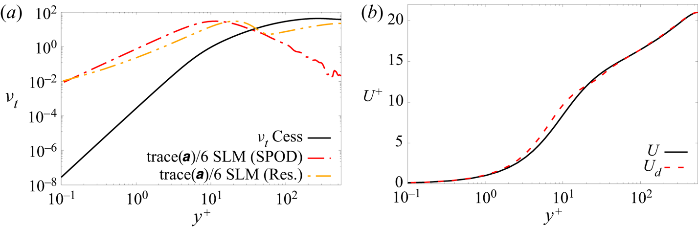
The constant $K=100$ allows us to obtain an order of magnitude of ${\boldsymbol{\mathsf{a}}}$ consistent with Cess's eddy viscosity. This value, selected by inspection of figure 1(a), has been determined in terms of order of magnitude and not based on a fine iterative tuning. A very low order of magnitude for $K$ leads to disappearance of the effects of stochastic diffusion and drift velocity, and a very large order of magnitude leads to unphysical results dominated by the noise.

Figure 1.

Effect on the stochastic diffusion and the drift velocity at $Re=550$: (a) diffusion and (b) drift velocity.

The fact that SPOD modes are purely coherent modes decorrelated from each other justifies the expansion (4.22) by randomising the expansion coefficients.

It should be remarked that this definition of the operator $\sigma$ requires a complete time-resolved dataset in order to be able to compute the SPOD, which is per se an intensive post-processing procedure.

4.3.2. Based on resolvent analysis

As a second approach, we use $\nu$-resolvent analysis to build the background turbulence statistics $\sigma$ at the considered frequency-wavenumber combination. This amounts to considering an imperfect prediction based on the resolvent, with the simplifying assumption of nonlinear terms as spatial white noise, to build a first estimate of the turbulence statistics, which are subsequently taken to define the coloured Brownian motion statistics $\sigma$ in our model. In that perspective, a distinction is made between the linear response to generalized Reynolds stresses modelling the background turbulence $\boldsymbol {\sigma } \,\mathrm {d}\boldsymbol {B}_t$ and the linear wave sustained by this background turbulence $\hat {\boldsymbol {q}}_{\alpha ,\beta ,\omega }$.

With this underlying idea, we define, similarly as for the SPOD noise,

(4.24)\begin{equation} {\boldsymbol{\mathsf{a}}}^{\textit{resolvent}}(y)= \left(A_{r}\sum_{j=1}^{N_{\textit{resolvent}}}\boldsymbol{\varPhi}_{j,\alpha\beta\omega}^{\textit{resolvent}}(y) (s_{j,\alpha\beta\omega}^{\textit{resolvent}})^2 (\boldsymbol{\varPhi}_{j,\alpha\beta\omega}^{\textit{resolvent}}(y))^*+A_b\mathbb{I}\right)\tau, \end{equation}

and

(4.25)\begin{equation} (\dot{\boldsymbol{\xi}}_{\alpha,\beta,\omega})^{\textit{resolvent}}= A_r^{1/2}\sum_{j=1}^{N_{\textit{resolvent}}}\boldsymbol{\varPhi}_{j,\alpha \beta\omega}^{\textit{resolvent}}(y){s_{j,\alpha\beta\omega}^{\textit{resolvent}}} \dot{\eta}_j+A_b^{1/2}\dot{\boldsymbol{\eta}}^{ \textit{background}}.\end{equation}

The constant $A_r$ is a global amplitude that is a free parameter. For reasons of consistency with the data-driven noise defined from SPOD, we choose $A_r^{1/2}=\sqrt {\lambda _{1,\alpha \beta \omega }^{\textit{SPOD}}}/s_{1,\alpha \beta \omega }^{\textit{resolvent}}$. This sets the noise amplitude from data, but it could be considered as well as a single free parameter in a fully model-based perspective. The resolvent predictions were obtained without inclusion of an eddy viscosity to avoid a circular nature of the model; the resolvent only provides an estimate of the stochastic field, which will subsequently be used to force the waves and modify the linearised operator via the drift velocity and the stochastic diffusion.

Moreover, it has been observed that an additional constant background noise is necessary to represent fluctuations in the middle of the channel (structures exemplified by wave 2 as defined in § 5), present with SPOD noise, but missing with resolvent noise. The constant $A_b=1/\tau$ is chosen in order to obtain comparable levels to Cess's model in the middle of the channel. The noise term $\dot {\boldsymbol {\eta }}^{\textit{background}}$ denotes here a centred standard white noise field. The modelling is designed to mimic the behaviour of SPOD noise, and refinement of the definition of $\sigma$ is an open research direction.

5.1. Effect of the variance tensor

As a first analysis, we show here the effect of the tensor ${\boldsymbol{\mathsf{a}}}$, through the stochastic diffusion and the drift velocity. In figure 1(a) we compare 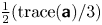$\frac {1}{2}({\text {trace}({\boldsymbol{\mathsf{a}}})}/{3})$ of wave 1 at $Re_\tau =550$ with Cess’ eddy viscosity $\nu _t$. Compared with Cess’ model that leads to an eddy viscosity that increases monotonically with wall distance, so as to lead to the mean velocity profile of the channel, SPOD and resolvent noise lead to large diffusion in the buffer layer around $y^+\approx 10$, where the SPOD modes peak. It was observed that the eddy viscosity/stochastic diffusion in the channel centre plays a significant role in the stochastic linearised mode's shape. Indeed, SPOD noise leads to good results, but resolvent noise without adding the background homogeneous noise showed a faster decay in the channel centre, which we believe to be the reason of failure. This is the reason why we have added an additional homogeneous noise in the resolvent noise (4.24) and (4.25), such that the level of induced stochastic diffusion is comparable to $\nu _t$. The effect of this noise can be shown for $y^+>100$ in the resolvent noise, and that constitutes the main difference between both noises. Let us note however that the stochastic model should not be interpreted as more diffusive than Cess’ model. As a matter of fact, the noise which acts globally as a backscatering term is counterbalanced by the (negative) stochastic diffusion energy.

In figure 1(b) we compare the mean flow profile $U(y)$ with the mean drift velocity profile $U_d(y)$ at $Re_\tau =550$ with the SPOD noise of wave 1. The main effect of the corrective drift is around $y^+=10$, which is consistent with the study of Pinier et al. (Reference Pinier, Mémin, Laizet and Lewandowski2019) showing that the stochastic transport formalism has a large influence in the buffer layer.

5.2. Comparison with SPOD modes from the DNS databases

The linear stochastic modes are compared with results of resolvent analysis, described in § 3.2. These models are discretised with 128 (respectively 256) Chebyshev polynomials at $Re_{\tau }=180$ (respectively $Re_{\tau }=550$), the same number of polynomials used in the DNS. The accuracy of SLMs in modelling coherent structures in turbulent channel flows is evaluated by comparing results to SPOD modes from the two channels. The two choices of noise presented in § 4.3 are tested. For all the results, the two leading modes from SPOD, resolvent analysis and the linearised stochastic model are considered. They are referred to respectively as mode 1 and mode 2. Higher-order modes are not shown in order to avoid any misinterpretation due to numerical convergence of the SPOD, which requires very long time series for higher-order modes (Lesshafft et al. Reference Lesshafft, Semeraro, Jaunet, Cavalieri and Jordan2019). Stochastic linearised modes are obtained using an ensemble of $N_{{ens}}=10\ 000$ members. In practice, $1000$ members are enough to obtain robust results, and we have increased this value to eliminate any doubt of convergence.

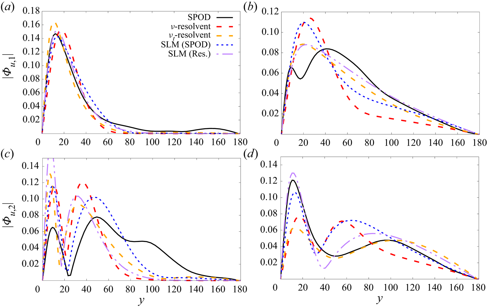
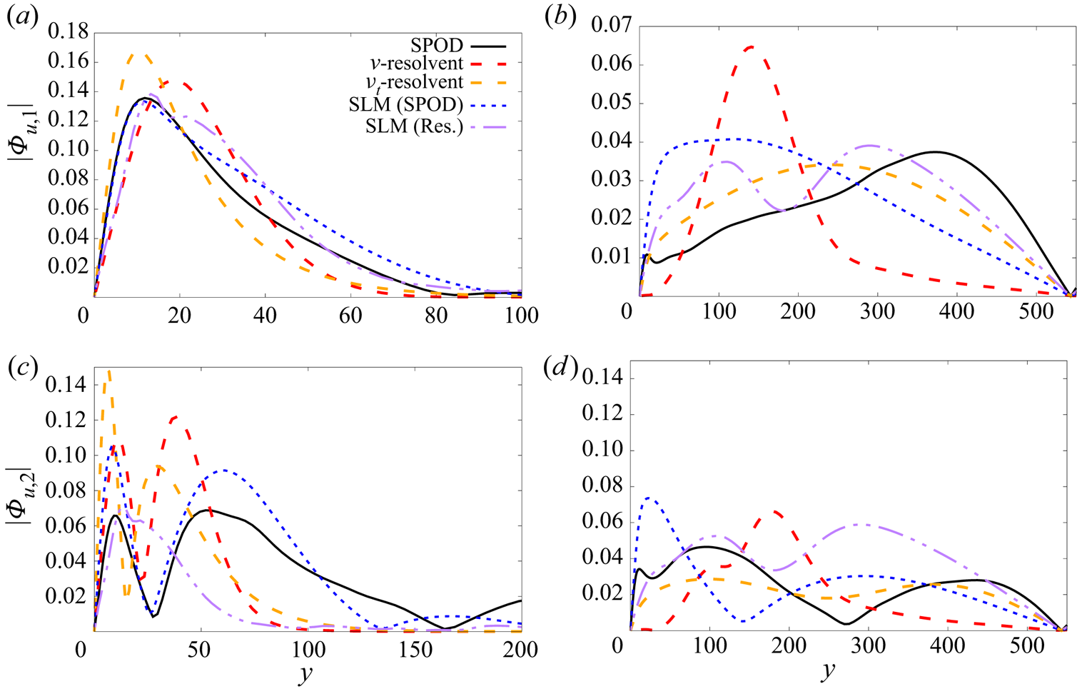
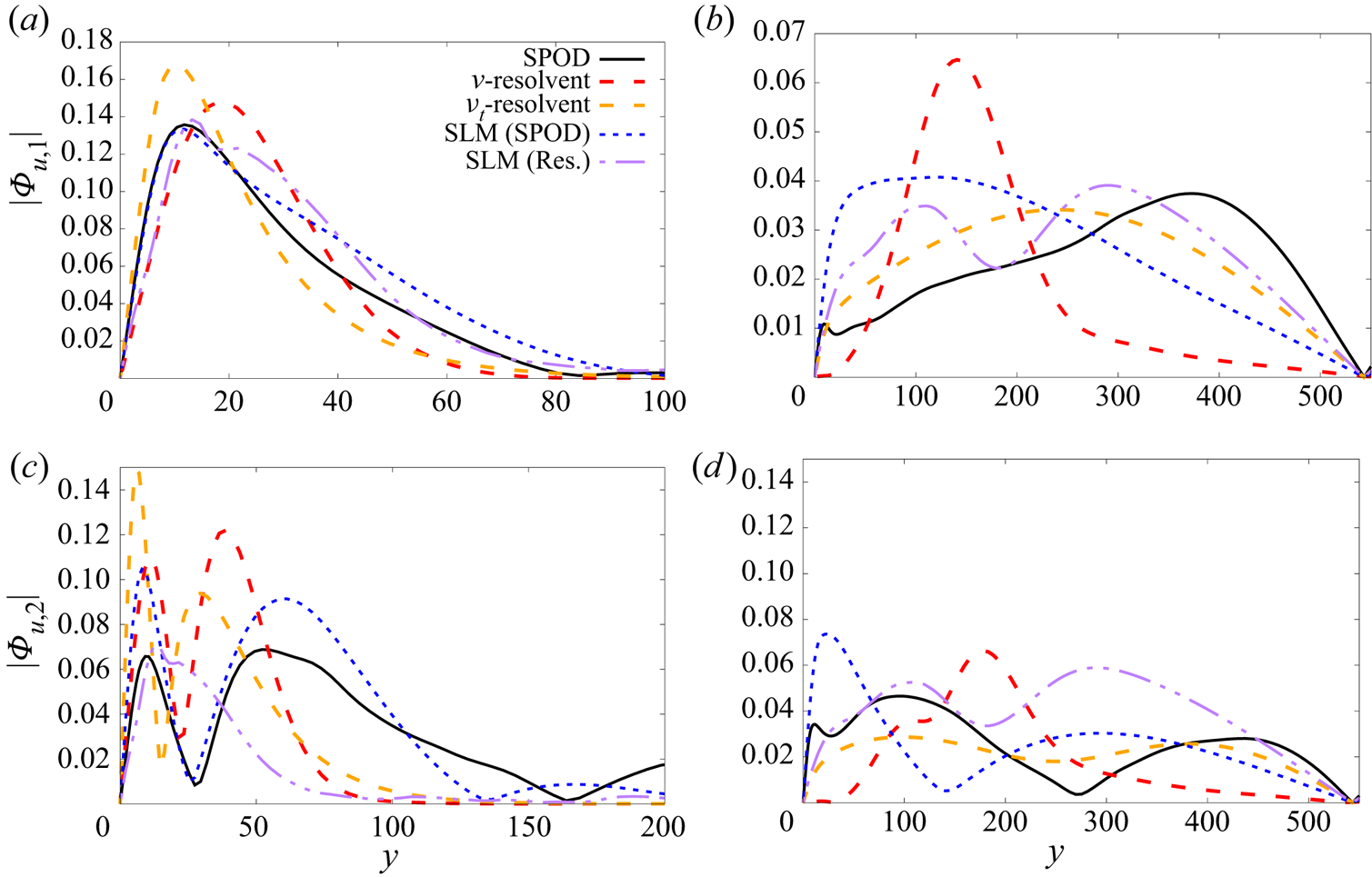
Figures 2 and 3 show mode amplitudes for $Re_{\tau }=180$ and $Re_{\tau }=550$, respectively. Recall that the wall-normal coordinate $y$ is expressed in inner units. Two typical waves are presented. The first one, denoted ‘wave 1’, is typical of a streaky structure ($\lambda _x^+\approx 10 \lambda _z^+$) representative of the near-wall cycle (Jiménez Reference Jiménez2013), for which the resolvent analysis is predictive (Abreu et al. Reference Abreu, Cavalieri, Schlatter, Vinuesa and Henningson2020a,b). The second one, denoted ‘wave 2’, has a similar phase speed, but is of larger size with a lower aspect ratio $\lambda _x^+\approx 2 \lambda _z^+$. In the latter case, the turbulent structures are larger and extend further from the wall. For this type of wave, resolvent analysis shows significant discrepancies compared with the reference SPOD modes. Exact values of wavelengths are given in the figure captions. We have $\alpha ={2{\rm \pi} }/{\lambda _x^+}$, $\beta ={2{\rm \pi} }/{\lambda _z^+}$ and $\omega ={2{\rm \pi} }/{\lambda _t^+}$, where $\lambda _x^+$ and $\lambda _z^+$ denote wavelengths in the $x$ and $z$ directions, respectively, and $\lambda _t^+$ is the time period, with all results expressed in inner units. Only antisymmetric waves (in $u$) with respect to the channel centreline are displayed. Such antisymmetric modes can be obtained by restricting the forcing in resolvent and stochastic models to be antisymmetric, and by taking the antisymmetric part of disturbances prior to computing SPOD. Similar analysis for symmetric waves shows similar results and will not be shown here for conciseness. Results are shown here for the $u$ component, and corresponding results for $v$ and $w$ can be found in appendix B.

Figure 2.

Profiles of the power spectral density of $|\hat {u}|$ at $Re_{\tau }=180$ for two waves: (a) wave 1, mode 1, $u$; (b) wave 2, mode 1, $u$; (c) wave 1, mode 2, $u$; (d) wave 2, mode 2, $u$. Wave 1: $\lambda _x^+=1124$, $\lambda _z^+=102$, $\lambda _t^+=100$; wave 2: $\lambda _x^+=2249$, $\lambda _z^+=1124$, $\lambda _t^+=200$. Spectral POD (black), $\nu$-resolvent modes (red), $\nu _t$-resolvent (orange), SLM with a noise defined by SPOD (blue) and resolvent (purple).

Figure 3.

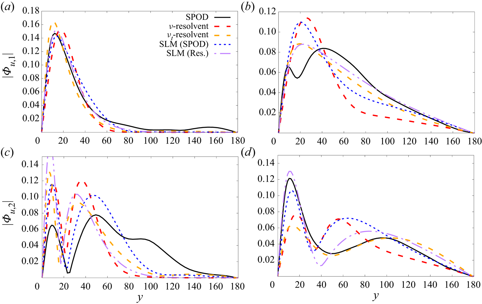
Profiles of the power spectral density of $|\hat {u}|$ at $Re_{\tau }=550$ for three waves: (a) wave 1, mode 1, $u$; (b) wave 2, mode 1, $u$; (c) wave 1, mode 2, $u$; (d) wave 2, mode 2, $u$. Wave 1: $\lambda _x^+=1137$, $\lambda _z^+=100$, $\lambda _t^+=100$; wave 2: $\lambda _x^+=3412$, $\lambda _z^+=1706$, $\lambda _t^+=200$. Spectral POD (black), $\nu$-resolvent modes (red), $\nu _t$-resolvent (orange), SLM with a noise defined by SPOD (blue) and resolvent (purple).

Considering wave $1$ at $Re_\tau =180$ in figures 2(a) and 2(c), $\nu$-resolvent analysis is able to reproduce SPOD with a good accuracy. For this kind of wave, the improvement margin is quite low. In accordance with previous results in the literature, such as Morra et al. (Reference Morra, Semeraro, Henningson and Cossu2019), incorporating the eddy viscosity in the resolvent analysis slightly improves further the agreement with SPOD. 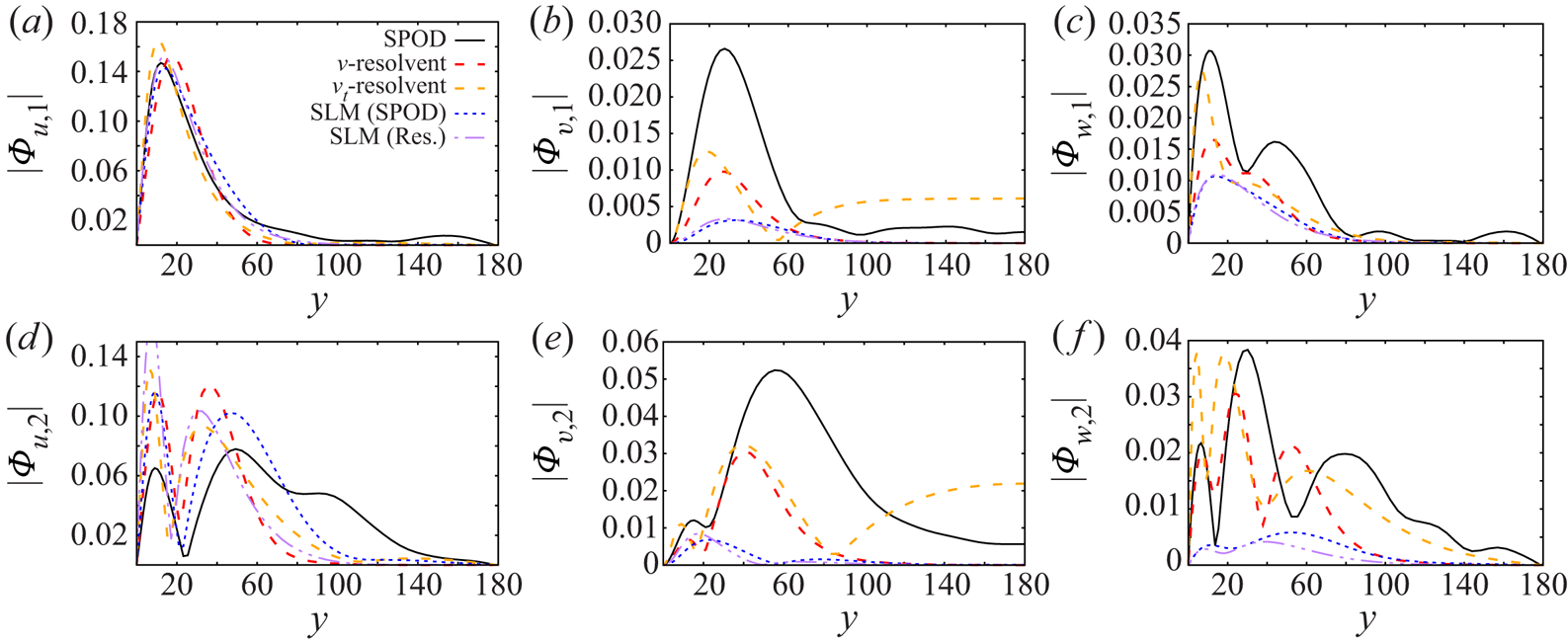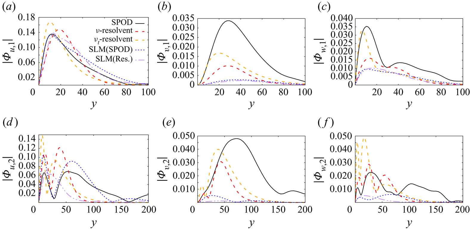Stochastic linearised models with a noise based either on SPOD or resolvent modes have similar performances than $\nu _t$-resolvent to recover the first SPOD mode. In the appendix it is shown in figure 9 that for wave $1$, the SLM is slightly better to predict $u$ than $\nu _t$-resolvent, and leads to a slight worsening for $v$ and $w$. We can note a very good agreement of SLM with resolvent noise to predict $u$. The hierarchy of performances is less clear for mode $2$, except that SLM with a SPOD noise improves significantly the prediction of $u$.

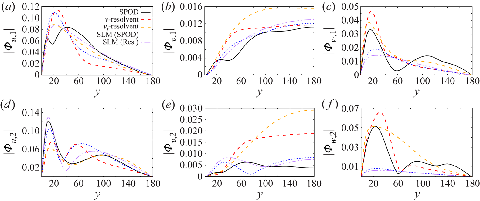
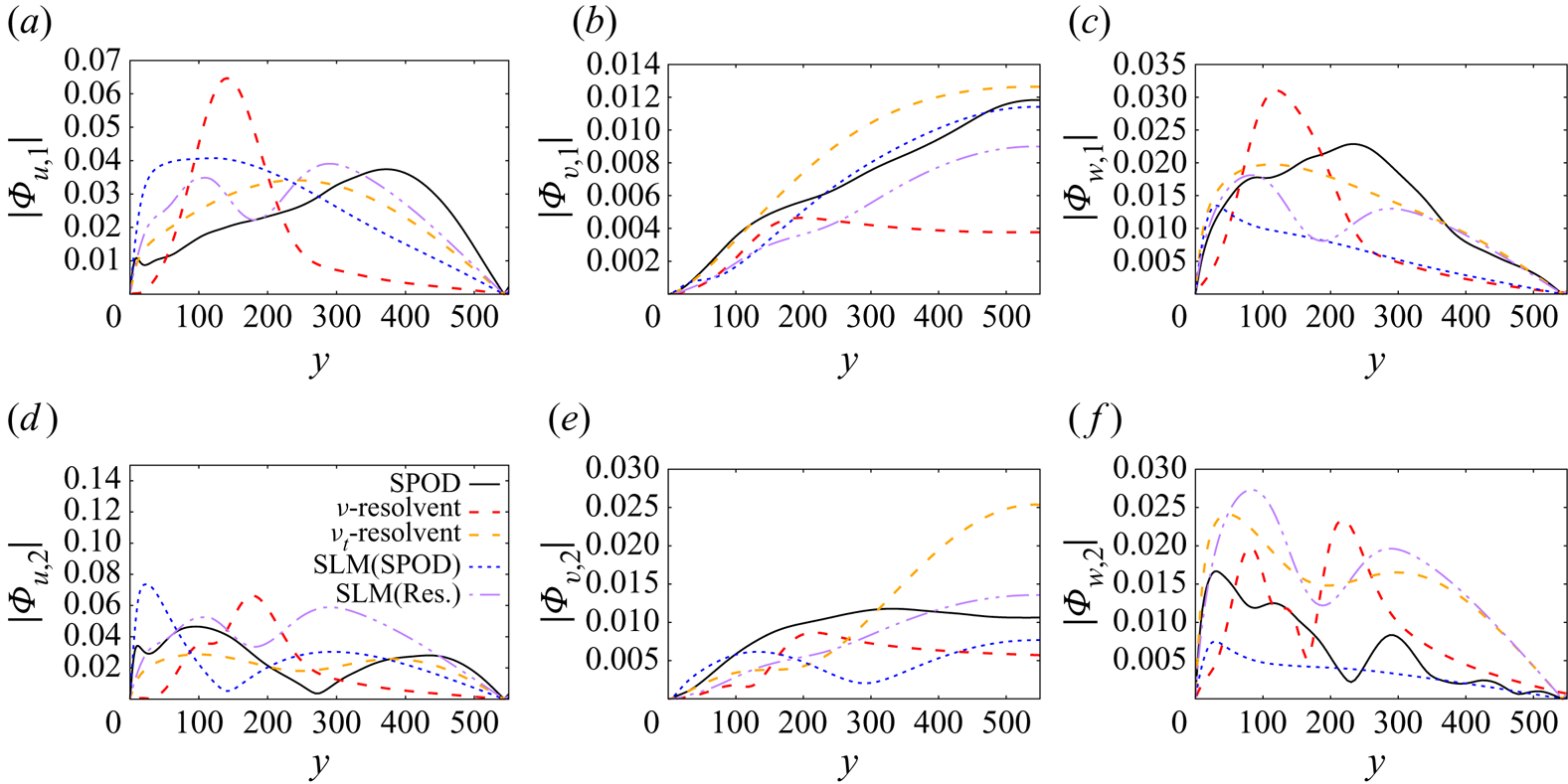
For wave $2$ in figures 2(b) and 2(d), where $\nu$-resolvent shows large discrepancies, the eddy viscosity improves well the behaviour. In that situation, SLM improves the agreement, especially for the noise based on resolvent analysis. In figure 10 in the appendix, it can be shown that the improvement of $v$ predictions is strong. This can be explained by the fact that the forcing shape (4.20) comes for the term coupling velocity components $\tilde {f}_x=-(\hat {\boldsymbol {\sigma }}\dot {\boldsymbol {\eta }}_{\alpha ,\beta ,\omega })_y (\partial U / \partial y)$. The improvement is more pronounced for mode $2$.

Comparison of the results in figures 2 and 3 shows that the performance of SLM at $Re_{\tau }=550$ is quite similar to what is obtained for $Re_{\tau }=180$. Exactly the same analysis can be done on wave $1$. This gives us some confidence on the robustness of the modelling procedure. Wave $2$, figure 3(b), is slightly different since it extends more in the centre of the channel, from the lower $Re_\tau$ results, as it represents larger structures extending to higher wall-normal locations, more relevant for larger Reynolds numbers. In this case, the disagreement between $\nu$-resolvent analysis and SPOD is amplified. The $\nu _t$-resolvent finds a solution with a wider extend but located too close to the wall. A SLM with SPOD seems to find a solution of the same nature than $\nu _t$-resolvent, but SLM with resolvent noise begins to have large values near the centre of the channel. This supports the importance of modelling properly the noise statistics in the centre of the channel.

5.3. Comparison of cross-spectral densities

For a more complete view, the CSD ${\boldsymbol{\mathsf{S}}}_{\alpha ,\beta ,\omega }(y,y')= \mathbb {E}(\hat {\boldsymbol {u}}_{\alpha ,\beta ,\omega }(y)\hat {\boldsymbol {u}}_{\alpha ,\beta ,\omega }(y'))$ can be compared. This matrix is already computed to obtain SPOD (from the DNS data) and stochastic model (by the construction of an ensemble of realisations). As for the resolvent operator, assuming the system is excited by a Gaussian white noise, the CSD can be predicted (Cavalieri et al. Reference Cavalieri, Jordan and Lesshafft2019) by

(5.1)\begin{equation} {\boldsymbol{\mathsf{S}}}^{{\textit{resolvent}}}_{\alpha,\beta,\omega}={\boldsymbol{\mathsf{R}}}_{\alpha,\beta,\omega} \mathbb{E}(\,\hat{\boldsymbol{f}}_{\alpha,\beta,\omega}\,\hat{\boldsymbol{f}}_{\alpha,\beta,\omega}^*) {\boldsymbol{\mathsf{R}}}_{\alpha,\beta,\omega}^*={\boldsymbol{\mathsf{R}}}_{\alpha,\beta, \omega}{\boldsymbol{\mathsf{R}}}_{\alpha,\beta,\omega}^*. \end{equation}

Focusing on wave $1$ at $Re_\tau =180$, the CSD matrix is compared in figure 4. Only the streamwise component $S^{uu}_{\alpha ,\beta ,\omega }(y,y')=\mathbb {E}(\hat {u}_{\alpha , \beta ,\omega }(y)\hat {u}_{\alpha ,\beta ,\omega }(y'))$ is shown for the sake of conciseness. It can be shown that $\nu$-resolvent analysis predicts a too short coherence decay (seen by small values at off-diagonal terms in the CSD), with an elliptic pattern in the CSD, while the SPOD have rather a guitar plectrum shape. The prediction with $\nu _t$-resolvent is more accurate, but the non-ellipticity is too pronounced. Both SLMs improve significantly the prediction.

Figure 4.

Real part of $S^{uu}_{\alpha ,\beta ,\omega }(y,y')$ for wave 1 $\lambda _x^+=1137$, $\lambda _z^+=100$, $\lambda _t^+=100$ at $Re_{\tau }=180$: (a) spectral POD, (b) $\nu$-resolvent, (c) $\nu _t$-resolvent, (d) SLM (SPOD) and (e) SLM (Res.).

5.4. Collinearity metric

A comprehensive view of the modelling performances over all scales can be given by a collinearity criteria

(5.2)\begin{equation} \beta^{{model}}_{j,\alpha,\beta,\omega}=\frac{|(\boldsymbol{\varPhi}^{{model}}_{j, \alpha,\beta,\omega},\boldsymbol{\varPhi}_{j,\alpha,\beta, \omega}^{\textit{SPOD}})|}{\|\boldsymbol{\varPhi}^{{model}}_{j,\alpha,\beta,\omega} \|\|\boldsymbol{\varPhi}_{j,\alpha,\beta,\omega}^{\textit{SPOD}}\|}, \end{equation}

defined similarly as in Cavalieri et al. (Reference Cavalieri, Rodriguez, Jordan, Colonius and Gervais2013), Lesshafft et al. (Reference Lesshafft, Semeraro, Jaunet, Cavalieri and Jordan2019) and Abreu et al. (Reference Abreu, Cavalieri, Schlatter, Vinuesa and Henningson2020b). As a reference, figure 5 represents the collinearity between SPOD and eddy resolvent analysis for all wavelengths at $\lambda _t^+=200$ and $\lambda _t^+=1000$ for $Re_\tau =180$. It shows that, in agreement with the analysis of turbulent pipe flow by Abreu et al. (Reference Abreu, Cavalieri, Schlatter, Vinuesa and Henningson2020b) (performed for $\nu$-resolvent), the first $\nu _t$-resolvent mode predicts well the first SPOD modes for a wide range of wavelengths, especially for elongated modes ($\lambda _x^+>\lambda _z^+$), exemplified previously by wave 1. There is very little room for improvement in those regimes. The accuracy decreases for less elongated modes, of larger size and with a lower frequency (large $\lambda _z^+$ and $\lambda _t^+$, low $\lambda _x^+$), exemplified by wave $2$. In all cases, the second $\nu _t$-resolvent mode leads to poor predictions of the second SPOD mode. First SPOD eigenvalues in figures 5(c) and 5(g) are shown to evaluate the presence of these structures in the flow in terms of kinetic energy. A similar behaviour is shown in appendix C for $Re_\tau =550$ (figure 13). The worse agreement between SPOD and $\nu _t$-resolvent is directly associated with the decay of the ratio of the two first $\nu _t$-resolvent singular values (see figures 5d and 5h). Such cases require a finer description of the noise for accurate modelling.

Figure 5.

Value of $\beta ^{{{\nu _t\textit{-resolvent}}}}_{j,\alpha ,\beta ,\omega }$ at $Re_{\tau }=180$ measuring the accordance between $\nu _t$-resolvent analysis and SPOD. (a) Value of $\beta ^{{{\nu _t\textit{-resolvent}}}}_{j,\alpha ,\beta ,\omega }$, mode 1, $\lambda _t^+=200$. (b) Value of $\beta ^{{{\nu _t\textit{-resolvent}}}}_{j,\alpha ,\beta ,\omega }$, mode 2, $\lambda _t^+=200$. (c) First SPOD eigenvalue $\log _{10}(\lambda _1)$ for $\lambda _t^+=200$. (d) Ratio $s_1^2/s_2^2$ of the $\nu _t$-resolvent singular values for $\lambda _t^+=200$. (e) Value of $\beta ^{{{\nu _t\textit{-resolvent}}}}_{j,\alpha ,\beta ,\omega }$, mode 1, $\lambda _t^+=1000$. (f) Value of $\beta ^{{{\nu _t\textit{-resolvent}}}}_{j,\alpha ,\beta ,\omega }$, mode 2, $\lambda _t^+=1000$. (g) First SPOD eigenvalue $\log _{10}(\lambda _1)$ for $\lambda _t^+=1000$. (h) Ratio $s_1^2/s_2^2$ of the $\nu _t$-resolvent singular values for $\lambda _t^+=1000$.

Figure 6 compares $\beta ^{{\nu _t\textit{-resolvent}}}_{j,\alpha ,\beta ,\omega }$, $\beta ^{\textit{SLM (SPOD)}}_{j,\alpha ,\beta ,\omega }$ and $\beta ^{\textit{SLM (Res.)}}_{j,\alpha ,\beta ,\omega }$ at $Re_{\tau }=180$ and $\lambda _t^+=200$. We can see that for elongated waves, where $\nu _t$-resolvent is highly performant, SLM has slightly lower agreement metrics, but there is a clear improvement to match SPOD at wavenumbers for which $\nu _t$-resolvent is less efficient.

Figure 6.

Value of $\beta ^{{\nu _t\textit{-resolvent}}}_{j,\alpha ,\beta ,\omega }$, $\beta ^{\textit{SLM (SPOD)}}_{j,\alpha ,\beta ,\omega }$ and $\beta ^{\textit{SLM (Res.)}}_{j,\alpha ,\beta ,\omega }$ at $Re_{\tau }=180$ and $\lambda _t^+=200$ measuring the accordance between the respective models and SPOD. (a) Mode 1, $\nu _t$-resolvent. (b) Mode 1, SLM (SPOD). (c) Mode 1, SLM (Res.). (d) Mode 2, $\nu _t$-resolvent. (e) Mode 2, SLM (SPOD). (f) Mode 2, SLM (Res.).

In order to quantify the improvement (in terms of SPOD predictability) brought by the stochastic model compared with $\nu _t$-resolvent, we define the log-ratio of collinearity criteria

(5.3)\begin{equation} \gamma_{j,\alpha,\beta,\omega}^{\textit{SLM noise}}=\log \left(\frac{\beta^{\textit{SLM noise}}_{j,\alpha,\beta, \omega}}{\beta^{{{\nu_t\textit{-resolvent}}}}_{j,\alpha,\beta,\omega}}\right). \end{equation}

The label ‘SLM noise’ refers to the noise definition of the stochastic linearised model. It can be defined by SPOD (SLM SPOD) or resolvent (SLM Res.). Figures 7 and 8 show $\gamma _{j,\alpha ,\beta ,\omega }^{\textit{SLM noise}}$ respectively at $Re_\tau =180$ and $Re_\tau =550$, for $\lambda _t^+=200$. Other frequencies are displayed in appendix C (figures 14–17). In all these figures, red (blue) regions show parameters where SLM leads to better (worse) predictions compared with $\nu _t$-resolvent predictions.

Figure 7.

Value of $\gamma _{j,\alpha ,\beta ,\omega }^{\textit{SLM noise}}$, $Re_{\tau }=180$, $\lambda _t^+=200$. (a) Mode 1, SLM (SPOD). (b) Mode 1, SLM (Res.). (c) Mode 2, SLM (SPOD). (d) Mode 2, SLM (Res.).

Figure 8.

Value of $\gamma _{j,\alpha ,\beta ,\omega }^{\textit{SLM noise}}$, $Re_{\tau }=550$, $\lambda _t^+=200$. (a) Mode 1, SLM (SPOD). (b) Mode 1, SLM (Res.). (c) Mode 2, SLM (SPOD). (d) Mode 2, SLM (Res.).

Figure 9.

Profiles of the power spectral density at $Re_{\tau }=180$ for wave 1: $\lambda _x^+=1124$, $\lambda _z^+=102$, $\lambda _t^+=100$. Spectral POD (black), $\nu$-resolvent modes (red), $\nu _t$-resolvent (orange), SLM with a noise defined by SPOD (blue) and resolvent (purple). (a) Mode 1, $|\hat {u}|$. (b) Mode 1, $|\hat {v}|$. (c) Mode 1, $|\hat {w}|$. (d) Mode 2, $|\hat {u}|$. (e) Mode 2, $|\hat {v}|$. (f) Mode 2, $|\hat {w}|$.

Figure 10.

Profiles of the power spectral density at $Re_{\tau }=180$ for wave 2: $\lambda _x^+=3412$, $\lambda _z^+=1706$, $\lambda _t^+=200$. Spectral POD (black), $\nu$-resolvent modes (red), $\nu _t$-resolvent (orange), SLM with a noise defined by SPOD (blue) and resolvent (purple). (a) Mode 1, $|\hat {u}|$. (b) Mode 1, $|\hat {v}|$. (c) Mode 1, $|\hat {w}|$. (d) Mode 2, $|\hat {u}|$. (e) Mode 2, $|\hat {v}|$. (f) Mode 2, $|\hat {w}|$.

As a first remark, for all Reynolds numbers and frequencies and for both noise definitions, the trend described previously is confirmed, i.e. an improvement (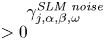$\gamma _{j,\alpha ,\beta ,\omega }^{\textit{SLM noise}} >0$) at wavenumbers for which $\nu _t$-resolvent has moderate performances, and a slight performance loss for elongated waves. Moreover, the improvement is generally better for mode 2. Let us remark that for these elongated waves, the agreement is still good, and better than $\nu$-resolvent analysis, as it has been shown by the profiles of wave 1. Considering the choice of the noise, SLM (SPOD) is a reference case, where the noise is defined from DNS data. Resolvent noise SLM (Res.) is a model-based technique whose goal is to approach the SPOD noise performance. In the latter case, the improvement follows the same trend than the one with SPOD noise, with a slightly lower performance (especially at $Re_\tau =550$) than the one that can be expected since the modelling is now purely model based. Resolvent modelling thus constitutes a robust and efficient way to define the noise. It clearly improves the performances of the resolvent analysis while remaining purely based on the model. Obviously, if SPOD modes are available, it is preferable to use them.