1. Introduction
In recent years, annually resolved radiocarbon measurements from tree rings have opened new avenues for exploring short-timescale fluctuations and, by extension, past solar activity and cosmic-ray events. Extreme anomalies such as those dated to AD 774–775 and AD 993–994 are now widely recognized as signatures of solar nuclei, expelled during exceptionaly intense solar flares (e.g., Jull et al. Reference Jull, Panyushkina, Lange, Kukarskih, Myglan, Clark, Salzer, Burr and Leavitt2014; Miyake et al. Reference Miyake, Masuda and Nakamura2013; Miyake et al. Reference Miyake, Nagaya, Masuda and Nakamura2012; Usoskin et al. Reference Usoskin, Kromer, Ludlow, Beer, Friedrich, Kovaltsov, Solanki and Wacker2013). They have proven extremely valuable for anchoring historical and archaeological chronologies with annual precision (Kuitems et al. Reference Kuitems, Wallace, Lindsay, Scifo, Doeve, Jenkins, Lindauer, Erdil, Ledger, Forbes, Vermeeren, Friedrich and Dee2022). Such events appear as sharp “spikes” by which to align independent archives, the causal mechanisms and recording pathways involved remaining the subject of debate.
The reproducibility and synchronicity of these signals across geographically distant records have raised broader questions regarding the spatial distribution of 14C production and its atmospheric propagation. A growing number of annually-resolved datasets have been developed from the Northern Hemisphere, primarily from mid to high-latitude tree-ring archives in Japan, North America, and western Europe (e.g., Büntgen et al. Reference Büntgen, Wacker, Galván, Arnold, Arseneault, Baillie, Beer, Bernabei, Bleicher, Boswijk, Bräuning, Carrer, Ljungqvist, Cherubini, Christl, Christie, Clark, Cook, D’Arrigo, Davi, Eggertsson, Esper, Fowler, Gedalof, Gennaretti, Grießinger, Grissino-Mayer, Grudd, Gunnarson, Hantemirov, Herzig, Hessl, Heussner, Jull, Kukarskih, Kirdyanov, Kolář, Krusic, Kyncl, Lara, LeQuesne, Linderholm, Loader, Luckman, Miyake, Myglan, Nicolussi, Oppenheimer, Palmer, Panyushkina, Pederson, Rybníček, Schweingruber, Seim, Sigl, Churakova (Sidorova), Speer, Synal, Tegel, Treydte, Villalba, Wiles, Wilson, Winship, Wunder, Yang and Young2018; Pearson et al. Reference Pearson, Brewer, Brown, Heaton, Hodgins, Jull, Lange and Salzer2018; Uusitalo et al. Reference Uusitalo, Arppe, Hackman, Helama, Kovaltsov, Mielikainen, Makinen, Nojd, Palonen, Usoskin and Oinonen2018). In contrast, similar data from low-latitude and Southern Hemisphere regions remain rare. This geographic imbalance limits both our ability to test models of cosmogenic isotope distribution and to refine the southern calibration curve (SHCal; Hogg et al. Reference Hogg, Heaton, Hua, Palmer, Turney, Southon, Bayliss, Blackwell, Boswijk, Bronk Ramsey, Pearson, Petchey, Reimer, Reimer and Wacker2020), which is currently based on very little of its data from SH tree-ring data, with the remainder inferred from IntCal after applying a 36 + 27 14C year offset. Several studies have suggested that the amplitude of 14C events recorded in tree rings may vary with latitude, as a response to the modulating effect of the Earth’s magnetic field on incoming high-energy particles (e.g., Büntgen et al. Reference Büntgen, Wacker, Galván, Arnold, Arseneault, Baillie, Beer, Bernabei, Bleicher, Boswijk, Bräuning, Carrer, Ljungqvist, Cherubini, Christl, Christie, Clark, Cook, D’Arrigo, Davi, Eggertsson, Esper, Fowler, Gedalof, Gennaretti, Grießinger, Grissino-Mayer, Grudd, Gunnarson, Hantemirov, Herzig, Hessl, Heussner, Jull, Kukarskih, Kirdyanov, Kolář, Krusic, Kyncl, Lara, LeQuesne, Linderholm, Loader, Luckman, Miyake, Myglan, Nicolussi, Oppenheimer, Palmer, Panyushkina, Pederson, Rybníček, Schweingruber, Seim, Sigl, Churakova (Sidorova), Speer, Synal, Tegel, Treydte, Villalba, Wiles, Wilson, Winship, Wunder, Yang and Young2018). Trees growing at higher geomagnetic latitudes may receive a larger flux of cosmic rays, leading to a stronger local 14C signal. However, this interpretation remains debated. For instance, modeling studies (Zhang et al. Reference Zhang, Sharma, Dennis, Scifo, Kuitems, Büntgen, Owens, Dee and Pope2022) have challenged the assumption that production rates differ significantly by latitude, pointing instead to post-production processes such as atmospheric mixing or archive-specific responses as possible sources of signal modulation. So far, Northern Hemisphere 14C raw datasets have not shown a clear correlation with latitude.
In addition to potential spatial differences in production, regional variations in atmospheric 14C are primarily governed by post-production processes. Following their production in the stratosphere, cosmogenic 14C atoms remains there for roughly 0.5–1 year before being transferred into the troposphere (Bard et al. Reference Bard, Raisbeck, Yiou and Jouzel1997; Levin and Hesshaimer, Reference Levin and Hesshaimer2000). Once in the troposphere, the signal is further damped and delayed by interhemispheric atmospheric exchange, which typically requires 1–2 years (Braziunas et al. Reference Braziunas, Fung and Stuiver1995; Tans et al. Reference Tans, De Jong and Mook1979), explaining regional offsets between records. Superimposed upon these transport effects, air–sea CO2 exchanges modulate atmospheric 14C both hemispherically and locally, especially in regions of intense upwelling, which release 14C-depleted CO2 (Naegler et al. Reference Naegler, Ciais, Rodgers and Levin2006). At finer spatial scales, variations in canopy structure, soil respiration, and local CO2 turnover can perturb atmospheric 14C (Levin and Hesshaimer Reference Levin and Hesshaimer2000). Such effects are even more pronounced since historical times due to land-use changes, including deforestation and agriculture. Additionally, since the onset of the industrial era, the progressive combustion of 14C-free fossil fuels has globally decreased atmospheric 14C/C ratio (Suess effect) which also exhibits spatial gradients depending on proximity to industrial sources (Graven et al. Reference Graven, Guilderson and Keeling2012; Suess Reference Suess1955). Finally, biophysiological processes in trees can also alter the amplitude and timing of the recorded signal; the timing of the occurrence of the event relative to the growing season, and the phenology and carbon allocation strategies characteristic of each species further modulate the imprint of atmospheric excursons (Kagawa et al. Reference Kagawa, Sugimoto and Maximov2006; Svarva et al. Reference Svarva, Grootes, Seiler and Nadeau2025; Uusitalo et al. Reference Uusitalo, Arppe, Hackman, Helama, Kovaltsov, Mielikainen, Makinen, Nojd, Palonen, Usoskin and Oinonen2018).
Given this context, high-quality 14C data from the SH are crucial to resolve current uncertainties. To help fill this gap, we launched the MITI-CHASCA project, designed to develop an annually resolved radiocarbon record from Fitzroya cupressoides (RAL060 dendro series), a long-lived conifer endemic to southern South America. The resulting CHASCA dataset spans AD 970–1084 and represents the first annual 14C data from South America and one of the longest records available for the Southern Hemisphere.
2. Material and methods
2.1 Material
Fitzroya cupressoides is an emblematic, endemic species of the temperate Andean-Patagonian forests, notable for its large size and exceptional longevity. Under optimal conditions, it can exceed 50 m in height and 4 m in diameter, with some individuals reaching ages of over 3600 years, making it the longest-lived tree species in the Southern Hemisphere, surpassed globally only by Pinus longaeva (Lara and Villalba Reference Lara and Villalba1993). Its current distribution is discontinuous, extending between 39.80 ºS and 43.50 ºS, primarily concentrated in Chile and, to a lesser extent, in Argentina (Donoso Zegers Reference Donoso Zegers1993). Transverse wedges from F. cupressoides stumps remaining from historical logging (prior to 1935) were collected between 2015 and 2019 in the Los Alerces River Valley, Los Alerces National Park, Argentina (42.74 ºS, 72.01 ºW; Figure 1).
Location of the CHASCA series (red star). Two additional series available in the literature are shown for comparison: Dargaville, New Zealand (blue star) and El Siento, Chile (orange star) (Büntgen et al. Reference Büntgen, Wacker, Galván, Arnold, Arseneault, Baillie, Beer, Bernabei, Bleicher, Boswijk, Bräuning, Carrer, Ljungqvist, Cherubini, Christl, Christie, Clark, Cook, D’Arrigo, Davi, Eggertsson, Esper, Fowler, Gedalof, Gennaretti, Grießinger, Grissino-Mayer, Grudd, Gunnarson, Hantemirov, Herzig, Hessl, Heussner, Jull, Kukarskih, Kirdyanov, Kolář, Krusic, Kyncl, Lara, LeQuesne, Linderholm, Loader, Luckman, Miyake, Myglan, Nicolussi, Oppenheimer, Palmer, Panyushkina, Pederson, Rybníček, Schweingruber, Seim, Sigl, Churakova (Sidorova), Speer, Synal, Tegel, Treydte, Villalba, Wiles, Wilson, Winship, Wunder, Yang and Young2018). The background map shows austral summer chlorophyll-a concentration from the Copernicus Marine Service (dataset : cmems_mod_glo_bgc-pft_anfc_0.25deg_P1D-m_1770293889697.nc), used here as a proxy for major coastal upwelling systems. Permanent upwelling zones are indicated by thick blue squares, and seasonal upwelling zones by thin blue squares (derived from Montecino and Lange [Reference Montecino and Lange2009] and Stevens et al. [Reference Stevens, O’Callaghan, Chiswell and Hadfield2019]). The yellow band marks the transition between the descending branches of the Hadley and Ferrel cells (derived from Hu and Fu [Reference Hu and Fu2007]).

Figure 1 Long description
A heat map representing the mass concentration of chlorophyll-a in sea water during the austral summer. The map uses a grid layout with latitude and longitude coordinates. The color scale ranges from light green to dark green, indicating varying concentrations of chlorophyll-a, with darker shades representing higher concentrations. The map highlights permanent and seasonal upwelling zones with thick and thin blue squares, respectively. A yellow band marks the transition between the descending branches of the Hadley and Ferrel cells. Three specific locations are marked with stars: CHASCA in Argentina (red star), Dagarville in New Zealand (blue star), and El Asiento in Chile (orange star). The map shows higher chlorophyll-a concentrations along the western coasts of continents, particularly off the coasts of South America and Africa, indicating major coastal upwelling systems.
One wedge from the RAL060 stump was selected for radiocarbon analysis owing to its longevity (over one thousand years) and the well-defined structure of its growth rings. The sample was carefully sanded to enhance ring visibility following standard dendrochronological procedures and subsequently divided into four radial, roughly rectangular sections: three were used for cellulose extraction, while one was archived in the repository of the Laboratory of Dendrochronology and Environmental History (LHDA), IANIGLA-CONICET, Mendoza, Argentina.
2.2 Methods
2.2.1 Dendrochronology
The growth rings in sample RAL060 were carefully identified and measured using the software CooRecorder 7.8 (Larsson and Larsson Reference Larsson and Larsson2014). The sample was cross-dated using the COFECHA program (Holmes Reference Holmes1983), employing a regional Fitzroya cupressoides chronology as a reference. This reference chronology spans from 342 BCE to 1995 CE and is composed of 255 series, with replication exceeding 10 series from AD 207 onwards. Sample RAL060 successfully cross-dated with the reference chronology for the period AD 705–1870 (1165 years) with high accuracy (r = 0.44, p < 0.001; Figure 2; BPt = 16.65, <10–4; GL = 65.3%). Specifically, for AD 960–1190, a period bracketing our interval of interest (AD 970–1083), variations in the growth of RAL060 correlate strongly with the reference chronology (r = 0.52, n = 231, p < 0.001; Figure 2; BPt = 9.09, <10–4; GL = 62.4%), providing high confidence in the dating of tree rings for sample RAL060 (Figure 2).
Cross-dating of the RAL060 sample used for the radiocarbon analysis against the Fitzroya cupressoides reference chronology for the southern sector of the species distribution. (a) Tree-ring index variations for the period 960–1190 CE, concurrent with the interval used for radiocarbon dating (970–1084 CE). (b) cross-dating of RAL060 with the regional Fitzroya chronology, which is heavily replicated for the past 2000 years.

To monitor radial growth at high temporal resolution (every 15 min), point dendrometers were installed in March 2013 on eight Fitzroya individuals growing in a stand along the Río Alerce (Nahuel Huapi National Park, Argentina). The growth data was downloaded and compiled periodically since the time of installation. The number of dendrometer records available per year ranged from three to six, depending on the proper functioning of the recording system components (dendrometers, dataloggers, batteries). Measurements taken every 15 min (in micrometers) were averaged to daily means (96 readings per day), and all available daily records for each growing season were then averaged to obtain a representative series of daily variations for each of the eight years. Finally, deviations from the mean value of each annual series were calculated and shown comparatively in Figure 3. According to dendrometer records, radial growth predominantly occurs from mid-October to mid-February (Figure 3). This interval corresponds to the main phase of wood formation, when cell division and enlargement drive the increase in stem diameter. Thereafter, an additional period of a few weeks is required, as in most conifers, for the newly formed cells to mature and complete their structural development, during which atmospheric CO2 continues to be assimilated and incorporated into wood tissues (Cuny et al. Reference Cuny, Rathgeber, Frank, Fonti, Makinen, Prislan, Rossi, Del Castillo, Campelo, Vavrcik, Camarero, Bryukhanova, Jyske, Gricar, Gryc, De Luis, Vieira, Cufar, Kirdyanov, Oberhuber, Treml, Huang, Li, Swidrak, Deslauriers, Liang, Nojd, Gruber, Nabais, Morin, Krause, King and Fournier2015). These observations provide the basis for assigning the timing of carbon uptake recorded in tree rings of this species, to the period from mid-October to mid-February of the following year.
Interannual deviations (in microns) from the mean seasonal growth of Fitzroya cupressoides at Rio Alerce, Cerro Tronador, northern Patagonian Andes (41ºS). The thin lines represent average daily variations per growth season (from Figure 2), and the thick lines are the smoothed growth curves obtained using a LOWESS filter with a smoothing parameter of 0.128. The pale-yellow rectangle extending from mid-October to mid February encompasses the majority of growth periods observed to date.

Figure 3 Long description
A line graph displays growth departures in microns on the vertical axis and months on the horizontal axis. The graph includes multiple data lines representing different seasons, each labeled with a specific season. The seasons include sea 2016-17, sea 2017-18, sea 2015-16, sea 2018-19, sea 2021-22, sea 2013-14, sea 2020-21, and sea 2014-15. The growth departures range from -400 to 400 microns. The months span from January to June. A pale-yellow rectangle highlights the majority of growth periods from mid-October to mid-February. The thin lines represent average daily variations per growth season, while the thick lines are smoothed growth curves obtained using a LOWESS filter with a smoothing parameter of 0.128.
2.2.2 14C analysis
Sample preparation and analytical protocol. Radial wood sections were cut ring by ring with a scalpel on a glass plate under a binocular microscope. Although it has not been unequivocally demonstrated that F. cupressoides does not rely on reserves at the onset of growth, the strong and significant correlations between whole-ring δ13C and summer conditions at Chilean and Argentinian sites indicate that the contribution of carbohydrate reserves is minimal (Lavergne et al. Reference Lavergne, Daux, Villalba, Pierre, Stievenard and Srur2017; Urrutia-Jalabert et al. Reference Urrutia-Jalabert, Malhi, Barichivich, Lara, Delgado-Huertas, Rodríguez and Cuq2015). Consequently, no distinction was made between earlywood and latewood, and the entire rings were sampled. Special care was taken to isolate each ring avoiding contamination by adjacent rings. Each ring was then cut into 1–2 mm chips and stored in pre-cleaned and pre-combusted glass pillboxes.
Cellulose was extracted following the protocol of Hatté et al. (Reference Hatté, Arnold, Dapoigny, Daux, Delibrias, Du Boisgueheneuc, Fontugne, Gauthier, Guillier, Jacob, Jaudon, Kaltnecker, Labeyrie, Noury, Paterne, Pierre, Phouybandhyt, Poupeau, Tannau, Thil, Tisnérat-Laborde and Valladas2024) using a batch approach. Each chemistry batch comprised 16 rings (including ∼ 8 with duplicated material) and 6 chemistry standards : 2 blanks (Chiloé) and 2 × 2 reference materials of known age (FIRI H or MAGC63). Samples were packed in Teflon bags and immersed together in the same solution bath. The process comprised successive steps: boiling in hot water, chlorination at 80 ºC with 10%wt NaClO2 (overnight, followed by two additional 2 hour treatments), alkaline extraction with 1M NaOH and a final acid treatment with 0.5N HCl. The samples were then dried and stored in a vacuum oven.
Approximately 2.2–2.3 mg of cellulose were weighed and encapsulated in a tin pod. The samples were then combusted into CO2, purified and graphitized by addition of H2, in the presence of iron in an AGE system (Wacker et al. Reference Wacker, Němec and Bourquin2010b). Each graphitization batch corresponded to one chemistry batch, plus 5 normalisation standards (Oxalic Acid 2), 3 chemistry-free blanks (Phthalic Acid), and 4 chemistry-free standards of intermediate age (2 × IAEA-C7 oxalic acid and 2 × VIRI-O cellulose), giving a total of ∼42 graphite targets. Measurements were carried out on ECHoMICADAS (Synal et al. Reference Synal, Stocker and Suter2007; Tisnérat-Laborde et al. Reference Tisnérat-Laborde, Thil, Synal, Cersoy, Hatté, Gauthier, Massault, Michelot, Noret, Siani, Tombret, Vigne and Zazzo2015). Raw data were processed using BATS (Wacker et al. Reference Wacker, Christl and Synal2010a) and our internal routine (Thil et al. Reference Thil, Tisnérat-Laborde, Hatté, Kader, Noury, Paterne, Phouybandhyt and Wacker2024).
All results are stored in IntChron and provided as supplementary data. Replication was performed either on subsamples from the same cellulose extraction or as full duplicates, each involving independent chemical preparation (see supplementary data). A total of 256 measurements was performed on the 115 rings: three were analysed only once (AD 984, AD 990, AD 1074), eight were analysed three times (AD 970–972, AD 974–976, AD 978–979) and eleven four times (AD 973, AD 977, AD 997, AD 1031, AD 1037, AD 1041–1042, AD 1048–1049, AD 1057, AD 1067). All remaining rings were analysed twice. The different measurement runs are displayed with distinct colors in Figure 4a.
CHASCA series (a) All 256 individual 14C activity measurements, with colours indicating measurement batches (see legend), illustrating run composition and replication strategy. Error bars represent analytical uncertainty (±1 σ). (b) Weighted-mean CHASCA series with reduced χ2 uncertainties from replicate measurements, compared with SHCal20 (orange lines - Hogg et al. Reference Hogg, Heaton, Hua, Palmer, Turney, Southon, Bayliss, Blackwell, Boswijk, Bronk Ramsey, Pearson, Petchey, Reimer, Reimer and Wacker2020), Dargaville, New Zealand (pink circle, Agathis australis; Büntgen et al. Reference Büntgen, Wacker, Galván, Arnold, Arseneault, Baillie, Beer, Bernabei, Bleicher, Boswijk, Bräuning, Carrer, Ljungqvist, Cherubini, Christl, Christie, Clark, Cook, D’Arrigo, Davi, Eggertsson, Esper, Fowler, Gedalof, Gennaretti, Grießinger, Grissino-Mayer, Grudd, Gunnarson, Hantemirov, Herzig, Hessl, Heussner, Jull, Kukarskih, Kirdyanov, Kolář, Krusic, Kyncl, Lara, LeQuesne, Linderholm, Loader, Luckman, Miyake, Myglan, Nicolussi, Oppenheimer, Palmer, Panyushkina, Pederson, Rybníček, Schweingruber, Seim, Sigl, Churakova (Sidorova), Speer, Synal, Tegel, Treydte, Villalba, Wiles, Wilson, Winship, Wunder, Yang and Young2018 and Hogg et al. Reference Hogg, Heaton, Hua, Palmer, Turney, Southon, Bayliss, Blackwell, Boswijk, Bronk Ramsey, Pearson, Petchey, Reimer, Reimer and Wacker2020), and El Asiento, Chile (green circle, Austrocedrus chilensis; Büntgen et al. Reference Büntgen, Wacker, Galván, Arnold, Arseneault, Baillie, Beer, Bernabei, Bleicher, Boswijk, Bräuning, Carrer, Ljungqvist, Cherubini, Christl, Christie, Clark, Cook, D’Arrigo, Davi, Eggertsson, Esper, Fowler, Gedalof, Gennaretti, Grießinger, Grissino-Mayer, Grudd, Gunnarson, Hantemirov, Herzig, Hessl, Heussner, Jull, Kukarskih, Kirdyanov, Kolář, Krusic, Kyncl, Lara, LeQuesne, Linderholm, Loader, Luckman, Miyake, Myglan, Nicolussi, Oppenheimer, Palmer, Panyushkina, Pederson, Rybníček, Schweingruber, Seim, Sigl, Churakova (Sidorova), Speer, Synal, Tegel, Treydte, Villalba, Wiles, Wilson, Winship, Wunder, Yang and Young2018). Here data are presented in ∆14C assuming a 14C decay period of 5730 years - ∆14C = exp(ln(2)/5730*(1950-year))-1, expressed in ‰. (c) ∆F14C between SHCal20 and CHASCA.

Reproducibility of CHASCA series and averaged values. Figure 4a presents all individual 14C measurements obtained for each ring of the CHASCA series (see Supplementary Data). To assess whether replicated measurements of the same ring are statistically consistent within their quoted uncertainties, we applied a standard χ2-test of agreement. With the exception of the ring grown in AD 1031–1032, all replicated measurements pass the χ2 test, allowing for the computation of weighted averages and associated reduced χ2 uncertainties. The AD 1031 ring was measured four times and returned a χ2 value of 8.72 for a threshold of 7.82, indicating one measurement inconsistent with the others. Excluding this outlier, the remaining three measurements (χ2 = 0.63 for a threshold of 5.99) are mutually consistent and were averaged. The resulting averaged CHASCA series is shown in Figure 4b. The remaining short-term variability in the averaged series is consistent with the propagated measurement uncertainties, and no systematic offsets between runs or chemistry batches were identified.
Quality control. Figure 5 shows the reproducibility of 14C measurements on standards processed with and without chemistry. The results illustrate both precision and accuracy. All values fall within ±1 σ of the expected value, either the consensus value in the case of intercomparison results, the certified value for IAEA standards, or the long-term analytical mean in our laboratory.
Reproducibility of standards and reference materials. The x-axis corresponds to the measurement batch. Each point is plotted with its analytical uncertainty (±1 σ). The mean value ± standard deviation is mentioned in black on each panel. Expected values are indicated in green on each panel, and the relevant range is highlighted by a semi-transparent green rectangle.

Figure 5 Long description
Panel A: A scatter plot depicts the reproducibility of standards and reference materials for PHA. The x-axis represents the measurement batch, and the y-axis represents F14C. Each point is plotted with its analytical uncertainty. The mean value and standard deviation are mentioned in black on the panel. The expected value is indicated in green, and the relevant range is highlighted by a semi-transparent green rectangle. Panel B: A scatter plot depicts the reproducibility of standards and reference materials for Chiloe. The x-axis represents the measurement batch, and the y-axis represents F14C. Each point is plotted with its analytical uncertainty. The mean value and standard deviation are mentioned in black on the panel. Panel C: A scatter plot depicts the reproducibility of standards and reference materials for IAEA C7. The x-axis represents the measurement batch, and the y-axis represents F14C. Each point is plotted with its analytical uncertainty. The mean value and standard deviation are mentioned in black on the panel. The expected value is indicated in green, and the relevant range is highlighted by a semi-transparent green rectangle. Panel D: A scatter plot depicts the reproducibility of standards and reference materials for FIRI H. The x-axis represents the measurement batch, and the y-axis represents F14C. Each point is plotted with its analytical uncertainty. The mean value and standard deviation are mentioned in black on the panel. The expected value is indicated in green, and the relevant range is highlighted by a semi-transparent green rectangle. Panel E: A scatter plot depicts the reproducibility of standards and reference materials for VIRI O. The x-axis represents the measurement batch, and the y-axis represents F14C. Each point is plotted with its analytical uncertainty. The mean value and standard deviation are mentioned in black on the panel. The expected value is indicated in green, and the relevant range is highlighted by a semi-transparent green rectangle. Panel F: A scatter plot depicts the reproducibility of standards and reference materials for MAG C63. The x-axis represents the measurement batch, and the y-axis represents F14C. Each point is plotted with its analytical uncertainty. The mean value and standard deviation are mentioned in black on the panel. The expected value is indicated in green, and the relevant range is highlighted by a semi-transparent green rectangle.
Our data reduction protocol treats each measurement run independently, using a blank error corresponding to 30% of the blank value and normalisation based solely on the OXA2 standards of that run.
3. Comparison with the Northern Hemisphere series
3.1 Similarities
To enable comparison of our Southern Hemisphere data with the Northern Hemisphere record, we selected the most complete Northern Hemisphere master chronology (Brehm et al. Reference Brehm, Bayliss, Christl, Synal, Adolphi, Beer, Kromer, Muscheler, Solanki, Usoskin, Bleicher, Bollhalder, Tyers and Wacker2021) (Figure 6). This master series is constructed from individual tree-ring series and the core corresponding to our study period originates from an oak found in a building in Hertfordshire, UK (51.75 ºN, 0.34 ºW). The CHASCA series (weighted mean values) closely resemble the Brehm record. The right-hand panel of Figure 6 shows that the two series are highly correlated (Pearson correlation factor of 0.94), despite a systematic offset. The deviation from the dashed line illustrating a perfect match corresponds to an offset of ∆F14CCHASCA–Brehm = –0.0048 ± 0.0025, corresponding to a ∆ageCHASCA–Brehm of 43 ± 23 14C years (computed from the year-to-year differences). This offset is consistent with the interhemispheric difference of 36 ± 27 14C years derived from the limited overlap between Southern and Northern Hemisphere tree-ring 14C records, which forms the baseline interhemispheric correction in the construction of SHCal20 (Hogg et al. Reference Hogg, Heaton, Hua, Palmer, Turney, Southon, Bayliss, Blackwell, Boswijk, Bronk Ramsey, Pearson, Petchey, Reimer, Reimer and Wacker2020).
Left: the CHASCA series (blue dots) compared with the master series (gray squares) of Brehm et al. (Reference Brehm, Bayliss, Christl, Synal, Adolphi, Beer, Kromer, Muscheler, Solanki, Usoskin, Bleicher, Bollhalder, Tyers and Wacker2021), for the time span covered by the CHASCA measurements. Both datasets are shown with measurement uncertainties of ± 1 σ. Six years (AD 1043–1048) are missing from the Brehm series. Right: the Brehm series versus the CHASCA series for the years common to both datasets. The series correlate well except for a constant shift, as illustrated by the diagonal (dashed line).

The similarity between the datasets was further investigated by shifting the Brehm master series to match the simple mean of the CHASCA series. The ratio between them (CHASCA/shifted Brehm) is presented in Figure 7a. A perfect agreement would give a value of 1 at all dates. The χ2 per degree of freedom is 1.59, indicating overall consistency within uncertainties. This is supported by the distribution of normalized residuals shown in Figure 7b, defined as the deviations of the ratio from unity divided by their combined uncertainty and expressed in standard deviation. The histogram is centered near zero with a standard deviation close to 1, as expected for purely statistical fluctuations (Gaussian curve).
Comparison between the CHASCA series and the Brehm master chronology (Brehm et al. Reference Brehm, Bayliss, Christl, Synal, Adolphi, Beer, Kromer, Muscheler, Solanki, Usoskin, Bleicher, Bollhalder, Tyers and Wacker2021). In all panels, the Brehm data have been shifted to the simple mean of the CHASCA series. Panels a and b : Ratio of the two series, using their original age scales (a) and the corresponding histogram of yearly deviations from unity, normalized by the combined uncertainties and expressed in standard deviation (b). Panels c and d : same as (a, b), but with Brehm chronology shifted by one year forward. The x-axis corresponds to the CHASCA chronology. Red squares in (c) mark the years where the deviation from the unity exceeds 2 σ. The curve in (b, d) shows the Gaussian distribution expected if both datasets were statistically equivalent.

The comparison was further explored by shifting the Brehm series dates by a few years forward and backward. A slightly better agreement (lower χ2) is obtained when the Brehm series is shifted by one year forward. In this configuration the [AD 971–1085] Brehm series provides the best match to the [AD 970–1084 AD] CHASCA series (Figure 6c,d). The ratio distribution then displays a smaller overall dispersion, and the χ2 per degree of freedom improves slightly to 1.51. The histogram is narrower and the few bins beyond ± 2.5 σ all fall on the left-hand side, indicating higher values in the Brehm data than in CHASCA. These outliers correspond to the years AD 1013, 1023, 1035, 1052, 1053 and 1058 in the CHASCA series, which align with the following year in the Brehm series (red squares in Figure 6c). Noticeably, the region around 1050 shows an anomalous excess in Brehm et al. Reference Brehm, Bayliss, Christl, Synal, Adolphi, Beer, Kromer, Muscheler, Solanki, Usoskin, Bleicher, Bollhalder, Tyers and Wacker2021, although using data from other authors since the records from 1043 to 1048 are not available in the master series. We could not isolate that excess in the CHASCA data. Excluding the outliers reduces the reduced χ2 to 1.14 and the RMS to 1.07, indicating a better overall consistency between both series.
This one-year offset is consistent with the known difference in dendrochronological conventions between hemispheres. According to the Schulman convention, each tree ring is assigned to the calendar year N in which growth begins. In the Southern Hemisphere, however, the growth-weighted mean date (barycenter) typically falls in January of N + 1. Consequently, the 14C content of wood dated to dendrochronological year N in the Southern Hemisphere largely reflects atmospheric conditions of year N + 1, matching the timing of Northern Hemisphere wood dated to the same year N + 1.
3.2 The AD 993 Solar Particle Event
Both the CHASCA and Brehm datasets exhibit a radiocarbon excess around AD 993–994, attributed to a major Solar Particle Event (SPE) (Figure 8). To quantify the excess, we considered data from AD 983 to AD 1010. The Brehm data have a six-month shift matching the Northern latitudes’ growing period. This selection provides sufficient data before AD 993 to define a flat background, and enough data afterwards to describe a potential decay, assuming the background remains similar to the initial baseline. The data were fitted with a step-plus-decay function:
 $f\left( y \right) = B + {1 \over 2}\cdot\Delta {F_0}\cdot{e^{ - {{\left( {y - {y_0}} \right)} \over \tau }}}\cdot\left[ {1 + {\rm{erf}}\left( {\kappa \left( {y - {y_0}} \right)\;} \right)} \right]$
Radiocarbon data from CHASCA series (South America) and Brehm master series (Northern Hemisphere—Brehm et al. Reference Brehm, Bayliss, Christl, Synal, Adolphi, Beer, Kromer, Muscheler, Solanki, Usoskin, Bleicher, Bollhalder, Tyers and Wacker2021) around the AD 993–994 excess. Data are presented in ∆14C assuming a 14C decay period of 5730 years, according to ∆14C = F14C·exp(ln(2)/5730*(1950-year))–1, expressed in ‰. The dark colored symbols are the the AD 983 to AD 1010 period selected to ensure sufficient data to fit a step-plus-decay function. The available data from Büntgen et al. (Reference Büntgen, Wacker, Galván, Arnold, Arseneault, Baillie, Beer, Bernabei, Bleicher, Boswijk, Bräuning, Carrer, Ljungqvist, Cherubini, Christl, Christie, Clark, Cook, D’Arrigo, Davi, Eggertsson, Esper, Fowler, Gedalof, Gennaretti, Grießinger, Grissino-Mayer, Grudd, Gunnarson, Hantemirov, Herzig, Hessl, Heussner, Jull, Kukarskih, Kirdyanov, Kolář, Krusic, Kyncl, Lara, LeQuesne, Linderholm, Loader, Luckman, Miyake, Myglan, Nicolussi, Oppenheimer, Palmer, Panyushkina, Pederson, Rybníček, Schweingruber, Seim, Sigl, Churakova (Sidorova), Speer, Synal, Tegel, Treydte, Villalba, Wiles, Wilson, Winship, Wunder, Yang and Young2018) for the Southern Hemisphere are superimposed (pink for Dargaville, NZ and green for El Asiento, Chile). The dashed red lines show the best fits obtained with a step-plus-decay function on the F14C data, adapted to the Δ14C scale (see text for details) and the vertical bold dashed line indicates the CE-year 993.

Figure 8 Long description
Panel A: The upper graph is a line graph showing radiocarbon data from Dagarville, New Zealand, El Asciento, Chile, and CHASCA. The x-axis represents the calendar years before present (calBP) ranging from 970 to 940, and the y-axis represents the delta 14C values ranging from -30 to -10. The data points are marked with different colors and symbols for each location: pink pluses for Dagarville, green crosses for El Asciento, and blue diamonds for CHASCA. The graph shows a radiocarbon excess around the year 993-994 CE. Panel B: The lower graph is a line graph showing radiocarbon data from Brehm. The x-axis represents the Common Era (CE) dates ranging from 980 to 1010, and the y-axis represents the delta 14C values ranging from -30 to -10. The data points are marked with black diamonds. The graph also shows a radiocarbon excess around the year 993-994 CE. Both graphs include dashed red lines indicating the best fits obtained with a step-plus-decay function on the F14C data, adapted to the 14C scale. The vertical bold dashed line indicates the CE-year 993.
Where B is the constant background, ΔF0 the jump amplitude at year y0, τ the exponential decay constant and erf the error function accounting for the limited temporal resolution:
 ${\rm erf}\left( y \right) = {2 \over {\sqrt \pi }}{\rm{ }}\mathop\int\limits_0^y {{e^{ - {t \over 2}}}dt} $
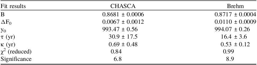
The fitting procedure was carried out using the measured F14C values rather than Δ14C. Because Δ14C is defined as a deviation from the normalized value (∆14C = F14C·exp(ln(2)/5730*(1950-year))–1, expressed in ‰), it is not suitable for the mathematical treatment required here. The best-fit results (Table 1, Figure 8) indicate that the amplitude of the excess is about 30% smaller in CHASCA than in the Brehm series, while the decay constants are compatible within uncertainties, although the dispersion of the CHASCA data degrades the estimate. The step values in Δ14C are 7.5‰ and 12.4‰, respectively. The timing of the signal points to an excess in mid-993 in the Southern Hemisphere and early-994 in the Northern Hemisphere. The indicative significance is computed from the difference between the background and the sum of the background and jump levels (δB and δΔF0 are the errors on B and F0 respectively):
 $\sigma = \;{{\left( {B + \Delta {{\rm{F}}_0}} \right) - B} \over {\sqrt {{{\left( {\delta B + \delta \Delta {F_0}} \right)}^2} + \delta {B^2}\;} }}$
Best-fit parameters for the CHASCA and Brehm datasets around the AD 993–994 excess, using the F14C data. The parameters consist of the background level (B), the jump amplitude (ΔF0), the onset year (y0), the decay constant (τ), and the time resolution factor (κ). The quality of the fit is measured with the reduced χ2 and the significance quantifies the signal excess over the initial assumed background.

Table 1 Long description
A table comparing fit results for CHASCA and Brehm datasets. The table has 8 rows and 3 columns. The columns are labeled 'Fit results', 'CHASCA', and 'Brehm'. The rows are labeled with different parameters: B, ΔF0, y0, τ (yr), κ (yr), χ² (reduced), and Significance. Each cell contains a value with its uncertainty. Row 1: B, 0.8681 ± 0.0006, 0.8717 ± 0.0004. Row 2: ΔF0, 0.0067 ± 0.0012, 0.0110 ± 0.0009. Row 3: y0, 993.47 ± 0.56, 994.07 ± 0.26. Row 4: τ (yr), 30.9 ± 17.5, 16.4 ± 3.6. Row 5: κ (yr), 0.69 ± 0.48, 0.53 ± 0.12. Row 6: χ² (reduced), 0.84, 0.99. Row 7: Significance, 6.8, 8.9.
The signal significance exceeds 7 σ for CHASCA data and 9 σ for Brehm series.
The CHASCA signal provides clear evidence of the AD 993–994 event in South America, in good agreement with Northern Hemisphere records.
4. Comparison with the Southern Hemisphere series
In the Southern Hemisphere, only a few radiocarbon series are available, and even fewer at annual resolution. For the period covered by CHASCA, only two other series exist : Dargaville, New Zealand (35.92 ºS, 173.80 ºE; Agathis australis) and El Asiento, Chile (32.65 ºS, 70.82 ºW; Austrocedrus chilensis) (Büntgen et al. Reference Büntgen, Wacker, Galván, Arnold, Arseneault, Baillie, Beer, Bernabei, Bleicher, Boswijk, Bräuning, Carrer, Ljungqvist, Cherubini, Christl, Christie, Clark, Cook, D’Arrigo, Davi, Eggertsson, Esper, Fowler, Gedalof, Gennaretti, Grießinger, Grissino-Mayer, Grudd, Gunnarson, Hantemirov, Herzig, Hessl, Heussner, Jull, Kukarskih, Kirdyanov, Kolář, Krusic, Kyncl, Lara, LeQuesne, Linderholm, Loader, Luckman, Miyake, Myglan, Nicolussi, Oppenheimer, Palmer, Panyushkina, Pederson, Rybníček, Schweingruber, Seim, Sigl, Churakova (Sidorova), Speer, Synal, Tegel, Treydte, Villalba, Wiles, Wilson, Winship, Wunder, Yang and Young2018), both spanning AD 990–1000. Originally published by Büntgen et al. (Reference Büntgen, Wacker, Galván, Arnold, Arseneault, Baillie, Beer, Bernabei, Bleicher, Boswijk, Bräuning, Carrer, Ljungqvist, Cherubini, Christl, Christie, Clark, Cook, D’Arrigo, Davi, Eggertsson, Esper, Fowler, Gedalof, Gennaretti, Grießinger, Grissino-Mayer, Grudd, Gunnarson, Hantemirov, Herzig, Hessl, Heussner, Jull, Kukarskih, Kirdyanov, Kolář, Krusic, Kyncl, Lara, LeQuesne, Linderholm, Loader, Luckman, Miyake, Myglan, Nicolussi, Oppenheimer, Palmer, Panyushkina, Pederson, Rybníček, Schweingruber, Seim, Sigl, Churakova (Sidorova), Speer, Synal, Tegel, Treydte, Villalba, Wiles, Wilson, Winship, Wunder, Yang and Young2018), the Dargaville series was later complemented with additional duplicates before being incorporated into SHCal20 (Figure 1b in Hogg et al. Reference Hogg, Heaton, Hua, Palmer, Turney, Southon, Bayliss, Blackwell, Boswijk, Bronk Ramsey, Pearson, Petchey, Reimer, Reimer and Wacker2020). The two published series being only 10 rings long, a step-plus-decay fit cannot be applied to either of them, and the comparison is therefore limited to a visual assessment (Figure 4b).
Three striking features emerge from our results. First, the CHASCA series shows an overall structure similar to SHCal20, yet it frequently shows lower F14C values (74 out of 115 rings), indicating a systematic trend toward slightly reduced 14C levels in Patagonia, Argentina (Figure 4c). Second, CHASCA clearly captures the AD 993–994 event, but the amplitude of the peak is markedly less than in Dargaville, New Zealand, and El Asiento, Chile. Third, although CHASCA and SHCal20 share similar trends, individual features vary in expression, with some being attenuated and others accentuated.
These observations collectively suggest that local or regional factors may influence the CHASCA record, affecting both the F14C background levels and the expression of short-term events such as the AD 993-994 SPE. The differences may arise from terrestrial factors, acting individually or in combination, that affect the production, transport, and recording of cosmogenic 14C, including the geomagnetic field (particularly the South Atlantic Anomaly), stratosphere–troposphere exchanges, oceanic upwelling, and tree phenology.
4.1 Geomagnetic modulation
The production of cosmogenic isotopes is significantly modulated by large non-dipole components of the geomagnetic field. The mid-latitudes of South America are today under the influence of the South Atlantic Anomaly (SAA), a large non-dipole feature generated by reversed flux patches at the Earth’s core surface (e.g., Terra-Nova et al. Reference Terra-Nova, Amit, Hartmann, Trindade and Pinheiro2017), and possibly linked to heterogeneities in the lowermost mantle (Tarduno et al. Reference Tarduno, Watkeys, Huffman, Cottrell, Blackman, Wendt, Scribner and Wagner2015). By weakening geomagnetic shielding, this anomaly allows enhanced penetration of galactic cosmic rays into the atmosphere (Heirtzler, Reference Heirtzler2002). Had this configuration been active around 1000 AD, it would have favored higher cosmogenic production in South America relative to New Zealand. The SAA is well documented for the last four centuries, with evidence of a westward drift (e.g., Schanner et al. Reference Schanner, Bohsung, Fischer, Korte and Holschneider2023), but paleomagnetic records around AD 1000 remain sparse and partly contradictory: archeomagnetic data from baked clays in Argentina and Brazil suggest that field intensity was nearly twice its modern value (Goguitchaichvili et al. Reference Goguitchaichvili, García-Ruiz, Greco, Kravchinsky, Rodríguez, Morales and Berkovich2023; Gómez-Paccard et al. Reference Gómez-Paccard, Chauvin, Albeck, Zaburlín, Basso, Pavón-Carrasco, Osete and Campuzano2019; Poletti et al. Reference Poletti, Trindade, Hartmann, Damiani and Rech2016). Between AD 800 and AD 1100, the secular variation appeared rapid at the multidecadal scale in potteries from Argentina (Gómez-Paccard et al. Reference Gómez-Paccard, Bonilla-Alba and Mallea2025), whereas stalagmite records from Brazil point instead to a decline in geomagnetic strength (Trindade et al. Reference Trindade, Jaqueto, Terra-Nova, Brandt, Hartmann, Feinberg, Strauss, Novello, Cruz, Karmann, Cheng and Edwards2018). This uncertainty prevents firm conclusions, but geomagnetic modulation can be considered as a potential contributor to regional contrast in 14C production. However, while geomagnetic effects influence long-term production rates, they cannot fully account for the reduced amplitude of the AD 993 peak in CHASCA, since baseline F14C levels at the three sites start at roughly comparable values. They might instead play a role in the higher baseline around AD 775 in Patagonia compared with records in New Zealand and Australia (Hogg et al. Reference Hogg, Heaton, Hua, Palmer, Turney, Southon, Bayliss, Blackwell, Boswijk, Bronk Ramsey, Pearson, Petchey, Reimer, Reimer and Wacker2020—Figure 1).
4.2 Atmospheric transport
Model simulations (Golubenko et al. Reference Golubenko, Rozanov, Kovaltsov and Usoskin2022) reveal that 14C production and transport are not only modulated by the mean altitude of the tropopause but also by its temporal fluctuations, both tied to tropospheric circulation dynamics. The latitude band around 30–40º is particularly sensitive to the variability in stratosphere–troposphere exchange. Located near the subtropical boundary (∼30 ºS), the transition band between the descending branches of the Hadley and Ferrel cells (Hu and Fu Reference Hu and Fu2007), Dargaville (35.9 ºS) and El Asiento (32.6 ºS) are subjected to strong frontal activity, tropopause folds, and Rossby-Wave breaking, which frequently inject stratospheric air into the lower troposphere (Figure 1). These dynamical features may have enhanced the downward flux of newly produced 14C following the AD 993 SPE. In contrast, CHASCA (42.7 ºS) lies further poleward, in the core mid-latitudes, where more persistent stratification and blocking may tend to limit the occurrence of rapid descent events. Thus, even with similar stratospheric production, latitude-dependent transport dynamics may have influenced how much and when “fresh” 14C reached the surface atmosphere during the tree growing season. This mechanism may explain why the proportion of fresh 14C was lower at CHASCA than at Dargaville and El Asiento, producing regional differences in the recorded signal.
4.3 Ocean–atmosphere exchanges
Ocean–atmosphere interactions may have also contributed to the observed differences. Independent ∆14CO2 records show systematically lower values at Campbell Island (New Zealand) compared with Chilean sites at similar latitudes (Lewis et al. Reference Lewis, Corran, Mikaloff-Fletcher, Behrens, Moss, Brailsford, Lorrey, Norris and Turnbull2025), a contrast that has been attributed to Southern Ocean upwelling that injects 14C-depleted CO2 into the atmosphere, diluting the cosmogenic 14C signal in New Zealand. Such dilution would be expected to dampen the cosmogenic signal over New Zealand whereas South American sites are less affected. Along the Pacific coast of South America, upwelling zones off Chile and Peru (e.g. the Humboldt Current system, Montecino and Lange (Reference Montecino and Lange2009)—see Figure 1) are well documented to bring up deep, old 14C-poor waters, thereby increasing the marine reservoir age and affecting local air–sea CO2 exchange (Carré et al. Reference Carré, Jackson, Maldonado, Chase and Sachs2017). These marine-derived CO2 inputs could dampen or dilute atmospheric 14C signals above adjacent land areas. El Asiento, being closer to such coastal upwelling zones, may receive more of this effect than CHASCA, which is located further inland and poleward. However, there is no current evidence that upwelling zones extended substantially southward into CHASCA’s latitude (∼42.7 ºS) around AD 993. Furthermore, a southward expansion of upwelling would likely have been associated with higher regional precipitation or other climate shifts detectable in paleoclimate proxies; such signals are not clearly observed (e.g., Lara et al. Reference Lara, Villalba, Urrutia-Jalabert, González-Reyes, Aravena, Luckman, Cuq, Rodríguez and Wolodarsky-Franke2020). A more local possibility could involve microclimatic influences: soil respiration, lake CO2 fluxes, or local vegetation effects could change atmospheric CO2 composition locally. If such CO2 were depleted in 14C (e.g. from old soil carbon), it could reduce the amplitude of an atmospheric 14C spike recorded by trees. However, if these effects were substantial, one might expect correlated shifts in δ13C, which are not evident in our data.
4.4 Tree physiology
Biological factors must be considered, as tree species differ in the length and timing of their cambial reactivation, which determines which portion of the annual atmospheric 14C signal is incorporated into tree ring. Fitzroya cupressoides, used in the Argentine record, has a relatively narrow cambial growth season, typically restricted to austral late spring–summer (mid October to mid-February), after which xylem formation rapidly declines (Figure 3). Although cambial phenology was not measured directly at El Asiento, dendroclimatological studies on Austrocedrus chilensis indicate that radial growth is largely concentrated in late calendar year, during austral spring and early summer (approximately September to December, occasionally extending into January) (Le Quesne et al. Reference Le Quesne, Stahle, Cleaveland, Therrell and Aravena2006). This implies that A. chilensis resumes cambial activity earlier in spring than Fitzroya, creating a period during wich A. chilensis is already forming xylem while Fitzroya remains dormant. By contrast, Agathis australis (kauri, New Zealand) can grow from early spring until late autumn, sometimes extending to April or May under favourable conditions (Odgen Reference Odgen1983). Kauri therefore integrates a longer portion of the annual atmospheric 14C signal.
Because intra-hemispheric redistribution of 14C likely occurs on seasonal timescales, differences in spike amplitude are likely to reflect species-specific growth timing. Species with longer or earlier growing seasons may therefore integrate a larger fraction of the anomaly, whereas shorter or later growth periods could yield reduced amplitudes.
5. Conclusion
Our study provides the first multi-decadal annually resolved radiocarbon record from South America, spanning from AD 970 to 1084, and securely anchored by dendrochronology of Fitzroya cupressoides. The CHASCA series demonstrates overall consistency with the Brehm et al. (Reference Brehm, Bayliss, Christl, Synal, Adolphi, Beer, Kromer, Muscheler, Solanki, Usoskin, Bleicher, Bollhalder, Tyers and Wacker2021) Northern Hemisphere datasets and with SHCal20, with a confirmation of the expected interhemispheric offset. Importantly, it captures the AD 993–994 solar particle event with a 7 σ significance, though with a weaker amplitude than decade-long series available in New Zealand and Chile. This attenuation likely reflects a combination of regional environmental conditions and species-specific growth dynamics, underscoring the complexity of local expressions of cosmogenic 14C signals. CHASCA thus positions South America as a key region for detecting and comparing short-term cosmogenic 14C events.
Supplementary material
To view supplementary material for this article, please visit https://doi.org/10.1017/RDC.2026.10233
Acknowledgments
This project was supported by the CNRS Interdisciplinary Mission (MITI) through the TEMPS call (project CHASCA), and by the CEA, which funded KL’s PhD scholarship. We thank Yoann Roy (Menuiserie Roy, Gif-sur-Yvette) for providing radial segments from the original trunk cross-section used in this study.
Competitive interest
The authors declare no competitive interest.