1 Legacy software packages for dense linear algebra
Over the years, computational physics and chemistry have provided ongoing demand for the ever-increasing performance in hardware and software required to efficiently solve problems in these fields. Fortunately, most of these problems can be translated into solutions for systems of linear equations – the very topic of numerical linear algebra. Seemingly then, a set of efficient linear solvers could be solving important scientific problems for years to come. We also argue that dramatic changes in hardware design, precipitated by the shifting nature of the computer hardware marketplace, has had a continuous effect on numerical linear algebra software, and the extraction of high percentages of peak performance from evolving hardware requires continuous adaptation in software. If the history of linear algebra software’s adaptive nature is any indication, then the future holds yet more changes – changes aimed at harnessing the incredible advances of the evolving hardware infrastructure.
1.1 The LINPACK library and its implementations
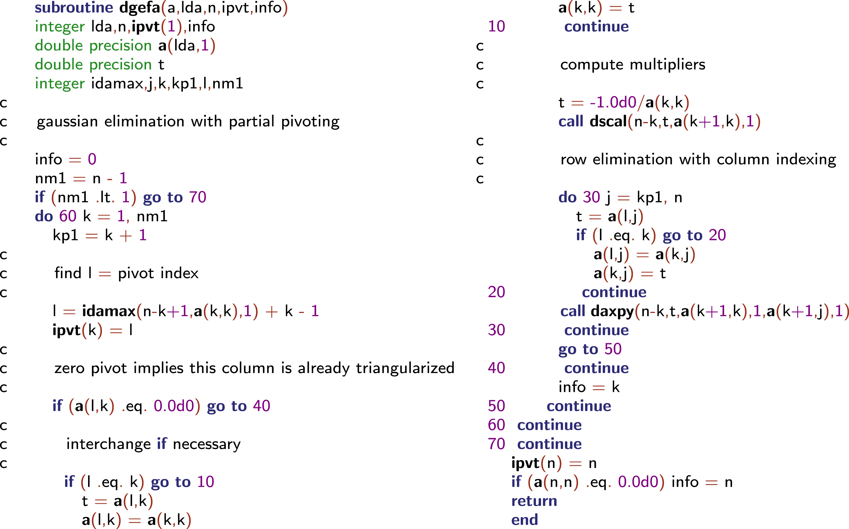
LINPACK variant of LU factorization. This is the original FORTRAN 66 code; if LINPACK were written today it would use a modern Fortran standard.

In the 1970s, Fortran was the language for scientific computation: see Figure 1.1. Fortran stores two-dimensional arrays in column-major order (all of the elements of the first column are stored first, then the elements of the second column are stored, and so on). Accessing the array in a row-wise fashion within the matrix could involve successive memory reference to locations separated from each other by a large increment, depending on the size of the declared array. This situation was further complicated by the operating system’s use of memory pages to effectively control memory usage. With a large matrix and a row-oriented algorithm in a Fortran environment, an excessive number of page swaps might be generated in the process of running the software. Cleve Moler pointed out this issue in the 1970s (Moler Reference Moler1972).
In the mid-to-late 1970s, the introduction of vector computer systems marked the beginning of modern supercomputing. These systems offered a performance advantage of at least one order of magnitude over conventional systems of that time. Raw performance was the main, if not the only, selling point of new computing hardware. In the first half of the 1980s the integration of vector systems in conventional computing environments became more important. Only the manufacturers who provided standard programming environments, operating systems, and key applications were successful in earning industrial customers and survived. Performance was mainly increased by improved chip technologies and by producing shared memory multiprocessor systems. These systems were able, in one step, to perform a single operation on a relatively large number of operands stored in vector registers. Expressing matrix algorithms as vector–vector operations was a natural fit for this type of machine (Dongarra, Gustavson and Karp Reference Dongarra, Gustavson and Karp1984). However, some of the vector designs had a limited ability to load and store the vector registers in main memory. A technique called ‘chaining’ allowed this limitation to be circumvented by moving data between the registers before accessing main memory. Chaining required recasting linear algebra in terms of matrix–vector operations.
Vector architectures exploit pipeline processing by running mathematical operations on arrays of data in a simultaneous or pipelined fashion. Most algorithms in linear algebra can be easily vectorized. Therefore, in the late 1970s there was an effort to standardize vector operations for use in scientific computations. The idea was to define some simple, frequently used operations and implement them on various systems to achieve portability and efficiency. This package came to be known as the Level 1 Basic Linear Algebra Subprograms (BLAS) or Level 1 BLAS (Lawson, Hanson, Kincaid and Krogh Reference Lawson, Hanson, Kincaid and Krogh1979).
The term Level 1 denotes vector–vector operations. As we will see, Level 2 (matrix–vector operations: Hammarling, Dongarra, Du Croz and Hanson Reference Hammarling, Dongarra, Du Croz and Hanson1988), and Level 3 (matrix–matrix operations: Dongarra, Du Croz, Hammarling and Duff Reference Dongarra, Du Croz, Hammarling and Duff1990) play important roles as well. In the 1970s, dense linear algebra algorithms were implemented in a systematic way by the LINPACK project (Dongarra, Bunch, Moler and Stewart Reference Dongarra, Bunch, Moler and Stewart1979). LINPACK is a collection of Fortran subroutines that analyse and solve linear equations and linear least-squares problems. The package solves linear systems whose matrices are general, banded, symmetric indefinite, symmetric positive definite, triangular, and square tridiagonal (only diagonal, super-diagonal, and sub-diagonal are present). In addition, the package computes the QR (matrix Q is unitary or Hermitian and R is upper trapezoidal) and singular value decompositions of rectangular matrices and applies them to least-squares problems. LINPACK uses column-oriented algorithms, which increase efficiency by preserving locality of reference. By column orientation, we mean that the LINPACK code always references arrays down columns, not across rows. This is important since Fortran stores arrays in column-major order. This means that as one proceeds down a column of an array, the memory references proceed sequentially through memory. Thus, if a program references an item in a particular block, the next reference is likely to be in the same block.
The software in LINPACK was kept machine-independent partly through the introduction of the Level 1 BLAS routines. Calling Level 1 BLAS did almost all of the computation. For each machine, the set of Level 1 BLAS would be implemented in a machine-specific manner to obtain high performance. The Level 1 BLAS subroutines DAXPY, DSCAL, and IDAMAX are used in the routine DGEFA.
It was presumed that the BLAS operations would be implemented in an efficient, machine-specific way suitable for the computer on which the subroutines were executed. On a vector computer, this could translate into a simple, single vector operation. This avoided leaving the optimization up to the compiler and explicitly exposing a performance-critical operation.
In a sense, then, the beauty of the original code was regained with the use of a new vocabulary to describe the algorithms: the BLAS. Over time, the BLAS became a widely adopted standard and was most likely the first to enforce two key aspects of software: modularity and portability. Again, these are taken for granted today, but at the time they were not. One could have the advantages of the compact algorithm representation and the portability, because the resulting Fortran code was portable.
Most algorithms in linear algebra can be easily vectorized. However, to gain the most out of such architectures, simple vectorization is usually not enough. Some vector computers are limited by having only one path between memory and the vector registers. This creates a bottleneck if a program loads a vector from memory, performs some arithmetic operations, and then stores the results. In order to achieve top performance, the scope of the vectorization must be expanded to facilitate chaining operations together and to minimize data movement, in addition to using vector operations. Recasting the algorithms in terms of matrix–vector operations makes it easy for a vectorizing compiler to achieve these goals.
Thus, as computer architectures became more complex in the design of their memory hierarchies, it became necessary to increase the scope of the BLAS routines from Level 1 to Level 2 to Level 3.
1.2 Implementation in terms of submatrices
RISC (reduced instruction set computing) computers were introduced in the late 1980s and early 1990s. While their clock rates might have been comparable to those of the vector machines, the computing speed lagged behind due to their lack of vector registers. Another deficiency was their creation of a deep memory hierarchy with multiple levels of cache memory to alleviate the scarcity of bandwidth that was, in turn, caused mostly by a limited number of memory banks. The eventual success of this architecture is commonly attributed to the price point and astonishing improvements in performance over time as predicted by Moore’s law (Moore Reference Moore1965). With RISC computers, the linear algebra algorithms had to be redone yet again. This time, the formulations had to expose as many matrix–matrix operations as possible, which guaranteed good cache re-use.
As mentioned before, the introduction in the late 1970s and early 1980s of vector machines brought about the development of another variant of algorithms for dense linear algebra. This variant was centred on the multiplication of a matrix by a vector. These subroutines were meant to give improved performance over the dense linear algebra subroutines in LINPACK, which were based on Level 1 BLAS. In the late 1980s and early 1990s, with the introduction of RISC-type microprocessors (the ‘killer micros’) and other machines with cache-type memories, we saw the development of LAPACK (Anderson et al. Reference Anderson, Bai, Bischof, Blackford, Demmel, Dongarra, Ducroz, Greenbaum, Hammarling, McKenney and Sorensen1999) Level 3 algorithms for dense linear algebra. A Level 3 code is typified by the main Level 3 BLAS, which, in this case, is matrix multiplication (Anderson and Dongarra Reference Anderson and Dongarra1990b).
The original goal of the LAPACK project was to allow linear algebra problems to run efficiently on vector and shared memory parallel processors. On these machines, LINPACK is inefficient because its memory access patterns disregard the multilayered memory hierarchies of the machines, thereby spending too much time moving data instead of doing useful floating-point operations. LAPACK addresses this problem by reorganizing the algorithms to use block matrix operations, such as matrix multiplication, in the innermost loops (see the paper by Anderson and Dongarra Reference Anderson and Dongarra1990a). These block operations can be optimized for each architecture to account for its memory hierarchy, and so provide a transportable way to achieve high efficiency on diverse modern machines.
Here we use the term ‘transportable’ instead of ‘portable’ because, for fastest possible performance, LAPACK requires that highly optimized block matrix operations already be implemented on each machine. In other words, the correctness of the code is portable, but high performance is not – if we limit ourselves to a single Fortran source code.
LAPACK can be regarded as a successor to LINPACK in terms of functionality, although it does not use the same function-calling sequences. As such a successor, LAPACK was a win for the scientific community because it could keep LINPACK’s functionality while getting improved use out of new hardware.
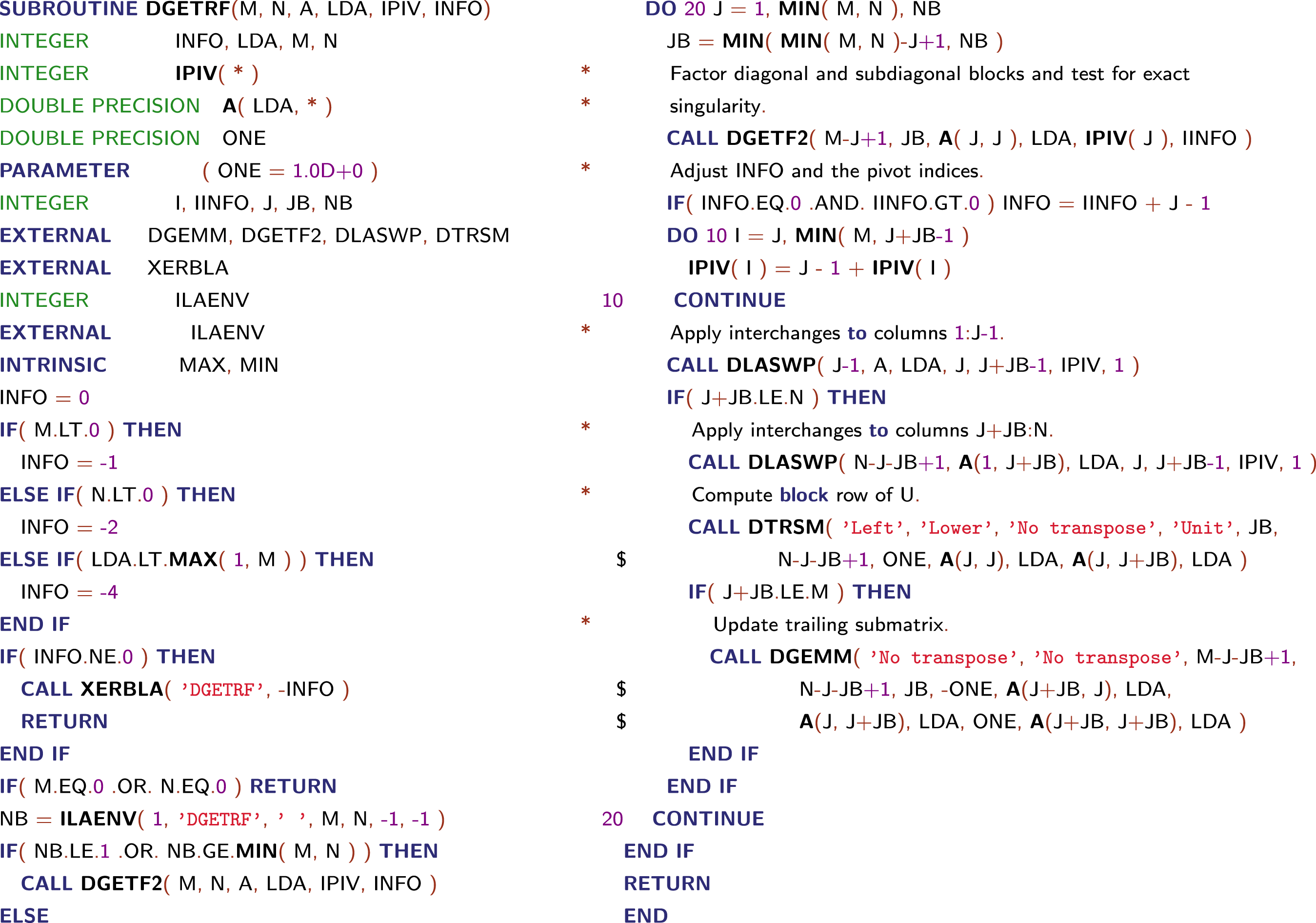
LAPACK’s LU factorization routine DGETRF using FORTRAN 77.
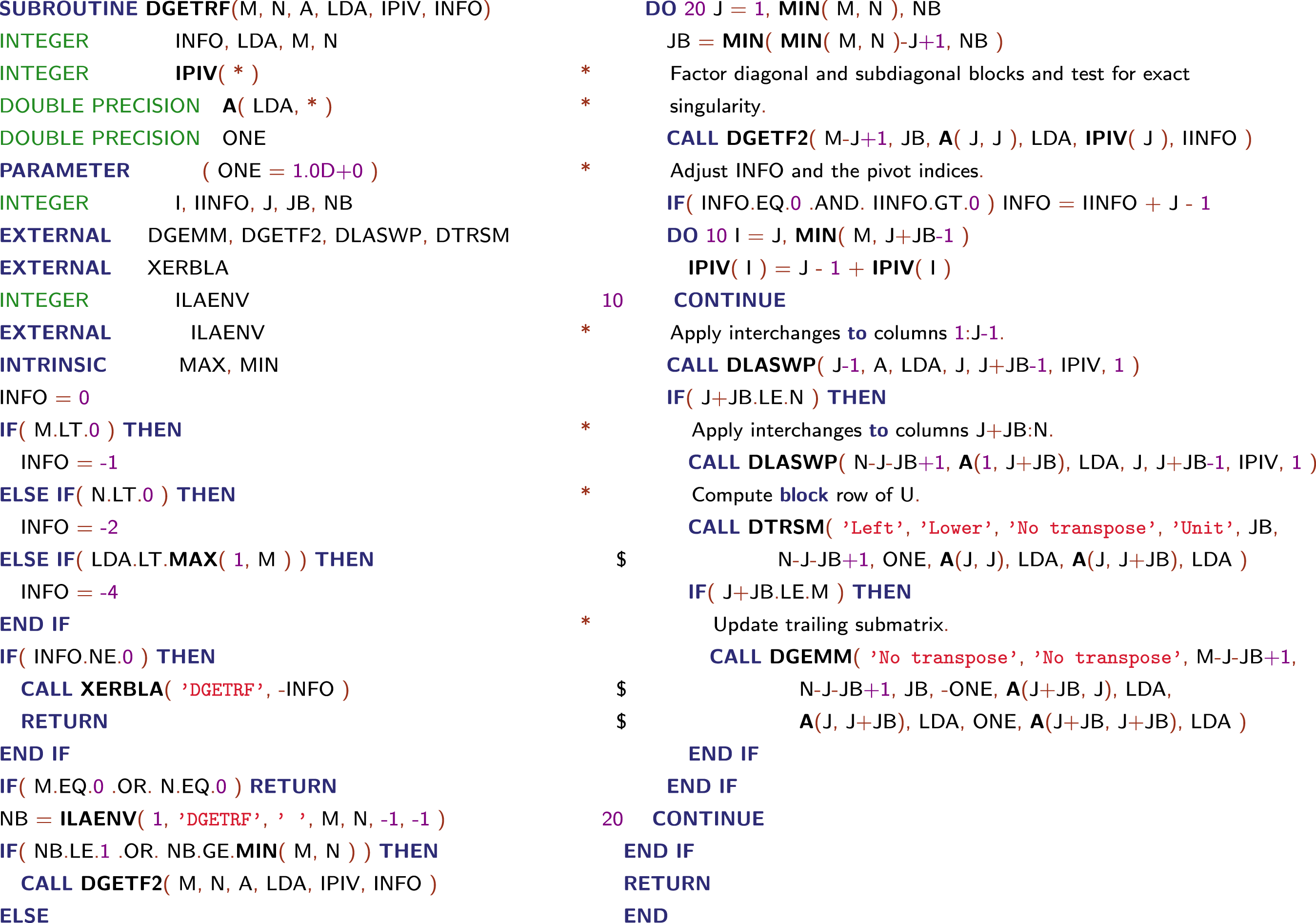
Most of the computational work in the algorithm from Figure 1.2 is contained in three routines:
∙ DGEMM – matrix–matrix multiplication,
∙ DTRSM – triangular solve with multiple right-hand sides,
∙ DGETF2 – unblocked LU factorization for operations within a block column.
One of the key parameters in the algorithm is the block size, called NB here. If NB is too small or too large, poor performance can result – hence the importance of the ILAENV function, whose standard implementation was meant to be replaced by a vendor implementation encapsulating machine-specific parameters upon installation of the LAPACK library. At any given point of the algorithm, NB columns or rows are exposed to a well-optimized Level 3 BLAS. If NB is 1, the algorithm is equivalent in performance and memory access patterns to LINPACK’s version.
Matrix–matrix operations offer the proper level of modularity for performance and transportability across a wide range of computer architectures, including parallel systems with memory hierarchy. This enhanced performance is due primarily to a greater opportunity for re-using data. There are numerous ways to accomplish this re-use of data to reduce memory traffic and to increase the ratio of floating-point operations to data movement through the memory hierarchy. This improvement can bring a three- to tenfold improvement in performance on modern computer architectures.
The jury is still out concerning the productivity of writing and reading the LAPACK code: How hard is it to generate the code from its mathematical description? The use of vector notation in LINPACK is arguably more natural than LAPACK’s matrix formulation. The mathematical formulas that describe algorithms are usually more complex if only matrices are used, as opposed to mixed vector–matrix notation.
1.3 Beyond a single compute node
The traditional design focus for massively parallel processing (MPP) systems was the very high end of performance. In the early 1990s, the symmetric multiprocessing (SMP) systems of various workstation manufacturers, as well as the IBM SP series – which targeted the lower and medium market segments – gained great popularity. Their price/performance ratios were better thanks to the economies of scale associated with larger production numbers, and due to lack of overhead in the design for support of the very large configurations. Due to the vertical integration of performance, it was no longer economically feasible to produce and focus on the highest end of computing power alone. The design focus for new systems shifted to the market of medium performance systems.
The acceptance of MPP systems, not only for engineering applications but also for new commercial applications (e.g. databases), emphasized different criteria for market success, such as the stability of the system, continuity/longevity of the manufacturer, and price/performance. Thriving in commercial environments became an important endeavour for a successful supercomputer business in the late 1990s. Due to these factors, and the consolidation of the number of vendors in the market, hierarchical systems built with components designed for the broader commercial market replaced homogeneous systems at the very high end of performance. The marketplace adopted clusters of SMPs readily, while academic research focused on clusters of workstations and PCs.
At the end of the 1990s, clusters were common in academia but mostly as research objects and not primarily as general-purpose computing platforms for applications. Most of these clusters were of comparable small scale, and as a result the November 1999 edition of the TOP500 (Meuer, Strohmaier, Dongarra and Simon Reference Meuer, Strohmaier, Dongarra and Simon2011) listed only seven cluster systems. This changed dramatically as industrial and commercial customers started deploying clusters as soon as applications with less stringent communication requirements permitted them to take advantage of the better price/performance ratio. At the same time, all major vendors in the HPC market started selling this type of cluster to their customer base. In November 2004, clusters were the dominant architectures in the TOP500, with 294 systems at all levels of performance. Companies such as IBM and Hewlett-Packard were selling the majority of these clusters, and a large number of them were installed for commercial and industrial customers.
In the early 2000s, clusters built with off-the-shelf components gained more and more attention not only as academic research objects, but also as viable computing platforms for end-users of HPC computing systems. By 2004, these groups of clusters represented the majority of new systems on the TOP500 in a broad range of application areas. One major consequence of this trend was the rapid rise in the utilization of Intel processors in HPC systems. While virtually absent in the high end at the beginning of the decade, Intel processors are now used in the majority of HPC systems. Clusters in the 1990s were mostly self-made systems designed and built by small groups of dedicated scientists or application experts. This changed rapidly as soon as the market for clusters based on PC technology matured. Today, the large majority of TOP500-class clusters are manufactured and integrated by either a few traditional large HPC manufacturers, such as IBM or Hewlett-Packard, or numerous small, specialized integrators of such systems.
In addition, clusters generally still have different uses compared to their more integrated counterparts: clusters are mostly used for capacity computing, while the integrated machines are primarily used for capability computing. The largest supercomputers are used for capability or turnaround computing where the maximum processing power is applied to a single problem. The goal is to solve a larger problem, or to solve a single problem in a shorter period of time. Capability computing enables the solution of problems that cannot otherwise be solved in a reasonable period of time (e.g., by moving from a two-dimensional to a three-dimensional simulation, using finer grids, or using more realistic models). Capability computing also enables the solution of problems with real-time constraints (e.g. predicting weather). The main figure of merit is time to solution. Smaller or cheaper systems are used for capacity computing, where smaller problems are solved. Capacity computing can be used to enable parametric studies or to explore design alternatives; it is often needed to prepare for more expensive runs on capability systems. Capacity systems will often run several jobs simultaneously. The main figure of merit is sustained performance per unit cost. Traditionally, vendors of large supercomputer systems have learned to provide for the capacity mode of operation as the precious resources of their systems were required to be used as effectively as possible. In contrast, Beowulf clusters (clusters made up of commodity computers linked together via a local area network) mostly use the Linux operating system (a small minority use Microsoft Windows), and these operating systems either lack the tools or the tools lack the maturity to utilize a cluster effectively for capability computing. However, as clusters become both larger and more stable on average, in terms of continuous operation, there is a trend to also use them as computational capability servers.
There are a number of communication networks available for use in clusters. Of course 100 Mb/s Ethernet or Gigabit Ethernet is always possible, which is attractive for economic reasons, but it has the drawback of a high latency ( ${\sim}100~{\rm\mu}\text{s}$) – the time it takes to send the shortest message. Alternatively, there are, for instance, networks that operate from user space, like InfiniBand. The speeds of these networks are more-or-less on a par with some integrated parallel systems. So, apart from the speed of the processors and of the software that is provided by the vendors of traditional integrated supercomputers, the distinction between clusters and the class of custom capability machines becomes rather small and will, especially with advances of the Ethernet standard into the 100 Gb/s territory with latencies well below
 $10~{\rm\mu}\text{s}$, decrease further in the coming years.
LAPACK was designed to be highly efficient on vector processors, high-performance ‘superscalar’ workstations, and shared memory multiprocessors. LAPACK can also be used satisfactorily on all types of scalar machines (PCs, workstations, and mainframes). However, LAPACK in its present form is less likely to give good performance on other types of parallel architectures (e.g. massively parallel single instruction multiple data (SIMD) machines or multiple instruction multiple data (MIMD) distributed memory machines). Instead, the ScaLAPACK effort was intended to adapt LAPACK to these new architectures.
Like LAPACK, the ScaLAPACK routines are based on block-partitioned algorithms in order to minimize the frequency of data movement between different levels of the memory hierarchy. The fundamental building blocks of the ScaLAPACK library are distributed memory versions of the Level 2 and Level 3 BLAS (Choi Reference Choi1995), and a set of Basic Linear Algebra Communication Subprograms (BLACS: Dongarra and Whaley Reference Dongarra and Whaley1995) for communication tasks that arise frequently in parallel linear algebra computations. In the ScaLAPACK routines, all interprocessor communication occurs within the distributed BLAS and the BLACS, so the source code of the top software layer of ScaLAPACK looks very similar to that of LAPACK.
In order to simplify the design of ScaLAPACK, and because the BLAS routines have proved to be very useful tools outside LAPACK, we chose to build a parallel BLAS, or PBLAS (Choi Reference Choi1995), whose interface is as similar to the BLAS as possible. This decision has permitted the ScaLAPACK code to be quite similar, and sometimes nearly identical, to the analogous LAPACK code.
It was our aim that the PBLAS would provide a distributed memory standard, just as the BLAS provided a shared memory standard. This would simplify and encourage the development of high performance and portable parallel numerical software, as well as provide manufacturers with only a small set of routines to be optimized. The acceptance of the PBLAS requires reasonable compromises between competing goals of functionality and simplicity.
The PBLAS operate on matrices distributed in a two-dimensional block cyclic layout. Because such a data layout requires many parameters to fully describe the distributed matrix, we have chosen a more object-oriented approach and encapsulated these parameters in an integer array called an ‘array descriptor’.
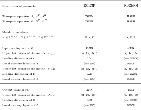
Comparison between parameters of DGEMM and PDGEMM.

By using this descriptor, a call to a PBLAS routine is very similar to a call to the corresponding BLAS routine, as shown in Table 1.1. DGEMM computes C $=$BETA
 $\times$C
 $+$ALPHA
 $\times$op( A )
 $\times$op( B ), where op(A) is either A or its transpose depending on TRANSA, op(B) is similar, op(A) is M
 $\times$K, and op(B) is K
 $\times$N. PDGEMM is the same, with the exception of the way submatrices are specified. To pass the submatrix starting at A(IA,JA) to DGEMM, for example, the actual argument corresponding to the formal argument A is simply A(IA,JA). PDGEMM, on the other hand, needs to understand the global storage scheme of A to extract the correct submatrix, so IA and JA must be passed in separately.
1.4 Into the modern era of heterogeneous hardware
Clearly, the previous sections were historical in nature. Interestingly, many of the design principles and implementation techniques remain relevant when moving into the era of heterogeneous hardware, which requires unprecedented parallelism and customization of algorithmic choices that play into the particular strengths of the underlying computing hardware. The data locality is still important, especially with the growing disparity between the compute units and the memory hierarchy. Vectorization is still present in the form of short vector instructions such as the SSE, AVX, and AltiVec extensions, as well as warps and half-warps on NVIDIA GPUs. Data distribution comes to the fore when deciding the placement of inputs and outputs of the computational kernels, and now includes the decision of dividing the data between the CPU memory and the accelerator memory. Looking back at the past hardware helps one understand these techniques in a much simpler context.
2 New hardware architectures
2.1 The CORAL machines
Current trends in HPC architectures can best be illustrated by the US Department of Energy’s plans for pre-exascale machines, that is, machines with computing capabilities in the range of hundreds of Petaflops, meant to be the stepping stones towards future exascale machines. Under the CORAL collaboration, Oak Ridge National Laboratory (ORNL), Argonne National Laboratory (ANL), and Lawrence Livermore National Laboratory (LLNL) will each deploy powerful pre-exascale supercomputers. These systems will provide the computing power required to meet the mission of the Office of Science and the National Nuclear Security Administration (NNSA) of the US DoE. While NVIDIA GPU-accelerated systems, named Summit and Sierra and based on the IBM OpenPOWER platform, were selected for ORNL and LLNL, an Intel system named Aurora and based on the Xeon Phi platform was selected for ANL. These systems will serve as the models for future exascale designs.
The NVIDIA/IBM-based systems will share a heterogeneous node architecture that tightly integrates IBM POWER CPUs with NVIDIA GPUs using NVIDIA NVLink high-speed coherent interconnect technology. Both machines will be based on IBM Power9 chips, which will emerge just in time for delivery of these systems. The performance and efficiency boost will come from NVIDIA Volta Tesla GPUs, with Mellanox EDR InfiniBand hooking the hybrid Power-Tesla nodes together. The two key features of the Volta GPU are the stacked memory and NVLink interconnect, both of which are important for keeping the processors on both the Power and Tesla components fed. At the same time, the Aurora system at ANL will rely on Intel’s HPC scalable system framework, which is a flexible blueprint for developing high-performance, balanced, power-efficient, and reliable systems capable of supporting both compute- and data-intensive workloads. The framework combines next generation Intel Xeon processors and Intel Xeon Phi processors, Intel Omni-Path fabric, silicon photonics, and innovative memory technologies.
2.2 Stacked memory
3D-stacked memories are manufactured by stacking silicon wafers and/or dies and interconnecting them vertically using through-silicon vias (TSVs), so that they behave as a single device to achieve performance improvements with reduced power consumption and smaller footprint than conventional two-dimensional memory. Two leading three-dimensional memory technologies are high bandwidth memory (HBM) and hybrid memory cube (HMC). HBM is a high-performance RAM interface for 3D-stacked DRAM memory from AMD and Hynix. It is to be used in conjunction with high-performance graphics accelerators and network devices. HBM achieves higher bandwidth while using less power in a substantially smaller form factor than DDR4 or GDDR5. This is achieved by stacking up to eight DRAM dies, including an optional base die with a memory controller, which are interconnected by TSVs and microbumps. The first chip utilizing HBM is AMD Fiji, powering the AMD Radeon R9 Fury X. While the memory bandwidth of the Fury X GPU peaks at 512 GB/s, by 2018 the bandwidth of the NVIDIA Volta is expected to approach 1 TB/s.
HMC is a high-performance RAM interface for TSV-based stacked DRAM memory competing with HBM. HMC promises a  $15\times$ speed improvement from DDR3. HMC is backed by several major technology companies including Samsung, Micron Technology, Open-Silicon, ARM, HP, Microsoft, Altera, and Xilinx. Both Intel and IBM target HMC as the memory technology for their future processors. HMC combines TSVs and microbumps to connect multiple dies of memory cell arrays on top of each other. The memory controller is integrated as a separate die. HMC uses standard DRAM cells but it has more data banks than classic DRAM memory of the same size. HMC is intended to greatly increase the amount of memory bandwidth that can be used to feed a processor. This is accomplished by putting the memory as close to the processor as possible to allow what is essentially an extremely wide memory interface, through which an enormous amount of memory bandwidth can be created. The current standard allows for bandwidths as high as 320 GB/s, while IBM advertises bandwidths as high as 230 GB/s for the Power8 CPU.
Multi-channel DRAM (MCDRAM) is a variant of HMC designed just for Intel’s processors. Intel and Micron have taken HMC and replaced the standard memory interface with a custom interface better suited for the next generation Xeon Phi, the Knights Landing. The end result is a memory technology that can scale up to 16 GB of RAM while offering up to 500 GB/s of memory bandwidth.
2.3 NVLink
NVLink is the node integration interconnect for both the Summit and Sierra pre-exascale supercomputers commissioned by the US Department of Energy, enabling NVIDIA GPUs and CPUs such as IBM POWER to access each other’s memory quickly and seamlessly. NVLink is an energy-efficient, high-bandwidth path between the GPU and the CPU that uses up to  $3\times$ less energy to move data on the node at bandwidths of 80–200 GB/s, or
 $5\times$ to
 $12\times$ that of the current PCIe Gen3 x16, delivering faster application performance. Each compute node in Summit will be equipped with over 512 GB of coherent memory, including large-capacity DDR4 system memory and ultra-fast HBM stacked memory on the GPU. All data will be directly addressable from either the CPU or the GPU, an important feature enabled by the NVLink interconnect.
2.4 Intel Omni-Path and silicon photonics
Intel Omni-Path is Intel’s interconnection technology competing with InfiniBand. While the Summit and Sierra systems will have Mellanox’s EDR 100 Gb/s InfiniBand networks, The Aurora system will have an Omni-Path network. Starting with the Knights Landing processor, and continuing with Knights Hill, Intel will be integrating their fabric controller on to the processor itself, doing away with the external fabric controller, the space it occupies, and the potential bottlenecks that come from using a discrete fabric controller. Current versions of Omni-Path are running at 100 Gb/s, using the Prairie River chip. Before the delivery of the Aurora machine, it is expected to scale up to at least 200 Gb/s, utilize silicon photonics, and be based on the Wolf River chip.
Silicon photonics is an application of photonic systems which use silicon as an optical medium. Silicon photonic devices can be made using existing semiconductor fabrication techniques, and because silicon is already used as the substrate for most integrated circuits, it is possible to create hybrid devices in which the optical and electronic components are integrated onto a single microchip. Consequently, silicon photonics is being actively researched by many electronics manufacturers including Intel and IBM, as well as by academic research groups, and is seen as a means for keeping on track with Moore’s law, by using optical interconnects to provide faster data transfer both between and within microchips.
2.5 Hybrid computing
The Summit and Sierra computers put emphasis on hybrid computing. For uncompromising performance, a heterogeneous architecture, coupling powerful latency-optimized processors with highly parallel throughput-optimized accelerators, can significantly outperform non-specialized, homogeneous alternatives. Today’s most successful scalable HPC applications distribute data, work across the nodes of a system, and organize algorithms to operate as independently as possible on millions or billions of data elements. However, even simple applications can transition many times between periods of throughput-intensive parallel calculations and sections of latency-sensitive serial operations. The architectural emphasis on parallelism in GPUs leads to optimization for throughput, hiding, rather than minimizing, latency. Support for thousands of threads ensures a ready pool of work in the face of data dependencies in order to sustain performance at a high percent of peak. The memory hierarchy design and technology thoroughly reflect optimization for throughput performance at minimal energy per bit. By contrast, a latency-optimized CPU architecture drives completely different design decisions. Techniques designed to compress the execution of a single instruction thread into the smallest possible time demand a host of architectural features (e.g. branch prediction, speculative execution, register renaming) that would cost far too much energy to be replicated for thousands of parallel GPU threads, but are entirely appropriate for CPUs. The essence of the heterogeneous computing model is that one size does not fit all. Parallel and serial segments of the workload execute on the best-suited processor – latency-optimized CPU or throughput-optimized GPU – delivering faster overall performance, greater efficiency, and lower energy and cost per unit of computation.
By contrast, the Aurora computer offers a much more homogeneous environment. While the existing Knights Corner (first generation Xeon Phi) is a slot-in coprocessor, that must be paired with a standard Xeon CPU, the next generation Knights Landing will be a standalone processor (‘self-hosted’), and so will its successor, Knights Hill, which will power the Aurora. Knights Landing will have up to 16 GB of DRAM, 3D-stacked on-package, providing up to 500 GB/s of memory bandwidth (along with up to 384 GB of DDR4-2400 mainboard memory). It also promises three Teraflops of double precision performance, which is  $3\times$ more than Knights Corner. This jump is thanks to moving from Intel’s enhanced Pentium 1 (P54C) x86 cores to the company’s modern Silvermont x86 cores, which currently lie at the heart of Intel’s Atom processors. All the while, these cores are further modified to incorporate AVX units, allowing AVX-512F operations that provide the bulk Knights Landing’s computing power and are a similarly potent upgrade over Knights Corner’s more basic 512-bit SIMD units.
2.6 Impact on software
The current generation of accelerated machines already have a profound impact on HPC software, and so will the next generation, as the hybrid computing model is here to stay. The challenge comes with the sheer size of the machines (millions of cores), heterogeneity of the architectures (latency-optimized cores and throughput-optimized cores), and complexity of the memory system and data links. Exascale machines will have two to three orders of magnitude of parallelism over petascale computers, with much greater parallelism on nodes than is available today. The bulk-synchronous execution models that dominate today’s parallel applications will not scale to this level of parallelism. New algorithms need to be developed that identify and leverage more concurrency and reduce synchronization and communication.
3 Dynamic runtime scheduling
3.1 Multithreading in PLASMA
Parallel linear algebra software for multicore architectures (PLASMA) is a numerical software library for solving problems in dense linear algebra on systems of multicore processors and multi-socket systems of multicore processors (Agullo et al. Reference Agullo, Demmel, Dongarra, Hadri, Kurzak, Langou, Ltaief, Luszczek and Tomov2009a). PLASMA offers routines for solving a wide range of problems in dense linear algebra, such as non-symmetric, symmetric and symmetric positive definite systems of linear equations, least-squares problems, singular value problems and eigenvalue problems (currently only symmetric eigenvalue problems). PLASMA solves these problems in real and complex arithmetic and in single and double precision. As of this writing, the majority of such systems are on-chip symmetric multiprocessors with classic super-scalar processors as their building blocks (x86 and the like) augmented with short-vector SIMD extensions (SSE and the like). PLASMA has been designed to supersede LAPACK (Anderson et al. Reference Anderson, Bai, Bischof, Blackford, Demmel, Dongarra, Ducroz, Greenbaum, Hammarling, McKenney and Sorensen1999), principally by restructuring the software to achieve much greater efficiency on modern computers based on multicore processors.
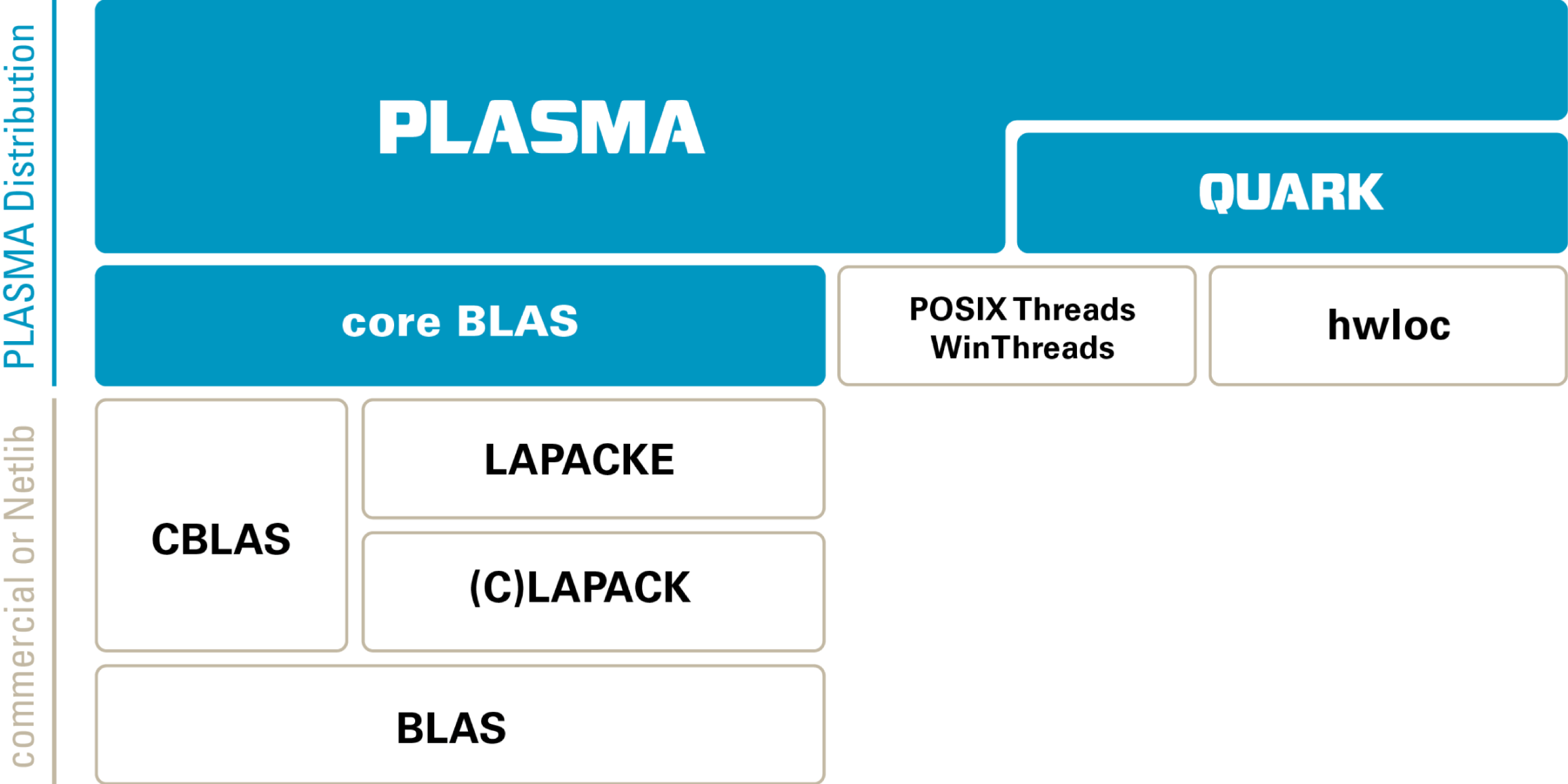
PLASMA is built on top of well-established dense linear algebra software components, and Figure 3.1 shows PLASMA’s software stack. PLASMA relies on the collection of Basic Linear Algebra Subroutines (BLAS: Dongarra et al. Reference Dongarra, Du Croz, Hammarling and Duff1990), available in many commercial packages (e.g. Intel MKL, AMD ACML, IBM ESSL, Cray LibSci), to extract maximum performance from each individual core. Academic implementations of BLAS are also available (e.g. ATLAS, OpenBLAS). PLASMA utilizes the C interface to BLAS (CBLAS), which is part of most BLAS distributions, but is also available from Netlib in the form of C wrappers to the legacy Fortran interface.Footnote 1 PLASMA relies on LAPACK for serial implementations of more complex routines, such as matrix factorizations. Here, PLASMA also utilizes the C interface (LAPACKE), which is distributed by Intel in the MKL software suite, and is also available from Netlib.Footnote 2 PLASMA encapsulates all calls to CBLAS and LAPACKE in the core_blas component, which constitutes the set of all serial building blocks for the parallel algorithms in PLASMA.
The software stack of PLASMA, version 2.7.

The main algorithmic work in PLASMA revolves around efficient multithreading using core_blas components. Initially, PLASMA was developed using static thread scheduling, but high interest in dynamic task scheduling led to the development of the QUARK scheduler (YarKhan, Kurzak and Dongarra Reference YarKhan, Kurzak and Dongarra2011) and gradual introduction of dynamic scheduler routines in PLASMA. PLASMA’s statically scheduled routines follow the single program multiple data (SPMD) programming paradigm, where each thread relies on its thread ID and the total number of threads in the system to figure out its unique path through the workflow. Synchronization is implemented using shared progress tables and busy waiting. PLASMA’s dynamically scheduled routines follow the superscalar programming paradigm, where the code is written sequentially and parallelized at runtime through the analysis of the dataflow between different tasks. As of version 2.7, PLASMA utilizes both types of scheduling, and many routines are available for the two implementations. With the adoption of superscalar scheduling in the OpenMP standard,Footnote 3 transition from QUARK to OpenMP is a very likely path forward for PLASMA.
OpenMP is an API that supports multi-platform shared memory multiprocessing programming in C, C++, and Fortran, on most processor architectures and operating systems, including Linux, Mac OSX, and Windows. It consists of a set of compiler directives, library routines, and environment variables that influence runtime behaviour. OpenMP is an implementation of multithreading, a method of parallelizing whereby a master thread (a series of instructions executed consecutively) forks a specified number of slave threads, and the system divides a task among them. The threads then run concurrently, with the runtime environment allocating threads to different processors. By default, each thread executes the parallelized section of code independently. Work-sharing constructs can be used to divide a task among the threads so that each thread executes its allocated part of the code. Both task parallelism and data parallelism can be achieved using OpenMP in this way.
The OpenMP Architecture Review Board (ARB) published its first API specifications, OpenMP for Fortran 1.0, in October 1997. In October 1998, the C/C++ standard was released. The year 2000 saw version 2.0 of the Fortran specifications, with version 2.0 of the C/C++ specifications being released in 2002. Version 2.5 is a combined C/C++/Fortran specification that was released in 2005. Up until that point, OpenMP provided mostly fork–join parallelism exemplified by the #parallel for construct. Version 3.0, released in May 2008, included the concept of tasks and the task construct, which drew heavily from the Cilk project (Blumofe et al. Reference Blumofe, Joerg, Kuszmaul, Leiserson, Randall and Zhou1995) and was quite limited. Version 4.0 of the specification, released in July 2013, adds or improves the following features: support for accelerators, atomics, error handling, thread affinity, tasking extensions, user-defined reduction, SIMD support, and Fortran 2003 support. Most importantly, from the standpoint of PLASMA, the 4.0 standard fully embraces the concept of scheduling work expressed in the form of a Direct Acyclic Graph (DAG) of tasks, also referred to as superscalar scheduling.
Superscalar scheduling relies on the resolution of data hazards/dependencies: read after write (RaW), write after read (WaR), and write after write (WaW). The read after write (RaW) hazard, often referred to as true dependency, is the most common. It defines the relation between a task of writing (creating) the data and the task of reading (consuming) the data. In that case the latter task has to wait until the former task completes. The write after read (WaR) hazard is caused by a situation where a task attempts to write/modify data before a preceding task has finished reading the data. In such a case, the writer has to wait until the reader completes. The dependency is not referred to as a true dependency, because it can be eliminated by renaming (making a copy) of the data. Although the dependency is unlikely to appear often in dense linear algebra, it has been encountered, and it has to be handled by the scheduler to ensure correctness. The write after write (WaW) hazard is caused by a situation where a task attempts to write data before a preceding task has finished writing the data. The final result is expected to be the output of the latter task, but if the dependency is not preserved (and the former task completes after the latter one), incorrect output will result. This is an important dependency in the hardware design of processor pipelines, where resource contention can be caused by a limited number of registers. The situation is, however, quite unlikely for a software scheduler, where the occurrence of the WaW hazard means that some data are produced and overwritten before being consumed. Like the WaR hazard, the WaW hazard can be removed by renaming.
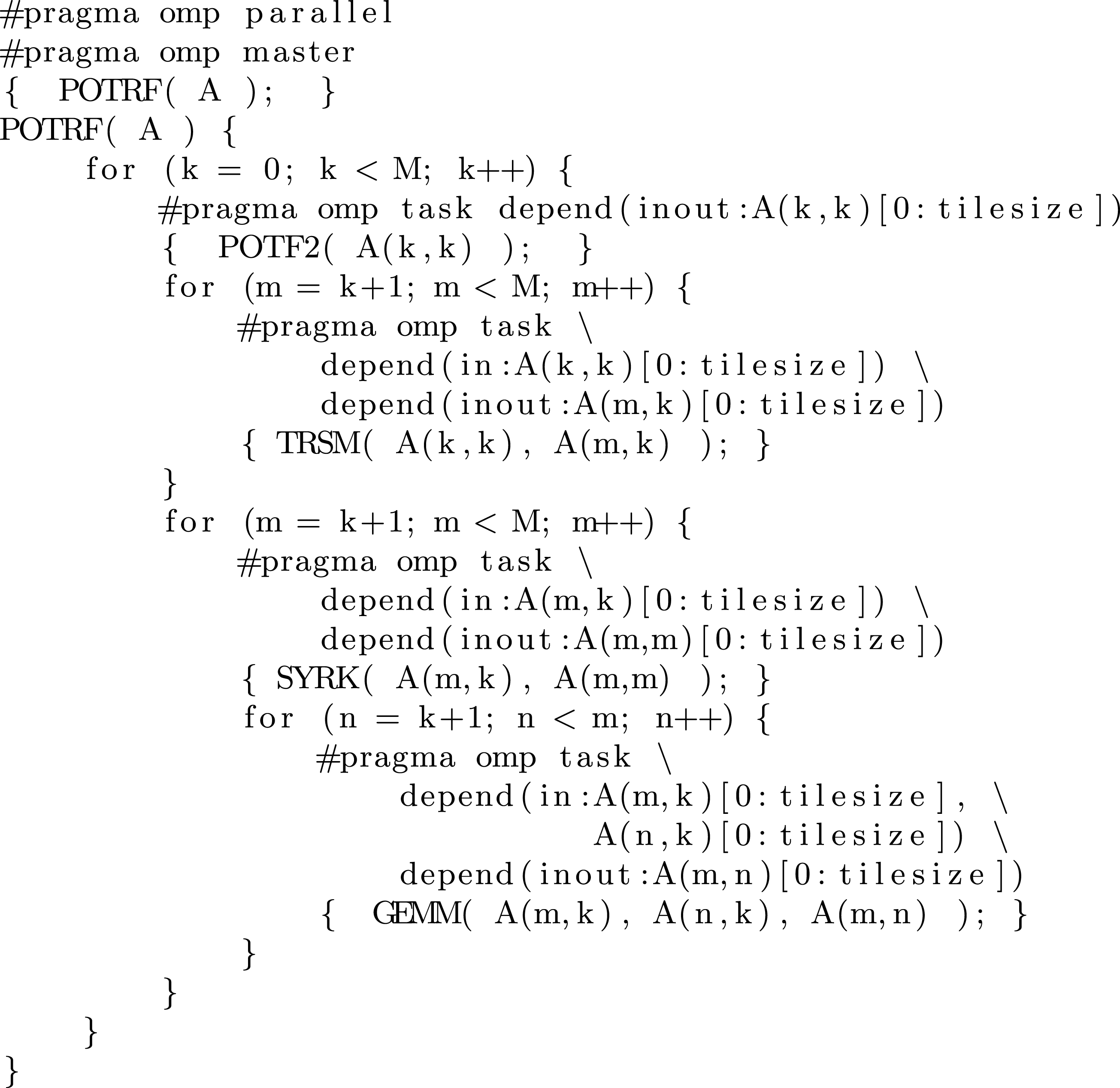
Tile Cholesky algorithm using OpenMP 4.0 tasks with dependencies.

In linear algebra, the Cholesky decomposition or Cholesky factorization is a decomposition of a Hermitian positive definite matrix into the product of a lower triangular matrix and its conjugate transpose. When it is applicable, the Cholesky decomposition is roughly twice as efficient as the LU decomposition for solving systems of linear equations. Figure 3.2 shows the Cholesky factorization expressed using OpenMP 4.0 tasks. The outermost loop iterates over the steps of the factorization. The inner loops iterate over the vertical (m) and horizontal (n) dimensions of the matrix. At each step, a diagonal block A(k,k) is factored (POTRF). Then a triangular solve is used to update all the panel tiles A(m,n) below the diagonal block (TRSM). Finally, all the tiles to the right of the panel (the trailing submatrix) are updated, using a symmetric rank- $k$ update (SYRK) for diagonal tiles A(m,m) and matrix multiplication (GEMM) on the other tiles A(m,n). The #pragma omp task clauses are used to queue tasks for execution and the depend statements are used to specify data dependencies by providing the direction (in/out), the pointer to the data, and the data size.
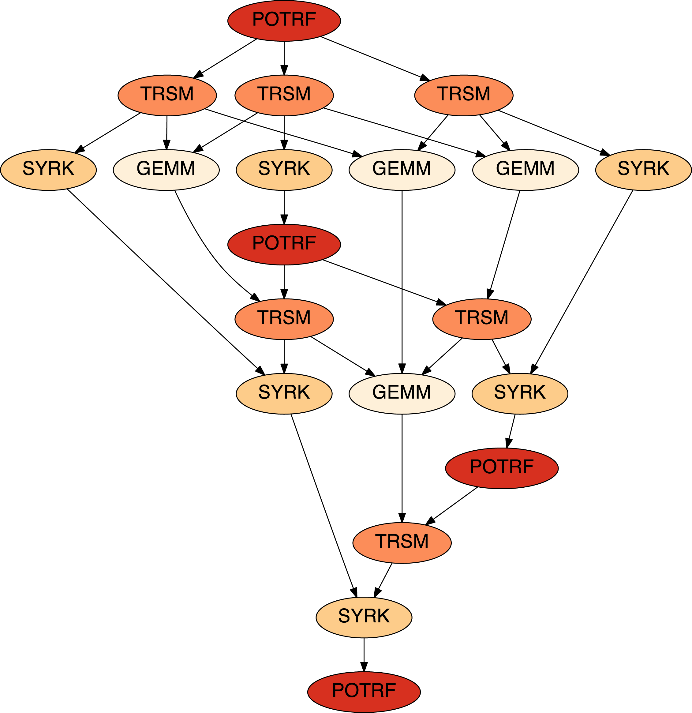
The DAG of a  $4\times 4$ (tiles) Cholesky factorization.
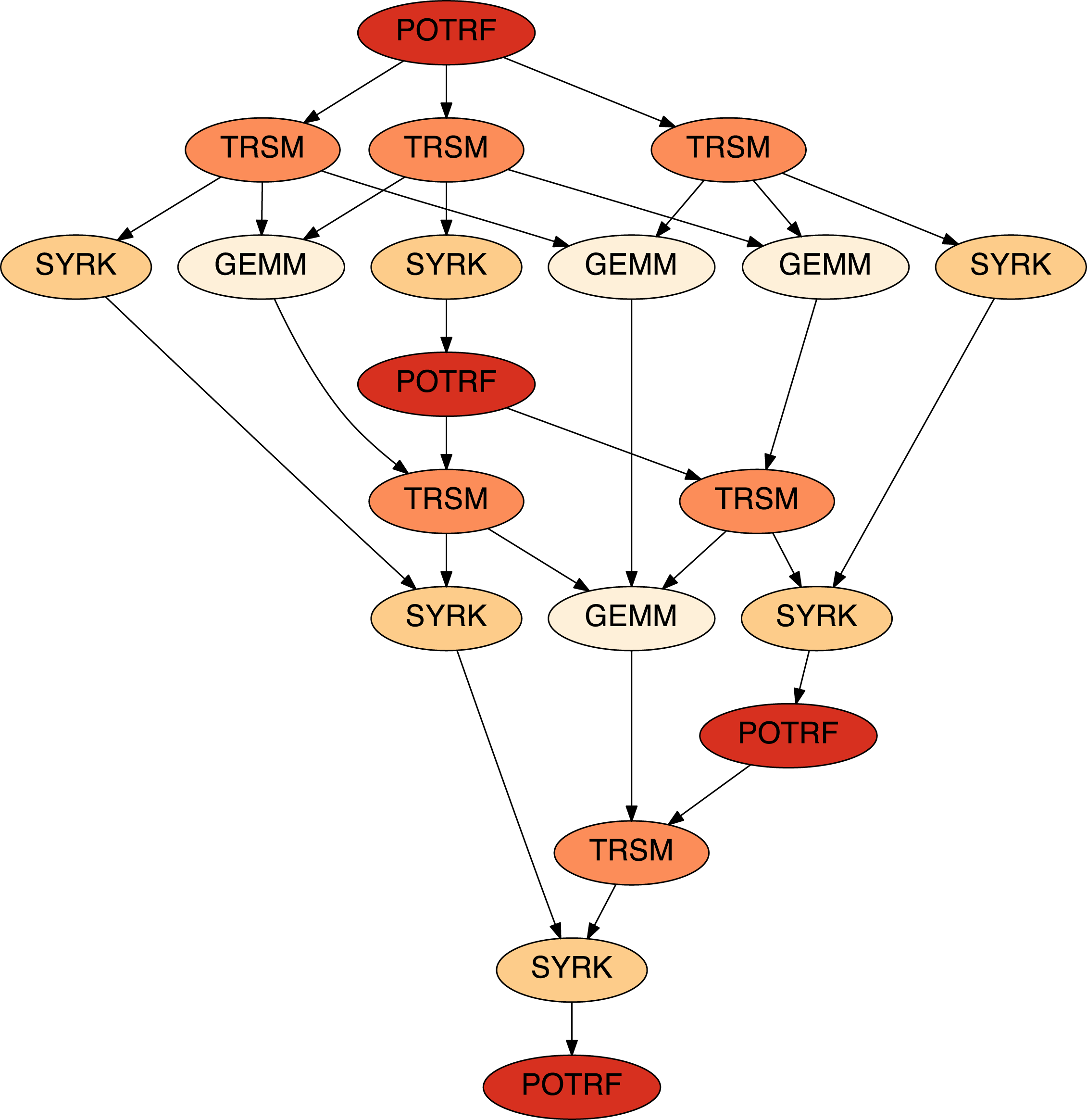
Figure 3.3 shows the DAG of a  $4\times 4$ (tiles) Cholesky factorization. Factorization of the first diagonal block (POTRF) unlocks three triangular solves (TRSM) below that block, which in turn unlock three symmetric rank-
 $k$ updates (SYRK) and three matrix multiplications (GEMM) to the tiles of the trailing submatrix. One of the SYRK operations updates the second diagonal block, which unlocks the factorization of that block (the second POTRF). This process continues until the last diagonal block is factored (the POTRF at the bottom of the DAG), which concludes the factorization of the matrix.
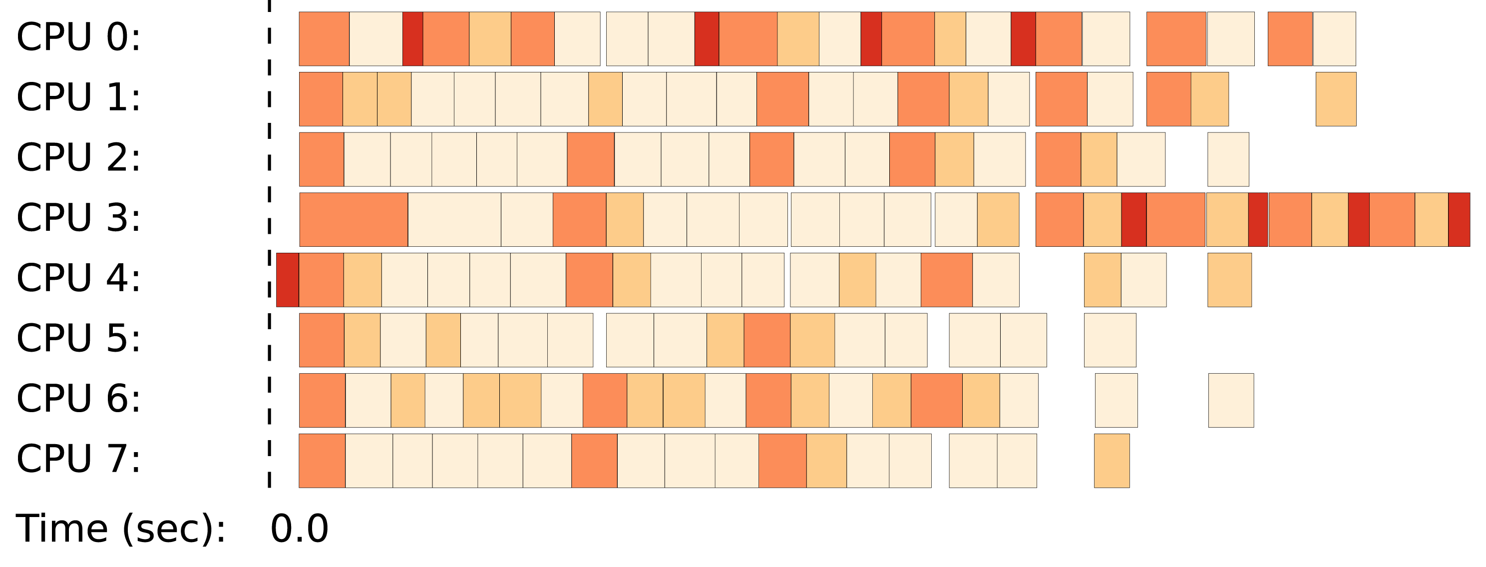
Trace of a  $9\times 9$ (tiles) Cholesky factorization.

Figure 3.4 shows an execution trace of a larger,  $9\times 9$ (tiles), Cholesky factorization using eight cores. Here, the first POTRF task unlocks eight TRSM tasks, which in turn unlock many more SYRK and GEMM tasks. Due to dynamic scheduling, there are no clear boundaries between the steps of the factorization. Instead, operations are well pipelined until the cores run out or work at the end of the factorization. The last operations (TRSM, SYRK, POTRF) are serialized due to a chain of dependencies in the DAG.
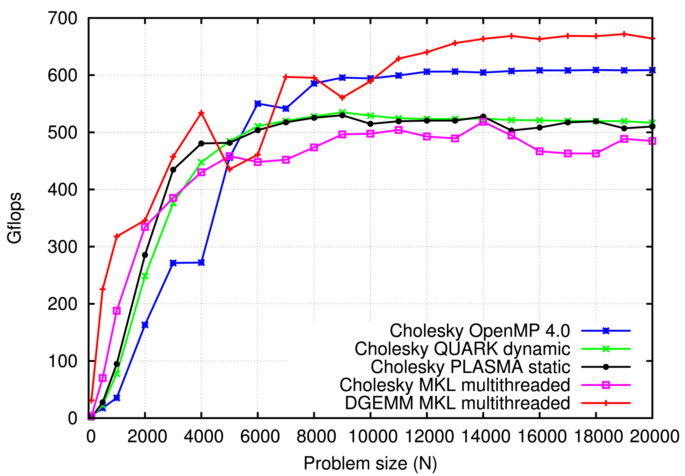
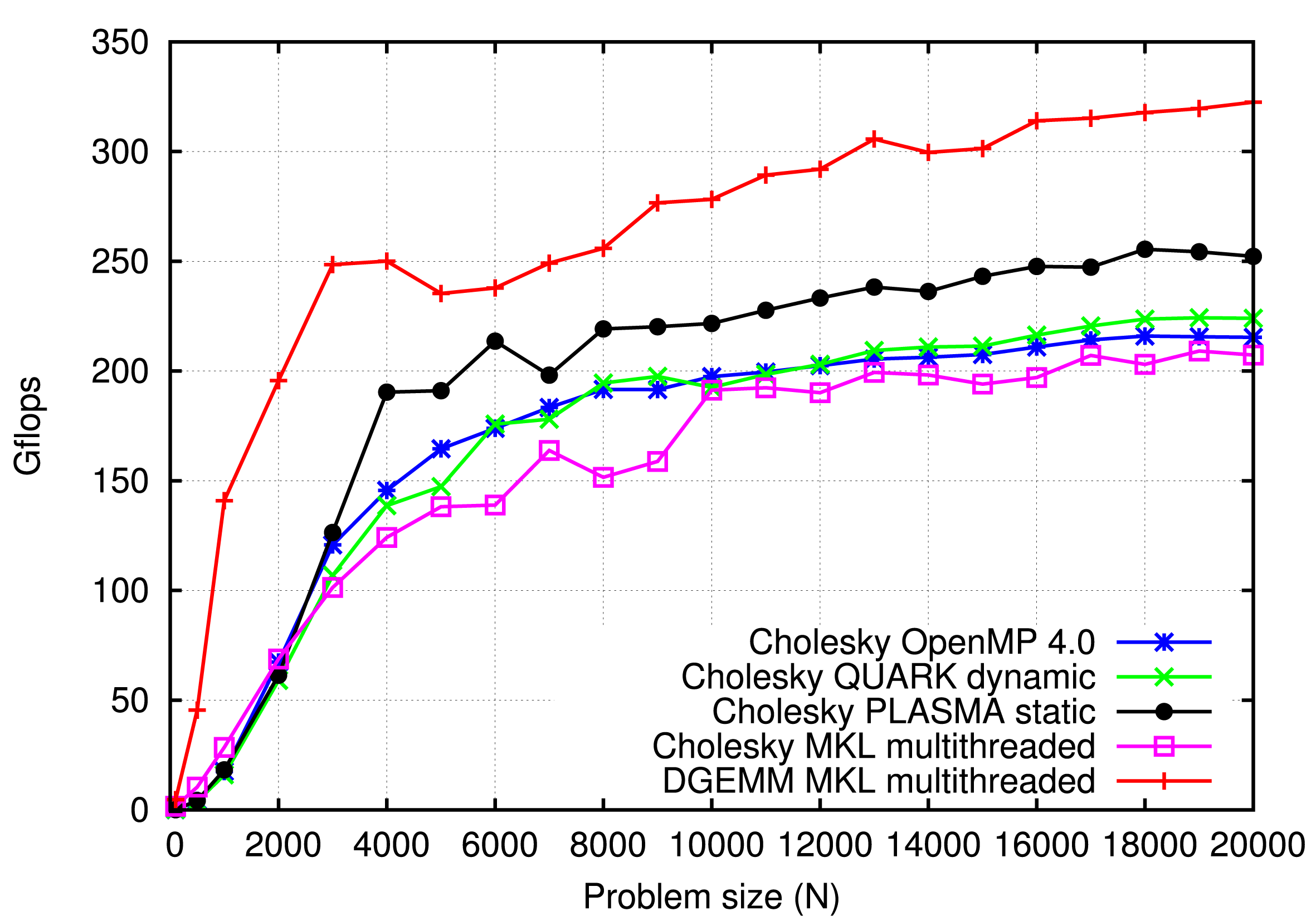
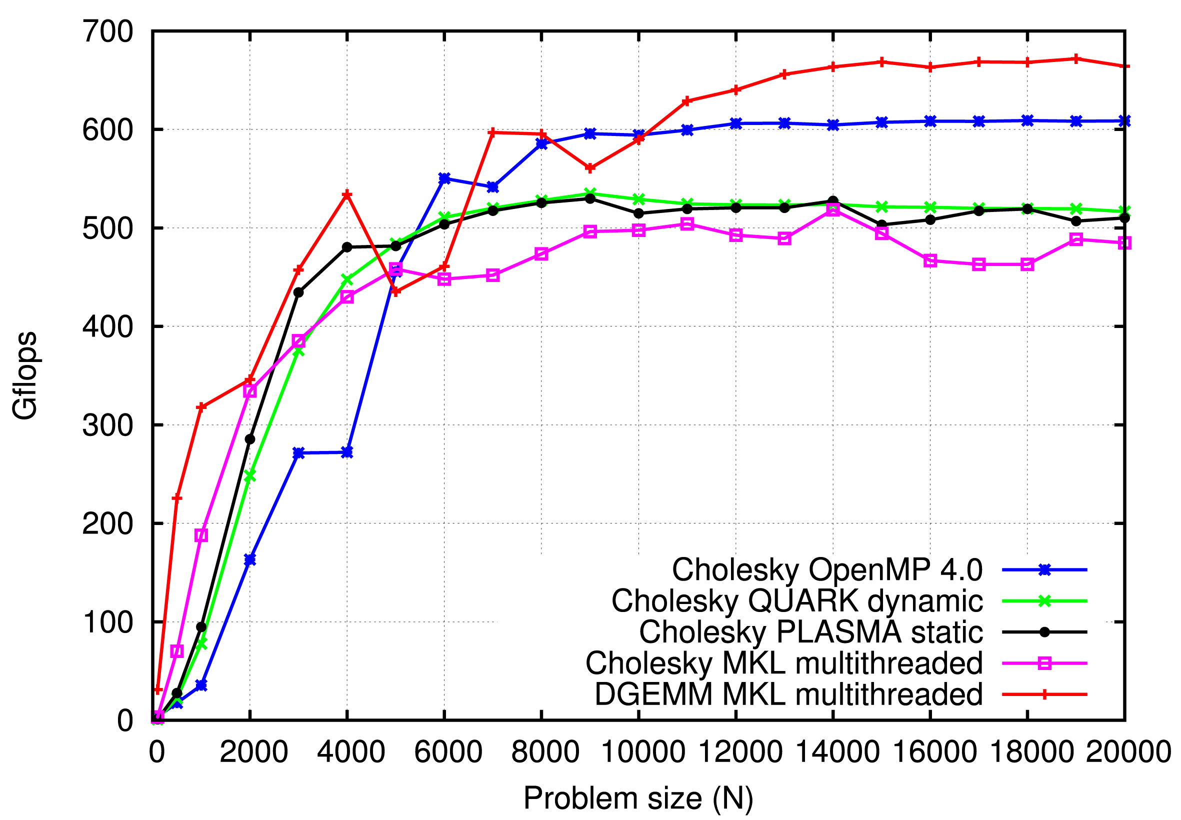
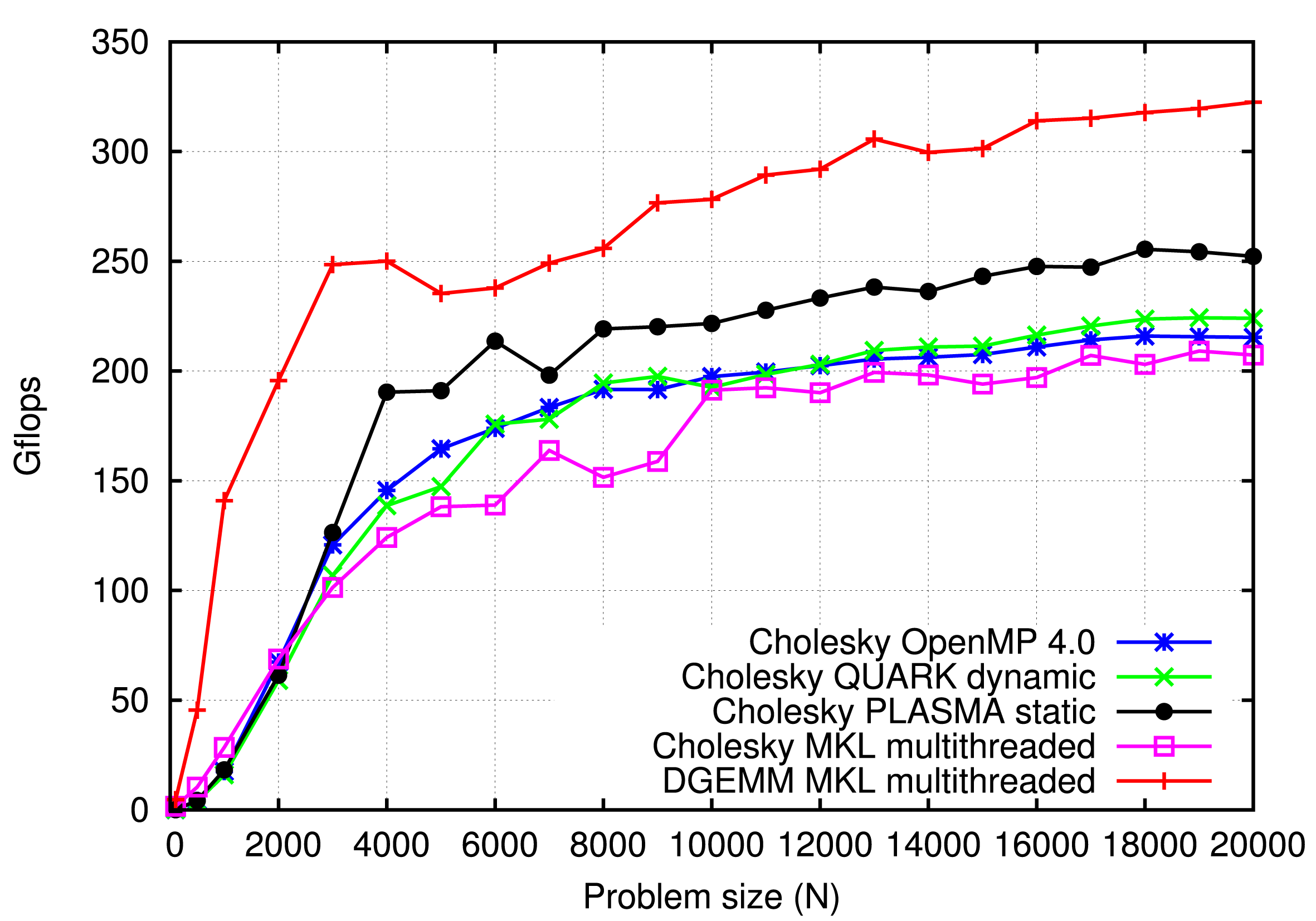
Figure 3.5 compares the performance of different implementations using a dual-socket, 20-core, Intel Haswell system, while Figure 3.6 compares the performance using an eight-socket, 48-core AMD Istanbul system. All codes were compiled using the GCC compiler and linked against the MKL library. In both cases the DGEMM routine from MKL is used as a reference point (basically the upper bound of performance). In the case of the Haswell system, OpenMP delivers performance which matches or exceeds the performance of all the other systems, including: QUARK, PLASMA static scheduling, and the DPOTRF routine from MKL. In the case of the Istanbul system, OpenMP delivers performance better than MKL, almost identical to QUARK and slightly lower than PLASMA static scheduling. In this case, the gap to the static scheduling can probably be closed by further tuning.
Cholesky factorization performance: DPOTRF Intel Xeon E5-2650 v3 (Haswell) 2.3 GHz, 20 cores.
Cholesky factorization performance: DPOTRF AMD Opteron 8439 SE (Istanbul) 2.8 GHz, 48 cores (8 sockets, 6 cores).
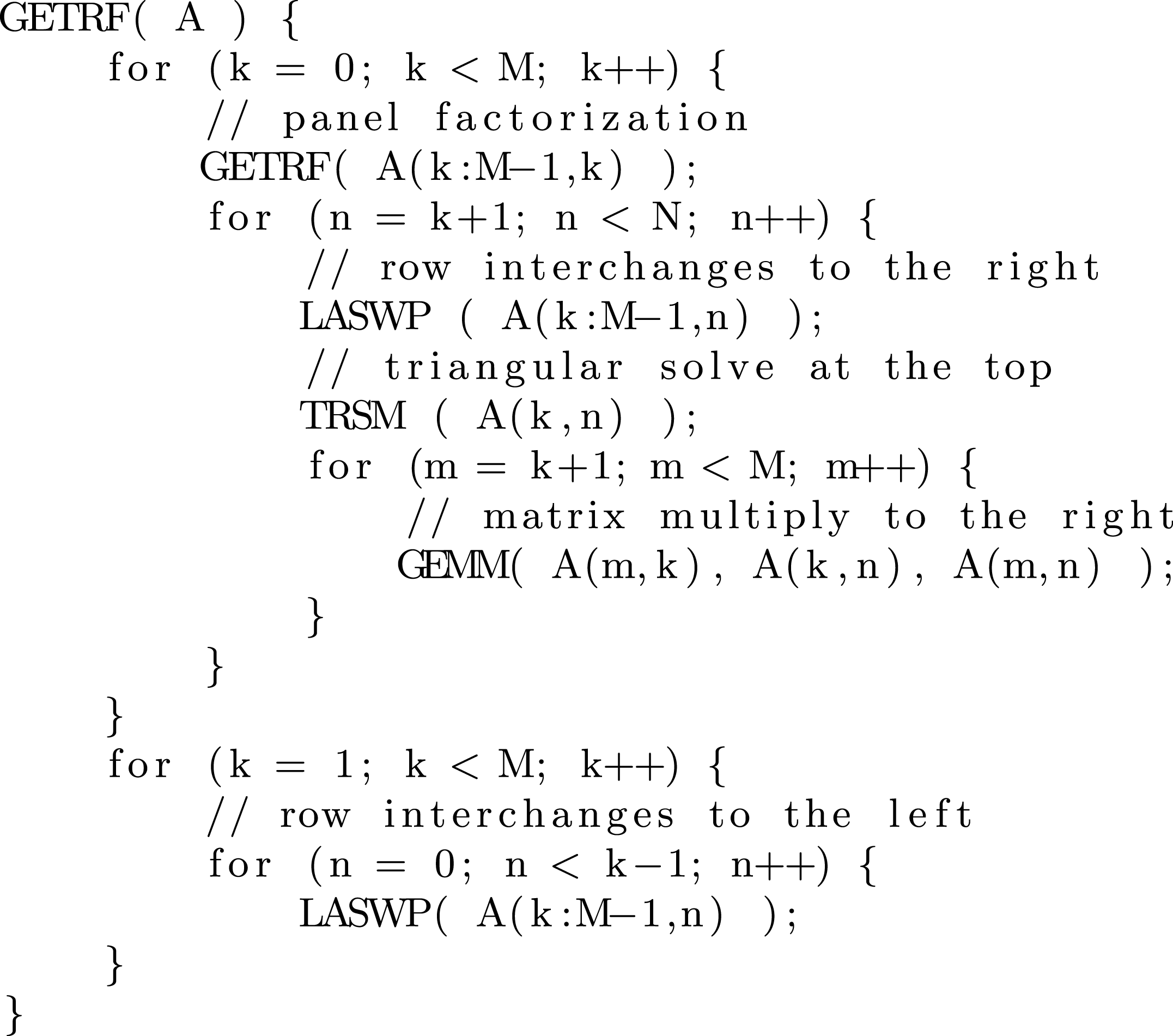
A slightly more challenging problem is that of scheduling the LU decomposition. LU decomposition (where ‘LU’ stands for ‘lower upper’, and is also called LU factorization) factors a matrix as the product of a lower triangular matrix and an upper triangular matrix. The product sometimes includes a permutation matrix as well. The LU decomposition can be viewed as the matrix form of Gaussian elimination. Computers usually solve square systems of linear equations using the LU decomposition, and it is also a key step when inverting a matrix, or computing the determinant of a matrix. The OpenMP 4.0 implementation of the LU factorization is considerably more complex than the Cholesky factorization. Therefore, Figure 3.7 shows a serial implementation of the LU factorization instead of the actual OpenMP 4.0 implementation. At each step, a block of columns (a panel) is factored (GETRF). Within the panel factorization, partial (row) pivoting is applied and a pivoting pattern is created. That pivoting pattern is then applied to the trailing submatrix through a series of row interchanges (LASWP). Then a block of top rows is updated with a triangular solve (TRSM), and finally, all the tiles to the right of the panel are updated, using matrix multiplication (GEMM). At the end of the factorization, row interchanges are applied to the left of each panel.
Serial LU factorization.

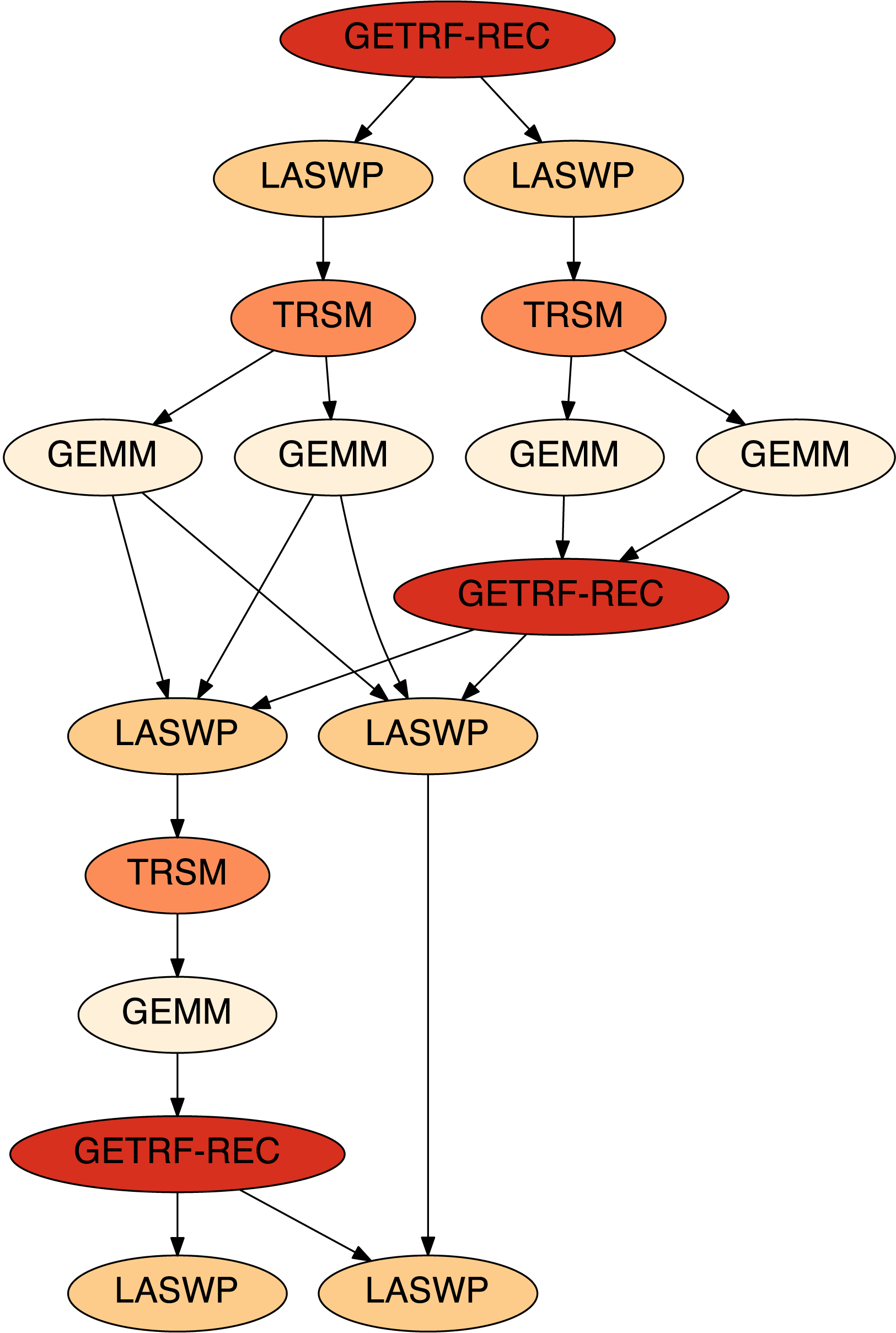
The DAG of a  $3\times 3$ (tiles) LU factorization.
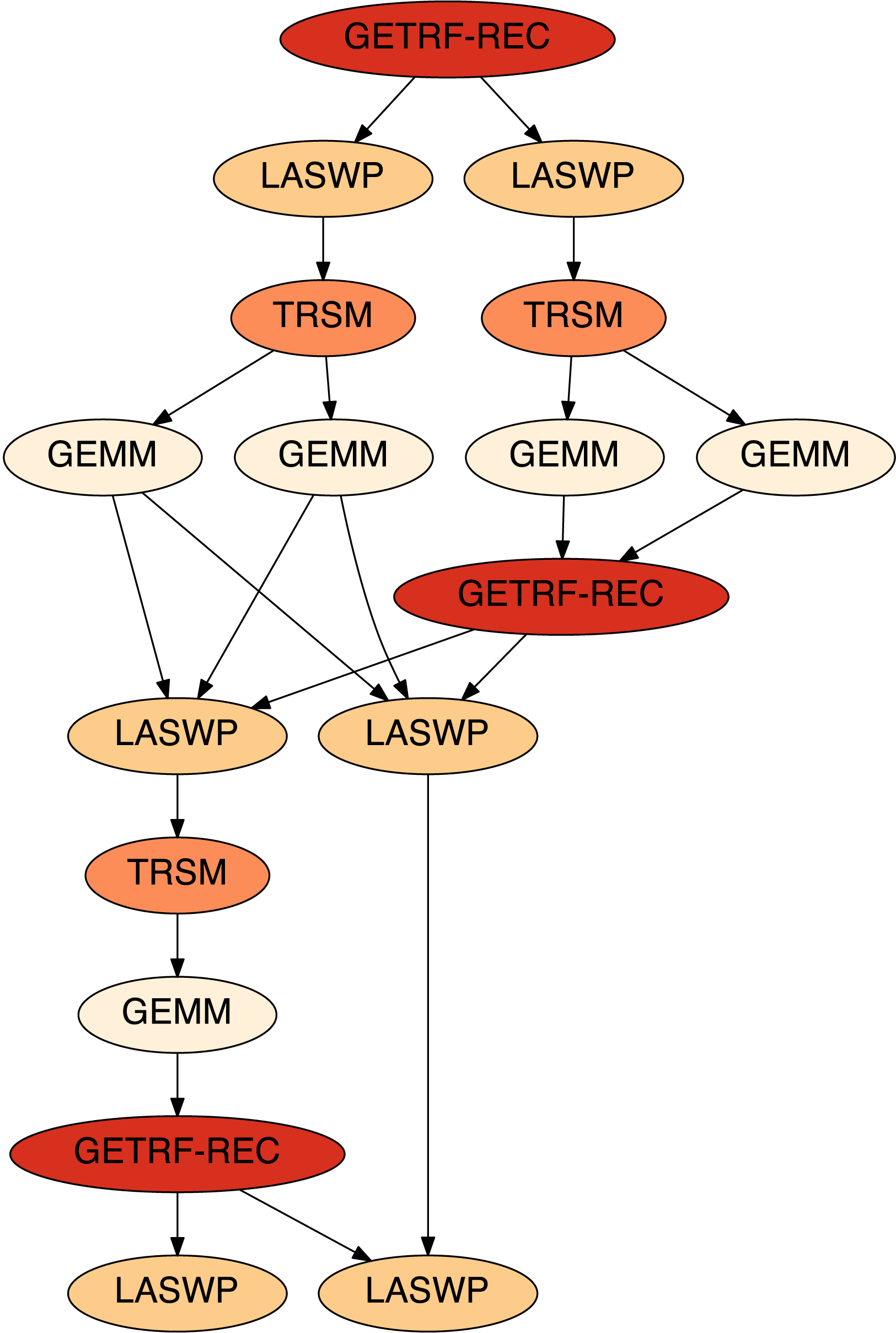
Figure 3.8 shows the DAG of a  $3\times 3$ (tiles) LU factorization. The first task is the factorization of the first block of columns (panel). Since this is a demanding task, located in the critical path of the algorithm, PLASMA utilizes a very fast, cache-friendly, recursive, multithreaded implementation of this operation, as indicated by the ‘REC’ postfix in the ‘GETRF-REC’ label. This task unlocks row interchanges to the right of the panel (LASWP) due to the partial row pivoting technique. They, in turn, unlock triangular solves in the top block of rows (TRSMs), followed by matrix multiplications to update the remainder of the matrix (GEMMs). Two of those GEMM operations update the second panel, and therefore unlock the second GETRF-REC task, and so on. The increased complexity of multithreading the LU factorization stems from the fact that the panel factorization task (GETRF-REC) spans an entire column of tiles, and is internally multithreaded using low-level constructs for synchronization (locks, atomics).
Figure 3.9 shows an execution trace of a larger,  $10\times 10$ (tiles), LU factorization using eight cores. The first task is the multithreaded GETRF-REC task. In this small example it only uses two threads, and only in the first three steps of the factorization. More threads would be used in a larger case. Completion of the GETRF-REC task unlocks nine LASWP tasks, which in turn unlock nine TRSM tasks, which in turn unlock many more GEMM tasks. Notably, factorization of the second panel can proceed concurrently with the GEMM updates from the first step, factorization of the third panel can proceed concurrently with the GEMM updates from the second step, and so on. Operations are well pipelined until work runs out towards the end of the factorization.
Trace of a  $10\times 10$ (tiles) LU factorization.

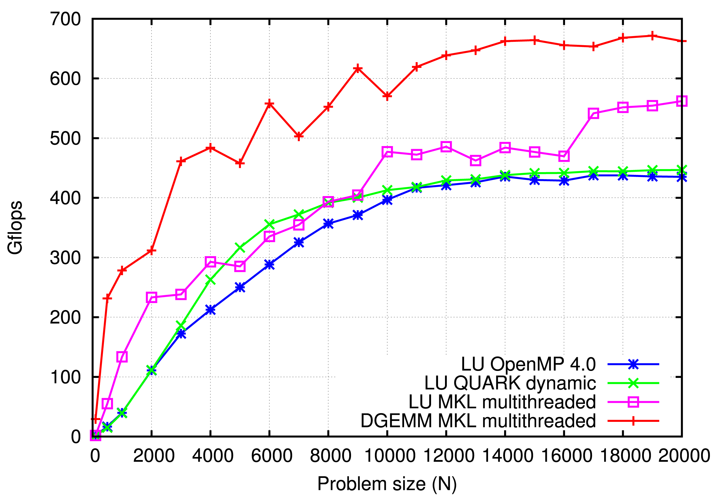
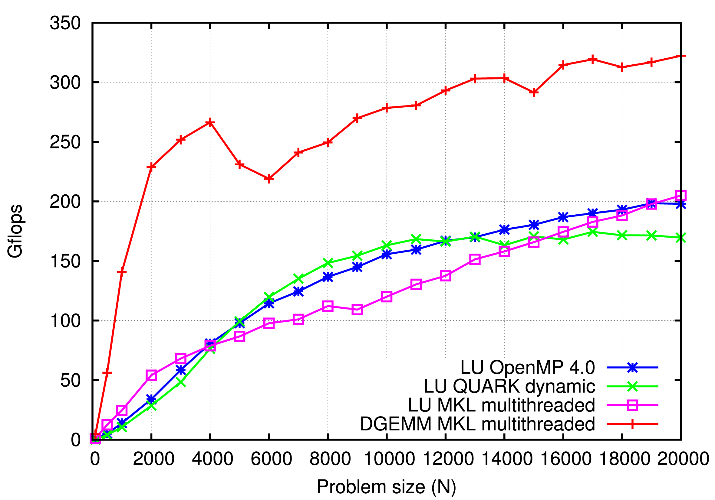
Figure 3.10 compares the performance of different implementations using a dual-socket, 20-core, Intel Haswell system, while Figure 3.11 compares the performance using an eight-socket, 48-core AMD Istanbul system. All codes were compiled using the GCC compiler and linked against the MKL library. In both cases the DGEMM routine from MKL is used as a reference point (the performance upper bound). In the case of the Haswell system, OpenMP delivers slightly lower performance than QUARK and MKL. In the case of the Istanbul system, OpenMP delivers performance almost identical to MKL, and slightly lower than QUARK up to 16 000 and slightly higher beyond that point. OpenMP’s performance can, most likely, be improved by further tuning.
LU factorization performance: DGETRF Intel Xeon E5-2650 v3 (Haswell) 2.3 GHz, 20 cores.

LU factorization performance: DGETRF AMD Opteron 8439 SE (Istanbul) 2.8 GHz, 48 cores (8 sockets, 6 cores).

In summary, the superscalar scheduling capabilities of OpenMP 4.0 provide many benefits over a proprietary scheduling system. By being language extensions, OpenMP directives produce much more compact and readable codes. By being a standard, OpenMP provides portability to different operating systems, and solves a multitude of lower-level problems, such as thread affinity, etc. At the same time, the GCC implementation provides performance that matches or exceeds that of other similar systems. Therefore, OpenMP seems to be a clear path forward for multithreaded numerical libraries that require sophisticated scheduling, such as PLASMA.
3.2 Distributed memory scheduling in DPLASMA
Distributed parallel linear algebra software for multicore architectures (or DPLASMA) is a distributed memory counterpart of PLASMA. DPLASMA contains a subset of PLASMA routines, including routines for solving linear systems of equations and least-squares problems, reductions to condensed form (block-bidiagonal, block-tridiagonal), and a full set of Level 3 BLAS. DPLASMA supports real and complex arithmetic and in single and double precision. DPLASMA targets systems with large numbers of interconnected nodes, where each node may contain multiple sockets of multicore processors and multiple GPU accelerators or Xeon Phi coprocessors. DPLASMA has been designed to supersede ScaLAPACK (Blackford et al. Reference Blackford, Choi, Cleary, D’Azevedo, Demmel, Dhillon, Dongarra, Hammarling, Henry, Petitet, Stanley, Walker and Whaley1997), mainly by restructuring the software to use dataflow runtime scheduling.
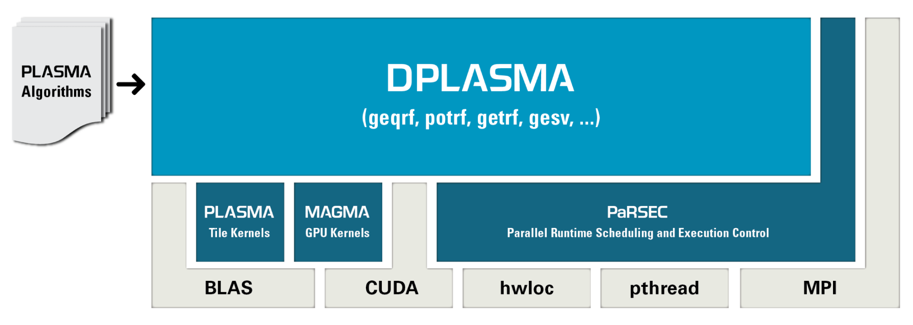
DPLASMA is built on top of a few more components than PLASMA. Figure 3.12 shows DPLASMA’s software stack. In addition to requiring PLASMA and its subcomponents (BLAS, etc.), DPLASMA also relies on their GPU counterparts (MAGMA, cuBLAS, etc.) The scheduling component of DPLASMA is the parallel runtime scheduler and execution controller (PaRSEC), which manages multithreading using Pthreads, message passing using MPI, and accelerator offload using CUDA.
The software stack of PLASMA, version 1.2.

PaRSEC is a generic framework for architecture-aware scheduling and management of micro-tasks on distributed many-core heterogeneous architectures. Workloads are expressed as DAGs of tasks with labelled edges designating data dependencies. DAGs are represented in a compact problem-size independent format that can be queried on-demand to discover data dependencies in a completely distributed fashion. PaRSEC assigns computation threads to the cores, overlaps communications and computations, and uses a dynamic fully distributed scheduler.
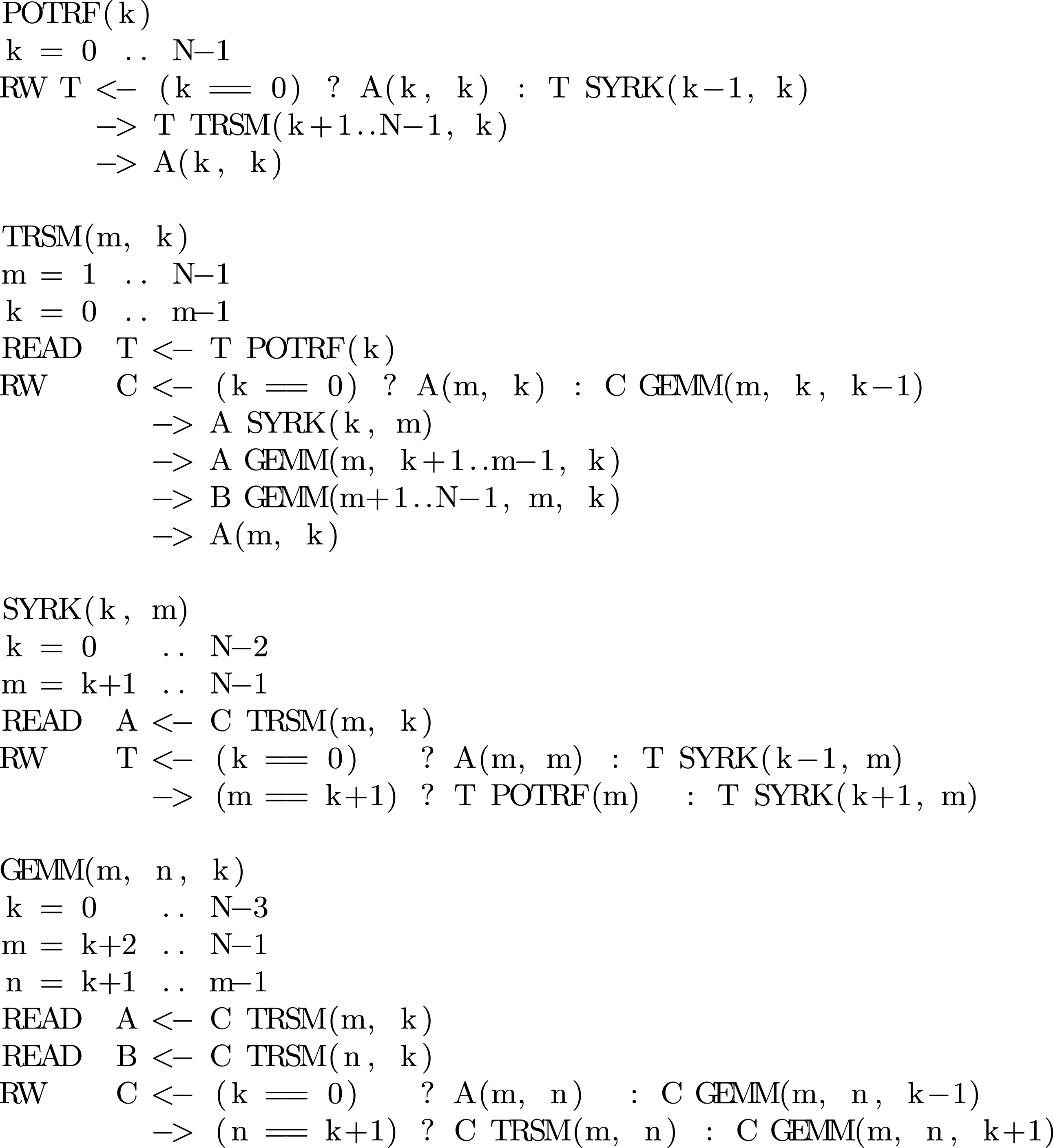
PaRSEC relies on the concept of a parametrized task graph (PTG), which is a size-independent representation of a DAG. The notation used in PaRSEC is called job dependency format (JDF). Figure 3.13 shows the JDF for the Cholesky factorization. The four sections correspond to the four types of tasks used in the factorization: POTRF, TRSM, SYRK, and GEMM. The JDF defines the execution space for each task and the dependencies for all its parameters. Every individual task in the DAG is uniquely identified by a tuple. For instance, the POTRF tasks are identified by the  $k$ index in the range from
 $0$ to
 $N-1$, while the TRSM tasks are identified by the
 $(m,k)$ tuple, where m is in the range from
 $1$ to
 $N-1$ and
 $k$ is in the range from
 $0$ to
 $m-1$. The POTRF has a single read/write parameter
 $T$. In the first step (
 $k==0$) the data come from the memory (
 $A(k,k)$). In the follow-up steps, it comes from the SYRK task of coordinates (
 $k-1,k$). After the task executes, the result is forwarded to a set of TRSM tasks of coordinates (
 $k+1..N-1,k$), and is also returned to the memory (
 $A(k,k)$). In this case forwarding the result from a single source task to multiple destination tasks produces a broadcast pattern.
Tile Cholesky algorithm expressed using the JDF notation.
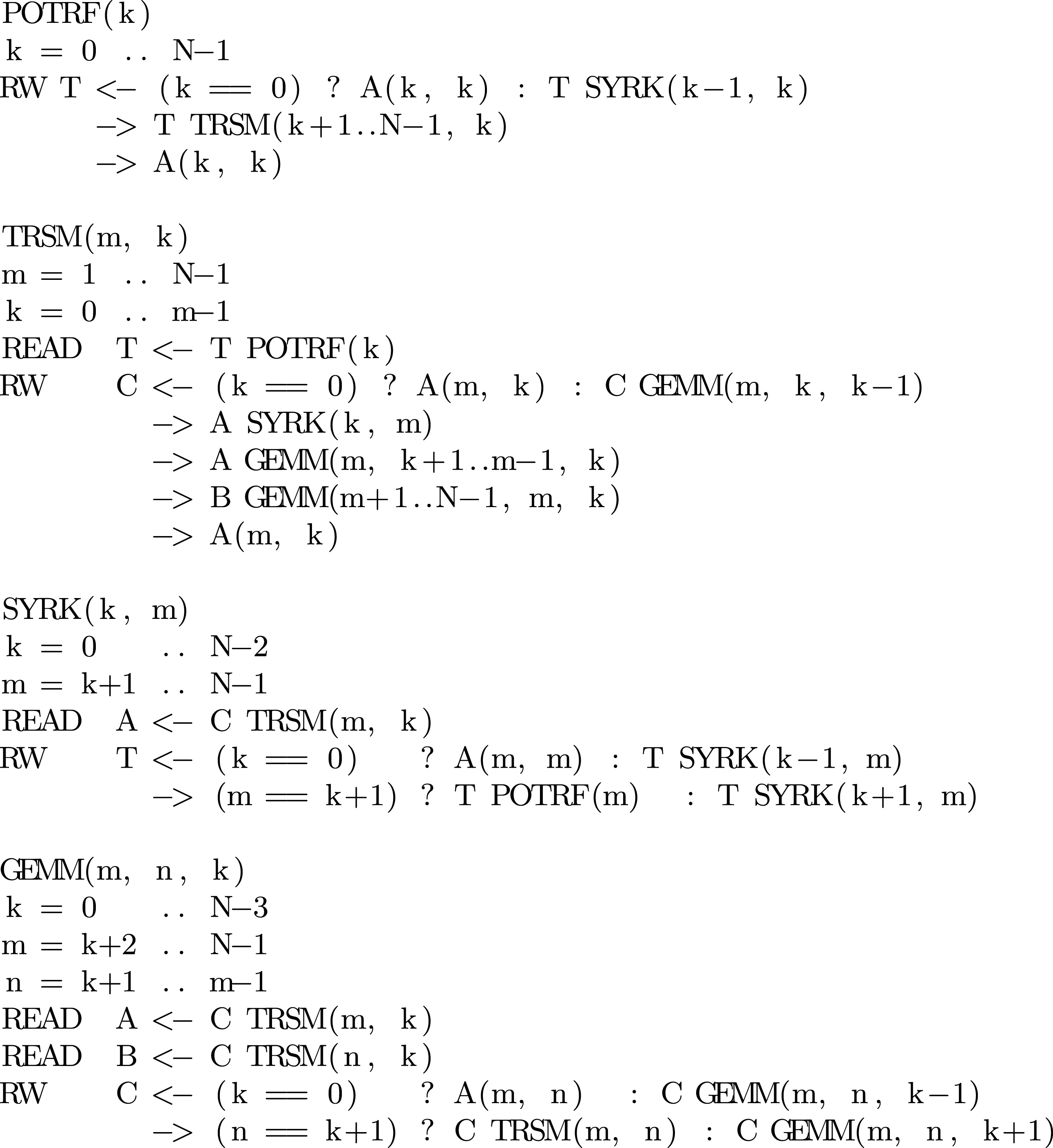
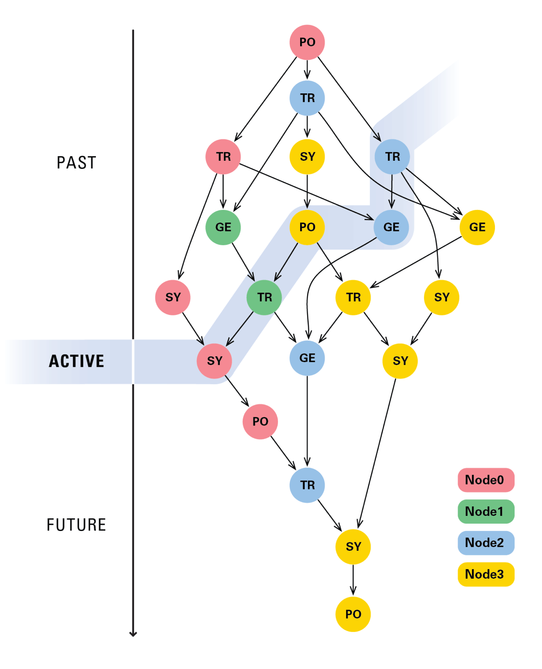
Figure 3.14 shows the principles of PaRSEC execution using the DAG of the Cholesky factorization as an example. While the tasks are statically partitioned to nodes, the execution proceeds dynamically by only activating a small portion of the DAG at a time. Execution is asynchronous and communication is hidden, to the best ability of the hardware (i.e., MPI messages and PCI transfers take place while CPU cores and GPU devices are occupied with useful work, given that the code is rich enough in computation to hide the communication). For efficient management of the memories of multiple GPUs, PaRSEC implements its own GPU memory allocator and applies the replacement policy if memory is exhausted. Currently, PaRSEC applies the least recently used (LRU) policy. More sophisticated approaches are possible.
DAG execution in PaRSEC.
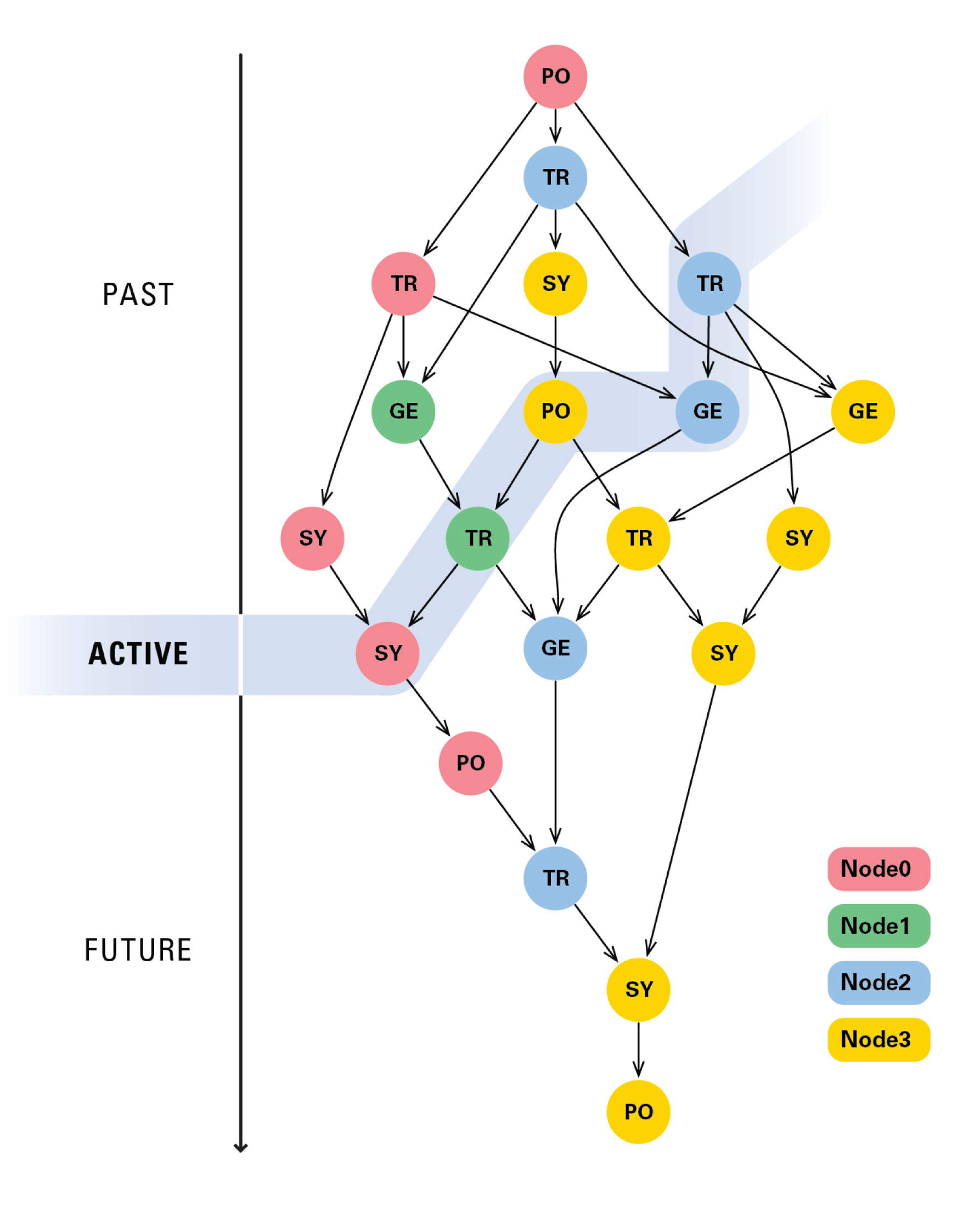
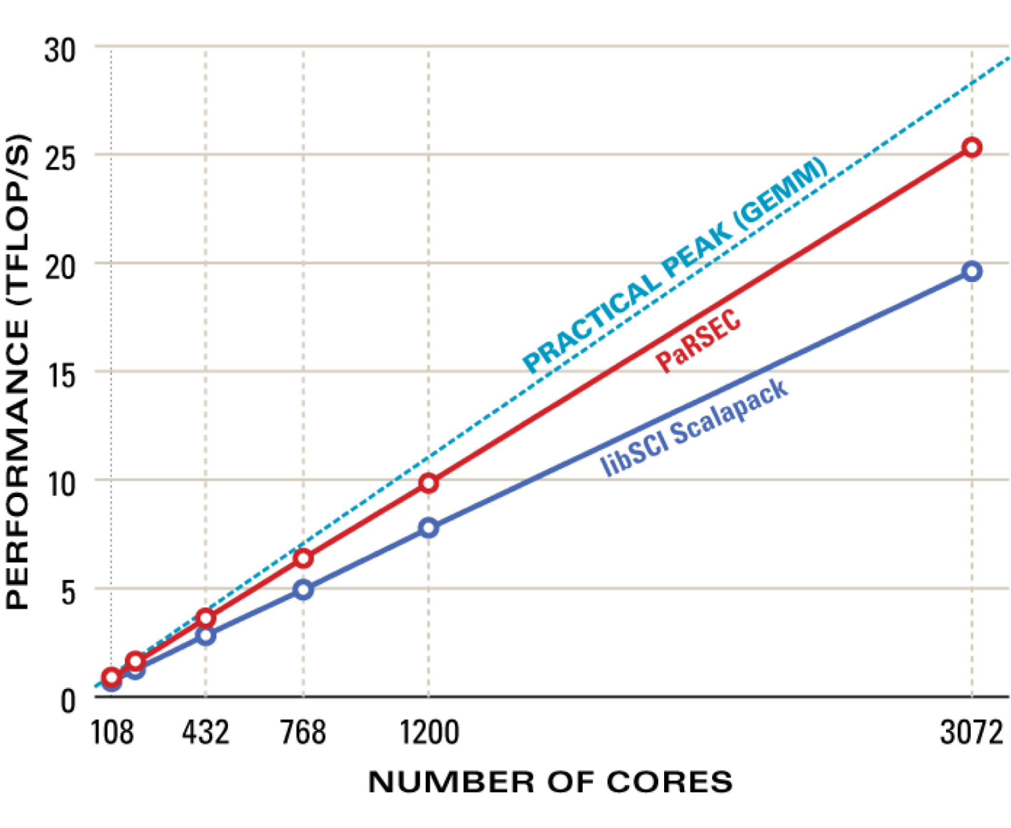
Figure 3.15 compares the performance of PaRSEC to ScaLAPACK, and the theoretical peak when executing the Cholesky factorization in double precision (DPOTRF) on a Cray XT5 system, using up to  $3072$ CPU cores. It is a weak scaling comparison (i.e., the size of the matrix grows as the core count grows, such that the data size per core remains constant). The Cray implementation of ScaLAPACK is used (LibSci). While LibSci’s performance approaches 20 Tflops, PaRSEC’s performance crosses 25 Tflops, an improvement of
 ${\sim}$25%. At the same time, PaRSEC gets within 10% of the theoretical peak.
Cholesky factorization performance: DPOTRF Cray XT5 (Kraken).
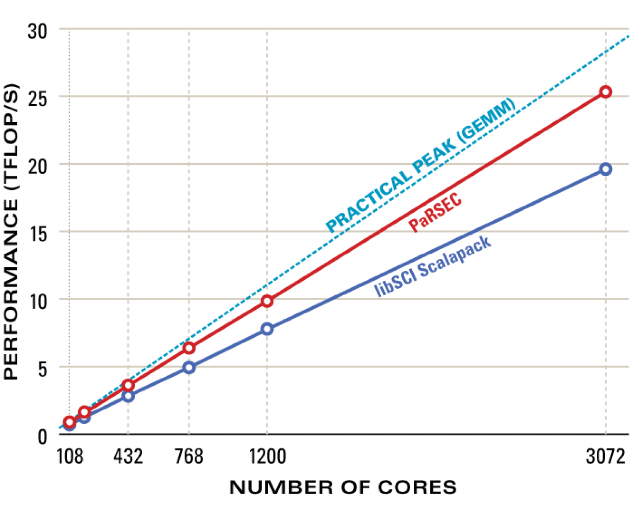
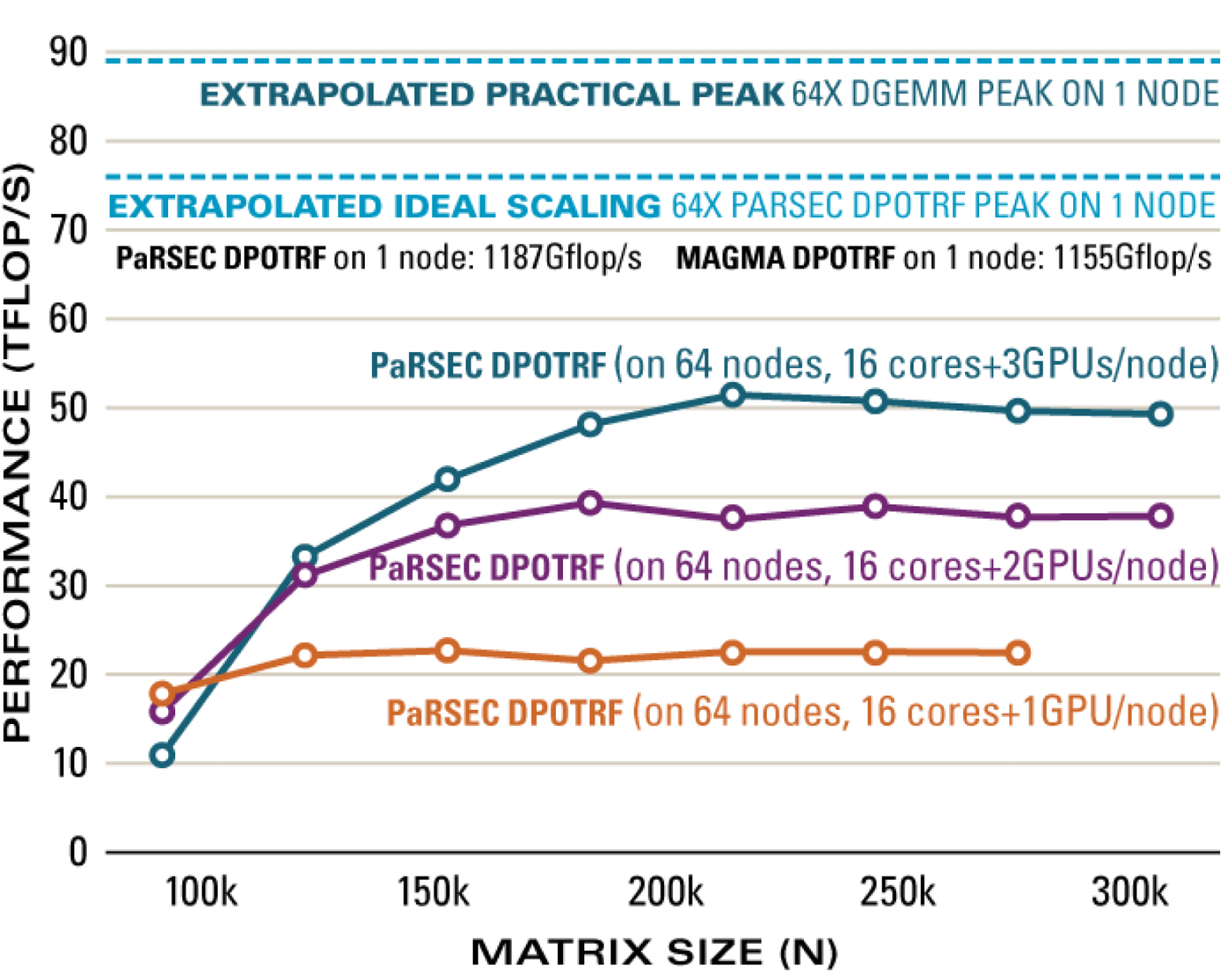
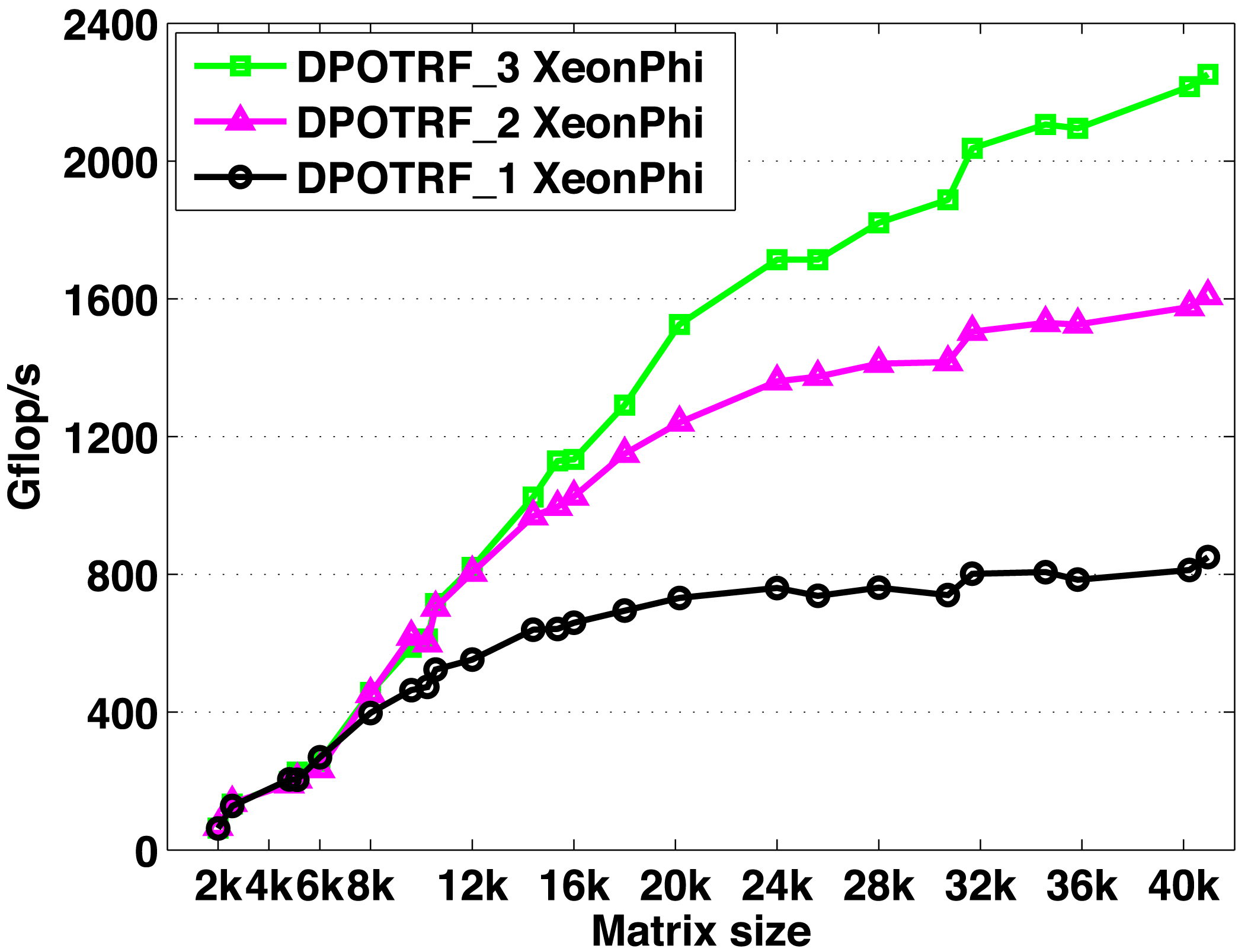
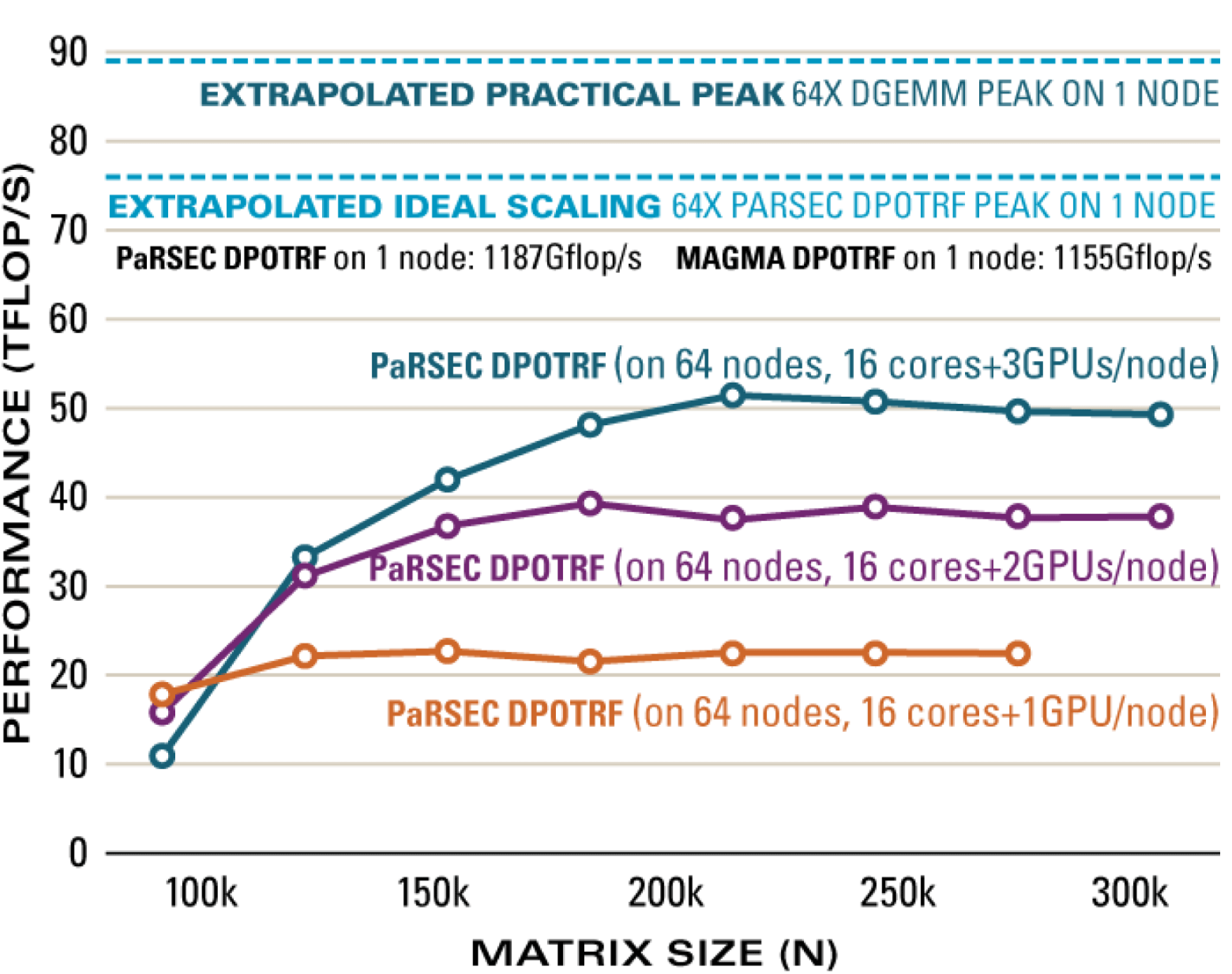
Figure 3.16 shows the performance of PaRSEC executing the DPOTRF routine on a hybrid system, with 64 nodes including three NVIDIA GPUs per node. Performance is shown using a single GPU per node, two GPUs per node, and all three GPUs per node. When using all 192 GPUs, performance of 50 Gflops is achieved for a matrix of size  $200\,000$.
Cholesky factorization performance: distributed hybrid DPOTRF Keeneland 64 nodes (1024 cores, 192 M2090 GPUs, InfiniBand 20G).
4 LU factorization
Gaussian elimination has a long history that can be traced back some  $2000$ years (Grcar Reference Grcar2011). Today, dense systems of linear equations have become a critical cornerstone for some of the most compute-intensive applications. A sampling of domains using dense linear equations include fusion reactor modelling (Jaeger et al. Reference Jaeger, Harvey, Berry, Myra, Dumont, Philips, Smithe, Barrett, Batchelor, Bonoli, Carter, D’Azevedo, D’Ippolito, Moore and Wright2006), aircraft design (Quaranta and Drikakis Reference Quaranta and Drikakis2009), acoustic scattering (Bendali, Boubendir and Fares Reference Bendali, Boubendir and Fares2007), antenna design, and radar cross-section studies (Zhang et al. Reference Zhang, Taylor, Sarkar, Moon and Yuan2008). Simulating fusion reactors, for instance, generates dense systems that exceed half a million unknowns, which are solved using LU factorization (Barrett et al. Reference Barrett, Chan, D’Azevedo, Jaeger, Wong and Wong2010). Many dense linear systems arise from the solution of boundary integral equations via boundary element methods (Edelman Reference Edelman1993), variously called the method of moments in electromagnetics (Harrington Reference Harrington1990), and the panel method in fluid dynamics (Hess Reference Hess1990). These methods replace a sparse three-dimensional problem of
 $O(n^{3})$ unknowns with a dense two-dimensional problem of
 $O(n^{2})$ unknowns. Any improvement in the time to solution for dense linear systems has a direct impact on the execution time of these applications.
4.1 Algorithms
4.1.1 Partial pivoting
The LAPACK block LU factorization is the main point of reference here, and the LAPACK naming convention is followed. The initial ‘D’ in names denotes double precision routines. The LU factorization of a matrix  $A$ has the form
 $$\begin{eqnarray}PA=LU,\end{eqnarray}$$
where  $L$ is a unit lower triangular matrix,
 $U$ is an upper triangular matrix, and
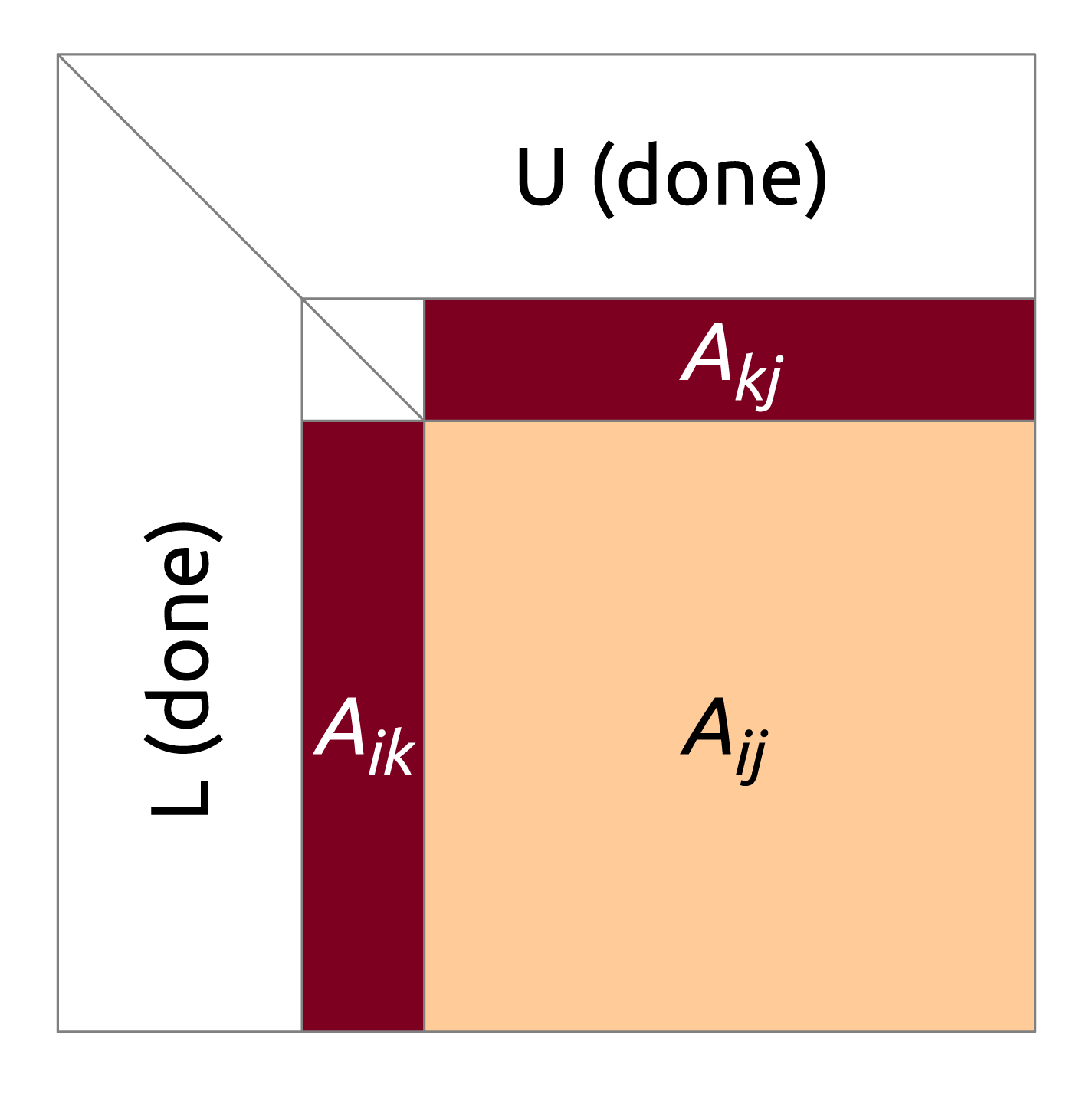
 $P$ is a permutation matrix. The LAPACK algorithm proceeds in the following steps. Initially, a set of
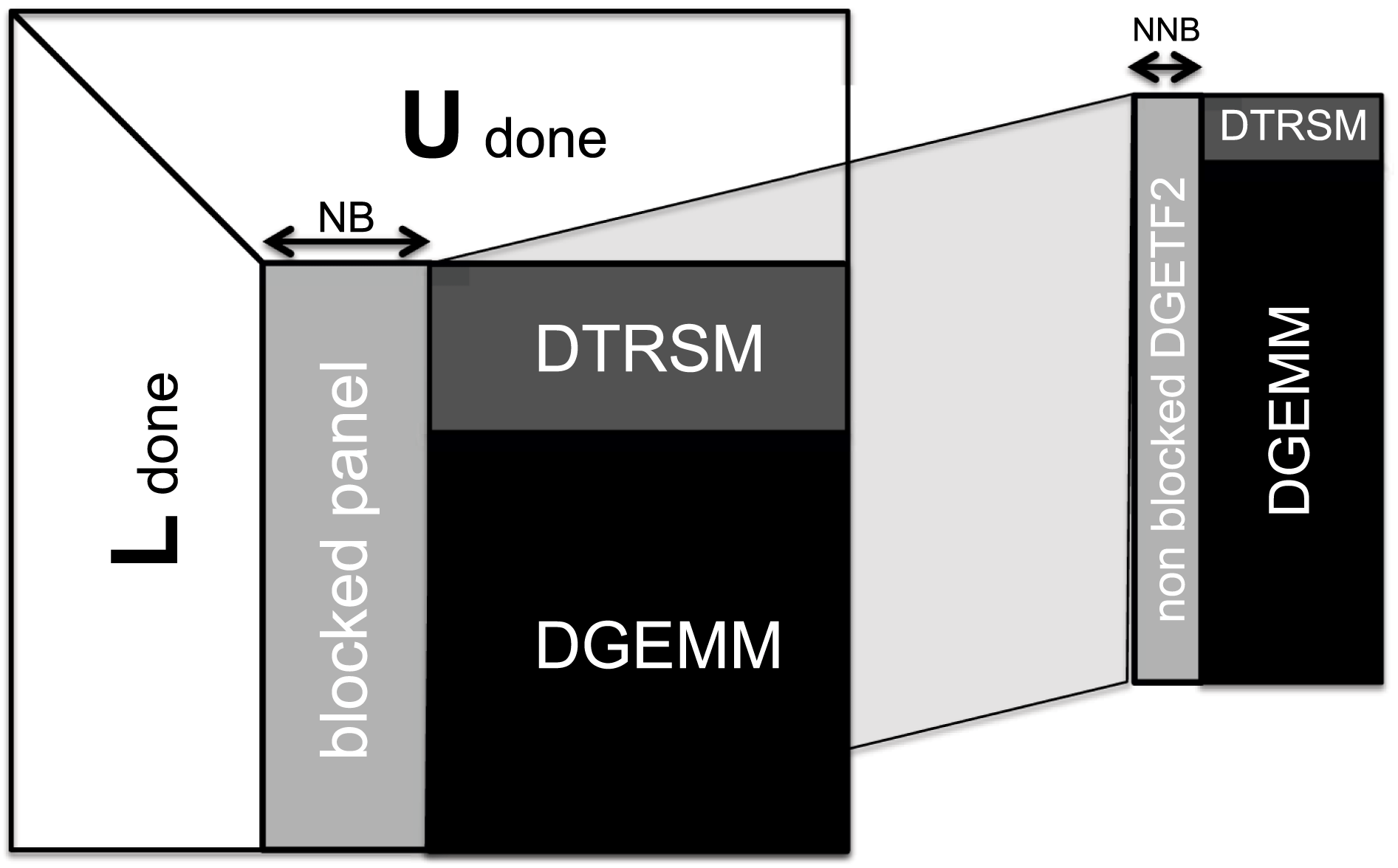
 $n_{b}$ columns (the panel) is factored and a pivoting pattern is produced (implemented by the DGETF2 routine). Then the elementary transformations, resulting from the panel factorization, are applied in a block fashion to the remaining part of the matrix (the trailing submatrix). This involves swapping up to
 $n_{b}$ rows of the trailing submatrix (DLASWP), according to the pivoting pattern, application of a triangular solve with multiple right-hand sides to the top
 $n_{b}$ rows of the trailing submatrix (DTRSM), and finally application of matrix multiplication of the form
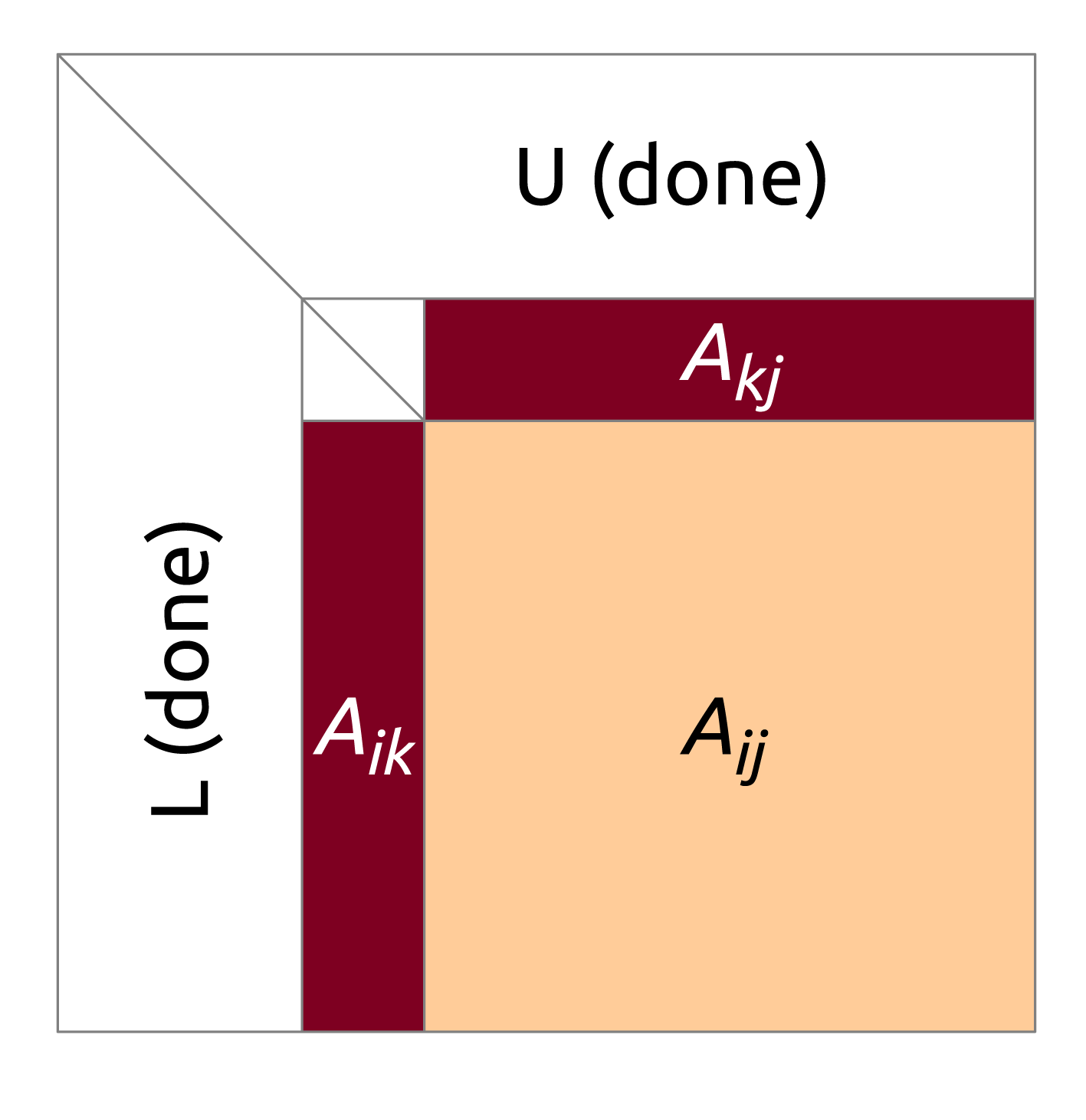
 $A_{ij}\leftarrow A_{ij}-A_{ik}\times A_{kj}$ (DGEMM), where
 $A_{ik}$ is the panel without the top
 $n_{b}$ rows,
 $A_{kj}$ is the top
 $n_{b}$ rows of the trailing submatrix, and
 $A_{ij}$ is the trailing submatrix without the top
 $n_{b}$ rows. Then the procedure is applied repeatedly, descending down the diagonal of the matrix: see Figure 4.1. The block algorithm is described in detail in section 2.6.3 of the book by Demmel (Reference Demmel1997).
The block LU factorization (Level 3 BLAS algorithm of LAPACK).
Instead of the Level 2 BLAS panel factorization (DGETF2) of LAPACK, we use a recursive partial pivoting panel factorization, which uses Level 3 BLAS operations. For a panel of  $k$ columns, the algorithm recursively factors the left
 $k/2$ columns, updates the right
 $k/2$ columns with DLASWP, DTRSM, and DGEMM, then recursively factors the right
 $k/2$ columns, and finally applies swaps to the left
 $k/2$ columns with DLASWP. The recursion terminates at a single column, where it simply searches for the maximum pivot, swaps elements, and scales the column by the pivot. Parallelism is introduced by splitting the panel into
 $p$ block rows, which are assigned to different processors.
4.1.2 Incremental pivoting
The most performance-limiting aspect of Gaussian elimination with partial pivoting is the panel factorization operation. First, it is an inefficient operation, usually based on a sequence of calls to Level 2 BLAS. Second, it introduces synchronization, by locking an entire panel of the matrix at a time. Therefore, it is desirable to split the panel factorization into a number of smaller, finer-granularity operations, which is the basic premise of the incremental pivoting implementation, also known in the literature as the tile LU factorization.
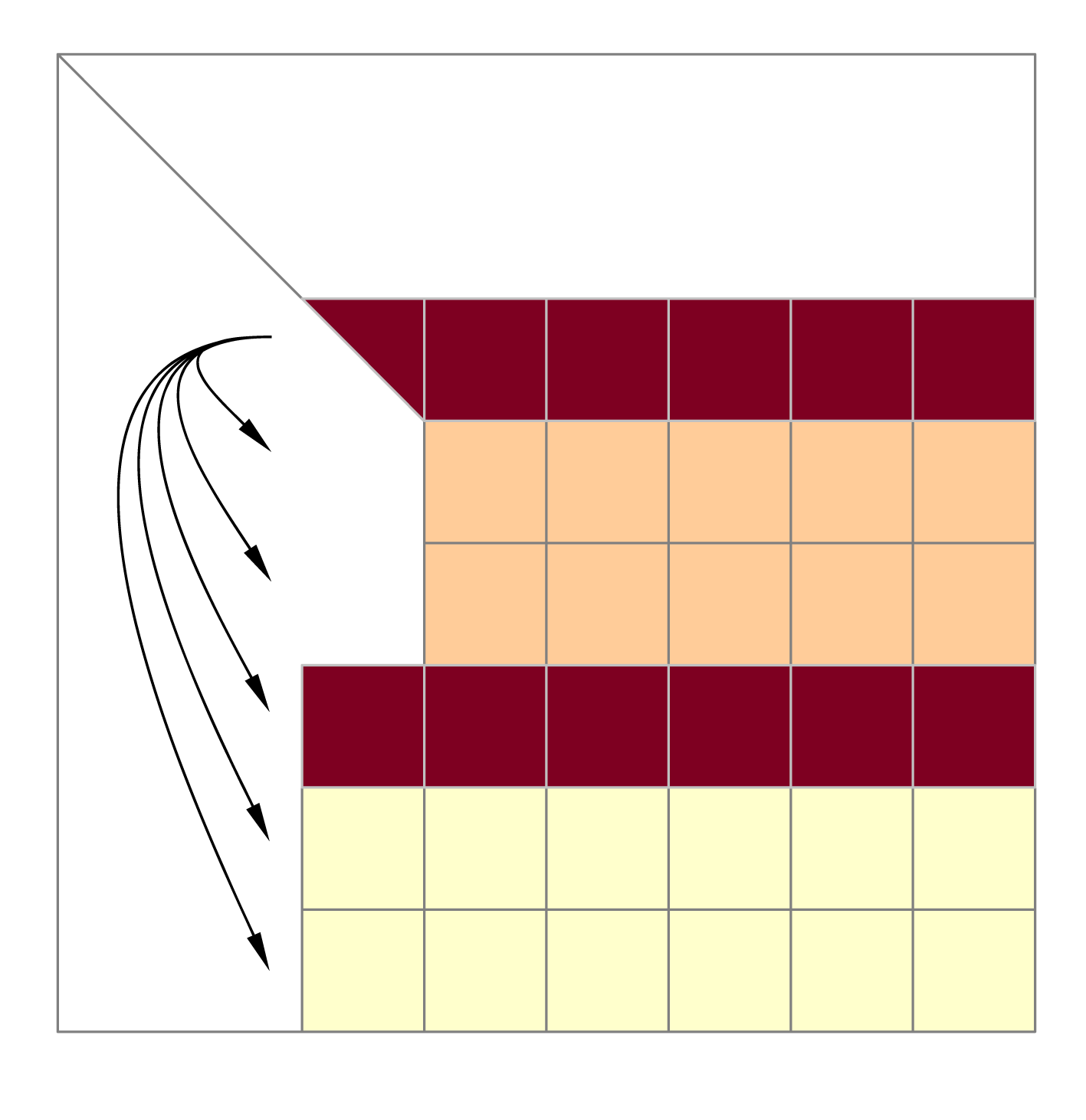
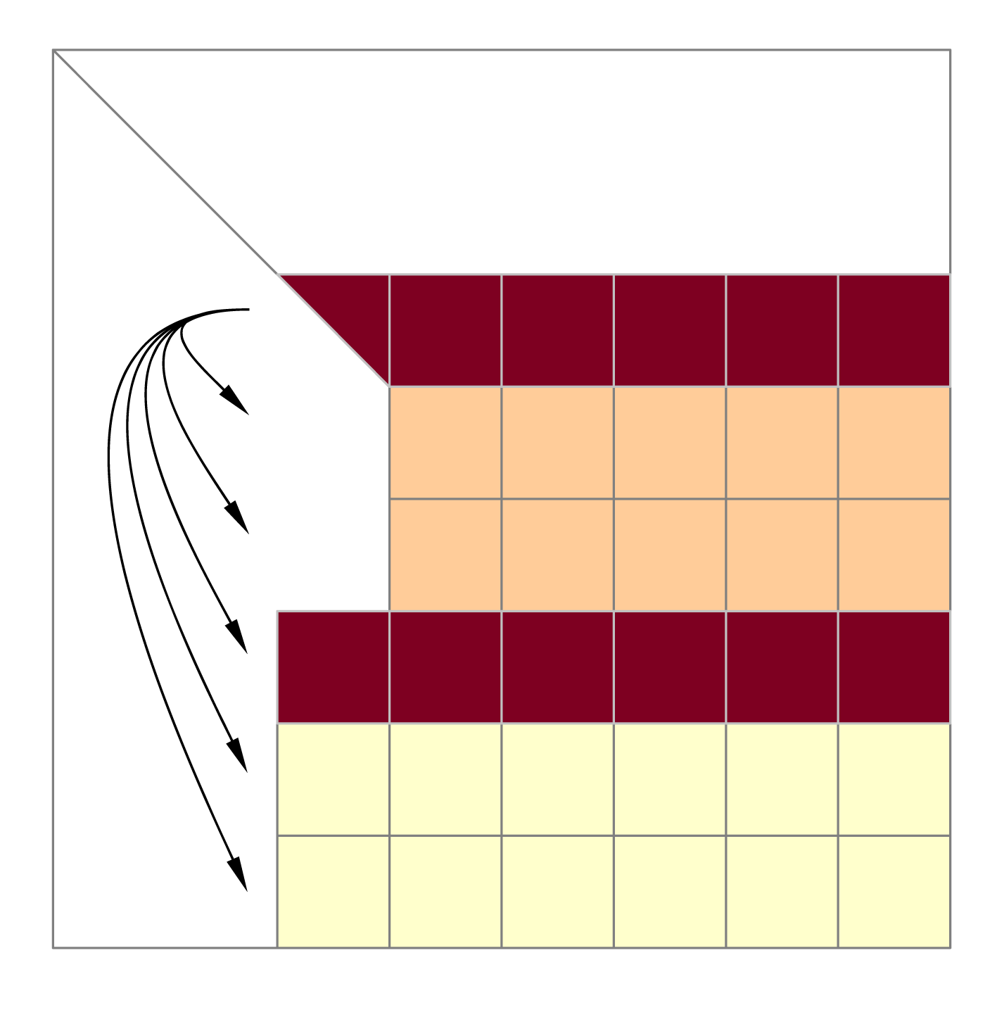
In this algorithm, instead of factoring the panel one column at a time, the panel is factored one tile at a time. The operation proceeds as follows. First the diagonal tile is factored using the standard LU factorization procedure. Then the factored tile is combined with the tile directly below it and factored. Then the refactored diagonal tile is combined with the next tile and factored again. The algorithm descends down the panel until the bottom of the matrix is reached. At each step, the standard partial pivoting procedure is applied to the tiles being factored. Also, at each step, all the tiles to the right of the panel are updated with the elementary transformations resulting from the panel operations: see Figure 4.2. This way of pivoting is basically the idea of pairwise pivoting applied at the level of tiles, rather than individual elements. The main benefit comes from the fact that updates of the trailing submatrix can proceed alongside panel factorizations, leading to a very efficient parallel execution, where multiple steps of the algorithm are smoothly pipelined.
Incremental LU factorization.
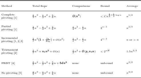
A straightforward implementation of incremental pivoting incurs more floating-point operations than partial pivoting. To reduce this additional cost, a second level of blocking, called inner blocking, is used within each tile (Joffrain, Quintana-Orti and van de Geijn Reference Joffrain, Quintana-Orti, van de Geijn, Dongarra, Madsen and Waśniewski2006, Buttari, Langou, Kurzak and Dongarra Reference Buttari, Langou, Kurzak and Dongarra2009). The total cost to factor an  $n\times n$ matrix is
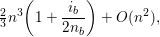 $$\begin{eqnarray}{\textstyle \frac{2}{3}}n^{3}\biggl(1+\frac{i_{b}}{2n_{b}}\biggr)+O(n^{2}),\end{eqnarray}$$
where  $n_{b}$ is the tile size and
 $i_{b}$ is the inner blocking size. A small value for
 $i_{b}$ decreases the flops but may hurt the efficiency of Level 3 BLAS operations, so
 $n_{b}$ and
 $i_{b}$ should be chosen to offer the best compromise between extra operations and BLAS efficiency.
With  $n_{b}=1$, incremental pivoting reduces to pairwise pivoting, hence the stability of incremental pivoting is assumed to be the same as pairwise pivoting (Joffrain et al. Reference Joffrain, Quintana-Orti, van de Geijn, Dongarra, Madsen and Waśniewski2006). For pairwise pivoting, the growth factor bound is
 $4^{n-1}$. Trefethen and Schreiber (Reference Trefethen and Schreiber1990) observed an average growth factor of
 $n$ for
 $n\leq 1024$, but more recently, Grigori, Demmel and Xiang (Reference Grigori, Demmel and Xiang2011) observed an average growth factor
 ${>}~n$ for
 $n\geq 4096$, leaving the question of stability open for large
 $n$.
4.1.3 Tournament pivoting
Classic approaches to the panel factorization with partial pivoting communicate asymptotically more than the established lower bounds (Demmel, Grigori, Hoemmen and Langou Reference Demmel, Grigori, Hoemmen and Langou2008a). The basic idea of communication-avoiding LU is to minimize communication by replacing the pivot search performed at each column with a block reduction of all the pivots together. This is done thanks to a new pivoting strategy referred to as tournament pivoting, which performs extra computations and is shown to be stable in practice. Tournament pivoting factors the panel in two steps. First, using a tournament selection, it identifies rows that can be used as good pivots for the factorization of the whole panel. Second, it swaps the selected pivot rows to the top of the panel, and then factors the entire panel without pivoting. With this strategy, the panel is efficiently parallelized, and the communication is provably minimized.
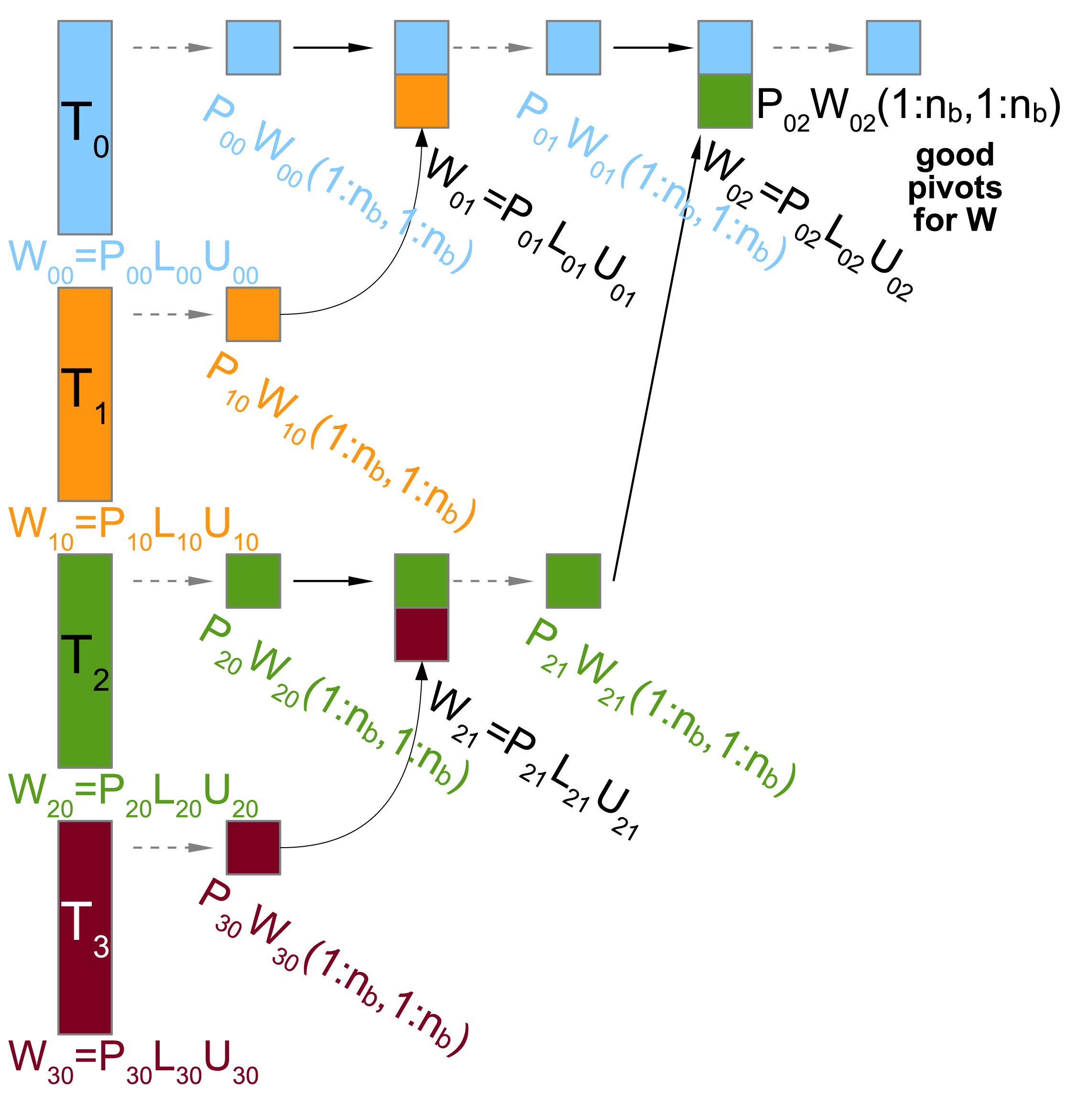
Figure 4.3 presents the first step of tournament pivoting for a panel  $W$ using a binary tree for the reduction operation. First, the panel is partitioned into
 $p_{r}$ blocks, that is,
 $W=[W_{00},W_{10},\ldots ,W_{p_{r}-1,0}]$, where
 $W_{ij}$ represents the block owned by thread
 $i$ at step
 $j$ of the reduction operation. Figure 4.3 shows an example with
 $p_{r}=4$.
Example of tournament pivoting with  $p_{r}=4$ processors, using a binary tree for the reduction operation.
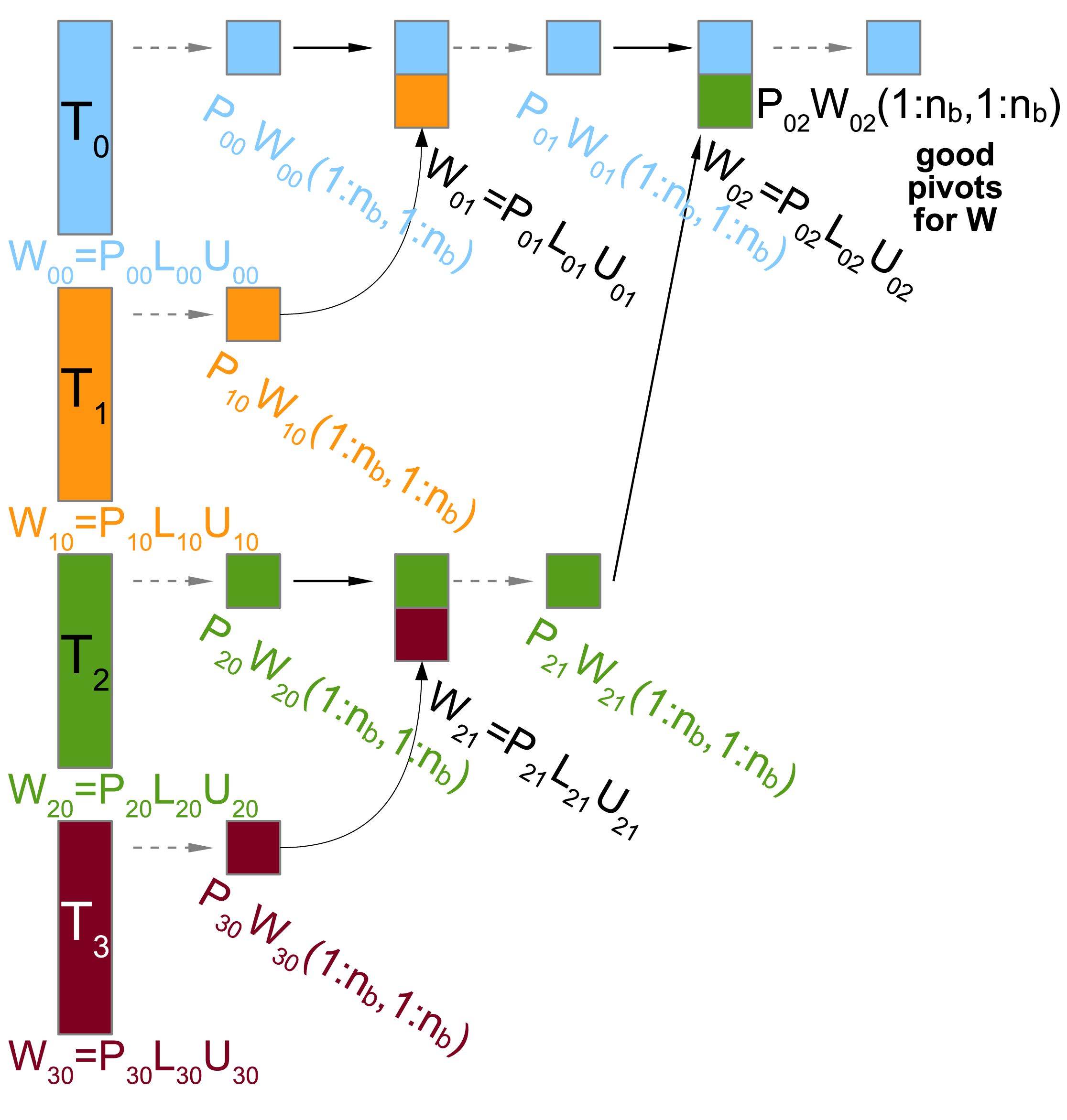
At the first step of the reduction operation, each thread,  $i$, applies Gaussian elimination with partial pivoting to its block,
 $W_{i0}$; then the resulting permutation matrix
 $P_{i0}$ is applied to the original unfactored block,
 $W_{i0}$, and the first
 $n_{b}$ rows of the permuted block
 $P_{i0}W_{i0}$ are selected as pivot candidates. These first pivot candidates represent the leaves of the reduction tree. At each node of the tree, the pivot candidates of two child nodes are merged on top of each other, and Gaussian elimination with partial pivoting is applied on the merged block. The resulting permutation matrix is then applied on the original unfactored merged block and the first
 $n_{b}$ rows are selected as new pivot candidates. By using a binary tree, this step is repeated
 $\log _{2}p_{r}$ times. The pivots obtained at the root of the tree are then considered to be good pivots for the whole panel. Once these pivots are permuted to the top of the panel, each thread applies Gaussian elimination without partial pivoting to its block,
 $W_{i0}$.
The example presented in Figure 4.3 uses a binary tree with two tiles reduced together at each level, but any reduction tree can be used, depending on the underlying architecture. The tournament pivoting implementation in PLASMA, used for experiments in this section, reduces four tiles at each level. This number of tiles is chosen because it gives a good ratio of kernel efficiency over one single core, relative to the time spent to perform the factorization of the subset.
For tournament pivoting, the best growth factor bound proved so far is  $2^{nH}$, where
 $H$ is the height of the reduction tree. With a binary tree,
 $H=\log _{2}p_{r}$, so the bound is
 $p_{r}^{n}$. However, Grigori et al. (Reference Grigori, Demmel and Xiang2011) have never observed a growth factor as large as
 $2^{n-1}$, even for pathological cases such as the Wilkinson matrix (Wilkinson Reference Wilkinson1988), and they conjecture that the upper bound is the same as partial pivoting,
 $2^{n-1}$. They observed an average growth factor of
 $1.5n^{2/3}$, independent of
 $p$. Our experiments in Section 4.2.3 confirm that tournament pivoting is as stable as partial pivoting in practice.
4.1.4 Random butterfly transform
As an alternative to pivoting, the partial random butterfly transformation (PRBT) preconditions the matrix as  $A_{r}=W^{T}\!AV$, such that, with probability close to 1, pivoting is unnecessary. This technique was proposed by Parker (Reference Parker1995b) and later adapted by Baboulin, Dongarra, Herrmann and Tomov (Reference Baboulin, Dongarra, Herrmann and Tomov2013) to reduce the computational cost of the transformation. An
 $n\times n$ butterfly matrix is defined as
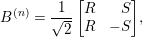 $$\begin{eqnarray}B^{(n)}=\frac{1}{\sqrt{2}}\left[\begin{array}{@{}cc@{}}R & \phantom{-}S\\ R & -S\end{array}\right]\!,\end{eqnarray}$$
where  $R$ and
 $S$ are random diagonal, non-singular matrices.
 $W$ and
 $V$ are recursive butterfly matrices of depth
 $d$, defined by
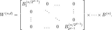 $$\begin{eqnarray}W^{(n,d)}=\left[\begin{array}{@{}cccc@{}}B_{1}^{(n/2^{d-1})} & 0 & \ldots \, & 0\\ 0 & \ddots & & \vdots \\ \vdots & & \ddots & 0\\ 0 & \ldots \, & 0 & B_{2^{d-1}}^{(n/2^{d-1})}\\ \end{array}\right]\times \cdots \times B^{(n)}.\end{eqnarray}$$
We use a depth  $d=2$, previously found to be sufficient in most cases (Baboulin et al. Reference Baboulin, Dongarra, Herrmann and Tomov2013). Since each
 $R$ and
 $S$ is diagonal,
 $W$ and
 $V$ can be stored as
 $n\times d$ arrays. Due to the regular sparsity pattern, multiplying an
 $m\times n$ matrix by
 $W$ and
 $V$ is an efficient,
 $O(dmn)$ operation.
After applying the PRBT, Gaussian elimination without pivoting is used to obtain the solution, as indicated in Algorithm 1.

While the randomization reduces the need for pivoting, the lack of pivoting can still be unstable, so we use iterative refinement to reduce the potential for instability. The cost of pivoting is thus avoided, at the expense of applying the PRBT and iterative refinement. As with no-pivoting LU, the growth factor remains unbounded. This can easily be seen by letting  $A=W^{-T}BV^{-1}$, where the first pivot,
 $b_{00}$, is zero. However, probabilistically no-pivoting LU (and hence PRBT) has been shown to have an average growth factor of
 $n^{3/2}$ (Yeung and Chan Reference Yeung and Chan1995).
4.1.5 No pivoting
This implementation of Gaussian elimination completely abandons pivoting. This can be done very rarely in practice without risking serious numerical consequences, or even a complete breakdown of the algorithm if a zero is encountered on the diagonal. In the following experiments, the implementation serves only as a performance baseline. Dropping pivoting increases performance for two reasons. First, the overhead of swapping matrix rows disappears. Second, the level of parallelism dramatically increases, since the panel operations now become parallel, and can also be pipelined with the updates to the trailing submatrix.
4.2 Experimental results
4.2.1 Hardware and software
The experiments were run on an Intel system with 16 cores and an AMD system with 48 cores. The Intel system has two sockets with 8-core Intel Sandy Bridge CPUs clocked at 2.6 GHz, with a theoretical peak of  $16~\text{cores}\times 2.6~\text{GHz}\times 8~\text{ops per cycle}\simeq 333~\text{Gflops}$ in double precision arithmetic. The AMD system has eight sockets with 6-core AMD Istanbul CPUs clocked at 2.8 GHz, with a theoretical peak of
 $48~\text{cores}\times 2.8~\text{GHz}\times 4~\text{ops per cycle}\simeq 538~\text{Gflops}$ in double precision arithmetic.
All presented LU codes were built using the PLASMA framework, relying on the CCRB tile layout and the QUARK dynamic scheduler. The GCC 4.1.2 compiler was used for compiling the software stack and Intel MKL (Composer XE 2013) was used to provide an optimized implementation of serial BLAS. On both systems, to avoid important variation in NUMA effects, the PLASMA framework relies on the hwloc library (Broquedis et al. Reference Broquedis, Clet-Ortega, Moreaud, Furmento, Goglin, Mercier, Thibault and Namyst2010) to efficiently bind the threads to cores located in multiple CPU sockets. And all experiments were run with the numactl command to distribute the data in a round-robin fashion over the NUMA locales of the machine. When the number of threads is insufficient to keep all sockets occupied then the memory pages are only bound to the NUMA locales with active PLASMA threads rather than the entire machine.
4.2.2 Performance
We now study the performance of our implementations on square random matrices in double real precision, and compare their performance with that of the LU factorization in MKL (DGETRF). While the absolute performance is different for single, single-complex, and double-complex precisions, we have observed trends similar to double precision for all precisions. In all cases, the matrix is initially in column-major layout, and we include the conversion to and from tiled layout in the time. Since each of our implementations uses a different pivoting strategy, we ran iterative refinement with all the algorithms to achieve the same level of accuracy, for a fair performance comparison. Namely, for MKL, we used the MKL iterative refinement routine DGERFS, while for the tile algorithms, we implemented a tiled iterative refinement with the same stopping criterion as that in DGERFS, that is, the iteration terminates when one of the following three criteria is satisfied.
1 The componentwise backward error,
 $\max _{i}|r_{i}|/(|A||\widehat{x}|+|b|)_{i}$, is less than or equal to $((n+1)\ast \mathbf{sfmin})/\mathbf{eps}$, where $r=A\widehat{x}-b$ is the residual vector and $\widehat{x}$ is the computed solution, $\mathbf{eps}$ is the relative machine precision, and $\mathbf{sfmin}$ is the smallest value such that $1/\mathbf{sfmin}$ does not overflow.
2 The componentwise backward error is not reduced by half.
3 The number of iterations is equal to ten.




For all of our experiments, iterative refinement converged in less than ten iterations. We observed that even with partial pivoting, it requires a couple of iterations to satisfy this stopping criterion (see Section 4.2.3). Furthermore, in many cases, the MKL version of DGERFS did not scale as well as our implementation. We suspect this is due to the need to compute  $|A||\widehat{x}|+|b|$ at each iteration.
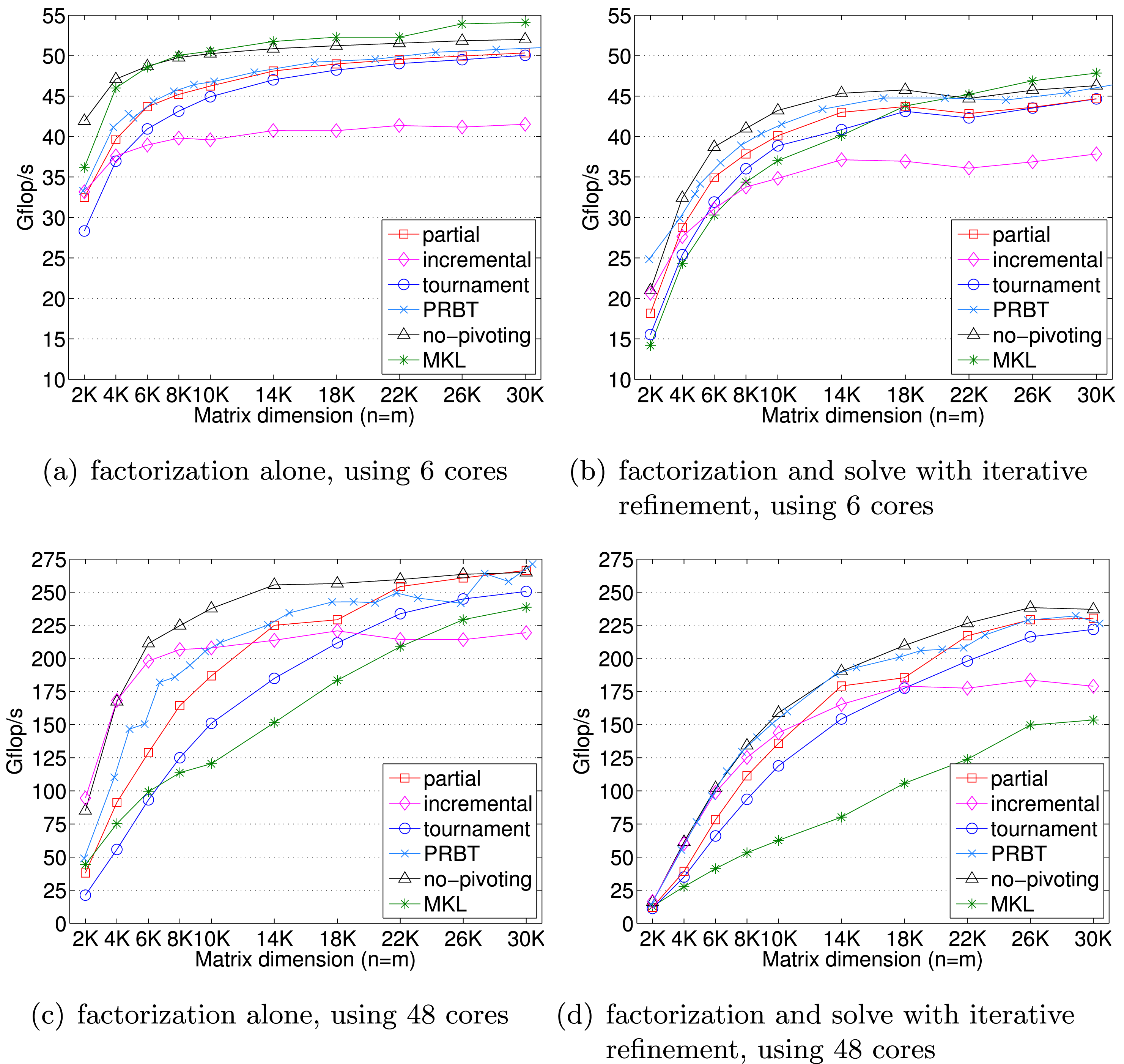
Asymptotic performance comparison of LU factorization algorithms on AMD Opteron.
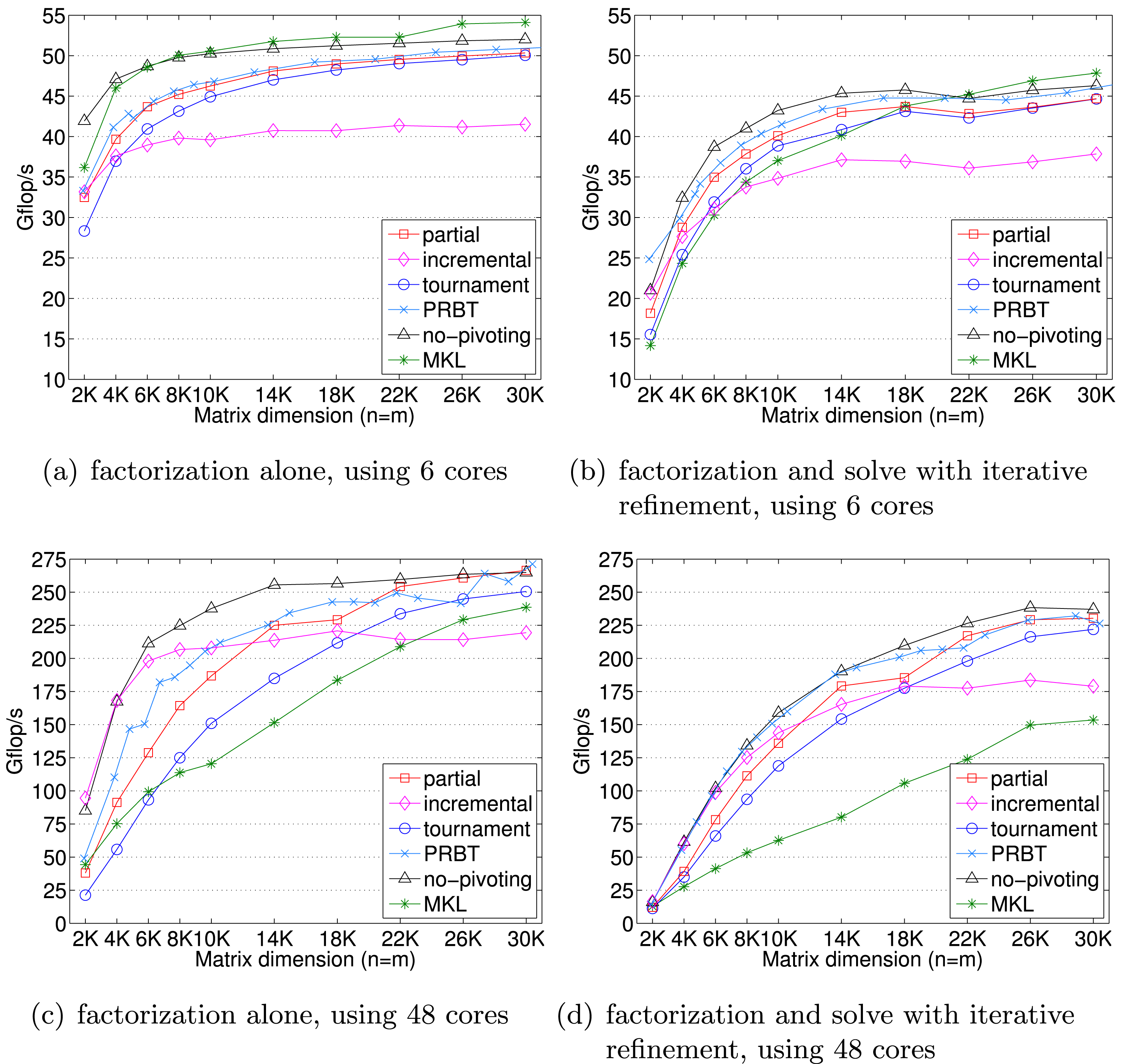
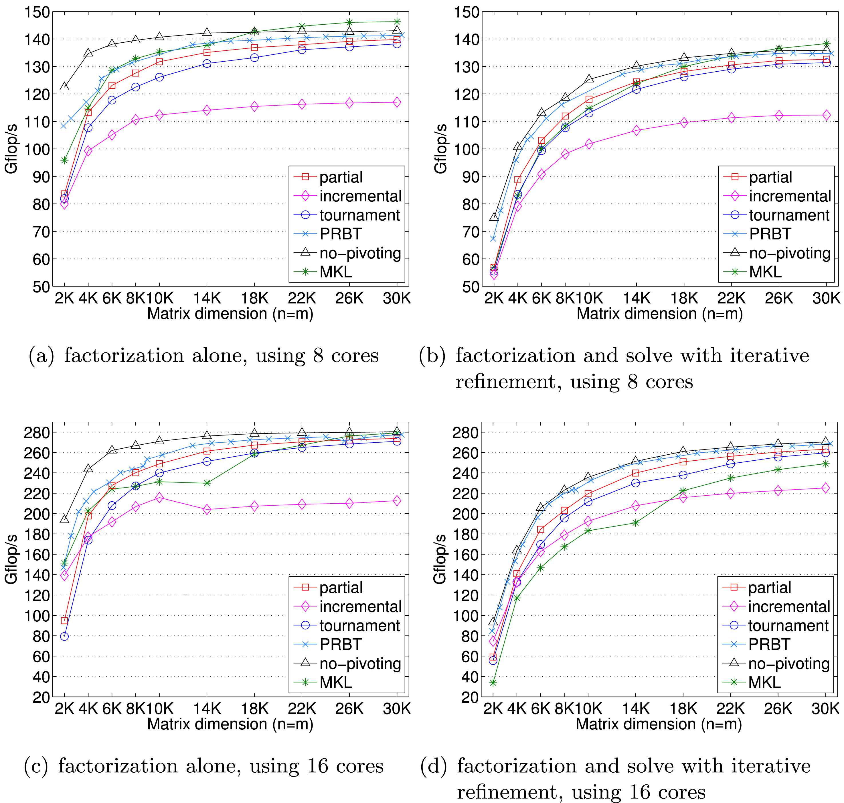
Asymptotic performance comparison of LU factorization algorithms on Intel Sandy Bridge.
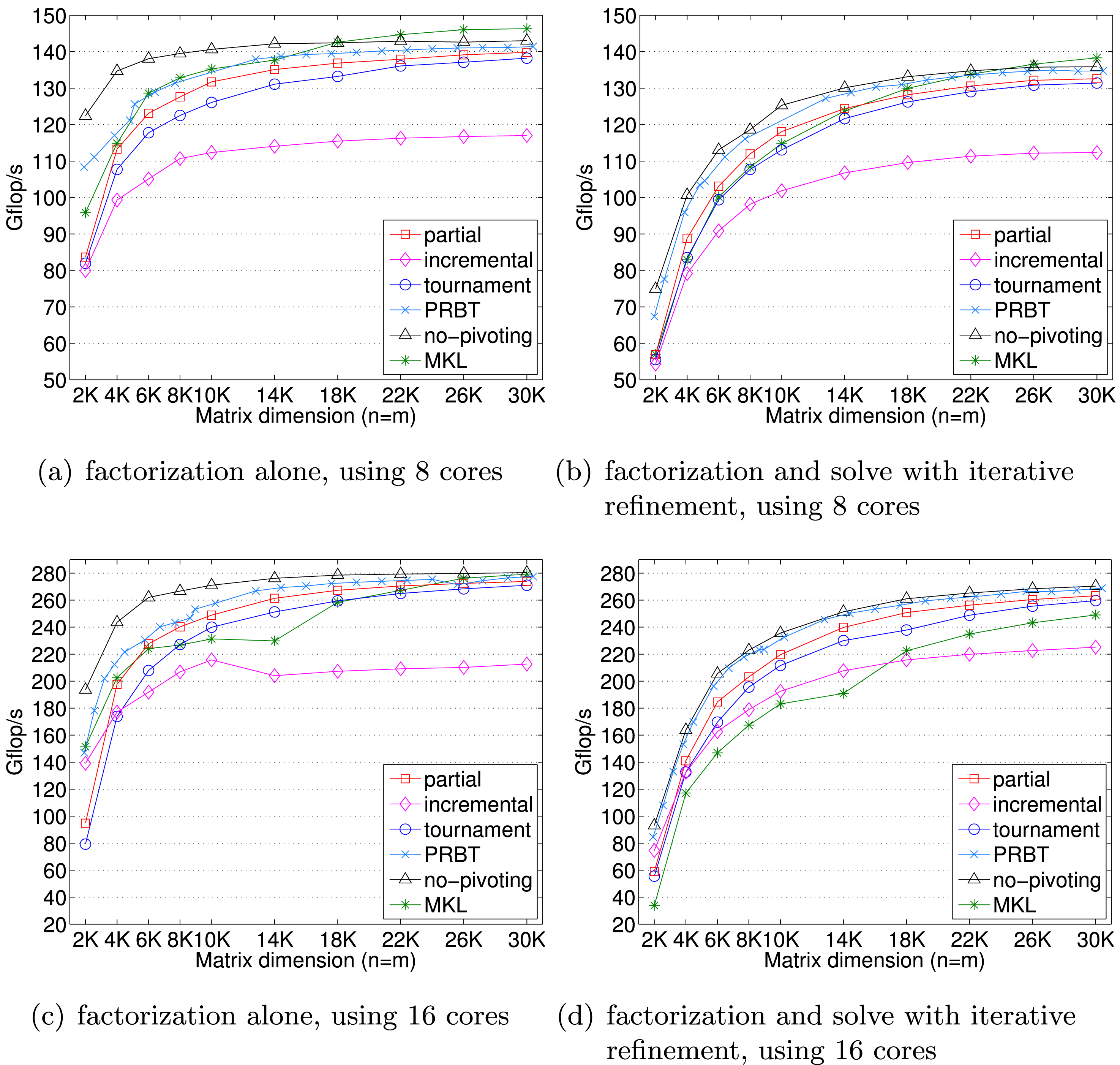
The performance of our implementations is sensitive to the tile size  $n_{b}$. Hence, for each matrix dimension
 $n$ on a different number of cores, we studied the performance of each algorithm with the tile sizes of
 $n_{b}=80$,
 $160$,
 $240$,
 $320$, and
 $400$. We observed that on
 $48$ cores of our AMD machine, the performance is especially sensitive to the tile size, and we tried the additional tile sizes of
 $n_{b}=340$,
 $360$, and
 $380$. In addition, the performance of our incremental pivoting is sensitive to the inner blocking size, and we tried using the block sizes of
 $i_{b}=10$,
 $20$, and
 $40$ for both
 $n_{b}=80$ and
 $160$;
 $i_{b}=10$,
 $20$,
 $30$,
 $40$,
 $60$, and
 $80$ for
 $n_{b}=240$; and
 $i_{b}=10$,
 $20$,
 $40$, and
 $80$ for both
 $n_{b}=320$ and
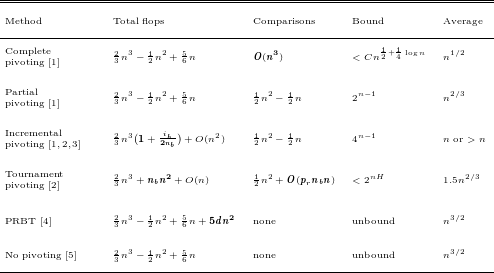
 $400$. Figures 4.4 and 4.5 show the performance obtained using the tile and block sizes that obtained the highest performance. For all algorithms, we compute the effective Gflops using the flops for partial pivoting, given in Table 4.1. For the solve with iterative refinement, we also include a pair of forward and backward substitutions,
 $2n^{2}$. For the tile algorithms, we included the data layout conversion time as a part of the solution time. We summarize our findings below.
Summary of floating-point operations (add, multiply, divide), floating-point comparisons, best known growth factor bound, and average-case growth factor. Differences in flops compared to partial pivoting are shown in bold. References: [1] Trefethen and Schreiber (Reference Trefethen and Schreiber1990); [2] Grigori et al. (Reference Grigori, Demmel and Xiang2011); [3] Buttari et al. (Reference Buttari, Langou, Kurzak and Dongarra2009); [4] Baboulin et al. (Reference Baboulin, Dongarra, Herrmann and Tomov2013); [5] Yeung and Chan (Reference Yeung and Chan1995).
∙ PRBT with the default transformation depth of two added only a small overhead over no-pivoting in all the test cases.
∙ In comparison to other pivoting strategies, incremental pivoting could exploit a large number of cores more effectively. As a result, when the performance is not dominated by the trailing submatrix updates (e.g. for a small matrix dimension on 48 cores), it obtained performance that is close to that of no-pivoting. However, for a large matrix dimension, due to the extra computation and special kernels required by incremental pivoting to update the trailing submatrix, its performance was lower than that of the partial or tournament pivoting LU that uses Level 3 BLAS DGEMM for their trailing submatrix updates.
∙ In comparison to MKL, our partial pivoting and tournament pivoting LU could effectively utilize a larger number of cores, as seen for medium-sized matrices on multiple sockets. This is probably a result of the extra parallelism attained by using a superscalar scheduler, as well as parallel panel factorizations.
∙ In this shared memory environment, partial pivoting outperformed tournament pivoting in all cases. However, this observation should not be extrapolated to distributed memory machines, where the communication latency becomes a significant part of the performance. There, the reduced communication in tournament pivoting may be more favourable.
∙ MKL performed well for large matrices, where the trailing submatrix update dominates the performance. Note that the combined cost for all the panels is
$O(n_{b}n^{2})$, compared to $O(n^{3})$ for the trailing submatrix update. Moreover, on a single socket, MKL outperformed no-pivoting for a sufficiently large matrix dimension. This could be because a tiled implementation loses efficiency due to the smaller BLAS kernels used during its trailing submatrix updates.∙ For small matrices, iterative refinement incurred a significant overhead, which diminishes for large matrices as the
$O(n^{3})$ factorization cost dominates the $O(n^{2})$ solve cost. The refinement overhead was particularly large for MKL, which we suspect is due to $|A||\widehat{x}|+|b|$ not being effectively parallelized in MKL.


4.2.3 Accuracy
To study the numerical behaviour of our implementations, we used the synthetic matrices from two recent papers (Grigori et al. Reference Grigori, Demmel and Xiang2011, Baboulin et al. Reference Baboulin, Dongarra, Herrmann and Tomov2013). We tested all these matrices, but here we present only a representative subset that demonstrates the numerical performance of the pivoting strategies. We also conducted the numerical experiments using all the matrix dimensions used in Section 4.2.2, but here we show only the results of  $n=30\,000$, which represent the numerical performance trends of the pivoting strategies for all other matrix dimensions. Table 4.2 shows some properties of these test matrices and the stability results of using partial pivoting. In the table, the second to sixth test matrices are from the paper by Grigori et al. (Reference Grigori, Demmel and Xiang2011), where the first two have relatively small condition numbers, while the rest are more ill-conditioned. The last three matrices are from the paper by Baboulin et al. (Reference Baboulin, Dongarra, Herrmann and Tomov2013), where the last test matrix gfpp is one of the pathological matrices that exhibit an exponential growth factor using partial pivoting. Since the condition number of the gfpp matrix increases rapidly with the matrix dimension, we used the matrix dimension of
 $m=1000$ for our study. Finally, incremental and tournament pivoting exhibit different numerical behaviour using different tile sizes. For the numerical results presented here, we used the tile and block sizes that obtain the best performance on the 16 core Intel Sandy Bridge. All the results are in double real precision.
Properties of test matrices and stability results of using partial pivoting  $(n=m=30\,000)$.
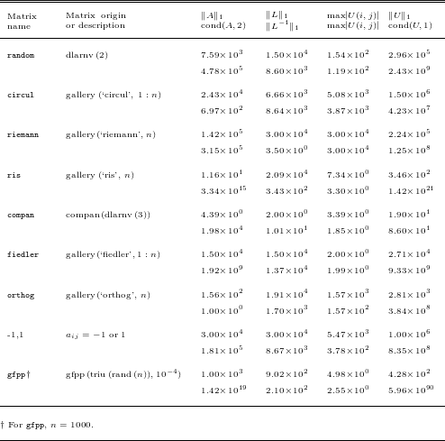
Numerical accuracy of LU factorization algorithms, showing error before refinement (top point of each line) and after each refinement iteration (subsequent points). Number of iterations is given at the bottom of (a); ‘F’ indicates failure (e.g. overflow).
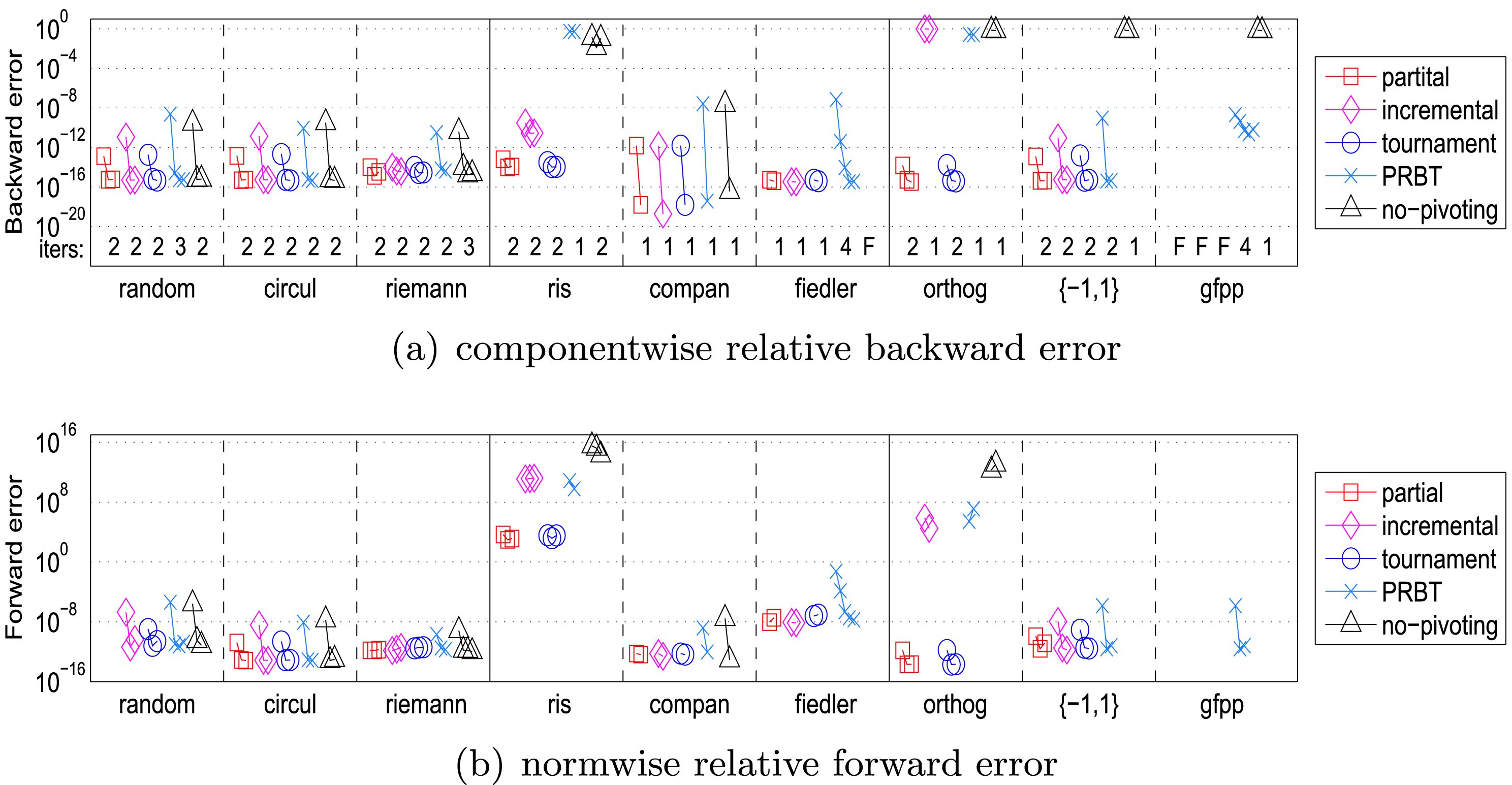
Figure 4.6(a) shows the componentwise backward errors,
 $$\begin{eqnarray}\max _{i}|r_{i}|/(|A||\widehat{x}|+|b|)_{i},\end{eqnarray}$$
at each step of iterative refinement. For these experiments, the right-hand side  $b$ is chosen such that the entries of the exact solution
 $x$ are uniformly distributed random numbers in the range of
 $[-0.5,0.5]$. We summarize our findings below.
∙ For all the test matrices, tournament pivoting obtained initial backward errors comparable to those of partial pivoting.
∙ No-pivoting was unstable for five of the test matrices (ris, fiedler, orthog, {-1,1}, and gfpp). For the rest of the test matrices, the initial backward errors of no-pivoting were significantly greater than those of partial pivoting, but were improved after a few refinement iterations.
∙ Incremental pivoting failed for the fiedler, orthog, and gfpp matrices. For other test matrices, its backward errors were greater than those of partial pivoting, but were improved to be of the same order as those of partial pivoting after a few refinement iterations. The only exception was with the ris matrix, where the refinement stagnated before reaching an accuracy similar to that of partial pivoting. In each column of the ris matrix, entries with smaller magnitudes are closer to the diagonal (i.e.
$a_{ij}=0.5/(n-i-j+1.5)$). As a result, the permutation matrix $P$ of partial pivoting has ones on the anti-diagonal.∙ When no-pivoting was successful, its backward errors were similar to those of PRBT. On the other hand, PRBT was more stable than no-pivoting, being able to obtain small backward errors for the fiedler, {-1,1}, and gfpp matrices.
∙ Partial pivoting was not stable for the pathological matrix gfpp. On the other hand, PRBT randomizes the original structure of the matrix and was able to compute the solution to reasonable accuracy. It is also possible to construct pathological test matrices where partial pivoting is unstable while tournament pivoting is stable, and vice versa (Grigori et al. Reference Grigori, Demmel and Xiang2011).


Figure 4.6(b) shows the relative forward error norms of our implementations, which were computed as  $\Vert x-\widehat{x}\Vert _{\infty }/\Vert x\Vert _{\infty }$. In the convergence of the forward error norms we observed similar trends to the backward errors. One difference was with the orthog test matrix, where iterative refinement could not adequately improve the forward errors of incremental pivoting and PRBT. Also, even though the backward errors of the ris test matrix were of the order of machine epsilon with partial and tournament pivoting, their relative forward errors were
 $O(1)$ due to the large condition number.
5 QR factorization
QR factorization is the most robust of the simple factorizations, but it comes at the cost of increased computational complexity of  $4/3n^{3}+O(n^{2})$ and slightly more complicated coding to account for exceptional floating-point behaviour that occurs for singular or numerically unbalanced matrices with entries spanning multiple magnitudes. QR’s robustness cannot be understated, however, as it is capable of handling singular and highly rank-deficient cases while still delivering useful numerical information about the input data; the only tool that could beat QR in that regard is SVD. A version of QR factorization can reveal the numerical rank of the input matrix if proper column pivoting is used, but this is beyond the scope of this paper.
The QR factorization of the matrix  $A$ is of the form
 $$\begin{eqnarray}A=QR,\end{eqnarray}$$
where  $Q$ is an
 $m\times m$ orthonormal matrix and
 $R$ is an
 $m\times n$ upper triangular matrix. LAPACK’s xGEQRF routine implements a right-looking QR factorization algorithm, whose first step consists of the following two phases. Here we use an obvious variant of the MATLAB colon notation.
1 Panel factorization. The first panel
$A_{:,1}$ is transformed into an upper triangular matrix.(a) xGEQR2 computes an
$m\times m$ Householder matrix $H_{1}$ such that and$$\begin{eqnarray}H_{1}^{T}A_{:,1}=\left(\begin{array}{@{}c@{}}R_{1,1}\\ 0\end{array}\right)\!,\end{eqnarray}$$$R_{1,1}$ is an $n_{b}\times n_{b}$ upper triangular matrix.(b) xLARFT computes a block representation of the transformation
$H_{1}$, that is,where$$\begin{eqnarray}H_{1}=I-V_{1}T_{1}V_{1}^{H},\end{eqnarray}$$$V_{1}$ is an $m\times n_{b}$ matrix and $T_{1}$ is an $n_{b}\times n_{b}$ upper triangular matrix.
2 Trailing submatrix update. xLARFB applies the transformation computed by xLARFT to the submatrix
$A_{:,2:n_{t}}$: $$\begin{eqnarray}\left(\begin{array}{@{}c@{}}R_{1,2:n_{t}}\\ \widehat{A}\end{array}\right):=(I-V_{1}T_{1}V_{1}^{H})\left(\begin{array}{@{}c@{}}A_{1,2:n_{t}}\\ A_{2:m_{t},2:n_{t}}\end{array}\right)\!.\end{eqnarray}$$


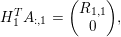





Then the QR factorization of  $A$ is computed by applying the same transformation to the submatrix
 $\widehat{A}$. The transformations
 $V_{j}$ are stored in the lower triangular part of
 $A$, while
 $R$ is stored in the upper triangular part. Additional
 $m\times n_{b}$ storage is required to store
 $T_{j}$.
A fine-grained algorithm for QR factorization (Buttari, Langou, Kurzak and Dongarra Reference Buttari, Langou, Kurzak and Dongarra2008b) requires restructuring of the above algorithm. The tiled QR factorization is constructed based on the following four elementary operations.
1 xGEQT2 performs the unblocked factorization of a diagonal block
$A_{kk}$ of size $n_{b}\times n_{b}$. This operation produces an upper triangular matrix $R_{kk}$, a unit lower triangular matrix $V_{kk}$ that contains $b$ Householder reflectors, and an upper triangular matrix $T_{kk}$ as defined by the ‘WY’ technique for accumulating the transformations (Bischof and Van Loan Reference Bischof and Van Loan1987, Schreiber and Van Loan Reference Schreiber and Van Loan1989). Note that both $R_{kk}$ and $V_{kk}$ can be written to the memory area that was used for $A_{kk}$, and thus no extra storage is needed; temporary workspace is needed to store $T_{kk}$. Further, where$$\begin{eqnarray}H_{1}H_{2}\ldots H_{b}=I-VTV^{T},\end{eqnarray}$$$V$ is an $n\times n_{b}$ matrix whose columns are the individual vectors $v_{1},v_{2},\ldots ,v_{b}$ associated with the Householder matrices $H_{1},H_{2},\ldots ,H_{b}$, and $T$ is an upper triangular matrix of order $n_{b}$.Thus, xGEQT2
$(A_{kk},T_{kk})$ performs $$\begin{eqnarray}A_{kk}\leftarrow V_{kk},R_{kk},\quad T_{kk}\leftarrow T_{kk}.\end{eqnarray}$$2 xLARFB applies the transformation
$(V_{kk},T_{kk})$ computed by subroutine xGEQT2 to a block $A_{kj}$.Thus, xLARFB
$(A_{kj},V_{kk},T_{kk})$ performs $$\begin{eqnarray}A\leftarrow (I-V_{kk}T_{kk}V_{kk}^{T})A_{kj}.\end{eqnarray}$$3 xTSQT2 performs the unblocked QR factorization of a matrix that is formed by coupling an upper triangular block
$R_{kk}$ with a square block $A_{ik}$. This subroutine will return an upper triangular matrix $\tilde{R}_{kk}$ which will overwrite $R_{kk}$ and $n_{b}$ Householder reflectors, where $n_{b}$ is the block size. Note that since $R_{kk}$ is upper triangular, the resulting Householder reflectors can be represented as an identity block $I$ on top of a square block $V_{ik}$. For this reason, no extra storage is needed for the Householder vectors since the identity block need not be stored, and $V_{ik}$ can overwrite $A_{ik}$. Also, a matrix $T_{ik}$ is produced for which storage space has to be allocated.Thus, xTSQT2
$(R_{kk},A_{ik},T_{ik})$ performs $$\begin{eqnarray}\left(\begin{array}{@{}c@{}}R_{kk}\\ A_{ik}\end{array}\right)\leftarrow \left(\begin{array}{@{}c@{}}I\\ V_{ik}\end{array}\right)\!,\tilde{R}_{kk},\quad T_{ik}\leftarrow T_{ik}.\end{eqnarray}$$4 xSSRFB applies the transformation computed by xTSQT2 to a matrix formed by coupling two square blocks
$A_{kj}$ and $A_{ij}$.Thus, xSSRFB
$(A_{kj},A_{ij},V_{ik},T_{ik})$ performs $$\begin{eqnarray}\left(\begin{array}{@{}c@{}}A_{kj}\\ A_{ij}\end{array}\right)\leftarrow \biggl(I-\left(\begin{array}{@{}c@{}}I\\ V_{ik}\end{array}\right)(T_{ik}\times V_{ik}^{T})\biggr)\left(\begin{array}{@{}c@{}}A_{kj}\\ A_{ij}\end{array}\right)\!.\end{eqnarray}$$




All of these elementary operations rely on BLAS subroutines to perform internal computations. They form the tiled QR algorithm shown in Algorithm 2.

Graphical representation of one iteration of the outer loop of the tiled QR algorithm with a matrix with  $3\times 3$ tiles.
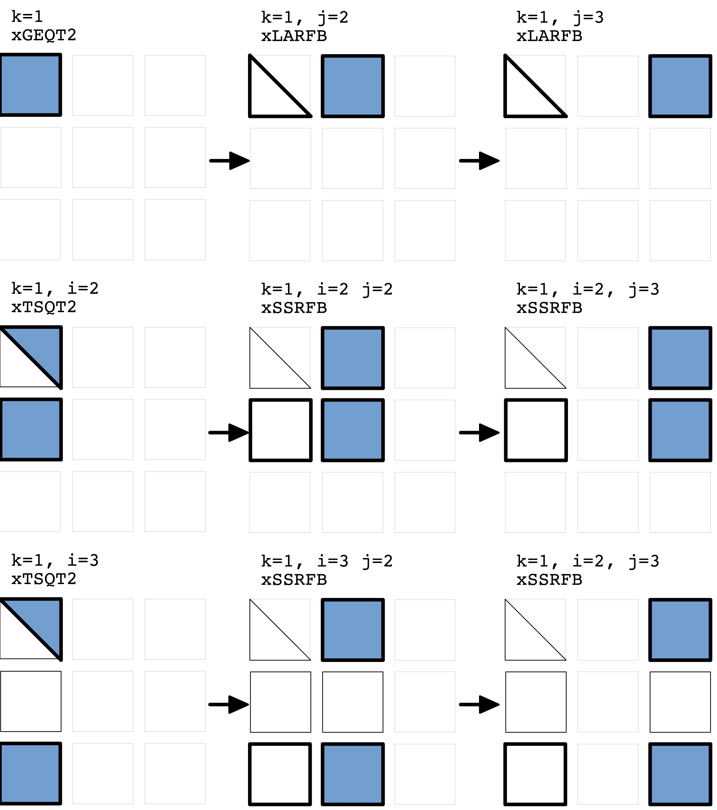
The operation count for Algorithm 2 is  $25\%$ higher than that of the LAPACK algorithm for QR factorization. More specifically, the tiled algorithm requires
 $5/2n^{2}(m-n/3)$ floating-point operations compared to the
 $4/2n^{2}(m-n/3)$ for the LAPACK algorithm. Details of the operation count of the parallel tiled algorithm are reported elsewhere (Buttari et al. Reference Buttari, Langou, Kurzak and Dongarra2008b).
Performance results demonstrate that it is worth paying this cost for the sake of increased parallelism and better scaling.
Figure 5.1 illustrates the data access to the tiles of a matrix for a single iteration (with  $k=1$) of the outer loop of Algorithm 2 with
 $p=q=3$. The thick borders indicate which blocks in the matrix are being read, and the shading indicates which blocks are being written to in the iteration. The
 $T_{kk}$ matrices are omitted in the figure for clarity.
There is a significant decrease of parallel efficiency which directly relates to the sequential nature of the panel factorization (Hadri, Ltaief, Agullo and Dongarra Reference Hadri, Ltaief, Agullo and Dongarra2010). Even though the panel itself (submatrices of width  $n_{b}$ below the diagonal) is tiled and executed in parallel with updates of the trailing submatrices when compared with LAPACK’s algorithm, the opportunities for parallelism across the panel are limited, which in turn generates load imbalance – especially when processing small or tall and narrow matrices whose size is
 $M\times N$ with
 $M\gg N$. For such matrices, a large portion of the elapsed time is spent in those sequential panel factorizations (Hadri, Ltaief, Agullo and Dongarra Reference Hadri, Ltaief, Agullo and Dongarra2009). Furthermore, the two-sided factorizations, such as SVD, that are based on bidiagonal reduction, require interleaved QR and LQ factorizations that are hindered by sequential panel processing for heavily off-square matrices (Ltaief, Luszczek, Haidar and Dongarra Reference Ltaief, Luszczek, Haidar, Dongarra, Wyrzykowski, Dongarra, Karczewski and Wasniewski2012).
6 Cholesky factorization
6.1 Algorithm for Cholesky factorization

Cholesky factorization (see Algorithm 3) is the fastest way to obtain triangular factors of a symmetric and/or Hermitian positive definitive matrix. The factors are either transposes or Hermitian transposes of each other and hence only one of them has to be stored: the choice of which determines whether  $LL^{T}$ or
 $U^{T}U$ formulation is used. For the most part, the factorization is immune to numerical round-off errors except for matrices that are close to being non-symmetric or indefinite, for which a slight perturbation can cause the factorization to fail due to a negative diagonal entry. In such cases, LDLT factorization will likely be more suitable.
The Cholesky factorization of a Hermitian positive definite matrix  $A$ is of the form
 $A=RR^{H}$, where
 $R$ is an
 $n\times n$ lower triangular matrix with positive real diagonals. The LAPACK routine xPOTRF computes the Cholesky factor
 $R$, whose
 $j$th step computes the
 $j$th block column
 $R_{j:n_{t},j}$ of
 $R$ in the following two phases.
1 Panel update. The
$j$th panel is updated using the previously computed columns of $R$:(a) xSYRK updates the diagonal block
$A_{j,j}$, $$\begin{eqnarray}A_{j,j}:=A_{j,j}-R_{j,1:(j-1)}R_{j,1:(j-1)}^{H};\end{eqnarray}$$(b) xGEMM updates the off-diagonal blocks,
$$\begin{eqnarray}A_{(j+1):n_{t},j}:=A_{(j+1):n_{t},j}-R_{(j+1):n_{t},1:(j-1)}R_{j,1:(j-1)}^{H}.\end{eqnarray}$$
2 Panel factorization. The
$j$th panel is factorized:(a) xPOTF2 computes the Cholesky factor
$R_{j,j}$ of $A_{j,j}$, $$\begin{eqnarray}A_{j,j}=R_{j,j}R_{j,j}^{H};\end{eqnarray}$$(b) xTRSM computes the off-diagonal blocks
$R_{(j+1):n_{t},j}$, $$\begin{eqnarray}R_{(j+1):n_{t},j}:=R_{j,j}^{-1}A_{(j+1):n_{t},j}.\end{eqnarray}$$






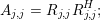


This is known as a left-looking algorithm, since the panel is updated at each step using the previous columns, which are on the left of the panel. If a right-looking algorithm is used, at each  $j$th step, the lower triangular part of the trailing matrix
 $A_{j:n_{t},j:n_{t}}$ is updated using xSYRK. When using multiple GPUs, xSYRK and xGEMM are called on each block column of
 $A_{j:n_{t},j:n_{t}}$. On the other hand, the left-looking algorithm accumulates all the updates to the panel into single calls to xSYRK and xGEMM, and exhibits more regular, and hence efficient, data access. The above algorithm references only the lower triangular part of
 $A$, which is overwritten by
 $R$. Alternatively, given the upper triangular part of
 $A$, xPOTRF can compute
 $R^{H}$ by block rows.
6.2 Supporting heterogeneous platforms
Ideally, our goal is a programming model that raises the level of abstraction above the hardware and its accompanying software stack to offer a uniform approach for algorithmic development and exploration of algorithmic variants. Below we describe the techniques we have developed in order to achieve an effective use of multi-way heterogeneous devices. Our techniques consider both the higher ratio of execution and the hierarchical memory model of new emerging accelerators and coprocessors.
GPU compute cards and multicore coprocessors, collectively known as hardware accelerators, have a very high computational peak compared to CPUs. Also, different types of accelerators have different capabilities, which makes it challenging to develop an algorithm that can achieve high performance and reach good scalability uniformly across the targeted platforms. From the hardware point of view, the accelerator communicates with the CPU using PCIexpress commands and DMA memory transfers, whereas from the software standpoint, the accelerator is a platform presented through a higher-level programming interface. The key features of our model are the processing unit capability (CPUs, GPUs, Xeon Phi), the memory access latency, and the communication cost. As with CPUs, the access time to the device memory for accelerators is slow compared to their peak performance. CPUs try to improve the effect of the long memory latency and scarce bandwidth by using hierarchical caches. This does not solve the slow memory problem completely, but is often effective for some workloads, and should be effective for Cholesky factorization as well. On the other hand, accelerators use massive multithreading operations to access large data sets that would overflow the size of most levels of cache. The often implemented solution involves having one of the accelerator’s hardware threads issue an access to the device memory, and then have that thread stalled until the memory is able to return the requested value. In the meantime, the accelerator’s scheduler switches to another hardware thread and continues executing that other thread. By doing this, the accelerator exploits parallelism inherent in the code in order to keep the functional units busy while the memory fulfils incoming requests. Compared to CPUs, which have limited memory channels and slower memory technology, the device memory delivers higher absolute bandwidth, for example, around 180 GB/s for a Xeon Phi and 160 GB/s for a Kepler K20c GPU, but also higher latency. To overcome the memory issues, the strategy we have developed prioritizes the data-intensive operations to be executed by the accelerator, and keeps the memory-bound kernels for the CPUs since the hierarchical caches with out-of-order superscalar scheduling are more appropriate for handling latency-sensitive codes. Moreover, in order to keep the accelerator busy, we have redesigned the kernels and proposed dynamically guided data distribution to exploit enough parallelism to keep the accelerators and CPUs busy.

From the point of view of the programming model, there has to be a distinction between the two levels of parallelism. We thus convert each algorithm into a host part and an accelerator part. Each routine that is to be run on the accelerator must be extracted into a separate kernel function – specific to the hardware. The kernel function itself may have to be carefully optimized for the accelerator, which includes unrolling the loops, replacing some memory-bound operations with compute-intensive ones, even if it incurs an extra cost. Also, arranging the tasks to use the device memory efficiently should be included. The host code must manage the device memory allocation, the CPU-accelerator data movement, and the kernel invocation. We redesigned our QUARK runtime engine in order to present a much easier programming environment and to simplify scheduling. This often allows us to maintain a single source version that handles different types of accelerators either independently or even when mixed together. Our intention is that our model simplifies most of the hardware details, but at the same time gives the user finer levels of control. Algorithm 4 shows the pseudocode for the Cholesky factorization, as an algorithm designer sees it, with much more low-level language detail when compared with Algorithm 3. The code consists of a sequential part that is simple to comprehend and independent of the architecture. Each of these sequential calls represents a task that is passed to the scheduler, which stores it for later execution, when all of the task’s dependencies are satisfied. Each task consists of a call to a kernel function that could either be a CPU or an accelerator code. For the most part, we hid the differences between hardware and let the QUARK scheduler handle the transfer of data on behalf of the user. In addition, we developed low-level optimizations for the accelerators in order to accommodate hardware- and library-specific tuning and requirements. Moreover, we implemented a set of directives that are evaluated at runtime in order to fully map the algorithm to the hardware and execute at a rate that is close to the peak performance of the system. Using these strategies, we can more easily develop simple and portable code that can run on different heterogeneous architectures and let the scheduling and execution runtime do the majority of the tedious bookkeeping.
6.3 Resource capability weights
To simplify expression of linear algebra algorithms, we would like to find a simple way of accounting for the differences in the computing capability of the user’s CPUs and accelerators. Clearly, it is not possible to balance the load perfectly for every run in the presence of operating system overhead. However, we could treat the computing devices as equivalent peers and assign them an equivalent amount of work. Such a naïve strategy would obviously cause the accelerators to be under-utilized and would render them mostly idle. As mentioned above, we propose, as our design principle, to assign the latency-bound operations to the CPUs and the compute-intensive operations to the accelerators. In order to support multi-way heterogeneous hardware, the QUARK scheduler was extended with a mechanism for distributing tasks based on the individual capabilities of each device. For each device  $i$ and each kernel type
 $k$, QUARK maintains an
 ${\it\alpha}_{i,k}$ parameter which corresponds to the effective performance rate that can be achieved on that device. In the context of linear algebra algorithms, this means that we need an estimation of performance for Level 1, 2, and 3 BLAS operations. This can be done by the developer during the implementation, where the user gives directives to QUARK to indicate whether a given kernel is a bandwidth-bound or a compute-bound function. This is shown in Algorithm 4, with a call to Task_Flag_Set with a BLAS2 argument. Also, an estimate of the volume of data and the elapsed time of the kernel is needed for the QUARK scheduler.
We can improve this further by fully utilizing all of the available resources – in particular, by exploiting the idle time of the CPUs that are often fast enough to handle more work in addition to the latency-bound tasks. Based on the parameters defined above, we can compute resource capability weights for each of the tasks, and they will reflect the cost of executing them on a specific device. This cost is primarily based on the communication cost of moving the data and on the type of computation performed by the task – either memory-bound or compute-bound. For a task that requires an  $n\times n$ data, we define its computation type to be from one of the levels of BLAS (either 1, 2 or 3). Thus the two factors are fairly simply defined as
 $$\begin{eqnarray}\displaystyle \text{communication} & = & \displaystyle \frac{n\times n}{\text{bandwidth}},\nonumber\\ \displaystyle \text{computation} & = & \displaystyle n^{k}\times {\it\alpha}_{ik}\quad \text{where }k\text{ is Level }k\text{ BLAS}.\nonumber\end{eqnarray}$$
The resource capability weights for a task are then the ratio of the total cost of executing the task on one resource versus the cost of doing it on another resource. For example, the resource capability weights for the update operation – a Level 3 BLAS – is around  $1:10$, which means that the GPU can execute
 $10\times$ as many update tasks as the CPU can.
Each task is created at runtime and presented to the scheduler, which then assigns it to the resource with the largest remaining capability weight. This greedy heuristic takes into account the weights of the resource, as well as the current number of waiting tasks preferred to be executed by this resource. For example, for the CPU, the panel tasks are memory-bound and thus executing them on the CPU is always preferred. This heuristic tries to maintain constant ratios of the capability weights across all the resources.
When using multiple accelerators, the data is initially distributed over all the accelerators in a one-dimensional block cyclic fashion, with an approximately equal number of columns assigned to each. Note that the data are allocated on each device as one contiguous memory block, with the data being distributed as columns within the contiguous memory segment. This contiguous data layout allows large update operations to take place over a number of columns via a single Level 3 BLAS operation, which is far more efficient than having multiple calls with block columns.
Experimentally, the standard and uniform one-dimensional block cyclic data layout may hinder performance in heterogeneous multi-accelerator environments (Haidar et al. Reference Haidar, Cao, Yarkhan, Luszczek, Tomov, Kabir and Dongarra2014a). The execution flow becomes bound by the performance of the slowest machine. What is needed is an adjustment to the data distribution that takes into account the resource capability weights thus resulting in hardware-guide data distribution (HGDD). Using the QUARK runtime, the data is either distributed or redistributed in an automatic fashion so that each device gets the appropriate volume of data to match its capabilities.
Performance scalability of Cholesky factorization on multicore CPU and multiple accelerators (up to six NVIDIA Kepler K20c GPUs).
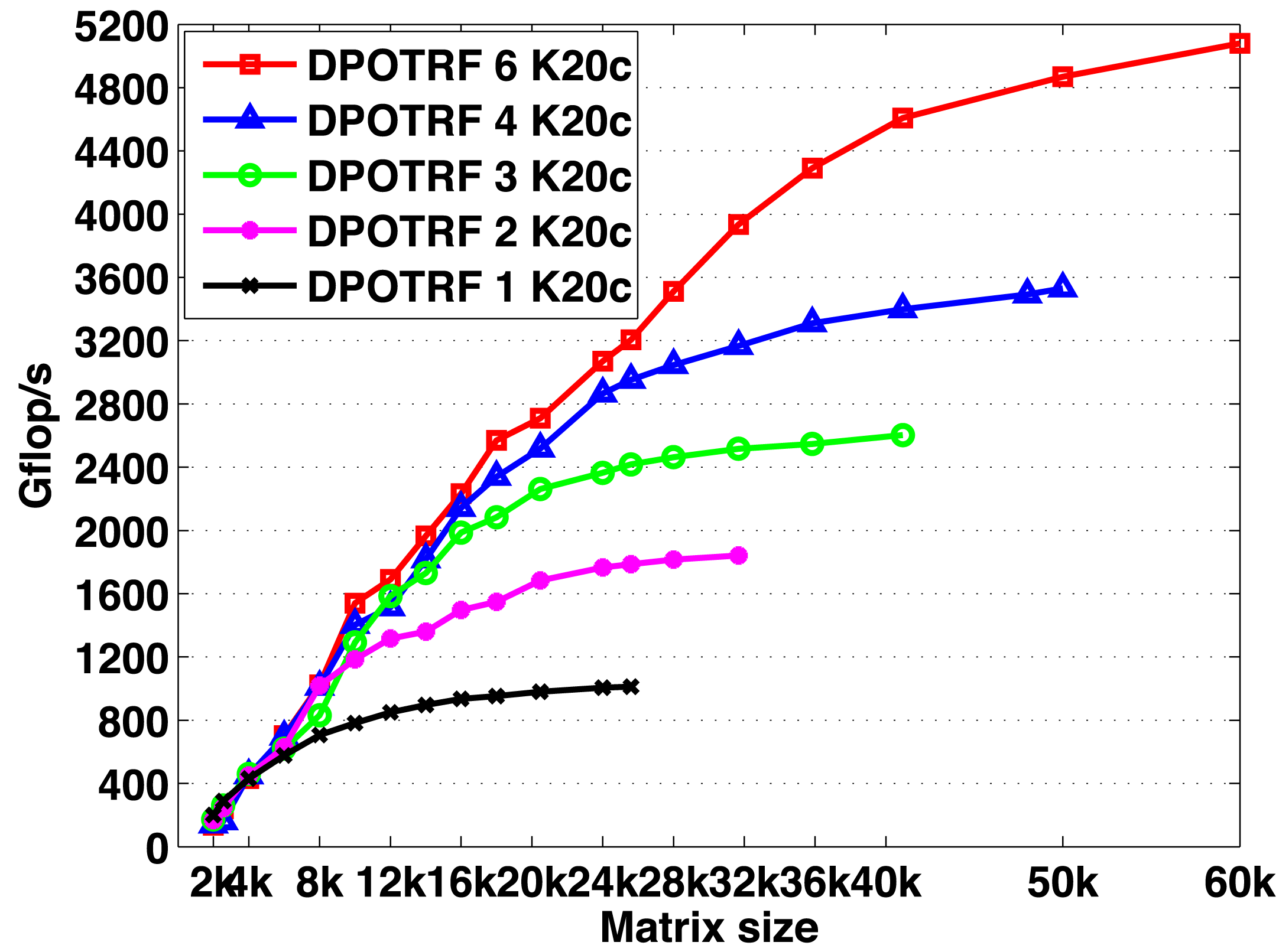
Performance scalability of Cholesky factorization on multicore CPU and multiple accelerators (up to three Xeon Phi accelerators).
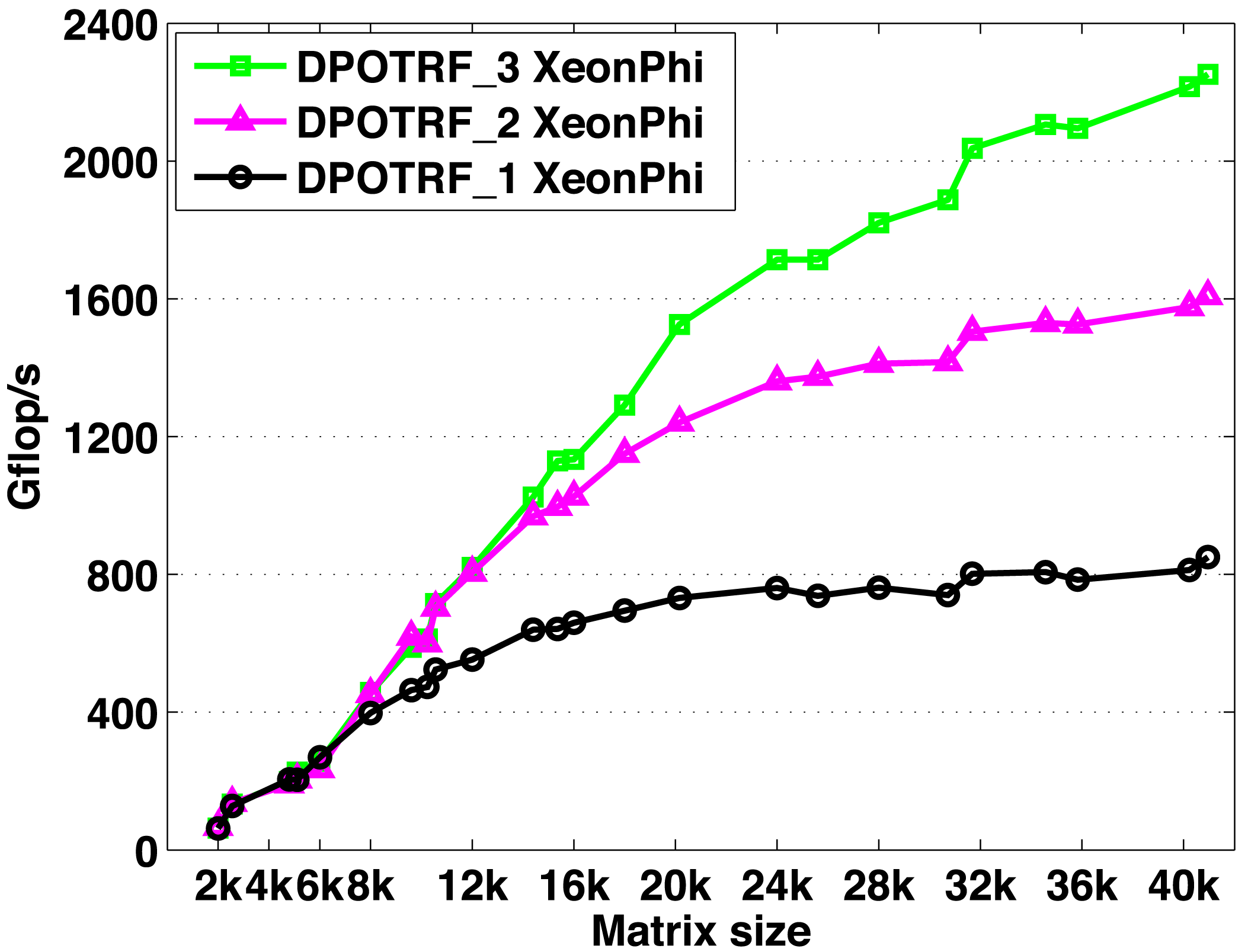
Figures 6.1 and 6.2 show the performance scalability of the Cholesky factorization in double precision on either six NVIDIA GPUs or three Intel Xeon Phi accelerators, respectively. The curves show performance in terms of Gflops, and we note that this also reflects the elapsed time (i.e., for a matrix of a given size, performance that is  $2\times$ higher corresponds to an elapsed time that is
 $2\times$ shorter). Our heterogeneous multi-device implementation shows very good scalability on both systems. For a
 $60\times 10^{3}$ matrix, the Cholesky factorization achieves over
 $5100$ Gflops when using the six NVIDIA Kepler K20c GPUs. We observe similar performance and scalability trends when using the other system, and for a matrix of size
 $40\times 10^{3}$, the Cholesky factorization reaches up to
 $2300$ Gflops when using the three Intel Xeon Phi coprocessors.
7 LDLT decomposition
A symmetric matrix  $A$ is called indefinite when its quadratic form
 $x^{T}Ax$ can take both positive and negative values. Dense linear systems of equations,
 $Ax=b$, with a symmetric indefinite coefficient matrix
 $A$, appear in many studies of physics, including physics of structures, acoustics, and electromagnetism. For instance, such systems arise in the linear least-squares problem for solving an augmented system (Björck Reference Björck1996, p. 77), or in electromagnetism, where the discretization by the boundary element method results in linear systems with dense complex symmetric (non-Hermitian) matrices (Nédélec Reference Nédélec2001). However, it is a challenge to develop an efficient or scalable symmetric indefinite factorization algorithm that takes advantage of the symmetry and has a provable numerical stability. The main reason for this is that stable factorization requires pivoting, which is difficult to implement and parallelize efficiently on current hardware architectures. In this section, we discuss our efforts to overcome these challenges.
7.1 Implementation on multicore CPUs
7.1.1 LAPACK: Bunch–Kaufman algorithm
For solving a symmetric indefinite linear system, LAPACK implements a partitioned LDL $^{\text{T}}$factorization with the Bunch–Kaufman algorithm (Bunch and Kaufman Reference Bunch and Kaufman1977, Anderson and Dongarra Reference Anderson and Dongarra1989) that computes
 $$\begin{eqnarray}PAP^{T}=LDL^{T},\end{eqnarray}$$
where  $D$ is a block-diagonal matrix with either
 $1\times 1$ or
 $2\times 2$ diagonal blocks. This algorithm is backward stable, subject to growth factors (Ashcraft, Grimes and Lewis Reference Ashcraft, Grimes and Lewis1998), and performs about
 $\frac{1}{3}n^{3}+O(n^{2})$ flops; see Algorithm 5.

To select the pivot at each step of the panel factorization, the algorithm scans two columns of the trailing submatrix, and depending on the numerical values of the scanned matrix entries, it uses either a  $1\times 1$ or
 $2\times 2$ pivot. This results in synchronizations and irregular data access (due to the symmetric matrix storage), which have become expensive on modern computers. As a result, in many cases, the implementation of the algorithm cannot obtain high performance or exploit parallelism.
7.1.2 PLASMA: random butterfly transformation
PLASMA provides a set of dense linear algebra routines based on tiled algorithms that break a given algorithm into fine-grained computational tasks that operate on small square submatrices called tiles. Since each tile is stored contiguously in memory and fits in a local cache memory, this algorithm can take advantage of the hierarchical memory architecture used in modern computing hardware. Furthermore, by dynamically scheduling the tasks as soon as all of their dependencies are resolved, PLASMA can exploit a fine-grained parallelism and utilize a large number of cores.
Randomized algorithms are gaining popularity in linear algebra since they can often exploit more parallelism than corresponding deterministic algorithms (Parker Reference Parker1995a). To solve a symmetric indefinite linear system, PLASMAextends a randomization technique developed for the LU factorization (Baboulin et al. Reference Baboulin, Dongarra, Herrmann and Tomov2013) to symmetric indefinite systems (Becker, Baboulin and Dongarra Reference Becker, Baboulin, Dongarra, Wyrzykowski, Dongarra, Karczewski and Wasniewski2012, Baboulin, Becker and Dongarra Reference Baboulin, Becker and Dongarra2012). That is, it uses a multiplicative preconditioner by means of random matrices called recursive butterfly matrices  $U_{k}$:
 $$\begin{eqnarray}(U_{d}^{T}U_{d-1}^{T}\ldots U_{1}^{T})A(U_{1}U_{2}\ldots U_{d}),\end{eqnarray}$$
where
 $$\begin{eqnarray}U_{k}=\left(\begin{array}{@{}ccc@{}}B_{1} & & \\ & \ddots & \\ & & B_{2^{k-1}}\end{array}\right)\!,\quad B_{k}=\frac{1}{\sqrt{2}}\left(\begin{array}{@{}cc@{}}R_{k} & S_{k}\\ R_{k} & -S_{k}\end{array}\right)\!,\end{eqnarray}$$
and  $R_{k}$ and
 $S_{k}$ are random diagonal matrices. As a result, the original matrix
 $A$ is transformed into a matrix that is sufficiently random so that, with probability close to one, pivoting is not needed.
This random butterfly transformation (RBT) requires only  $2dn^{2}+O(n)$ flops compared to the
 $\frac{1}{3}n^{3}+O(n^{2})$ flops required for the factorization. In practice,
 $d=2$ achieves satisfying accuracy, and this is the default setup used in PLASMA. Since
 $A$ is factorized without pivoting after RBT, it allows a scalable factorization of a dense symmetric indefinite matrix.
The main drawback of this method is reliability. There is no theory demonstrating its deterministic stability. Though it may fail in certain cases, numerical tests showed that with iterative refinement, it is reliable for many test cases, including pathological ones (Becker et al. Reference Becker, Baboulin, Dongarra, Wyrzykowski, Dongarra, Karczewski and Wasniewski2012). Furthermore, since iterative refinement is required, the failure of the method can be signalled without extra computation.
7.1.3 PLASMA: Aasen’s algorithm
To solve a symmetric indefinite linear system, Aasen’s algorithm (Aasen Reference Aasen1971) factorizes  $A$ into an LTL
 $^{\text{T}}$decomposition of the form
 $$\begin{eqnarray}PAP^{T}=LTL^{T},\end{eqnarray}$$
where  $P$ is a permutation matrix,
 $L$ is a unit lower triangular matrix, and
 $T$ is a symmetric tridiagonal matrix; see Algorithm 6. Aasen’s algorithm takes advantage of the symmetry in
 $A$ and performs
 $\frac{1}{3}n^{3}+O(n^{2})$ flops, which is a half of the flops needed for an LU factorization of
 $A$, and the same as the number of the flops required by the Bunch–Kaufman algorithm. Furthermore, it is backward stable and subject to a growth factor. Once the factorization is computed, the solution
 $x$ is computed by successively solving the linear systems with the matrices
 $L$,
 $T$, and
 $L^{T}$.

To exploit the memory hierarchy on a modern computer, a partitioned version of Aasen’s algorithm was proposed (Rozloz̆ník, Shklarski and Toledo Reference Rozloz̆ník, Shklarski and Toledo2011). This algorithm first factorizes a panel in a left-looking fashion, and then uses Level 3 BLAS operations to update the trailing submatrix in a right-looking way. Compared to a standard column-wise algorithm, this partitioned algorithm slightly increases the operation count, performing
 $$\begin{eqnarray}\frac{1}{3}\biggl(1+\frac{1}{n_{b}}\biggr)n^{3}+O(n^{2}n_{b})\end{eqnarray}$$
flops with a block size of  $n_{b}$. However, Level 3 BLAS can be used to perform most of these flops; i.e.,
 $$\begin{eqnarray}\frac{1}{3}\biggl(1+\frac{1}{n_{b}}\biggr)n^{3}\end{eqnarray}$$
flops. Since the Level 3 BLAS operations have higher ratios of flop counts over communication volumes than the Level 2 BLAS or Level 1 BLAS operations do, this partitioned algorithm is shown to significantly shorten the factorization time on modern computers, where data transfer is much more expensive than floating-point operations (Rozloz̆ník et al. Reference Rozloz̆ník, Shklarski and Toledo2011). A serial implementation of the partitioned Aasen’s algorithm is shown to be as efficient as the Bunch–Kaufman algorithm of LAPACK on a single core (Rozloz̆ník et al. Reference Rozloz̆ník, Shklarski and Toledo2011). However, the panel factorization is still based on Level 1 BLAS and Level 2 BLAS operations. As a result, this panel factorization often obtains only a small fraction of the peak performance on modern computers, and could become the bottleneck, especially in a parallel implementation.
The blocked version of Aasen’s algorithm was proposed to avoid this bottleneck at the panel factorization (Ballard et al. Reference Ballard, Becker, Demmel, Dongarra, Druinsky, Peled, Schwartz, Toledo and Yamazaki2014). It computes an LTL $^{\text{T}}$factorization of
 $A$, where
 $T$ is a banded matrix (instead of tridiagonal) with its half-bandwidth being equal to the block size
 $n_{b}$, and then uses a banded matrix solver to compute the solution. In this blocked algorithm, each panel can be factorized using an existing LU factorization algorithm, such as recursive LU (Castaldo and Whaley Reference Castaldo and Whaley2010, Gustavson Reference Gustavson1997, Dongarra, Faverge, Ltaief and Luszczek Reference Dongarra, Faverge, Ltaief and Luszczek2011, Toledo Reference Toledo1997) and communication-avoiding LU (CALU) (Grigori et al. Reference Grigori, Demmel and Xiang2011, Demmel, Grigori, Hoemmen and Langou Reference Demmel, Grigori, Hoemmen and Langou2012). In comparison with the panel factorization algorithm used in the partitioned Aasen’s algorithm, these LU factorization algorithms reduce communication, and hence are expected to speed up the whole factorization process.
Residual norms of blocked Aasen’s algorithm on a random matrix.
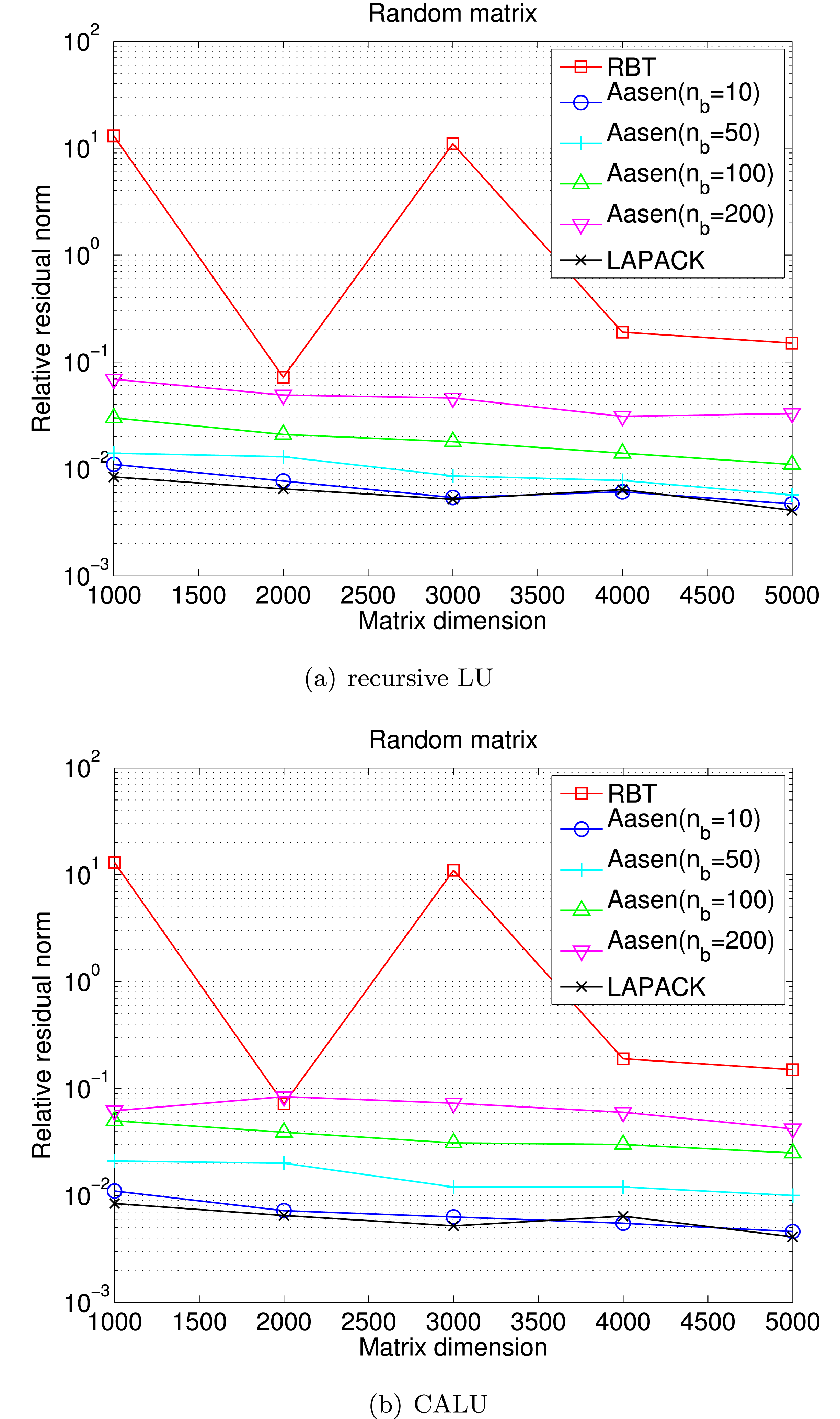
Parallel performance on random matrix with  $n_{b}=250$ on up to eight
 $6$-core
 $2.8$ MHz AMD Opteron processors.
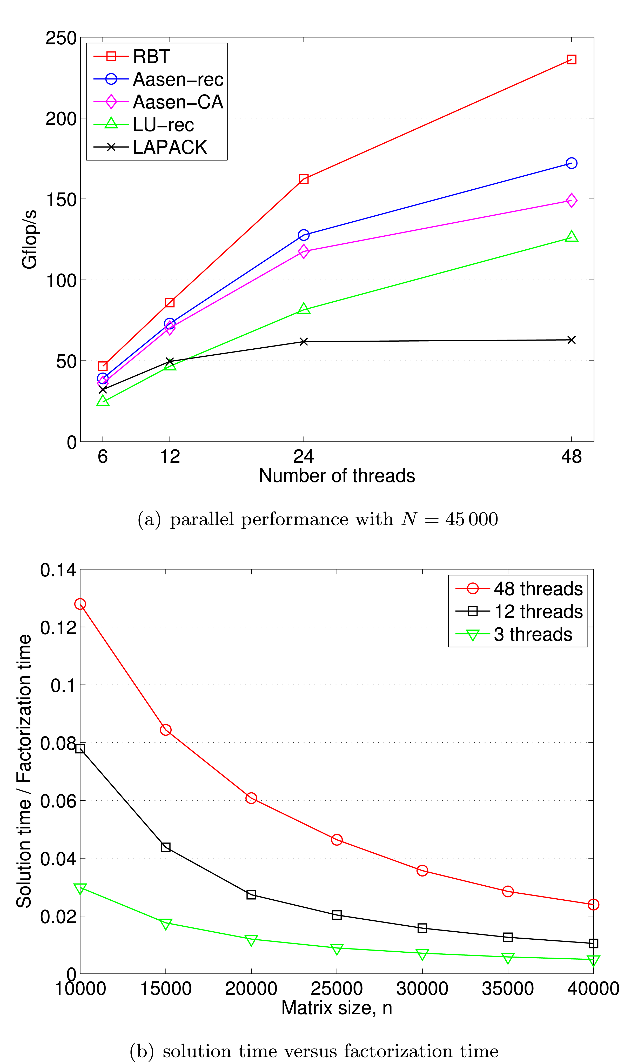
We implemented this blocked Aasen’s algorithm on multicore architectures, and analysed its parallel performance (Ballard et al. Reference Ballard, Becker, Demmel, Dongarra, Druinsky, Peled, Schwartz, Toledo and Yamazaki2013). Our implementation follows the framework of PLASMA and uses a dynamic scheduler called QUARK. To efficiently utilize a large number of cores in parallel, all the existing factorization routines in PLASMA update the trailing submatrix in a right-looking fashion. Hence, our implementation was not only the first parallel implementation of the blocked Aasen’s algorithm, but it was also the first implementation of a left-looking algorithm in PLASMA. In order to fully exploit the limited parallelism in this left-looking algorithm, we studied several performance enhancing techniques (e.g. parallel reduction to update the panel, recursive LU and CALU for panel factorization, and parallel symmetric pivoting). Our performance results on up to 48 AMD Opteron processors demonstrate that a left-looking algorithm can be implemented efficiently on a multicore architecture. In addition, our numerical results show that, in comparison with the widely used stable algorithm (the Bunch–Kaufman algorithm of LAPACK), our implementation loses only one or two digits in the computed residual norms when a recursive LU is used on a panel: see Figure 7.1. Figure 7.2 compares the performance of different algorithms.
7.2 Implementation on multicore CPUs with an accelerator
7.2.1 Bunch–Kaufman algorithm
Our first implementation of the Bunch–Kaufman algorithm is based on a hybrid CPU/GPU programming paradigm where the block column (commonly referred to as a panel) is factorized on the CPUs (e.g. using the threaded MKL), while the trailing submatrix is updated on the GPU. This is often an effective programming paradigm for many of the LAPACK subroutines because the panel factorization is based on Level 1 BLAS or Level 2 BLAS, which can be efficiently implemented on the CPUs, while Level 3 BLAS is used for the submatrix updates, which exhibit high data parallelism and can be efficiently implemented on the GPU. Unfortunately, at each step of the panel factorization, the Bunch–Kaufman algorithm may select the pivot from the trailing submatrix. Hence, although copying the panel from the GPU to the CPU can be overlapped with the update of the rest of the trailing submatrix on the GPU, the look-ahead – a standard optimization technique to overlap the panel factorization on the CPUs with the trailing submatrix update on the GPU – is prohibited. In addition, when the pivot column is on the GPU, this leads to the expensive data transfer between the GPU and the CPU at each step of the factorization. To avoid this expensive data transfer, our second implementation performs the entire factorization on the GPU. Though the CPUs may be more efficient performing the Level 1 BLAS and Level 2 BLAS based panel factorization, this implementation often obtains higher performance by avoiding the expensive data transfer.
When the entire factorization is implemented on the GPU, to select a pivot at each step of the Bunch–Kaufman algorithm, up to two columns of the trailing submatrix must be scanned – the current column and the one with an index corresponding to the row index of the element with the maximum modulus in the first column. This not only leads to the expensive global reduce on the GPU, but also to irregular data accesses since only the lower or upper triangular part of the submatrix is stored. This makes it difficult to obtain high performance on the GPU. In the next two sections, we describe two other algorithms (i.e. communication-avoiding and randomization algorithms) that aim to reduce this bottleneck.
7.2.2 Random butterfly transformation
The application of a depth 1 butterfly matrix is performed using a CUDA kernel where the computed part of the matrix  $A$ is split into blocks. For each of these blocks, the corresponding part of the matrix
 $U$ is stored in the shared memory to improve the memory access performance. Matrix
 $U$ is small enough to fit into the shared memory due to its packed storage.
To compute the LDL $^{\text{T}}$ factorization of the randomized matrix without pivoting, we implemented a block variant of no-pivoting LDL factorization on multicore CPUs with a GPU. In our implementation, the matrix is first copied to the GPU, then the CPU is used to compute the LDL
 $^{\text{T}}$ factorization of the diagonal block. Once the resulting LDL
 $^{\text{T}}$ factors of the diagonal block are copied back to the GPU, the corresponding off-diagonal blocks of the
 $L$-factor are computed by the triangular solve on the GPU. Finally, we update each block column of the trailing submatrix, calling a matrix–matrix multiply on the GPU.
Performance of symmetric factorization on two 8-core Intel Xeon X5680 CPUs with an NVIDIA Kepler K20 GPU (double precision).
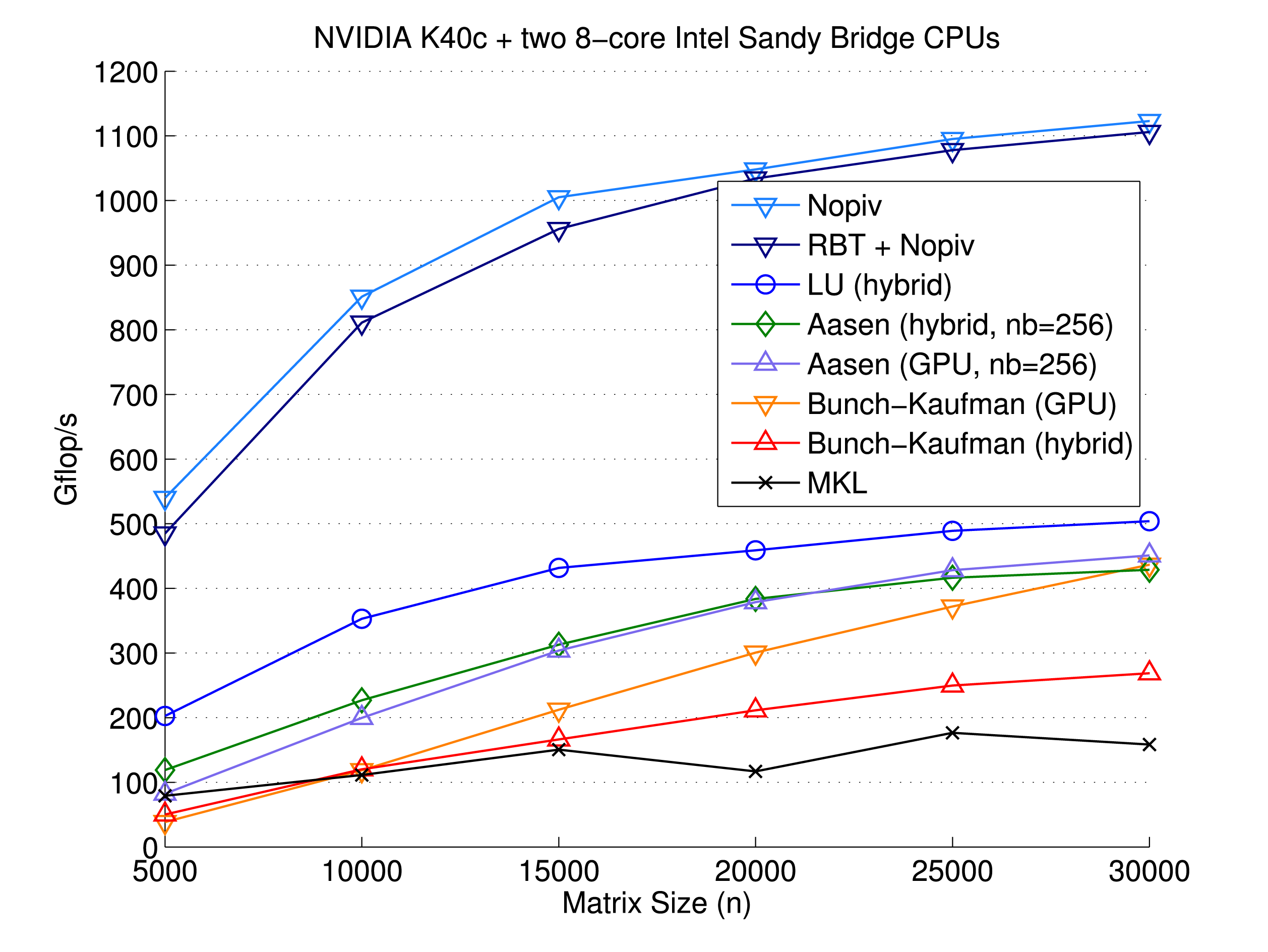
7.2.3 Aasen’s algorithm
Though the GPU has a greater memory bandwidth than the CPU, the memory accesses are still expensive compared to the arithmetic operations. Hence, our implementation is based on the CA Aasen’s algorithm. Though this algorithm performs most of the flops using Level 3 BLAS, most of the operations are on the submatrices of the block size  $n_{b}$. In order to exploit parallelism between the small BLAS calls, we use GPU streams extensively. In addition, for an efficient application of the symmetric pivots after the panel factorization, we apply the pivots in two steps. The first step copies all the columns of the trailing submatrix, which need to be swapped, into an
 $n\times 2n_{b}$ workspace. Here, because of the symmetry, the
 $k$th block column consists of the blocks in the
 $k$th block row and those in the
 $k$th block column. Then, in the second step, we copy the columns of the workspace back to a block column of the submatrix after the column pivoting is applied. The same pivoting strategy is used to exploit the parallelism on multicore CPUs (Ballard et al. Reference Ballard, Becker, Demmel, Dongarra, Druinsky, Peled, Schwartz, Toledo and Yamazaki2013). We tested using the LU factorization with partial pivoting as the panel factorization, either using the threaded MKL on the CPUs or using its native GPU implementation of MAGMA on GPU. Though the Level 1 BLAS and Level 2 BLAS based panel factorization may be more efficient on the CPUs, the second approach avoids the expensive data transfer to copy the panel from the GPU to the CPU. Figure 7.3 compares the performance of different factorization algorithms.
8 Eigenvalue and singular value problems
Solving eigenvalue and singular value problems has many applications across various scientific disciplines; for example, facial recognition (Turk and Pentland Reference Turk and Pentland1991), vibrational analysis of mechanical structures (Cook, Malkus, Plesha and Witt Reference Cook, Malkus, Plesha and Witt2007), seismic reflection tomography (Farra and Madariaga Reference Farra and Madariaga1988), and computing electron energy levels (Singh Reference Singh1994) can all be expressed as eigenvalue problems. Also, the necessity of calculating the singular value decomposition (SVD) emerges from various computational science and engineering areas such as in statistics, where it is directly related to the principal component analysis method (Hotelling Reference Hotelling1933, Reference Hotelling1935), in signal processing and pattern recognition as an essential filtering tool, and in analysis of control systems (Moore Reference Moore1981)). Also, the SVD plays an important role in linear algebra. It has applications in such areas as least-squares problems (Golub and Reinsch Reference Golub, Reinsch, Wilkinson and Reinsch1971), computing the pseudoinverse (Golub and Kahan Reference Golub and Kahan1965), and computing the Jordan canonical form (Golub and Wilkinson Reference Golub and Wilkinson1976). In addition, the SVD is used in solving integral equations (Hanson Reference Hanson1971), digital image processing (Andrews and Patterson Reference Andrews and Patterson1976), information retrieval (Jiang and Berry Reference Jiang, Berry, Ferreira, Rolim, Simon and Teng1998), and optimization (Bartels, Golub and Saunders Reference Bartels, Golub and Saunders1971).
8.1 Background
The eigenvalue problem centres around finding an eigenvector  $x$ and eigenvalue
 ${\it\lambda}$ that satisfy
 $$\begin{eqnarray}Ax={\it\lambda}x,\end{eqnarray}$$
where  $A$ is a symmetric or non-symmetric
 $n\times n$ matrix. When the entire eigenvalue decomposition is computed we have
 $A=X{\rm\Lambda}X^{-1}$, where
 ${\rm\Lambda}$ is a diagonal matrix of eigenvalues and
 $X$ is a matrix of eigenvectors.
The singular value decomposition (SVD) finds orthogonal matrices  $U$ and
 $V$, and a diagonal matrix
 ${\rm\Sigma}$ with non-negative elements, such that
 $$\begin{eqnarray}A=U{\rm\Sigma}V^{T},\end{eqnarray}$$
where  $A$ is an
 $m\times n$ matrix. The diagonal elements of
 ${\rm\Sigma}$ are the singular values of
 $A$, the columns of
 $U$ are its left singular vectors, and the columns of
 $V$ are its right singular vectors.
All these problems are solved by a similar three-phase process.
1 Reduction phase. Orthogonal matrices are applied on the left and right side of
$A$ to reduce it to a condensed form matrix – hence these are called ‘two-sided factorizations’. Note that the use of two-sided transformations guarantees that the reduced matrix has the same eigenvalues or singular values as $A$, and the eigenvectors or singular vectors of $A$ can be easily derived from those of the reduced matrix in phase 3.2 Solution phase. An iterative eigenvalue or singular value solver further reduces the condensed form matrix to compute its eigenvalues or singular values.
3 Eigenvector/singular vector computation phase. If desired, the eigenvectors
$Z$ or singular vectors $\widetilde{U}$ and $\widetilde{V}$ of the condensed form matrix are computed. These are then back-transformed to eigenvectors $X$ or singular vectors $U$ and $V$ of $A$ by multiplying by the orthogonal matrices used in the reduction phase (phase 1). Depending on the algorithm, part or all of phase 3 may be done in conjunction with the solution phase (phase 2).


For the non-symmetric eigenvalue problem, the reduction phase is to upper Hessenberg form,  $H=Q_{1}^{T}AQ_{1}$. For the second phase, QR iteration is used to find the eigenvalues of the reduced Hessenberg matrix
 $H$ by further reducing it to upper triangular Schur form,
 $S=Q_{2}^{T}HQ_{2}$. Since
 $S$ is in upper triangular form, its eigenvalues are on its diagonal and its eigenvectors
 $Z$ can be easily derived. Thus,
 $A$ can be expressed as
 $$\begin{eqnarray}A=Q_{1}HQ_{1}^{T}=Q_{1}Q_{2}SQ_{2}^{T}Q_{1}^{T},\end{eqnarray}$$
which reveals that the eigenvalues of  $A$ are those of
 $S$, and the eigenvectors
 $Z$ of
 $S$ can be back-transformed to eigenvectors of
 $A$ as
 $X=Q_{1}Q_{2}Z$.
When  $A$ is symmetric (or Hermitian in the complex case), the reduction phase is to symmetric tridiagonal,
 $T=Q^{T}AQ$, instead of upper Hessenberg form. Since
 $T$ is tridiagonal, computations with
 $T$ are very efficient. Several eigensolvers are applicable to the symmetric case, such as divide and conquer (D&C), multiple relatively robust representations (MRRR), bisection, and QR iteration. These solvers compute the eigenvalues and eigenvectors of
 $T=Z{\rm\Lambda}Z^{T}$, yielding
 ${\rm\Lambda}$ to be the eigenvalues of
 $A$. Finally, if eigenvectors are desired, the eigenvectors
 $Z$ of
 $T$ are back-transformed to eigenvectors of
 $A$ as
 $X=QZ$.
For the singular value decomposition (SVD), two orthogonal matrices  $Q$ and
 $P$ are applied on the left and right side of
 $A$, respectively, to reduce
 $A$ to bidiagonal form,
 $B=Q^{T}AP$. Divide and conquer or QR iteration is then used as a solver to find both the singular values and the left and right singular vectors of
 $B$ as
 $B=\widetilde{U}{\rm\Sigma}\widetilde{V}^{T}$, yielding the singular values of
 $A$. If desired, singular vectors of
 $B$ are back-transformed to singular vectors of
 $A$ as
 $U=Q\widetilde{U}$ and
 $V^{T}=P^{T}\widetilde{V}^{T}$.
There are many ways to mathematically formulate and numerically solve these problems, but in all cases, designing an efficient computation is challenging because of the nature of the algorithms. In particular, the orthogonal transformations applied to the matrix are two-sided, that is, transformations are applied on both the left and right side of the matrix. This creates data dependencies that prevent the use of standard techniques to increase the computational intensity, such as blocking and look-ahead, which are used extensively in the one-sided LU, QR, and Cholesky factorizations. Thus, the reduction phase can take a large portion of the overall time. Recent research has investigated two-stage algorithms (Lang Reference Lang1999, Bientinesi, Igual, Kressner and Quintana-Ortí Reference Bientinesi, Igual, Kressner and Quintana-Ortí2010, Haidar, Ltaief and Dongarra Reference Haidar, Ltaief and Dongarra2011, Haidar, Ltaief, Luszczek and Dongarra Reference Haidar, Ltaief, Luszczek and Dongarra2012, Ltaief et al. Reference Ltaief, Luszczek, Haidar, Dongarra, Wyrzykowski, Dongarra, Karczewski and Wasniewski2012), where the first stage uses Level 3 BLAS operations to reduce  $A$ to band form, followed by a second stage to reduce it to the final condensed form. Because it is often the most time-consuming phase, it is very important to identify the bottlenecks of the reduction phase, as implemented in the classical approaches (Anderson et al. Reference Anderson, Bai, Bischof, Blackford, Demmel, Dongarra, Ducroz, Greenbaum, Hammarling, McKenney and Sorensen1999).
The initial reduction to condensed form (Hessenberg, tridiagonal, or bidiagonal) and the eigenvector computation are particularly amenable to GPU computation. The eigenvalue solver itself (QR iteration or divide and conquer) has significant control flow and limited parallelism, making it less suited for accelerator computation.
8.2 Singular value decomposition
In this section we will describe, in detail, the three computational phases involved in the singular value decomposition.
8.2.1 The classical reduction to bidiagonal condensed form
Due to its high computational complexity of  $O({\textstyle \frac{8}{3}}n^{3})$ (for square matrices) and interdependent data access patterns, the bidiagonal reduction phase is the most challenging stage to develop and optimize – both algorithmically and from the implementation standpoint. The classical approach from LAPACK (Anderson et al. Reference Anderson, Bai, Bischof, Blackford, Demmel, Dongarra, Ducroz, Greenbaum, Hammarling, McKenney and Sorensen1999) is denoted by ‘one-stage algorithm’, whereby the Householder transformations are grouped and applied in a blocked fashion to directly reduce the dense matrix to bidiagonal form. The one-stage reduction to bidiagonal form suffers from lack of efficiency. To understand it better, one has to focus on the two computational procedures (panel and update) that are repeated until the matrix is reduced. The reduction proceeds by steps of size
 $n_{b}$. Below we give the detailed cost of step
 $i$, as a cost for the panel and a cost for the update.
∙ The panel factorization computes the similarity transformations (Householder reflectors) to introduce zeros to the entries below the subdiagonal within a single block of
$n_{b}$ columns. The factorization of every column is dominated primarily by two matrix–vector products with the trailing matrix. Thus, this computation is critical as the entire trailing submatrix needs to be loaded into memory, and very few floating-point operations are executed on all of the transferred data. As the memory bandwidth becomes more limited and does not scale with the number of cores, the panel factorization step is not expected to scale for large matrices that do not fit in cache. The cost of a panel is $4n_{b}l^{2}+{\rm\Theta}(n)$, where $l$ is the size of the trailing matrix. For simplicity, we omit ${\rm\Theta}(n)$ and round up the cost of the panel by the cost of the matrix–vector product.∙ The trailing submatrix update consists of applying the Householder reflectors, generated during the panel factorization, to the trailing matrix from both the left and right side using compute-bound operations that utilize Level 3 BLAS, which have a high data re-use ratio allowing for highly tuned implementations. In addition, Level 3 BLAS lend themselves to parallelization due to their inherent data locality properties, which can be exploited to achieve high performance rates for large amounts of operations, with most of it completely independent and thus perfectly suited to multicore processors. Unfortunately, each panel factorization must be synchronized with the corresponding update of the trailing submatrix, which prevents asynchronous execution and overlap of memory-bound and compute-bound steps that could potentially alleviate the effects of the former. The computational cost of this procedure is
where$$\begin{eqnarray}A_{i+n_{b}:n,i+n_{b}:n}\leftarrow A_{i+n_{b}:n,i+n_{b}:n}-V\times Y^{T}-X\times U^{T},\end{eqnarray}$$$V$ and $Y$ are the Householder reflectors computed during the panel phase, $X$ and $Y$ are two rectangular matrices needed for the update, and also computed during the panel phase. This update phase can be performed by two matrix–matrix products using the GEMM routine, and its cost is $2\times 2n_{b}k^{2}$, where $k$ is the size of the trailing matrix at step $i$.





The percentage of the time spent in each phase of the SVD solver using the classical one-stage approach to compute the bidiagonal form.
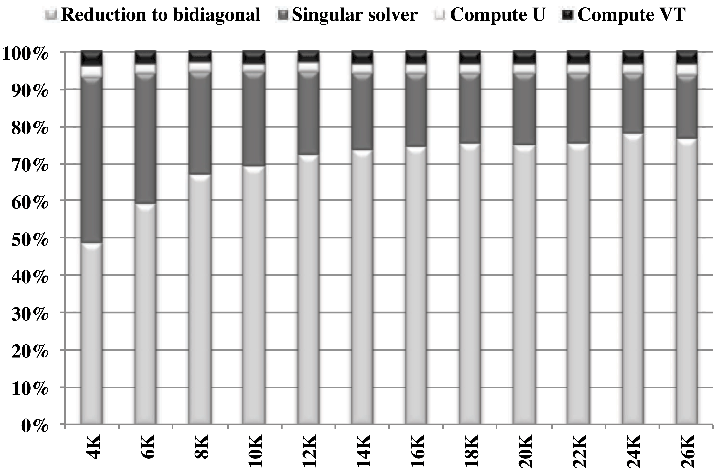
For all steps ( $n/n_{b}$), the trailing matrix size varies from
 $n$ to
 $n_{b}$ by steps of size
 $n_{b}$, where
 $l$ varies from
 $n$ to
 $n_{b}$ and
 $k$ varies from
 $(n-n_{b})$ to
 $2n_{b}$. Thus the total cost for the
 $n/n_{b}$ steps is
 $$\begin{eqnarray}{\approx}4n_{b}\mathop{\sum }_{n_{b}}^{n/n_{b}}l^{2}+4n_{b}\mathop{\sum }_{2n_{b}}^{\frac{n-n_{b}}{n_{b}}}k^{2}\approx \frac{4}{3}n_{\mathtt{GEMV}}^{3}+\frac{4}{3}n_{\text{Level 3}}^{3}\approx \frac{8}{3}n^{3}.\end{eqnarray}$$
Following the equations above, we derive the maximum performance  $P_{\max }$ that can be reached by any of these reduction algorithms. In particular, for large matrix sizes
 $n$,
 $$\begin{eqnarray}P_{\max }=\frac{\text{number of operations}}{\text{minimum time }t_{\min }},\end{eqnarray}$$
and thus  $P_{\max }$ is expressed as
 $$\begin{eqnarray}\frac{\frac{8}{3}n^{3}}{\frac{4}{3}n^{3}\ast \frac{1}{P_{\mathtt{GEMV}}}+\frac{4}{3}n^{3}\ast \frac{1}{P_{\text{Level 3}}}}=\frac{2\ast P_{\text{Level 3}}\ast P_{\mathtt{GEMV}}}{P_{\text{Level 3}}+P_{\mathtt{GEMV}}}\approx 2P_{\mathtt{GEMV}}\end{eqnarray}$$
when  $P_{\text{Level 3}}\gg P_{\mathtt{GEMV}}$. Thus, equation (8.2) proves the well-known low-performance behaviour of the classical bidiagonal reduction algorithm, and for that it is considered the most time-consuming phase. Figure 8.1 shows the percentage of the total time for each of the four components of the SVD solver using the standard one-stage reduction approach when all the singular vectors are computed. The figure makes it clear that the reduction to the bidiagonal form requires more than 70% of the total time for the case when all the singular vectors are computed. In addition, when only singular values are needed, the reduction requires about 90% of the total computing time. Because of the expense of the reduction step, renewed research has focused on improving this step, resulting in a novel technique based on a ‘two-stage’ algorithm (Lang Reference Lang1999, Bientinesi et al. Reference Bientinesi, Igual, Kressner and Quintana-Ortí2010, Haidar et al. Reference Haidar, Ltaief and Dongarra2011, Haidar et al. Reference Haidar, Ltaief, Luszczek and Dongarra2012, Ltaief et al. Reference Ltaief, Luszczek, Haidar, Dongarra, Wyrzykowski, Dongarra, Karczewski and Wasniewski2012, Haidar, Kurzak and Luszczek Reference Haidar, Kurzak and Luszczek2013a), where a first stage uses Level 3 BLAS operations to reduce
 $A_{s}$ to band form, and a second stage further reduces the matrix to the proper bidiagonal form. We developed our singular value solver based on the ‘two-stage’ techniques, which allow us to exploit more parallelism and use recent hardware more efficiently.
Two-stage technique for the reduction phase.
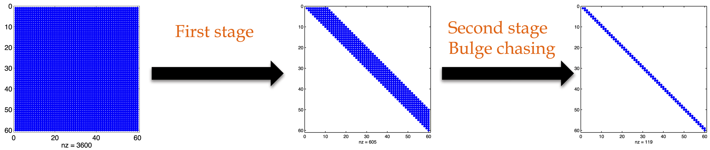
8.2.2 Two-stage reduction
The two-stage reduction is designed to overcome the limitations of the one-stage approach, which relies heavily on memory-bound operations. It also increases the use of compute-intensive operations that benefit from the increase in CPU core count. Many algorithms have been studied extensively in the context of the symmetric eigenvalue problems (Bischof, Lang and Sun Reference Bischof, Lang and Sun2000, Bischof and Van Loan Reference Bischof and Van Loan1987), and, more recently, tile algorithms have achieved good performance (Luszczek, Ltaief and Dongarra Reference Luszczek, Ltaief and Dongarra2011, Haidar et al. Reference Haidar, Ltaief and Dongarra2011). The idea behind them is to split the original one-stage approach into a compute-intensive phase (first stage) and a memory-bound phase (second or bulge chasing stage) as represented in Figure 8.2. The first stage reduces the original general dense matrix to a band form (either upper or lower), and the second stage reduces the band form to the canonical bidiagonal form (again, either upper or lower). The two-stage approach is used in our implementation, and exhibits some similarities to what has been developed for the symmetric eigenvalue problem (Haidar et al. Reference Haidar, Ltaief and Dongarra2011). To put our work into a proper perspective, we start by briefly describing the first stage (reduction from full dense to band), and then we explain in more detail the reduction from band to bidiagonal form. We will also talk about the scheduling techniques on which our implementation relies.
First stage: compute-intensive and efficient kernels.
The first stage applies a sequence of blocked Householder transformations to reduce the general dense matrix to either an upper or a lower band matrix. This stage uses compute-intensive matrix-multiply kernels that eliminate the memory-bound matrix–vector product from the one-stage panel factorization. It also illustrates a beneficial data access pattern through the use of compute-intensive operations based on Level 3 BLAS for large portions of the code (Bischof et al. Reference Bischof, Lang and Sun2000, Dongarra, Sorensen and Hammarling Reference Dongarra, Sorensen and Hammarling1989, Gansterer, Kvasnicka and Ueberhuber Reference Gansterer, Kvasnicka and Ueberhuber1999, Haidar et al. Reference Haidar, Tomov, Dongarra, Solcà and T.2014). Moreover, this stage is made highly parallel because of the tile algorithm formulation (Agullo, Hadri, Ltaief and Dongarra Reference Agullo, Hadri, Ltaief and Dongarra2009b), which brings the parallelism to the fore. Conceptually and physically, the matrix is split into  $nt\times nt$ tiles (
 $nt=n/nb$,
 $nb$ is the size of the tile and the resulting matrix bandwidth). The data within a tile is stored contiguously in memory. The algorithm then proceeds as a collection of interdependent tasks that operate on the tile data layout. Figure 8.3 highlights the execution breakdown during the second step of the first stage of the reduction. A QR factorization is computed for the tile
 $A_{2,2}$ (the solid grey tile). After this QR is finished, a set of independent tasks is released and they can all be executed in parallel. All tiles
 $A_{2,\bullet }$ (the black tiles of Figure 8.3(a)) can be updated by applying the Householder transformations that are generated by the QR factorization of
 $A_{2,2}$. Also, all the tiles
 $A_{\bullet ,2}$ (the grey diamond pattern tiles of Figure 8.3(a)) can also be independently annihilated one after another with the R factor of
 $A_{2,2}$. After each tile
 $A_{i,2}$ is annihilated (e.g. the black checkerboard pattern tile of Figure 8.3(a)), a set of parallel tasks may be launched to update all the tiles of the block row
 $i$ (the stripe pattern tiles of Figure 8.3(a)). Moreover, when
 $A_{2,3}$ is updated, then an LQ factorization is performed for this tile (the solid grey tile of Figure 8.3(b)). Similarly to the QR process, after LQ, all the tiles in the third column of tiles,
 $A_{3:nt,3}$ (the grey diamond pattern tiles of Figure 8.3(b)), can now be independently updated by the Householder vectors from the LQ factorization, provided that they have been updated with the transformation from the QR factorization. Similarly, all the tiles
 $A_{2,4:nt}$ (the black checkerboard pattern tiles of Figure 8.3(b)) can also be annihilated. Likewise, each annihilation of
 $A_{1,i}$ (the black checkerboard pattern tile of Figure 8.3(b)) enables a set of tasks to update the block column
 $i$ (the stripe pattern tiles of Figure 8.3(b)). We note that this requires implementations of new computational kernels to be able to operate on the new data structures. The details of the implementation of this stage are provided elsewhere (Haidar et al. Reference Haidar, Ltaief and Dongarra2011, Luszczek et al. Reference Luszczek, Ltaief and Dongarra2011). This process of interleaving the QR and the LQ factorizations at each step repeats until the end, and, as a result, we obtain a band matrix with a bandwidth of size
 $nb$. As we mentioned above, the tile formulation of the algorithm resulted in the creation of a large number of parallel tasks. These tasks are organized into a directed acyclic graph (DAG) (Buttari et al. Reference Buttari, Dongarra, Kurzak, Langou, Luszczek, Tomov, Kågström, Elmroth, Dongarra and Wasniewski2006, Chan, Quintana-Orti, Quintana-Orti and van de Geijn Reference Chan, Quintana-Orti, Quintana-Orti and van de Geijn2007), with the nodes representing the computational tasks and the edges – the data dependencies between them. Thus, restructuring the linear algebra algorithms as a sequence of tasks that operate on tiles of data removes the fork–join bottleneck that befits the LAPACK-style implementations. It also avoids idle time for individual cores, while, at the same time, increasing the data locality for each core. Moreover, in order to increase the efficiency of our algorithm, we improved our dynamic scheduler by developing two main features that played an important role in targeting high-performance execution rates. Two auxiliary options were added to the scheduler that allow us to label some of the tasks PRIORITY and LOCALITY. For example, when the QR factorization of
 $A_{1,1}$ and a sequence of QR updates ensues, it is better to increase the priority of all the tasks that modify the tile
 $A_{1,2}$, in such a way that the LQ process of
 $A_{1,2}$ starts as soon as possible. As a result, this technique will increase the number of parallel tasks and will aid the interleaving of the tasks from both the QR and the LQ update sequences. As described below, this has a big impact on data locality. The second task label that we developed is the LOCALITY flag. It is used for the update of any tile of
 $A_{2:n,2:n}$. It makes it possible for
 $A_{2,2}$ to be updated by the QR’s Householder process and by the LQ Householder process. Hence, our scheduler has an opportunity to let the same core update
 $A_{2,2}$ by the two transformations, one after the other. This will result in the tile data being loaded from the main memory only once.
Kernel execution of the BRD algorithm during the first stage.
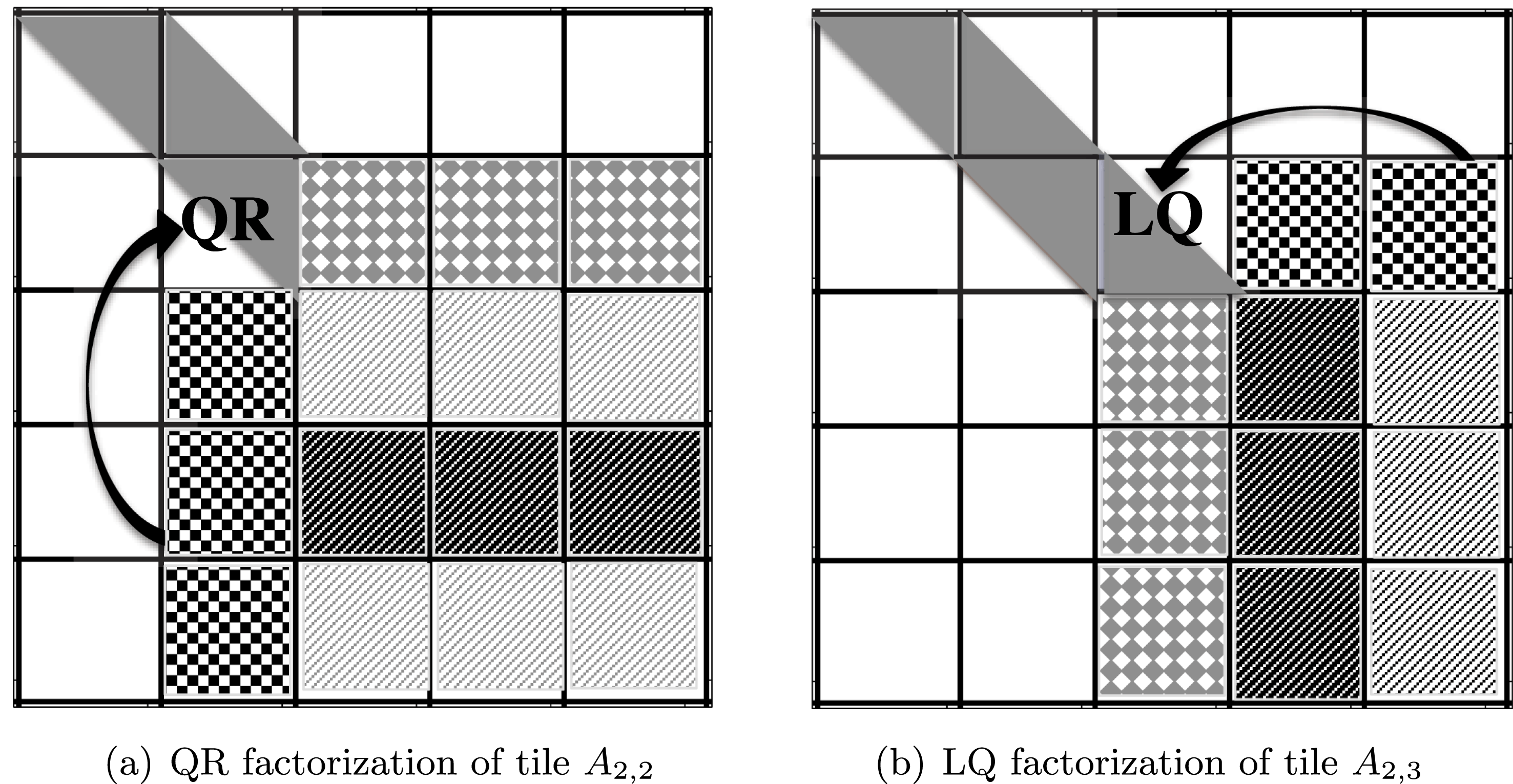
Second stage: cache-friendly computational kernels.
The band form is further reduced to the final condensed form using the bulge chasing technique. This procedure annihilates the extra off-diagonal elements by chasing the created fill-in elements down to the bottom right side of the matrix using successive orthogonal transformations at each sweep. This stage involves memory-bound operations and requires the band matrix to be accessed from multiple disjoint locations. In other words, there is an accumulation of substantial latency overhead each time different portions of the matrix are loaded into cache memory, which is not compensated for by the low execution rate of the actual computations (the so-called surface-to-volume effect). To overcome these critical limitations, we developed a bulge chasing algorithm, very similar to the novel bulge chasing techniques for symmetric eigenvalue problems (reduction from band to bidiagonal) developed in Haidar et al. (Reference Haidar, Ltaief and Dongarra2011), but we differ from it in using a column-wise elimination instead of an element-wise elimination. In addition, we also differ by developing our kernels to deal with general matrices instead of symmetric matrices. When the singular vectors need to be computed, the most problematic aspect of the standard procedure is the element-wise elimination (Haidar et al. Reference Haidar, Ltaief and Dongarra2011). Such an implementation is very suitable when only singular value is required, but is limited when singular vectors are required. In particular, it generates element-wise Householder reflectors, and thus the update of the singular vectors by these reflectors becomes the bottleneck as it is based on Level 1 BLAS operations. Our modification adds a small amount of extra work, but it allows the use of the Level 3 BLAS kernels to compute the transformations or to apply them in the form of the orthogonal matrix  $U_{2}$ and
 $V_{2}$ – the result of computation in this phase. Moreover, we designed our algorithm to extensively use cache-friendly kernels combined with fine-grained, memory-aware tasks in an out-of-order scheduling technique which considerably enhances data locality.
Kernel execution of the BRD algorithm during the second stage.
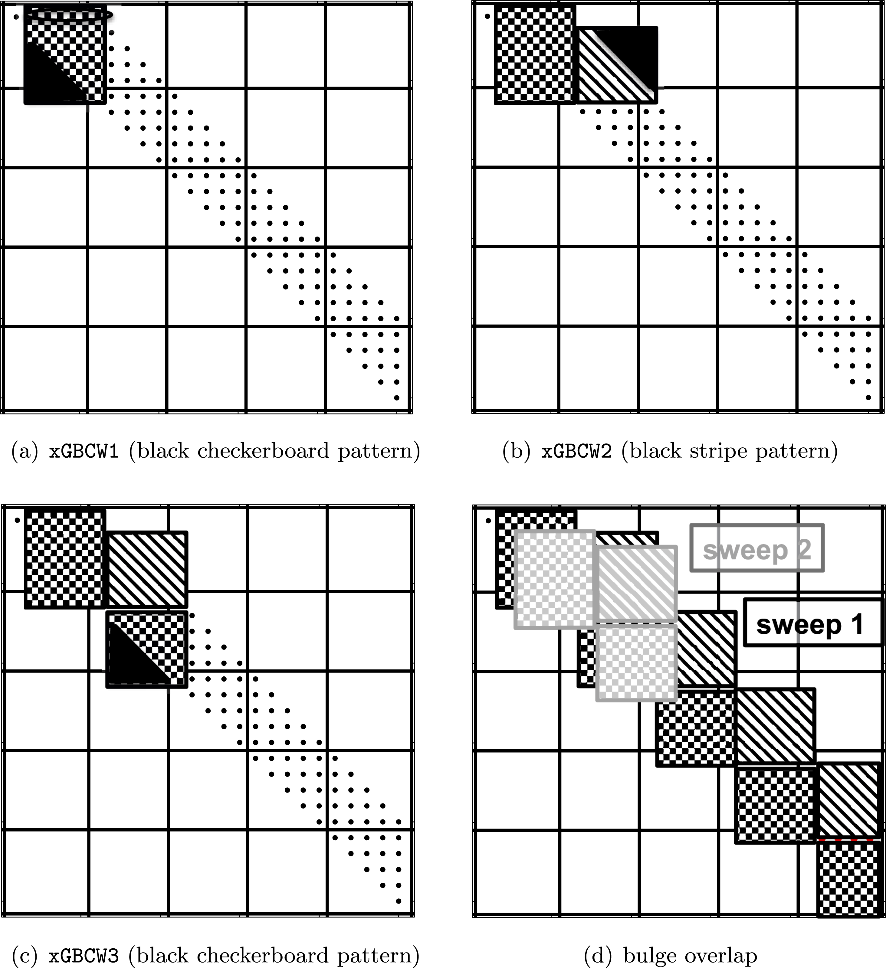
The bulge chasing algorithm consists of a succession of three new kernels designed to increase cache re-use. The idea is to load a block of data in the actual cache memory and to apply all the possible computation to it before unloading it. The first kernel, called xGBCW1 and illustrated in Figure 8.4(a), manipulates the black checkerboard pattern block of data. It triggers the beginning of each sweep by annihilating the extra non-zero entries within a single row, then applies the computed elementary Householder reflector from the right within this block. Hence, it subsequently generates triangular bulges as shown in Figure 8.4(a) (the black block). Note that this triangular bulge must be annihilated eventually in order to avoid the excessive growth of the fill-in structure. A classical implementation will eliminate the whole triangular bulge. However, for an appropriate study of the bulge chasing procedure, let us remark that the elimination of the row  $i+1$ (the sweep
 $i+1$), at the next step, creates a triangular bulge which will overlap this one-by-one column shift to the right and one row to the bottom, as shown in Figure 8.4(d), where the reader can see that the lower triangular portion of the grey checkerboard pattern block (the bulge created in sweep
 $i+1$) overlaps with the lower triangular portion of the black checkerboard pattern block (corresponding to the bulges created by the previous sweep
 $i$). As a result, we can reduce the computational cost, and instead of eliminating the whole triangular bulge created for sweep
 $i$, we only eliminate the non-overlapped region of it – its first column. The remaining columns can be delayed to the upcoming annihilation sweeps. In this way, we can avoid the growth of the bulges and reduce the extra cost accrued when the whole bulge is eliminated. Moreover, we designed a cache-friendly kernel that takes advantage of the fact that the created bulge (the black checkerboard pattern block) remains in the cache and therefore it directly eliminates its first column and applies the corresponding left update to the remaining column of the black checkerboard pattern block. The second kernel, xGBCW2, loads the next block and it applies the necessary left updates derived from the previous kernel. This will eventually generate triangular bulges as shown in Figure 8.4(b). Hence, this kernel will also annihilate the first row of the created bulge and update its black stripe pattern block from the right. Finally, the third kernel, xGBCW3, loads the next block (the third black checkerboard pattern block of Figure 8.4(c)) and it continues applying, from the right, the transformations of the previous kernel 2. Like kernel 1, it also creates a bulge which is removed, and the black checkerboard pattern block is updated correspondingly from the left, similar to the process undertaken by kernel 1. Accordingly, the annihilation of each sweep can be described as a single call to kernel 1 followed by repetitive calls to a cycle of kernel 2 and kernel 3.
The implementation of this stage is done by using either a dynamic or a static runtime environment, whose detailed implementation we developed and discussed in Haidar et al. (Reference Haidar, Kurzak and Luszczek2013a, Reference Haidar, Tomov, Dongarra, Solcà and T.2014). This stage is, in our opinion, one of the main challenges for algorithms as it is difficult to track the data dependencies. The annihilation of the subsequent sweeps will generate computational tasks, which will partially overlap within the data used by the tasks of the previous sweeps (see Figure 8.4(d)) – the main challenge of dependency tracking. We have used our data translation layer (DTL) and functional dependencies (Luszczek et al. Reference Luszczek, Ltaief and Dongarra2011, Haidar et al. Reference Haidar, Ltaief and Dongarra2011) to handle the dependencies and to provide crucial information to the runtime to achieve the correct scheduling. As mentioned above, the amount of data involved with each task is of size  $nb\times nb$, but is handled efficiently because our kernels increase cache re-use. We also developed our scheduling technique to minimize the memory traffic and increase the efficiency of our algorithm in such a way that the subsequent tasks that involve the same region of data will be executed by the same thread. As an example, the first task
 $T_{1}^{(2)}$ of the annihilation of sweep 2, which operates on the grey stripe pattern block of Figure 8.4(d), overlaps the region of the data that has been used by the first task
 $T_{1}^{(1)}$ of the sweep 1 (black checkerboard pattern block). However, it is obvious to execute task
 $T_{1}^{(2)}$ by the same thread that executed
 $T_{1}^{(1)}$. To ensure maximum re-use, we force the scheduler to distribute the tasks according to their data location. The main goal of our data-based scheduling is to define fine-grained local tasks that increase cache re-use and minimize communication. For small matrix sizes, we prefer the use of a subsequent set of threads (the number of threads that fit the matrix into its fast memory) while leaving the other threads working on different portions of the code rather than using all the available resources. The implementation of this phase has been well optimized. It has been observed that it takes between 5% and 10% of the global time of the reduction from dense to bidiagonal.
8.2.3 The bidiagonal singular solver
A bidiagonal singular solver computes the spectral decomposition of a bidiagonal matrix  $B$ such that
 $$\begin{eqnarray}B=\widetilde{U}{\rm\Sigma}\widetilde{V}^{H}\quad \text{with }\widetilde{U}\widetilde{U}^{H}=I\text{ and }\widetilde{V}\widetilde{V}^{H}=I,\end{eqnarray}$$
where  $\widetilde{U}$ and
 $\widetilde{V}^{H}$ are the singular vectors and
 ${\rm\Sigma}$ the singular values of
 $B$. There are two main implementations of the singular solver, one based on the QR algorithm (Golub and Kahan Reference Golub and Kahan1965), and one based on the divide and conquer algorithm (Jessup and Sorensen Reference Jessup and Sorensen1989, Gu and Eisenstat Reference Gu and Eisenstat1995).
8.2.4 The singular vector computation
The classical one-stage approach reduces the dense matrix  $A$ to bidiagonal
 $B$ and computes its singular values and vectors. The singular values of
 $A$ are the same as the
 ${\rm\Sigma}$ computed for the bidiagonal matrix
 $B$. The singular vectors of
 $A$ (
 $U$ and
 $V^{H}$) are computed from the left and right singular vectors of
 $B$ by applying the same orthogonal matrices
 $Q$ and
 $P^{H}$ that were used in the reduction to condensed form, respectively, that is,
 $$\begin{eqnarray}\displaystyle \begin{array}{@{}rclcl@{}}U\ & =\ & Q\widetilde{U}\ & =\ & (I-V_{1}T_{1}V_{1}^{H})\widetilde{U},\\ \text{and}\quad V^{H}\ & =\ & \widetilde{V}^{H}P_{1}^{H}\ & =\ & \widetilde{V}^{H}(I-W_{1}Tr_{1}^{H}W_{1}^{H}),\end{array} & & \displaystyle\end{eqnarray}$$
where ( $V_{1},T_{1}$ and
 $W_{1},Tr_{1}$) represent the left and right Householder reflectors generated during the reduction to the bidiagonal form, respectively. From this representation, either
 $Q$ and
 $P^{H}$ can be formed explicitly using DORGBR; or we can multiply by
 $Q$
 $P^{H}$ in an implicit fashion using DORMBR, which is less expensive. In either case, applying
 $Q$ and
 $P^{H}$ becomes a series of DGEMM operations. Algorithm 7 describes the back transformation of the one-stage reduction to the left singular vectors. The same will be applied to the right vectors. The cost of this phase is equal to
 $2n^{3}$ for each singular vector. Since all of its computation is based on Level 3 BLAS, the performance upper bound of this phase is considered to be on a par with the performance of the Level 3 BLAS, which is usually a large fraction of the peak of the machine.

In the case of the two-stage approach, the first stage reduces the original general dense matrix  $A$ to a general band matrix by applying a two-sided transformation to
 $A$ such that
 $Q_{1}^{H}AP_{1}=A_{\text{band}}$. Similarly, the second stage – bulge chasing – reduces the band matrix
 $A_{\text{band}}$ to the bidiagonal form by applying the transformation from both the left and right side to
 $A_{\text{band}}$ such that
 $Q_{2}^{H}A_{\text{band}}P_{2}=B$. Let us now denote the SVD of
 $A$ by
 $A=U{\rm\Sigma}V^{H}$, where
 $U$ and
 $V^{H}$ are, respectively, the left and right singular vectors of
 $A$, and the diagonal entries of
 ${\rm\Sigma}$ hold the singular values. These singular vectors must be multiplied by both of
 $Q_{\ast }$ and
 $P_{\ast }$, according to
 $$\begin{eqnarray}\begin{array}{@{}rclcl@{}}U\ & =\ & Q_{1}Q_{2}\widetilde{U}\ & =\ & (I-V_{1}T_{1}V_{1}^{H})(I-V_{2}T_{2}V_{2}^{H})\widetilde{U},\\ \text{and}\quad V^{H}\ & =\ & \widetilde{V}^{H}P_{2}^{H}P_{1}^{H}\ & =\ & \widetilde{V}^{T}(I-W_{2}Tr_{2}^{H}W_{2}^{H})(I-W_{1}Tr_{1}^{H}W_{1}^{H}),\end{array}\end{eqnarray}$$
where ( $V_{1},T_{1}$ and
 $W_{1},Tr_{1}$) and (
 $V_{2},T_{2}$ and
 $W_{2},Tr_{2}$) represent the left and right Householder reflectors generated during the first and second stages of the reduction to the bidiagonal form. It is clear that the two-stage approach introduces a non-trivial amount of extra computation – the application of
 $Q_{2}$ and
 $P_{2}^{H}$ – for the case when the singular vectors are needed. Thus, one of the crucial procedures of the two-stage algorithm, when optimizing for performance, is the update of the singular vectors by the Householder transformations that were generated during the two stages of the reduction to the bidiagonal form. Obviously, the implementation of this scheme is not as straightforward as simply parallelizing a loop. In particular, because of complications of the bulge chasing mechanism, the order of generated task dependencies is quite intricate. Due to the geometric shape of non-zero entries during the second stage of the reduction from
 $A_{\text{band}}$ to bidiagonal, called bulge chasing, the application of
 $Q_{2}$ and
 $P_{2}$ has to follow the order mentioned in Figure 8.5, where each application consists of the diamond shape of the
 $V$ applied to
 $U$. Figure 8.5 shows the Householder reflectors for both stages. More details of the optimized technique to apply
 $Q_{2}$ and
 $P_{2}$ can be found in Haidar, Luszczek and Dongarra (Reference Haidar, Luszczek and Dongarra2014b). The algorithm for the update of
 $U$ using
 $Q_{2}$ is described in Algorithm 7, and the cost of this step can be summarized by a
 $$\begin{eqnarray}2\biggl(1+\frac{i_{b}}{n_{b}}\biggr)n^{3}\end{eqnarray}$$
operation using the Level 3 BLAS. Similarly, the cost of applying  $P_{2}^{H}$ can be computed in the same manner.
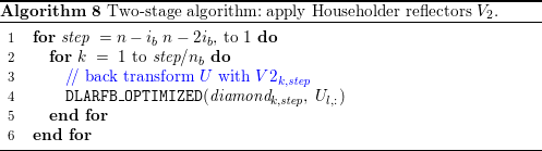
(a) Tiling of  $V_{1}$. (b) Blocking used to apply
 $V_{2}$.
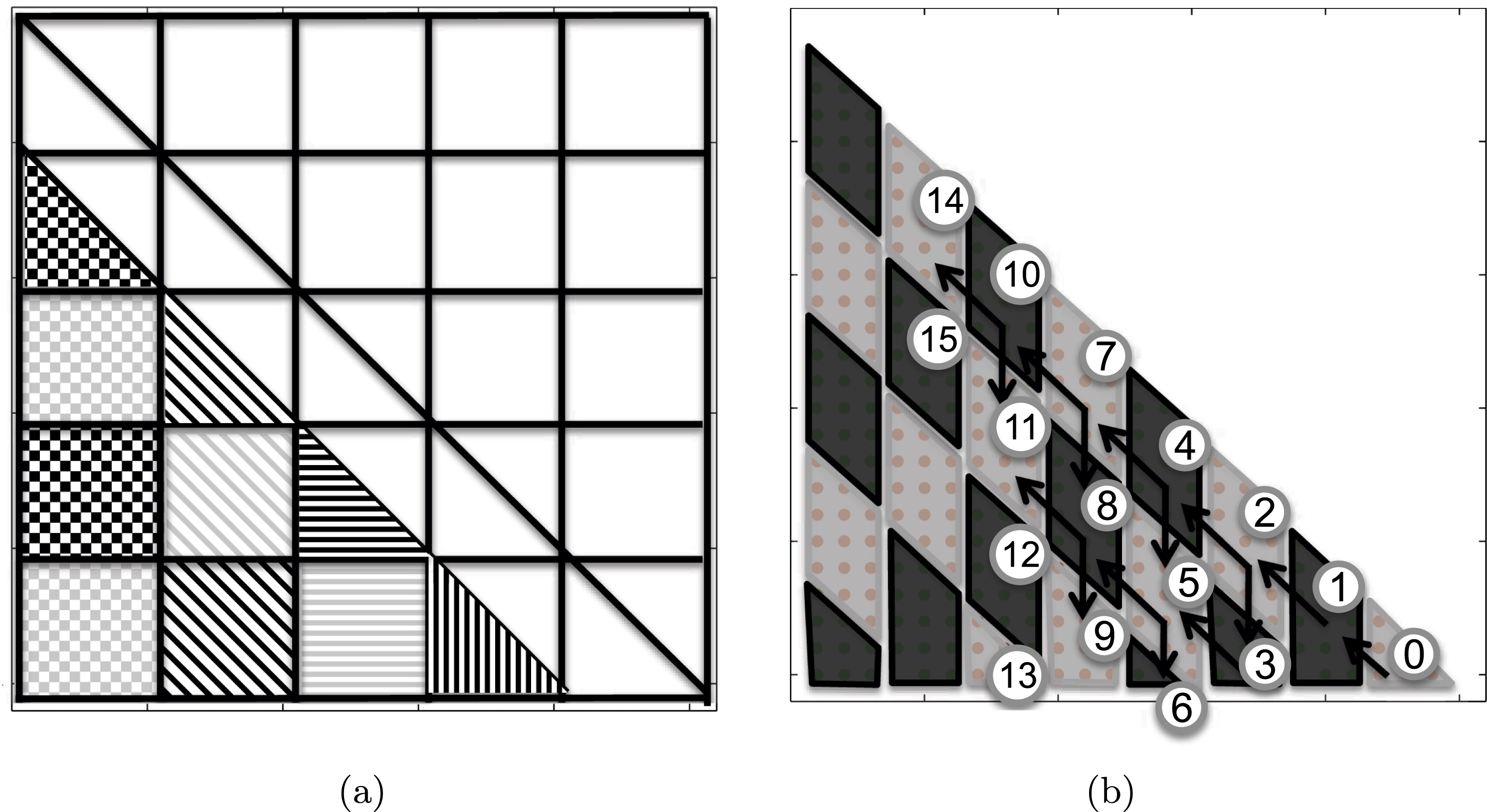

The application of  $Q_{1}$ can be done easily and efficiently using our tile algorithm (Haidar et al. Reference Haidar, Luszczek and Dongarra2014b) and is described in Algorithm 9. The parallelism in this step comes from two sources: first, the singular vector matrix is viewed as a set of independent tiles to be updated; second, the parallelism can also be extracted by applying
 $Q_{1}$ as a set of independent Householder reflectors, row-wise, meaning that the only constraint to follow is their column-wise order (e.g., once the Householder reflector of block
 $(i,j)$ has been applied, that of block
 $(i,j-1)$ can be applied). As a result, the design of the tile algorithm generates a large number of independent tasks that can be applied in an asynchronous manner using either a static or a dynamic scheduler. The
 $V_{1}$ are stored in a tile fashion, as shown in Figure 8.5, to increase data locality. The total cost of this step is approximately
 $2n^{3}$. Consequently, the total cost of updating the singular vectors when using the two-stage techniques is
 $$\begin{eqnarray}2\biggl(1+\frac{i_{b}}{n_{b}}\biggr)n^{3}+2n^{3}\end{eqnarray}$$
for the left singular vectors and the same for the right singular vectors. Compared to the one-stage approach, we can observe that the two-stage technique has an extra cost of the order of
 $$\begin{eqnarray}2\biggl(1+\frac{i_{b}}{n_{b}}\biggr)n^{3}\end{eqnarray}$$
operations for the left singular vector and the same for the right singular vector.
Hence, when only the singular values are computed, our new two-stage implementation is expected to be largely advantageous when compared to the classic algorithm (e.g., it can reach about  $7\times$ speedup). However, when computing the left and right singular vectors, our two-stage approach has an extra cost of
 $$\begin{eqnarray}2\times 2\biggl(1+\frac{i_{b}}{n_{b}}\biggr)n^{3}\end{eqnarray}$$
operations from the back-transformation of the second stage. This will clearly affect the roughly  $8\times$ observed speedup for the reduction to the bidiagonal form. However, since the extra cost is computed by the Level 3 BLAS operations, one can expect that we can still get speedup over the classical approach – particularly for accelerated architectures. Our experiments described in the next section show that we can reach still reach up to
 $2\times$ speedup on a multicore architecture when both the left and right singular vectors are computed. Also, one can expect that if a percentage of the singular vectors is needed, the extra cost is dramatically decreased, and a speedup of about
 $5\times$ was observed.
8.2.5 Experimental results
This section presents the performance comparisons of our tile algorithm for two-stage SVD against state-of-the-art numerical linear algebra libraries.
Experimental environment.
We performed our experiments on two shared memory systems. These systems are representative server-grade machines and workstations commonly used for computationally intensive workloads. The first system, named system A, is composed of four sockets of AMD Opteron 6180 SE CPUs, 12 cores each (48 cores total), running at 2.5 GHz with 128 GB of main memory; the total number of cores is evenly spread between two physical motherboards. The Level 2 cache size per core is 512 KB. The theoretical peak for this architecture in double precision is 480 Gflops (10.1 Gflops per core). Our second system, named system B, is composed of two sockets of Intel Xeon E5-2670 (Sandy Bridge) CPUs, eight cores each (16 cores total), each running at 2.6 GHz with 52 GB of main memory. Each socket has 24 MB of shared L3 cache, and each core has a private 256 KB L2 and 64 KB L1 cache. The theoretical peak for this architecture in double precision is 333 Gflops (20.8 Gflops per core).
There are a number of software packages that include a singular value decomposition solver. For comparison, we used the latest MKL (Math Kernel Library)Footnote 4 version 13.1, which is a commercial library from Intel that is highly optimized for Intel processors and competes with alternatives on AMD processors. MKL includes a comprehensive set of mathematical routines implemented to run well on most x86 multicore processors. In particular, MKL includes LAPACK-equivalentFootnote 5 routines to compute the bidiagonal reduction DGEBRD, and routines to find the singular value decomposition such as DGESDD (the divide and conquer (D&C) algorithm) and DGESVD (the implicit zero-shift QR algorithm).
Performance results.
The following experiments illustrate the superior efficiency and the scalability of our proposed SVD solver with respect to the state-of-the-art optimized vendor numerical linear algebra libraries. Each graph below presents comparison curves that we will describe. We performed an extensive study with a large number of experiments on two different machines (one with a large number of cores, system A, and another with small number of cores, system B) in order to give the reader as much information as possible. We computed the SVD decomposition, where we either compute only the singular values, or both singular values and vectors, with two different algorithms (DGESVD, DGESDD), varying the size of the matrices from  $2000$ to
 $26\,000$ using our two systems described above. Since many applications only need a portion of the singular vectors, we also present results using DGESDD (the divide and conquer SVD solver) to compute 20% of the singular vectors. In addition, in order to make our experiments self-contained, we report the result of the improvements that our two-stage implementation brought to the reduction to bidiagonal form, compared against the one-stage approach from the state-of-the-art numerical linear algebra libraries.
The speedup obtained by our implementation of DGESDD versus its counterpart from the Intel MKL library on 48 AMD cores of system A.
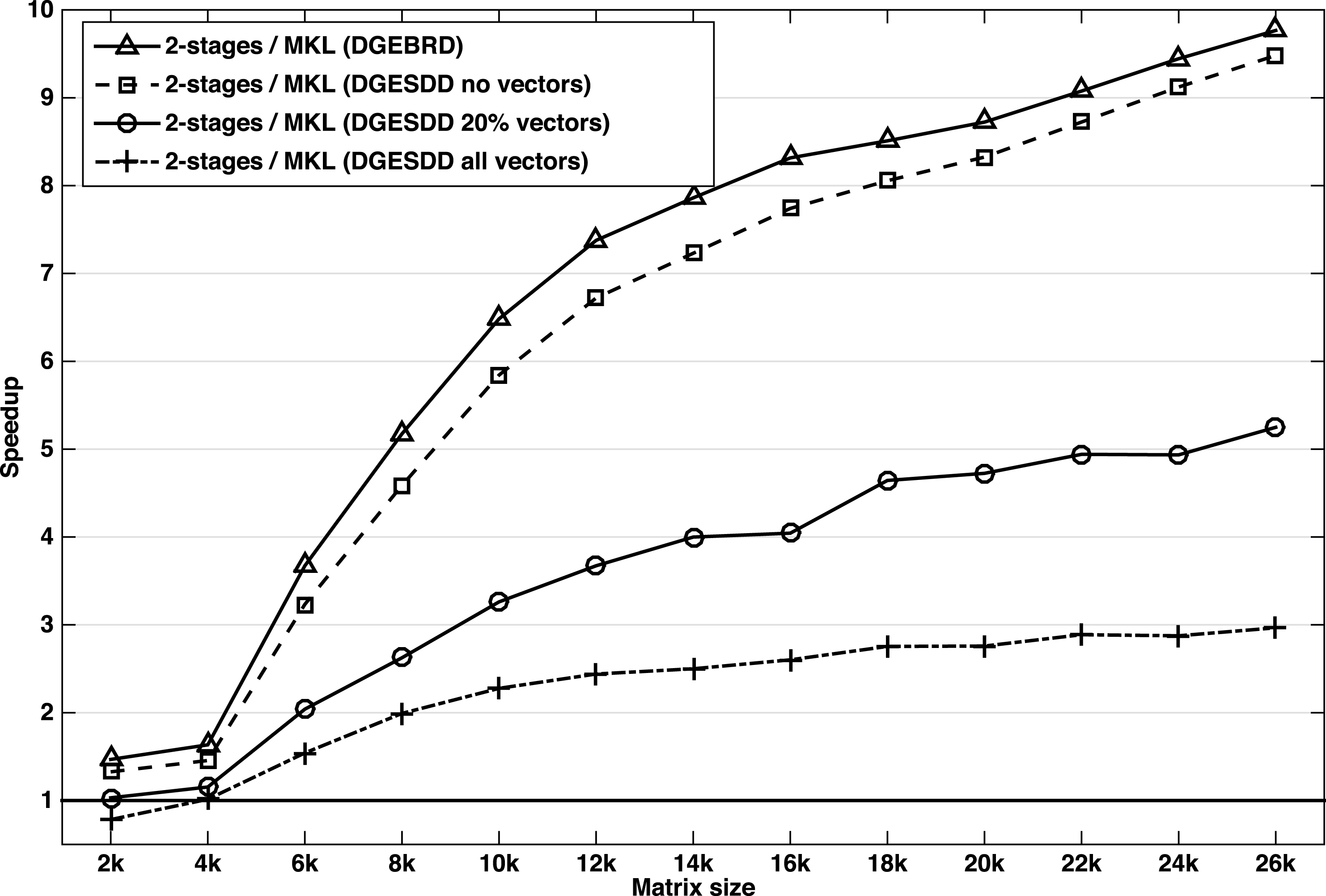
The speedup obtained by our implementation of DGESDD versus its counterpart from the Intel MKL library on 16 Sandy Bridge cores of system B.
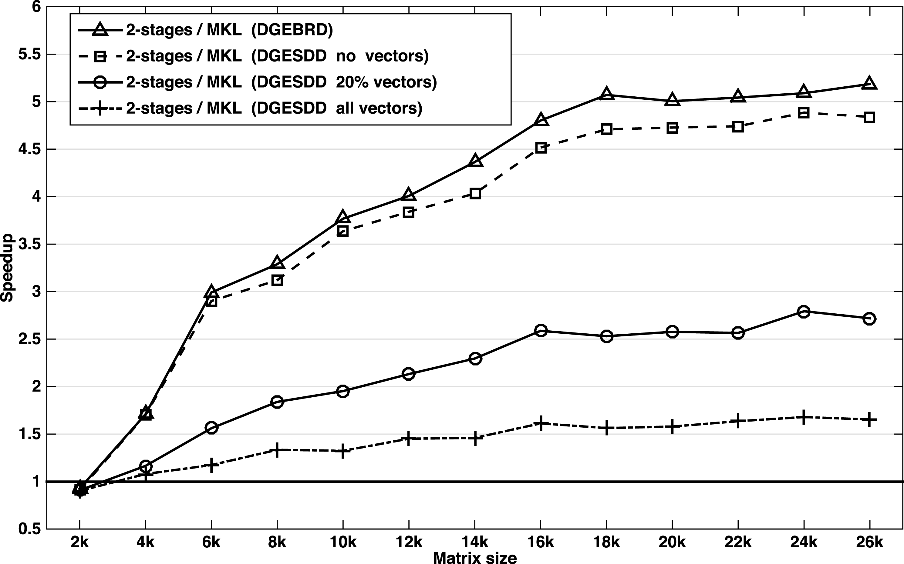
In particular, Figures 8.6 and 8.7 show speedups and efficiencies for computing the SVD using the divide and conquer technique. For each speedup curve (representing a routine), we depict the ratio of the runtime between the routine from Intel’s MKL library and its counterpart from our implementation within the same computing environment. These results show four types of behaviour.
Let us first comment on the reduction to bidiagonal form (DGEBRD: triangles) and on the SVD decomposition when only the singular values are computed (DGESDD NO Vectors: squares). The speedups shown are remarkable, our implementation asymptotically achieves more than  $8\times$ speedup on the 48 cores of system A and more than
 $4\times$ speedup on the 16 cores of system B. This was not unexpected, and the results obtained here confirm the importance of the considerations discussed in our study when designing high-performance libraries. The performance gain is due to the tile algorithm that we developed and to its efficient implementation of the first stage (reduction to band), which is the compute-intensive stage, and from the design of both the second stage (bulge chasing) and the orthogonal transformation update, which maps both the algorithm and the data to the hardware using cache-friendly kernels and scheduling based on increasing data locality. Our new algorithm scales as the matrix sizes increase and asymptotically achieves a perfect speedup, despite the side effects of running on a NUMA system.
In contrast to the standard approach where the reduction to bidiagonal dominates the overall time (as described above in Figure 8.1), the two-stage reduction to bidiagonal consists of less than 20% of the overall time. Thus, when only singular values or a small portion of the vectors are needed, our approach is particularly favourable. One of the most fruitful advantages of our two-stage SVD algorithm is the attractive speedup shown when a portion of the singular vectors is computed. The performance obtained by DGESDD, when 20% of the singular vectors are required, shows more than a  $4\times$ increase when using the 48 cores of system A (circles in Figure 8.6), and can get more than
 $2\times$ speedup when using the 16 cores of system B (circles in Figure 8.7). The underlying results are straightforward. The computing portion of the singular vectors significantly minimizes the overhead of the extra cost (applying
 $Q_{2}$ and
 $P_{2}$) introduced by the two-stage approach, and therefore the speedup observed here is relatively high.
Moreover, we also evaluated the performance and speedup of our algorithm when all the singular vectors are computed (diamonds in Figures 8.6 and 8.7). We can observe that our algorithm performs consistently better than the state-of-the-art optimized MKL routine DGESDD, with the exception of small matrices. Our implementation is around  $3\times$ faster when using a large number of cores (48 cores of system A) and is around
 $1.5\times$ faster on a smaller number of cores (16 cores of system B).
Our fourth observation is related to the scalability of our implementation. To explain it briefly, we performed experiments with only 12 cores of system A, and compared it with the results from the full 48 cores. Our solver accomplished very good scalability: the execution time on 48 cores is about  $3.5\times$ faster than the one obtained on 12 cores. It also appears from the speedup illustrated in our figures that the scalability increases with respect to the number of cores, and for that reason we believe that this implementation is suitable for large distributed and shared memory machines.
The speedup obtained by our implementation of DGESVD versus its counterpart from the Intel MKL library on 48 AMD cores of system A.
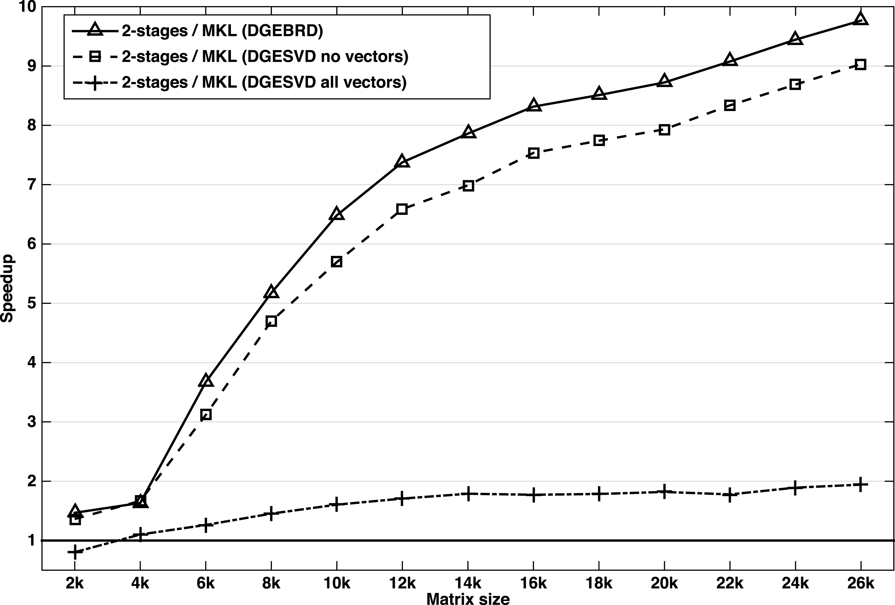
The speedup obtained by our implementation of DGESVD versus its counterpart from the Intel MKL library on 16 Sandy Bridge cores of system B.
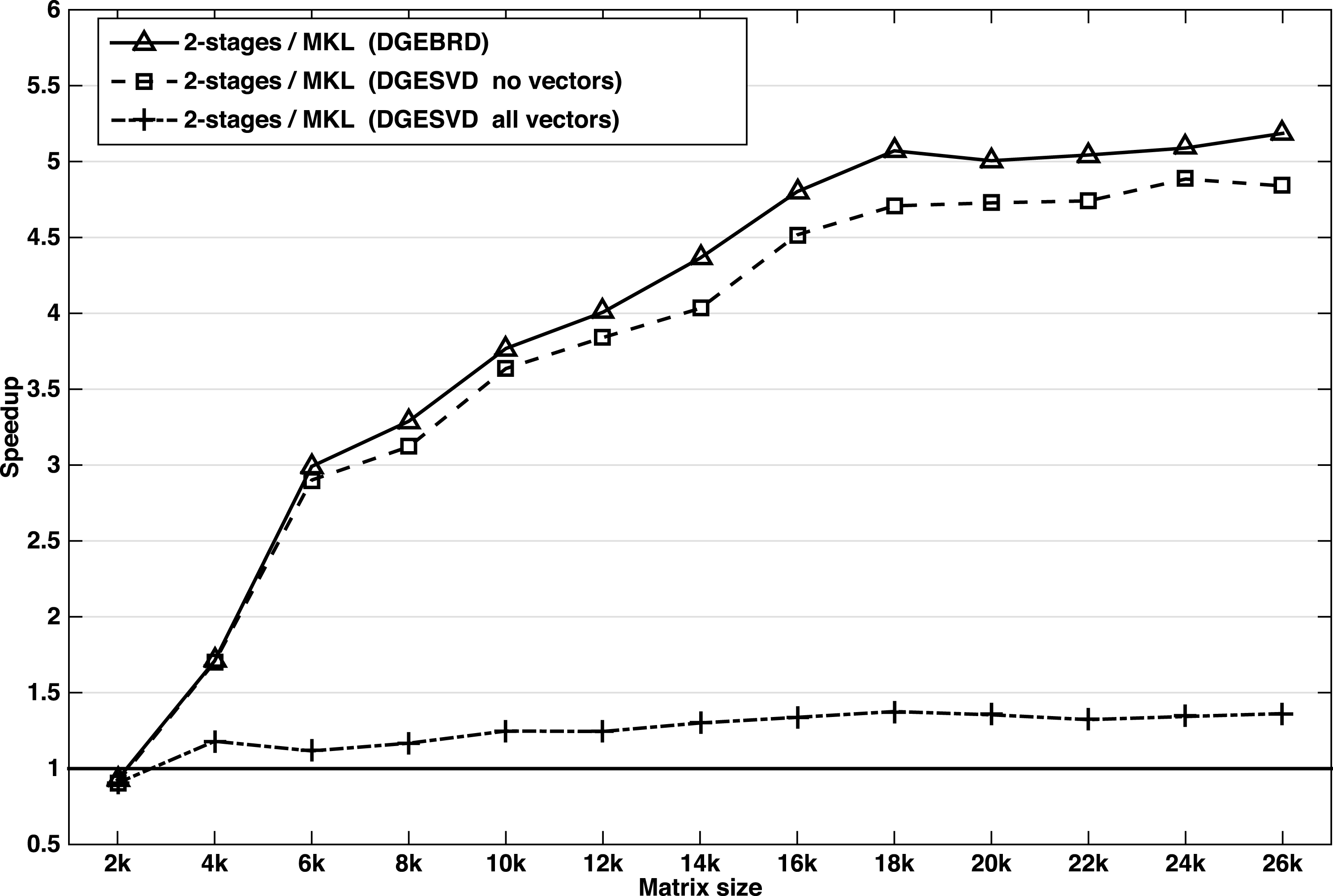
Since we prefer to cover all the available SVD solvers and not be limited by the divide and conquer technique, we also performed the same set of experiments using the implicit zero-shift QR algorithm (DGESVD) as another solver variant. The speedup results obtained on both of our machines, system A and system B, are presented in Figures 8.8 and 8.9, respectively. Here we note that we could not compute a set of the singular vectors because the routine which computes the SVD decomposition of the bidiagonal matrix (DBDSQR) does not provide this option, and requires the transformation matrices  $Q$ and
 $P^{H}$ to be provided explicitly as input. However, experiments with either all the singular vectors or none of the singular vectors were reported. The speedup of the DGEBRD routine has been reported in Figures 8.8 and 8.9, for the sake of completeness.
The performance shown in Figures 8.8 and 8.9 is very close to that of the divide and conquer solver. The performance drops slightly compared to Figures 8.6 and 8.7, because the DBDSQR solver used here requires the matrix  $Q$ and
 $P$ to be computed explicitly as input, and so it updates the singular vectors
 $L_{s}$ and
 $R_{s}$ internally. Thus it does not benefit from all the optimizations we implemented. However, the explicit generation of the matrices
 $Q$ and
 $P$ take advantage of all the techniques described in this section. As a consequence, the speedup curve trend in Figures 8.8 and 8.9 slightly decreases compared to that of Figures 8.6 and 8.7. Therefore, reaching a twofold speedup (Figure 8.8) is worth the effort.
Finally, we demonstrate that our algorithm is very efficient and can achieve more than a twofold speedup over the well-known state-of-the-art optimized libraries. It is especially suitable when only the singular values – or when a portion of the singular vectors – are needed. Results show a  $4\times$ to
 $10\times$ speedup. We believe that this achievement makes our algorithm a very good candidate for current and next generation computing hardware.
8.3 Symmetric eigenvalue problem
In a similar fashion to our discussion of singular value decomposition above, we will now describe the three phases of the symmetric eigenvalue solver.
8.3.1 The classical reduction to tridiagonal condensed form
The classical approach (LAPACK algorithms) to reducing a matrix to tridiagonal form is to use a one-stage algorithm (Golub and Van Loan Reference Golub and Van Loan1996). Similar to the one-sided factorizations (Cholesky, LU, QR), the two-sided factorizations are split into a panel factorization and a trailing matrix update. Unlike the one-sided factorizations, however, the panel factorization requires computing the Level 2 BLAS symmetric matrix–vector product with the entire trailing matrix. This requires loading the entire trailing matrix into memory, which incurs a significant amount of memory-bound operations. It creates data dependencies and produces artificial synchronization points between the panel factorization and the trailing submatrix update steps. This prevents the use of standard techniques to increase the computational intensity (e.g. look-ahead), which are used extensively in the one-sided LU, QR, and Cholesky factorizations. Let us compute the cost of the algorithm. The reduction proceeds by steps of size  $n_{b}$, where each step consists of the cost of the panel and the cost of the update.
∙ The panel is of size
$n_{b}$ columns. The factorization of every column is dominated primarily by one symmetric matrix–vector product with the trailing matrix. Thus the cost of a panel is where$$\begin{eqnarray}2n_{b}l^{2}+{\rm\Theta}(n),\end{eqnarray}$$$l$ is the size of the trailing matrix. For simplicity, we omit ${\rm\Theta}(n)$ and round up the cost of the panel by the cost of the matrix–vector product.∙ The update of the trailing matrix consists of applying the Householder reflectors generated during the panel factorization to the trailing matrix from both the left and right side according to
where$$\begin{eqnarray}A_{i+n_{b}:n,i+n_{b}:n}\leftarrow A_{i+n_{b}:n,i+n_{b}:n}-V\times W^{T}-W\times V^{T},\end{eqnarray}$$$V$ and $W$ were computed during the panel phase. This Level 3 BLAS operation is computed by the SYR2K routine and its cost is $2n_{b}k^{2}$, where $k=n-in_{b}$ is the size of the trailing matrix at step $i$.


For all steps ( $n/n_{b}$), the trailing matrix size varies from
 $n$ to
 $n_{b}$, by steps of size
 $n_{b}$, where
 $l$ varies from
 $n$ to
 $n_{b}$ and
 $k$ varies from
 $(n-n_{b})$ to
 $2n_{b}$. Thus, the total cost for the
 $n/n_{b}$ steps is
 $$\begin{eqnarray}\text{flops}\approx 2n_{b}\mathop{\sum }_{n_{b}}^{n/n_{b}}l^{2}+2n_{b}\mathop{\sum }_{2n_{b}}^{\frac{n-n_{b}}{n_{b}}}k^{2}\approx \frac{2}{3}n_{\mathtt{SYMV}}^{3}+\frac{2}{3}n_{\mathtt{SYR2K}}^{3}\approx \frac{4}{3}n^{3}.\end{eqnarray}$$
According to the equations above, we derive the maximum performance  $P_{\max }$ that can be reached by such an algorithm. In particular, for large matrix sizes
 $n$,
 $P_{\max }$ is expressed as
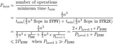 $$\begin{eqnarray}\displaystyle P_{\max } & = & \displaystyle \frac{\text{number of operations}}{\text{minimum time }t_{\min }}\nonumber\\ \displaystyle & = & \displaystyle \frac{\frac{4}{3}n^{3}}{t_{\min }({\textstyle \frac{2}{3}}n^{3}\text{ flops in }\mathtt{SYMV})+t_{\min }(\frac{2}{3}n^{3}\text{ flops in }\mathtt{SYR2K})}\nonumber\\ \displaystyle & = & \displaystyle \frac{\frac{4}{3}n^{3}}{\frac{2}{3}n^{3}\ast \frac{1}{P_{\mathtt{SYMV}}}+\frac{2}{3}n^{3}\ast \frac{1}{P_{\text{Level 3}}}}=\frac{2\ast P_{\text{Level 3}}\ast P_{\mathtt{SYMV}}}{P_{\text{Level 3}}+P_{\mathtt{SYMV}}}\nonumber\\ \displaystyle & \leq & \displaystyle 2P_{\mathtt{SYMV}}\quad \text{when }P_{\text{Level 3}}\gg P_{\mathtt{SYMV}}.\end{eqnarray}$$
Thus, from equation (8.7) we can understand the well-known low-performance behaviour of the classical tridiagonal reduction algorithm. In practice, it is the most time-consuming phase (about 70% of the time when all eigenvectors are requested, and about 90% of the time when only eigenvalues are needed). Figure 8.10 depicts the percentage of the time spent in each phase of the eigensolver using the classical one-stage approach to compute the tridiagonal form and eigenvectors.
The percentage of the time spent in each phase of the eigensolver using the classical one-stage approach for the tridiagonal reduction.
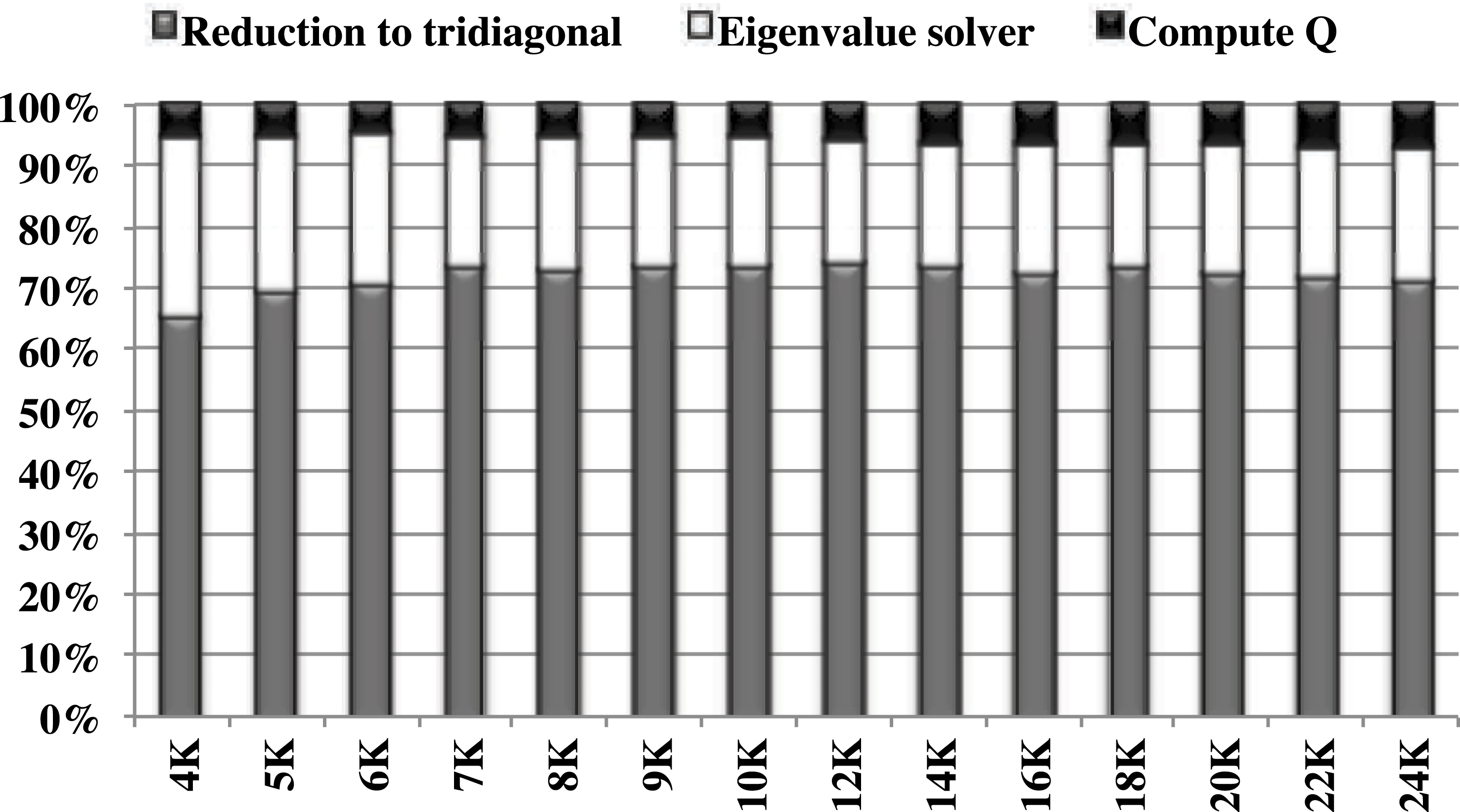
8.3.2 Two-stage reduction
Similarly to the singular value decomposition, we can take advantage of the two-stage approach for the reduction to tridiagonal form. The two-stage reduction is designed to increase the utilization of compute-intensive operations. Many algorithms have been investigated using this two-stage approach. The idea is to split the original one-stage approach into a compute-intensive phase (first stage) and a memory-bound phase (second or ‘bulge chasing’ stage). In this section we will cover the description for the symmetric case. The first stage reduces the original symmetric dense matrix to a symmetric band form, while the second stage reduces from band to tridiagonal form, as depicted in Figure 8.11. The same algorithm used for reducing the general matrix  $A$ to band form in the singular value decomposition case (Section 8.2.2) can be adapted to the symmetric case, where the symmetric matrix
 $A$ is reduced to tridiagonal form.
Two-stage technique for the reduction phase.
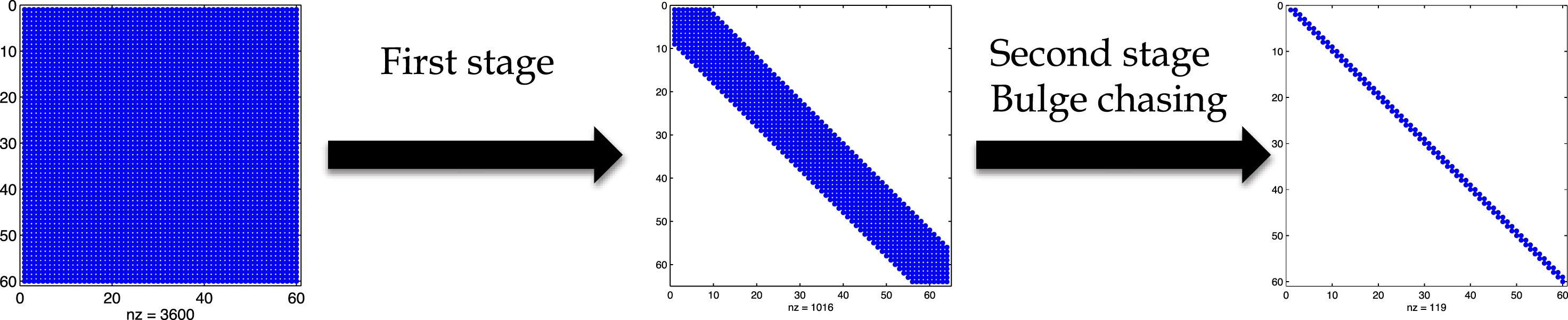
First stage: compute-intensive and efficient kernels.
The first stage applies a sequence of block Householder transformations to reduce a symmetric dense matrix to a symmetric band matrix  $A\longrightarrow A_{\text{band}}$. This stage uses compute-intensive matrix-multiply kernels, eliminating the memory-bound matrix–vector product in the one-stage panel factorization, and has been shown to have a good data access pattern and large portion of Level 3 BLAS operations (Dongarra et al. Reference Dongarra, Sorensen and Hammarling1989, Gansterer et al. Reference Gansterer, Kvasnicka and Ueberhuber1999, Haidar et al. Reference Haidar, Tomov, Dongarra, Solcà and T.2014). Given a dense
 $n\times n$ symmetric matrix
 $A$, the matrix is divided into
 $nt=n/b$ tiles of size
 $nb$.
The algorithm proceeds tile by tile, performing a QR decomposition for each tile to generate the Householder reflectors  $V$ (i.e. the orthogonal transformations) required to zero out elements below the bandwidth
 $nb$. Then the generated block Householder reflectors are applied from the left and right to the trailing symmetric matrix. The algorithm is described in Algorithm 10.
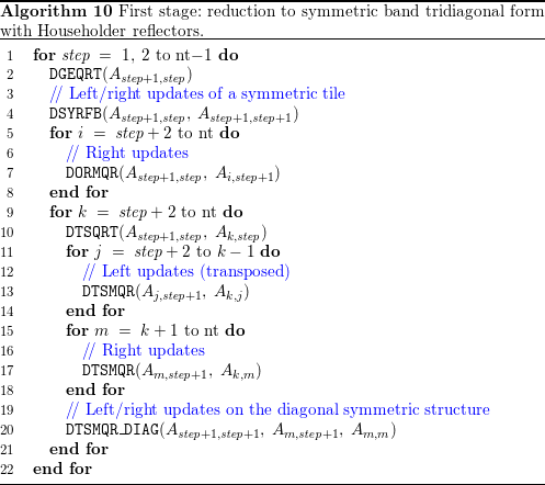
Since the factorization consists of a QR factorization performed on a tile of size  $nb\times nb$ shifted by
 $nb$ rows below the diagonal, this will remove both the synchronization and the data dependency constraints seen using the classical one-stage technique. In contrast to the classical approach, the panel factorization by itself does not require any operation on the data of the trailing matrix, making it an independent task. Moreover, we can factorize the next panel once we have finished its update, without waiting for the total trailing matrix update. As a result, this kind of technique removes the bottlenecks of the classical approach: there are no Level 2 BLAS operations concerning the trailing matrix and there is also no need to wait to finish the update of the whole trailing matrix in order to start the next panel. Note that this technique is well suited for accelerators. Recent work can be found in Haidar et al. (Reference Haidar, Solcà, Gates, Tomov, Schulthess, Dongarra, Kunkel, Ludwig and Meuer2013b, Reference Haidar, Tomov, Dongarra, Solcà and T.2014) and Solcà et al. (Reference Solcà, Kozhevnikov, Haidar, Tomov, Dongarra and Schulthess2015).
Second stage: cache-friendly computational kernels.
The band matrix  $A_{\text{band}}$ is further reduced to the tridiagonal form
 $T$ using the bulge chasing technique, similar to the one described in Section 8.2.2, but using kernels designed for a symmetric case. This procedure annihilates the extra off-diagonal elements by chasing the created fill-in elements down to the bottom right side of the matrix using successive orthogonal similarity transformations. Each annihilation of the
 $n_{b}$ non-zero element below the off-diagonal of the band matrix is called a sweep, as described in Figure 8.12. This stage involves memory-bound operations and requires the band matrix to be accessed from multiple disjoint locations. In other words, there is an accumulation of substantial latency overhead each time different portions of the matrix are loaded into cache memory, which is not compensated for by the low execution rate of the actual computations (the so-called surface-to-volume effect). To overcome these critical limitations, we used a bulge chasing algorithm to use cache-friendly kernels, combined with fine-grained memory-aware tasks, in an out-of-order scheduling technique, which considerably enhances data locality. We refer the reader to Haidar et al. (Reference Haidar, Ltaief and Dongarra2011, Reference Haidar, Tomov, Dongarra, Solcà and T.2014) for a detailed description of the technique.
Two-stage technique for the reduction phase.

8.3.3 The tridiagonal eigensolver
The tridiagonal eigensolver is used to compute eigenpairs of the tridiagonal matrix:
 $$\begin{eqnarray}T=Z{\rm\Lambda}Z^{T},\end{eqnarray}$$
where  $Z$ is the matrix of orthogonal eigenvectors of
 $T$, and
 ${\rm\Lambda}$ is the diagonal matrix encoding the eigenvalues. Four algorithms are available: QR iterations, bisection and inverse iteration (BI), divide and conquer (D&C), and multiple relatively robust representations (MRRR). The first two, QR and BI, are presented in Demmel (Reference Demmel1997), but a performance comparison made by Demmel, Marques, Parlett and Vomel (Reference Demmel, Marques, Parlett and Vomel2008b) compared LAPACK algorithms and concluded that D&C and MRRR are the fastest available solvers. However, while D&C requires a larger extra workspace, MRRR is less accurate. Accuracy is a fundamental parameter, because the tridiagonal eigensolver is known to be the part of the overall symmetric eigensolver where accuracy can be lost. D&C is more robust than MRRR, which can fail to provide an accurate solution in some cases. In theory, MRRR is a
 ${\rm\Theta}(n^{2})$ algorithm, whereas D&C is between
 ${\rm\Theta}(n^{2})$ and
 ${\rm\Theta}(n^{3})$, depending on the matrix properties. In many real-life applications, D&C is often less than cubic, while MRRR seems to be slower than expected due to the number of floating divisions and the cost of the iterative process. The main asset of MRRR is that a subset computation is possible, reducing the complexity to
 ${\rm\Theta}(nk)$ for computing
 $k$ eigenpairs. Such an option was not included within the classical D&C implementations, or it only reduced the cost of the updating phase of the last step of the algorithm.
8.3.4 The eigenvector computation
After the reduction to condensed form, the eigensolver finds the eigenvalues  ${\rm\Lambda}$ and eigenvectors
 $Z$ of
 $T$. The eigenvalues are the same as for the original matrix
 $A$. To find the eigenvectors of the original matrix
 $A$, the eigenvectors
 $Z$ of
 $T$ need to be back-transformed by applying the same orthogonal matrices (e.g.
 $Q$ for the one-stage approach or
 $Q_{1}$ and
 $Q_{2}$ for the two-stage approach) that were used in the reduction to condensed form. For this purpose, the block Householder transformations
 $Q_{i}=I-V_{i}T_{i}V_{i}^{T}$ are used. For the one-stage approach, there is only one
 $Q$ that has been used in the reduction phase, and its multiplication by
 $Z$ can be formed explicitly using DORGTR; or we can multiply by
 $Q$ in an implicit fashion using DLARFB following the procedure described in Algorithm 7. In either case, applying
 $Q$ becomes a series of DGEMM operations. Since all of its computation is based on Level 3 BLAS, the performance upper bound of this phase is considered to be on a par with the performance of the Level 3 BLAS, which is usually a large fraction of the machine’s peak, and – for this phase – is considered to be a small percentage of the global time of the eigensolver. Figure 8.10 illustrates the percentage of time occupied by the one-stage algorithm’s three phases, and we can see that this phase consumes less than 10% of the total time.
Speedup of our new two-stage implementation over the classic one-stage approach when both eigenvalues and eigenvectors are computed on 28 Intel E5-2697 cores.
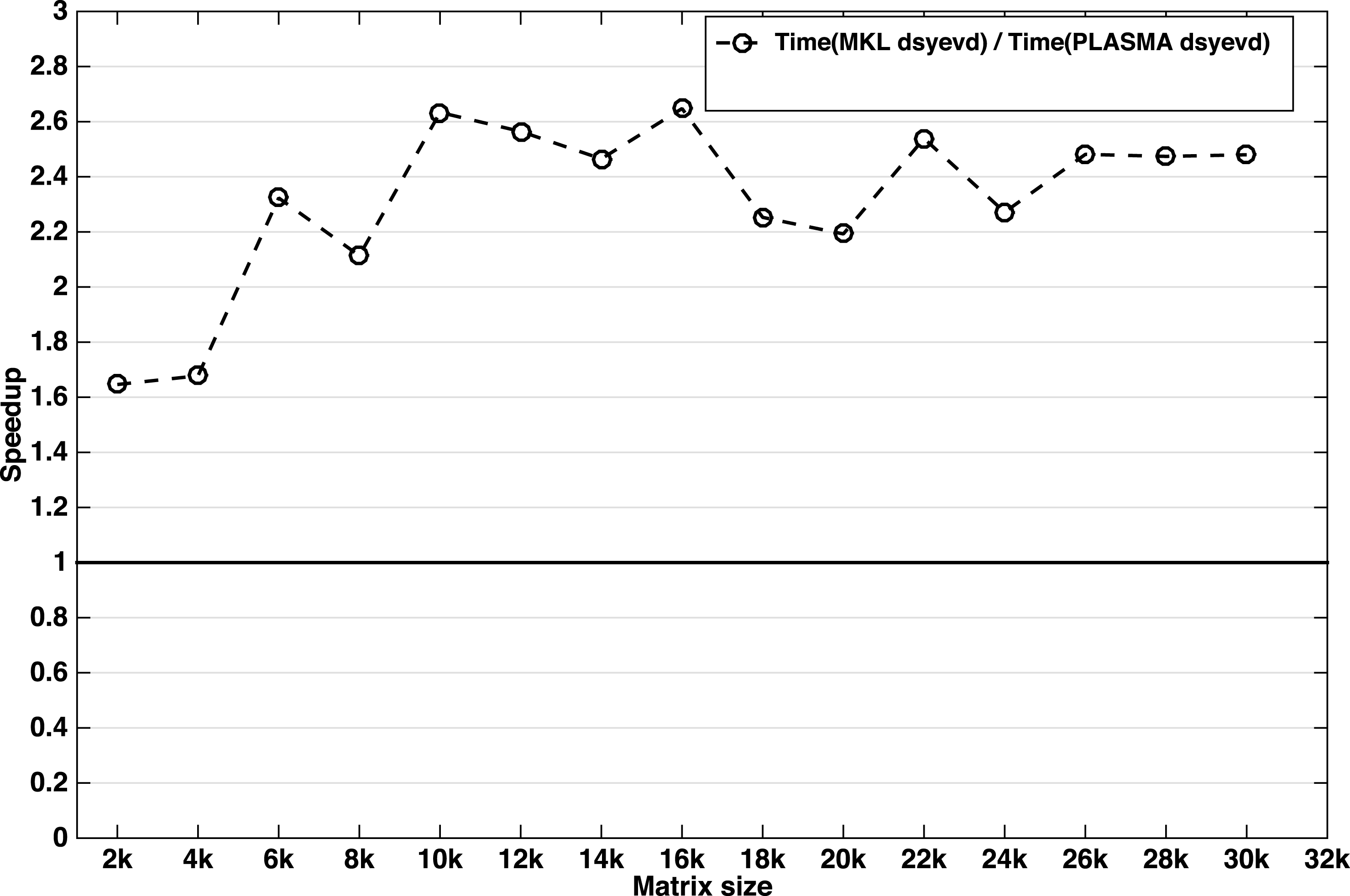
Below, we discuss the application of the Householder reflectors generated from the two stages of the reduction to tridiagonal form. The first stage reduces the original symmetric and/or Hermitian matrix  $A$ to a band matrix by applying a two-sided transformation to
 $A$ such that
 $A=Q_{1}A_{b}Q_{1}^{H}$. Similarly, the second stage, called bulge chasing, reduces the band matrix
 $B$ to the tridiagonal form by applying the transformation from both the left and right side of
 $A_{b}$ such that
 $A_{b}=Q_{2}TQ_{2}^{H}$. Thus, when the eigenvector matrix
 $X$ of
 $A$ is requested, the eigenvector matrix
 $Z$ that is produced by the eigensolver needs to be updated from the left by the two Householder reflectors generated during the reduction phase, according to the formula
 $$\begin{eqnarray}X=Q_{1}Q_{2}Z=(I-V_{1}T_{1}V_{1}^{H})(I-V_{2}T_{2}V_{2}^{H})Z,\end{eqnarray}$$
where ( $V_{1},T_{1}$) and (
 $V_{2},T_{2}$) represent the Householder reflectors generated during the first and second reduction stages, respectively. The application of the
 $V_{2}$ reflectors is not straightforward, while the application of the
 $V_{1}$ reflectors has to follow the tile fashion style. The same technique used for the singular value decomposition is used here as well. Thus, Algorithms 8 and 9 describe the procedure of applying
 $Q_{2}$ and
 $Q_{1}$, respectively. More details of the optimized technique can be found elsewhere (Haidar et al. Reference Haidar, Luszczek and Dongarra2014b). Both multiplications are based on Level 3 BLAS and are thus considered to perform very well on recent hardware, which alleviates the extra cost of the application of
 $Q_{2}$. The overall speedup and efficiency of this technique is demonstrated in the experimental results section below.
Speedup of our new two-stage implementation over the classic one-stage approach when only eigenvalues are computed using 28 Intel Xeon E5-2697 cores.
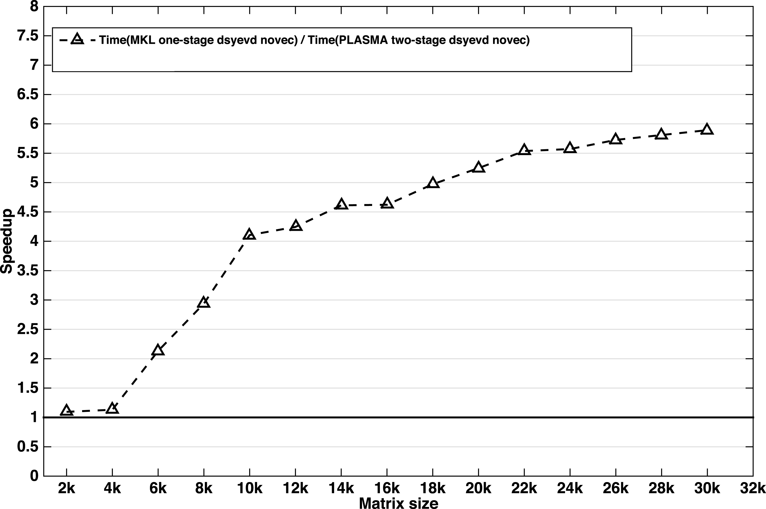
8.3.5 Experimental results
This section presents the performance comparisons of our tile algorithm for a two-stage symmetric eigenvalue solver against state-of-the-art numerical linear algebra libraries. To verify our findings in practice, we have performed the experiments on our two-socket multicore machine featuring a 14-core Intel Xeon E5-2697 processor in each socket running at 2.6 GHz, with 128 GB of main memory and 35 MB Level 2 cache. Figure 8.13 illustrates the speedup obtained by our two-stage approach over the classical one-stage implementation. The speedup curve shows that our two-stage algorithm outperforms the classical one-stage implementation by more than  $2\times$ when all eigenvalues and eigenvectors are needed.
When only the eigenvalues are needed, there is no extra cost related to updating the vectors, and thus we can expect a large speedup similar to that of the singular value decomposition. Figure 8.14 shows the obtained speedup from our experiments for eigenvalues only. The speedup obtained here is between  $5.5\times$ and
 $6\times$ faster when using the two-stage approach. In other words, the speedup varies depending on the portion of eigenvectors requested. For example, if 20% of the eigenvectors are needed, the last merge of our implementation of the divide and conquer algorithm can be modified to apply the update on only 20% of the vectors, thereby reducing the cost of the eigensolver by about 50%. The back transformation cost will be reduced by 80% for both the one-stage and two-stage approaches. The observed speedup in our experiment is about
 $4\times$ to
 $5\times$.
8.4 Non-symmetric eigenvalue problem
The non-symmetric eigenvalue problem revolves around finding scalar  ${\it\lambda}$ and vector
 $x$ such that
 $Ax={\it\lambda}x$, where
 $A$ is an
 $n\times n$ non-symmetric matrix. In addition to this left eigenvector
 $x$, there is also the right eigenvector
 $y$, such that
 $y^{T}A={\it\lambda}y^{T}$; in the symmetric case, these are identical. As in the symmetric case, the solution proceeds in three phases (Golub and Van Loan Reference Golub and Van Loan1996). First, the matrix is reduced to upper Hessenberg form by applying orthogonal
 $Q$ matrices on the left and right, to form
 $H=Q_{1}^{T}AQ_{1}$. The second phase, QR iteration, is an iterative process that reduces the Hessenberg matrix to upper triangular Schur form,
 $S=Q_{2}^{T}HQ_{2}$. Being based on similarity transformations, the eigenvalues of
 $A$ are the same as the eigenvalues of
 $S$, which are simply the diagonal elements of
 $S$. Finally, the third phase computes eigenvectors
 $Z$ of the Schur form
 $S$ and back-transforms them to eigenvectors
 $X$ of the original matrix
 $A$. The eigenvectors of
 $A$ are related to the eigenvectors of
 $S$ by multiplying with the orthogonal matrices used in the Hessenberg reduction and QR iteration as
 $X=Q_{1}Q_{2}Z$.
Execution time and operation count of LAPACK eigenvalue solver (DGEEV), annotated with parallel speedup for 16 cores.
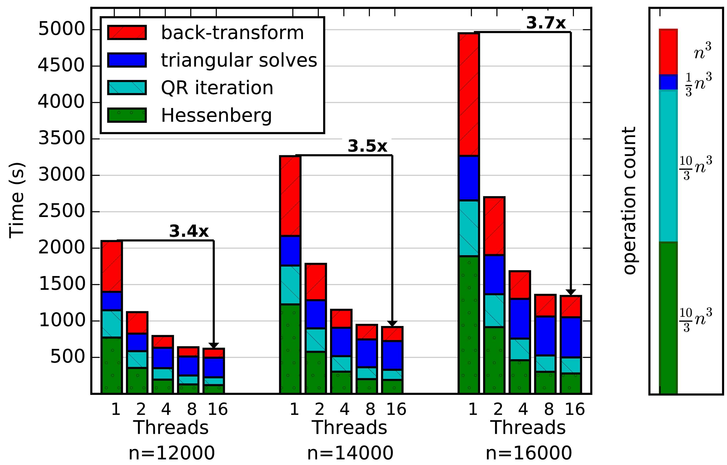
It is helpful to analyse the performance and scalability of an existing implementation in order to identify areas for improvement. A comparison of the floating-point operations (flops) and time for the LAPACK implementation is presented in Figure 8.15. The first phase, Hessenberg reduction, takes  $\frac{10}{3}n^{3}$ flops, and is formulated (Bischof Reference Bischof1993, Bischof and Van Loan Reference Bischof and Van Loan1987) so that
 $\frac{8}{3}n^{3}$ of these occur in efficient Level 3 BLAS matrix–matrix products (GEMM), while the remaining
 $\frac{2}{3}n^{3}$ occur in memory-bound Level 2 BLAS matrix–vector products (GEMV). Following the analysis in the symmetric case, performance is limited by the Level 2 BLAS operations, with a maximum performance
 $P_{\max }\leq 5P_{\text{GEMV}}$. There exists a two-stage implementation that reduces the amount of GEMV operations (Karlsson and Kågström Reference Karlsson and Kågström2011). However, a two-stage algorithm is more difficult than the symmetric problem. The first stage reduces to band Hessenberg, which still has
 $O(n^{2})$ entries, instead of a banded matrix with
 $O(n_{b}n)$ entries. This means that the second stage reduction from band Hessenberg to Hessenberg still takes
 $O(n^{3})$ time, instead of
 $O(n_{b}n^{2})$ time as in the symmetric case. Here, we concentrate on the classic one-stage algorithm. Asymptotically on 16 cores, the Hessenberg reduction takes 20% of the total time. The Hessenberg reduction is amenable to acceleration using a GPU or accelerator (Tomov, Nath and Dongarra Reference Tomov, Nath and Dongarra2010a), achieving a
 $3\times$ speedup over the 16-core CPU version.
The second phase, QR iteration, takes  $O(n^{3})$ flops, but being an iterative method, the exact count depends heavily on the convergence rate and techniques such as aggressive early deflation (Braman, Byers and Mathias Reference Braman, Byers and Mathias2002a, Reference Braman, Byers and Mathias2002b). Estimates range up to
 $25n^{3}$ flops (Golub and Van Loan Reference Golub and Van Loan1996), but we found that the flops decreased as the matrix size increased, and have measured it as low as
 $\frac{10}{3}n^{3}$ flops for large matrices, making its operation count similar to the Hessenberg reduction. QR iteration includes a mixture of Level 1 BLAS for applying Givens rotations and Level 3 BLAS for updating
 $H$ and accumulating
 $Q_{2}$. Parallel versions also exist (Kågström, Kressner and Shao Reference Kågström, Kressner, Shao and Jónasson2012). While for small matrices the QR iteration can take over 50% of the time, for large matrices this reduces to about 15% of the time on 16 cores.
The third phase, eigenvalue computation, computes each eigenvector of  $S$ by a triangular solve (LATRS), then back-transforms it to an eigenvector of
 $A$ with a matrix–vector product (GEMV). This phase takes
 $\frac{4}{3}n^{3}$ flops (
 $\frac{1}{3}n^{3}$ in triangular solves,
 $n^{3}$ in back-transformation), which is the least number of operations of the three phases. However, due to a lack of parallelization and involving only Level 2 BLAS operations, it has the lowest performance of the three phases in the LAPACK implementation. While the back-transformation achieves up to
 $6\times$ speedup with 16 cores, the specialized LATRS solver is not parallelized at all, limiting the eigenvector computation to
 $1.5\times$ speedup, and the overall speedup to
 $3.7\times$ on 16 cores, as seen in Figure 8.15. Due to the smaller speedup compared to the Hessenberg and QR iteration phases, its proportion increases to over 60% of the total time for large matrices using 16 cores. Thus, despite having the fewest operations of the three phases, the computation of eigenvectors has become the dominant cost and limited the overall parallel speedup of the solution of the eigenvalue problem. A parallel version of the eigenvector computation is available (Gates, Haidar and Dongarra Reference Gates, Haidar and Dongarra2014) that significantly improves its performance.
Here we cover recent work on accelerating the Hessenberg reduction phase using GPUs, improving the eigenvector computation phase by using Level 3 BLAS, and parallelizing the triangular solves with a task-based scheduler. Combined, these improvements significantly increase the performance and scalability of the overall eigenvalue problem.
8.4.1 Hessenberg reduction
Initially, the matrix  $A$ is reduced to an upper Hessenberg matrix
 $H$ using an orthogonal similarity transformation,
 $H=Q_{1}^{T}AQ_{1}$. The similarity transform preserves the eigenvalues, so
 $A$ and
 $H$ have the same eigenvalues, while using orthogonal matrices ensures good stability. Using elementary transformations based on an LU decomposition is also possible, which incurs half the floating-point operations as orthogonal matrices, but at reduced stability (Kabir, Haidar, Tomov and Dongarra Reference Kabir, Haidar, Tomov and Dongarra2015). The purpose of reducing the matrix to Hessenberg form is to reduce the operations in the second phase, QR iteration. From the Hessenberg form, only one sub-diagonal needs to be eliminated via QR iteration to achieve triangular Schur form.

Algorithm 11 presents a high-level view of the Hessenberg reduction. The reduction proceeds by introducing zeros below the sub-diagonal in each column  $a_{j}$ using a Householder transformation,
 $$\begin{eqnarray}H_{(j)}=I-{\it\tau}_{j}v_{j}v_{j}^{T}.\end{eqnarray}$$
As in the QR factorization in Section 5, instead of applying the Householder updates one by one using inefficient Level 2 BLAS operations, a blocked Householder transformation is used, where at step  $j$,
 $$\begin{eqnarray}Q_{(j)}=H_{(1)}H_{(2)}\cdots H_{(j)}=I-V_{(j)}T_{(j)}V_{(j)}^{T}\end{eqnarray}$$
with
 $$\begin{eqnarray}\displaystyle V_{(j)} & = & \displaystyle \left[\begin{array}{@{}c@{}}v_{1},\ldots ,v_{j}\end{array}\right],\nonumber\\ \displaystyle T_{(j)} & = & \displaystyle \left[\begin{array}{@{}cc@{}}T_{(j-1)} & -{\it\tau}_{j}T_{(j-1)}V_{(j-1)}^{T}v_{j}\\ 0 & {\it\tau}_{j}\end{array}\right].\nonumber\end{eqnarray}$$
The update to the trailing matrix of  $A$ is then
 $$\begin{eqnarray}\hat{A}=Q_{(j)}^{H}AQ_{(j)}=(I-V_{(j)}T_{(j)}^{H}V_{(j)}^{H})(A-Y_{(j)}T_{(j)}V_{(j)}^{H}),\end{eqnarray}$$
where
 $$\begin{eqnarray}Y_{(j)}=AV_{(j)}.\end{eqnarray}$$
While we delay updating the trailing matrix until accumulating a block of  $n_{b}$ Householder transformations, we must immediately update the next column of the panel with all previous transformations before we can compute its Householder transformation. For column
 $a_{j+1}$, this requires computing column
 $j+1$ of
 $Q_{(j)}^{H}AQ_{(j)}$. We can do this without computing the entire product, but it does require computing
 $y_{j}=Av_{j}$.
This matrix–vector product  $Av_{j}$ is a memory-bound, Level 2 BLAS operation that becomes a major bottleneck in the algorithm, limiting the maximum performance to
 $P_{\max }\leq 5P_{\text{GEMV}}$. To achieve higher performance, we utilize GPUs to accelerate both GEMV and GEMM operations. Because the GEMV is memory-bound, it benefits from the increased memory bandwidth available on the GPU, while the GEMM benefits from the high computational rate of the GPU.
The GPU implementation is shown in Algorithm 12; differences from the CPU-only algorithm occur in lines 3, 6, 7, 8, 16 and 17. The entire matrix is stored on the GPU. The current panel is copied to the CPU to be factored there. During the panel factorization, the vector  $v_{j}$ is sent to the GPU, where
 $y_{j}=Av_{j}$ is computed, and the resulting
 $y_{j}$ sent back to the CPU. After each panel factorization, the trailing matrix is updated on the GPU.
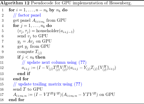
A multi-GPU implementation is also available. In this case, the matrix is distributed in a one-dimensional block-cyclic fashion across the GPUs. The GEMV is done independently on each GPU, with partial results sent to the CPU where a final summation is done. For instance, to compute  $y=Av$ using three GPUs,
 $$\begin{eqnarray}y=Av=\left[\begin{array}{@{}ccc@{}}A_{1} & A_{2} & A_{3}\end{array}\right]\left[\begin{array}{@{}c@{}}v_{1}\\ v_{2}\\ v_{3}\end{array}\right]=A_{1}v_{1}+A_{2}v_{2}+A_{3}v_{3}.\end{eqnarray}$$
Each GPU computes its part,  $A_{i}v_{i}$, which are then sent to the CPU to be summed for the final result,
 $y$. After the panel factorization, the
 $V$,
 $Y$, and
 $T$ matrices are replicated on all the GPUs, then each GPU updates its portion of the trailing matrix. Figure 8.16 shows the performance of the multi-GPU version compared to Intel MKL running on two 8-core CPUs. A single GPU achieves a
 $3.3\times$ speedup over the CPU-only version, while three GPUs achieve up to a
 $9.2\times$ speedup. This shows good parallel speedup, with three GPUs being
 $2.8\times$ faster than a single GPU. The
 $P_{\max }<5P_{\text{GEMV}}$ bound is also shown in Figure 8.16 for both CPU and GPU. The GPU GEMV achieves 45.6 Gflops, while the CPU GEMV achieves up to 14.7 Gflops. On the GPU, the Hessenberg achieves 77% of the bound, while on the CPU, it achieves 72% of the bound.
Execution time of Hessenberg reduction (DGEHRD) using two 8-core CPUs and up to three NVIDIA Kepler K40 GPUs. Dashed lines indicate performance bound,  $P_{\max }=5P_{\text{GEMV}}$, for CPU and single GPU implementations.
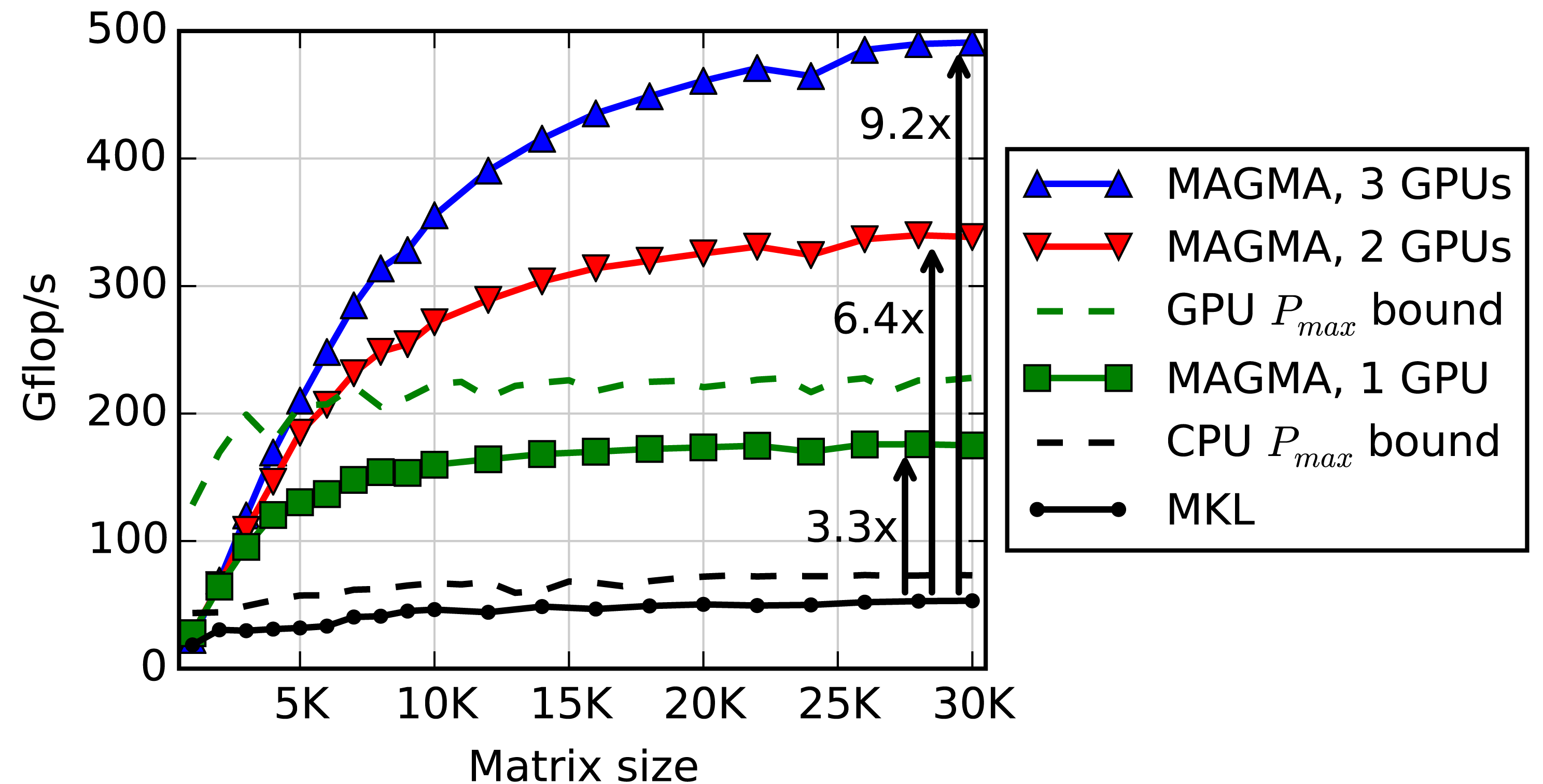
8.4.2 Eigenvector computation
When eigenvectors are desired, the third phase computes eigenvectors of the triangular Schur form  $S$, then back-transforms them to eigenvectors of the original matrix
 $A$. In LAPACK, this phase is implemented in the TREVC (triangular eigenvector computation) routine. We will assume only right eigenvectors are desired, but the computation of left eigenvectors is similar and amenable to the same techniques as described here. After the Hessenberg and QR iteration phases, the diagonal entries of
 $S$ are the eigenvalues
 ${\it\lambda}_{k}$ of
 $A$. To determine the corresponding eigenvectors, we solve
 $Sz_{k}={\it\lambda}_{k}z_{k}$ by considering the decomposition (Golub and Van Loan Reference Golub and Van Loan1996)
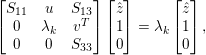 $$\begin{eqnarray}\left[\begin{array}{@{}ccc@{}}S_{11} & u & S_{13}\\ 0 & {\it\lambda}_{k} & v^{T}\\ 0 & 0 & S_{33}\\ \end{array}\right]\left[\begin{array}{@{}c@{}}\hat{z}\\ 1\\ 0\\ \end{array}\right]={\it\lambda}_{k}\left[\begin{array}{@{}c@{}}\hat{z}\\ 1\\ 0\\ \end{array}\right],\end{eqnarray}$$
which yields  $(S_{11}-{\it\lambda}_{k}I)\hat{z}=-u$. Thus computing each eigenvector
 $z_{k}$ of
 $S$ involves a
 $k-1\times k-1$ triangular solve, for
 $k=2,\ldots ,n$. Each solve has a slightly different
 $S$ matrix, with the diagonal modified by subtracting
 ${\it\lambda}_{k}$. The resulting eigenvector
 $z_{k}$ of
 $S$ must then be back-transformed by multiplying with the
 $Q$ formed in the Hessenberg and QR iteration phases to get the eigenvector
 $x_{k}=Qz_{k}$ of the original matrix
 $A$.
Note that if two eigenvalues,  ${\it\lambda}_{k}$ and
 ${\it\lambda}_{j}$ (
 $k>j$), are identical, then
 $S_{11}-{\it\lambda}_{k}I$ is singular. More generally,
 $S_{11}-{\it\lambda}_{k}I$ can be badly conditioned. Therefore, instead of using the standard BLAS triangular solver (TRSV), a specialized triangular solver (LATRS) is used, which scales columns to protect against overflow, and can generate a consistent solution for a singular matrix.
This method works in complex arithmetic, but the case in real arithmetic is more complicated. For a real matrix  $A$, the eigenvalues can still be complex, coming in conjugate pairs,
 ${\it\lambda}_{k}$ and
 $\bar{{\it\lambda}}_{k}$. The eigenvectors are likewise conjugate pairs,
 $z_{k}$ and
 $\bar{z}_{k}$. In real arithmetic, the closest that QR iteration can come to triangular Schur form is quasi-triangular real Schur form, which has a
 $2\times 2$ diagonal block for each conjugate pair of eigenvalues. A specialized quasi-triangular solver is required, which factors each
 $2\times 2$ diagonal block, and protects against overflow and dealing with singular matrices. In LAPACK this solver is implemented inline as part of the DTREVC routine.
8.4.3 Blocking back-transformation
Our first step to improve the eigenvector computation is to block the  $n$GEMV operations for the back-transformation into
 $n/n_{b}$GEMM operations, where
 $n_{b}$ is the block size. This requires two
 $n\times n_{b}$ workspaces: one for the vectors
 $z_{k}$, the second for the back-transformed vectors
 $x_{k}$ before copying to the output
 $V$.
Pseudocode for the blocked back-transformation is shown in Algorithm 13 along with the parallel solver described in Section 8.4.4. For each block, we loop over  $n_{b}$ columns, performing a triangular solve for each column and storing the resulting eigenvectors
 $z_{k}$ in workspace
 $Z$. After filling up
 $n_{b}$ columns of
 $Z$, a single GEMM back-transforms all
 $n_{b}$ vectors, storing the result in workspace
 $\tilde{Z}$. The vectors are then normalized and copied to
 $V$. On input, the matrix
 $V=Q$. Recall from equation (8.11) that the bottom
 $n-k$ rows of eigenvector
 $z_{k}$ are 0, so the last
 $n-k$ columns of
 $Q$ are not needed for the GEMM. Therefore, we start from
 $k=n$ and work down to
 $k=1$, writing each block of eigenvectors to
 $V$ over columns of
 $Q$ after they are no longer needed.

The real case is similar, but has the minor complication that complex conjugate pairs of eigenvalues will generate conjugate pairs of eigenvectors,  $z_{k}=a+bi$ and
 $\bar{z}_{k}=a-bi$, which are stored as two columns,
 $a$ and
 $b$, in
 $Z$. When the first eigenvalue of each pair is encountered, both columns are computed; then the next eigenvalue (its conjugate) is skipped. Once
 $n_{b}-1$ columns are processed, if the next eigenvector is complex it must be delayed until the next block.
8.4.4 Multithreading triangular solver
After blocking the back-transform, the triangular solver remains a major bottleneck because it is not parallelized. Recall that the triangular matrix being solved is different for each eigenvector – the diagonal is modified by subtracting  ${\it\lambda}_{k}$. This prevents blocking and solving multiple eigenvectors together using a Level 3 BLAS DTRSM operation.
In the complex case, LAPACK’s ZTREVC uses a safe triangular solver, ZLATRS. Unlike the standard ZTRSV BLAS routine, ZLATRS uses column scaling to avoid numerical instability, and handles singular triangular matrices. Therefore, to avoid jeopardizing the accuracy or stability of the eigensolver, we continue to rely on ZLATRS instead of the optimized, multithreaded ZTRSV. However, processing  $S$ column by column prevents parallelizing individual calls to ZLATRS, as is typically done for BLAS functions. Instead, we observe that multiple triangular solves could occur in parallel. One obstacle is that a different
 ${\it\lambda}_{k}$ is subtracted from the diagonal in each case, modifying
 $S$ in memory. Our solution is to write a modified routine, ZLATRSD (triangular solve with modified diagonal), which takes both the original unmodified
 $S_{11}$ and the
 ${\it\lambda}_{k}$ to subtract from the diagonal. The subtraction is done as the diagonal elements are used, without modifying
 $S$ in memory. This allows us to pass the same
 $S$ to each ZLATRSD call and hence solve multiple eigenvectors in parallel, one in each thread.
As previously mentioned, the real case requires a special quasi-triangular solver to solve each  $2\times 2$ diagonal block. In the original LAPACK code, this quasi-triangular solver is embedded in the DTREVC routine. To support multithreading, we refactor it into a new routine, DLAQTRSD, a quasi-triangular solver with modified diagonal. Unlike the complex case, instead of passing
 ${\it\lambda}_{k}$ separately, DLAQTRSD computes it directly from the diagonal block of
 $S$. If
 ${\it\lambda}_{k}$ is real, DLAQTRSD computes a single real eigenvector. If
 ${\it\lambda}_{k}$ is one of a complex conjugate pair, DLAQTRSD computes a complex eigenvector as two real vectors.
To deal with multithreading, we use a thread pool design pattern. As shown in Algorithm 13, the main thread inserts LATRSD tasks into a queue. Worker threads pull tasks out of the queue and execute them. For this application, there are no dependencies to be tracked between the triangular solves. After a block of  $n_{b}$ vectors has been computed, we back-transform them with a GEMM. We could call a multithreaded GEMM, as available in MKL, but to simplify thread management, we found it more suitable to use the same thread pool for the GEMM as for LATRSD. For
 $p$ threads, the GEMM is split into
 $p$ tasks, each task multiplying a single block row of
 $Q$ with
 $Z$. After the GEMM, the next block of
 $n_{b}$ vectors is computed. Within each thread, the BLAS calls are single-threaded.
8.4.5 Using accelerators
To further accelerate the eigenvector computation, we observe that the triangular solves and the back-transformation GEMM can be done in parallel. In particular, the GEMM can be done on a GPU while the CPU performs the triangular solves. Data transfers can also be done asynchronously and overlapped with the triangular solves. To facilitate this asynchronous computation, we double-buffer the CPU workspace  $Z$, using it to store results from LATRSD, then swap with
 $\tilde{Z}$, which is used to send data to the GPU while the next block of LATRSD solves are performed with
 $Z$. The difference from Algorithm 13 is shown in Algorithm 14.

8.4.6 Results
We performed tests with two 8-core, 2.6 GHz Intel E5-2670 CPUs and an 875 MHz NVIDIA K40 GPU, with Intel MKL 11.0.5 for optimized, multithreaded BLAS. Matrices were double precision with uniform random entries in  $(0,1)$. Inside our parallel TREVC, we launch
 $p$ Pthreads and set MKL to be single-threaded; outside TREVC, MKL uses the same number of threads,
 $p$.
Figure 8.17 shows the total eigenvalue problem (DGEEV) time, broken down into four phases: Hessenberg reduction (lowest tier), QR iteration (second tier), triangular solves (third tier), and back-transformation (top tier). The triangular solves and back-transformation together form the eigenvector computation. Columns are grouped by the matrix size. We compare results to the LAPACK reference implementation in Intel MKL.
Execution time of eigenvalue solver (DGEEV) using 16 cores, annotated with cumulative speedup with each improvement.
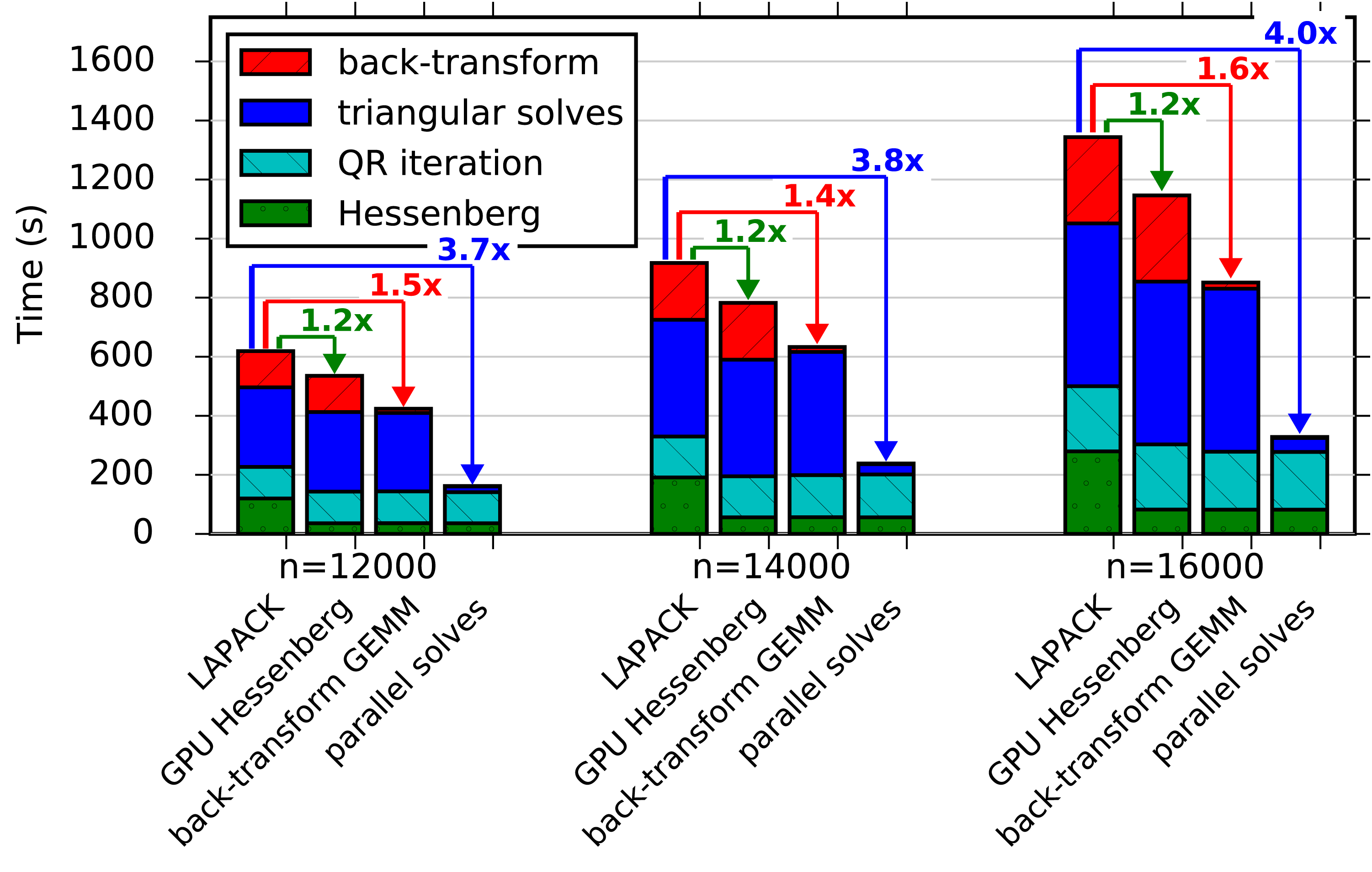
The improvement gained from accelerating the Hessenberg on a single GPU is shown in the second column of each group in Figure 8.17. The Hessenberg itself is up to  $3.3\times$ faster, shown earlier in Figure 8.16. However, it is only 20% of the total time, so the overall speedup of DGEEV is only
 $1.2\times$, shown in Figure 8.17 and by the diamonds in Figure 8.19.
Blocking the back-transformation with a GEMM is shown in the third column of each group in Figure 8.17. The GEMM itself is up to  $14\times$ faster than the non-blocked back-transformation using 16 threads. Further, the solid line with squares in Figure 8.18 shows it has better parallel scaling, reaching a speedup of
 $12\times$ for 16 cores, compared to only
 $6\times$ for the LAPACK implementation. However, as the triangular solves are not yet parallelized, the overall eigenvalue problem improvement is limited, being at most
 $1.6\times$ faster, as seen in Figure 8.17.
Parallel speedup of individual phases, for  $p=16$ versus
 $p=1$.
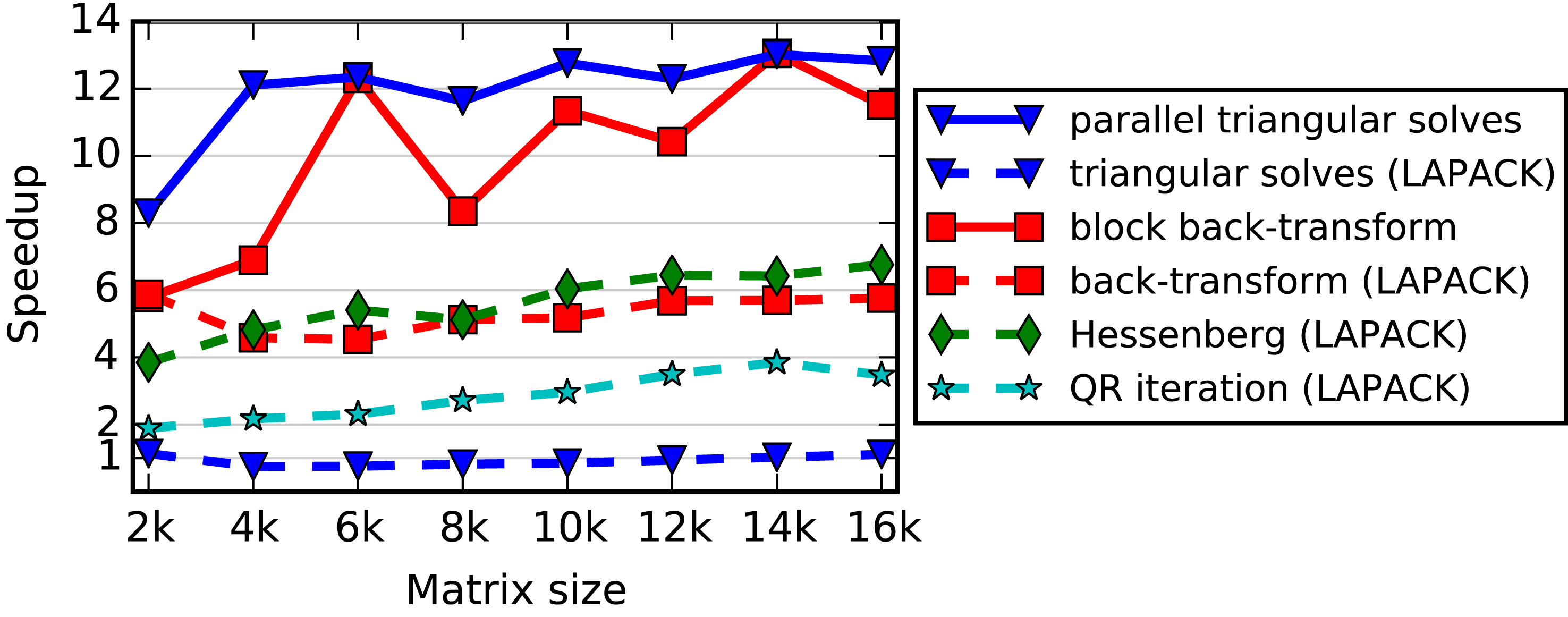
Overall improvement of eigenvalue solver (DGEEV) compared to LAPACK, after various improvements, using  $p=16$ threads.
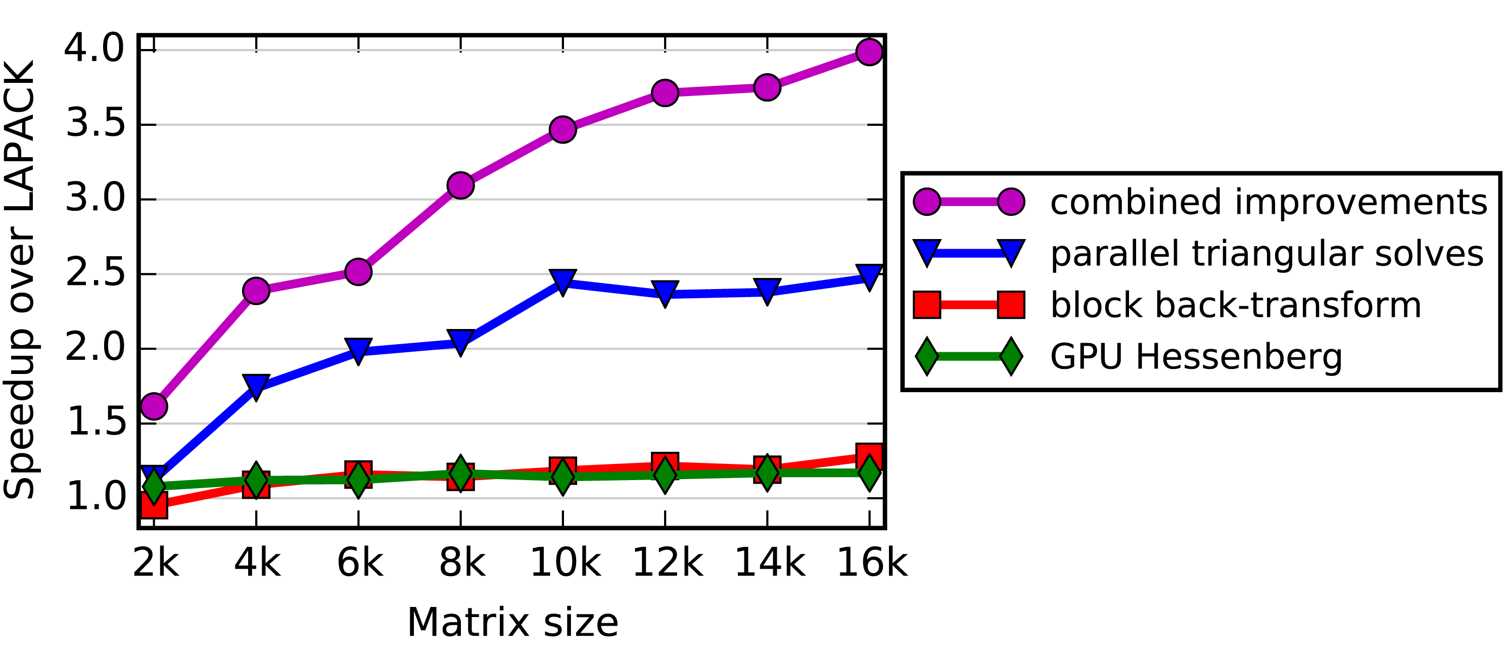
Parallelizing the triangular solves is the fourth column of each group in Figure 8.17. With multiple threads, we see significant parallel speedup, up to  $12.8\times$ for 16 threads, shown by the triangles in Figure 8.18. Combined with the GPU-accelerated Hessenberg and the blocked back-transformation, these three modifications significantly improve the solution of the overall eigenvalue problem by up to
 $4\times$ for 16 cores, shown by the circles in Figure 8.19, and annotated in Figure 8.17.
Thus, we see that different strategies are used to accelerate different portions of the computation – a combination of GPU acceleration, blocking into Level 3 BLAS operations, and parallelizing Level 2 BLAS operations. Ignoring any one portion yields mediocre results, while addressing both the Hessenberg reduction and the eigenvector computation phases yields substantial improvements. The bottleneck is now moved back to QR iteration, which is natural as it has the most operations and its iterative nature makes it the most complicated and difficult phase to parallelize.
9 Mixed precision algorithms
On modern architectures, single precision 32-bit floating-point arithmetic (FP32) is usually twice as fast as double precision 64-bit floating-point arithmetic (FP64). The reason for this is that the number of bytes moved through the memory system is essentially halved. Indeed, on most current multicore CPUs, high-end AMD GPUs (e.g. FirePro W9100), and Intel Xeon Phi, the single precision peak is twice the double precision peak. On most high-end NVIDIA GPUs (e.g. the GeForce GTX Titan Black) the ratio of single precision peak versus double precision peak is  $3\times$ more, but can go up to
 $32\times$ (e.g. on the Titan X) depending on the ratio of 32-bit to 64-bit CUDA cores.
Single precision is not the best answer for all applications, however. For example, several physics applications require 64-bit accuracy (double precision) to be maintained throughout the computation, and 32-bit accuracy (single precision) is simply not an option. The obvious reason is that in order for the application to give an accurate answer, it needs the highest precision. Also, 64-bit accuracy enables most of the modern computational methods to be more stable; therefore, in mission-critical applications, one must use 64-bit accuracy to obtain an answer. However, as stated above, the raw performance of 32-bit single precision is too tempting to ignore, and here we present a methodology of how to perform the bulk of the operations in 32-bit arithmetic, then postprocess the 32-bit solution by refining it into a solution that is 64-bit accurate. We present this methodology in the context of solving a system of linear equations, be it sparse or dense, symmetric positive definite or non-symmetric, using either direct or iterative methods. We believe that the approach outlined below is quite general and should be considered by application developers for their practical problems.
9.1 The idea behind mixed precision algorithms
Mixed precision algorithms stem from the observation that, in many cases, a single precision solution of a problem can be refined to the point where double precision accuracy is achieved. The refinement can be accomplished, for instance, by means of the Newton’s algorithm (Ypma Reference Ypma1995) which computes the zero of a function  $f(x)$ according to the iterative formula
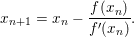 $$\begin{eqnarray}x_{n+1}=x_{n}-\frac{f(x_{n})}{f^{\prime }(x_{n})}.\end{eqnarray}$$
In general, we would compute a starting point and  $f^{\prime }(x)$ in single precision arithmetic and the refinement process would be computed in double precision arithmetic.
If the refinement process is cheaper than the initial computation of the solution, then double precision accuracy can be achieved nearly at the same speed as the single precision accuracy. The two following subsections describe how this concept can be applied to solvers of linear systems based on direct and iterative methods, respectively.
9.1.1 Direct methods
A common approach to the solution of linear systems, either dense or sparse, is to perform the LU factorization of the coefficient matrix using Gaussian elimination. First, the coefficient matrix  $A$ is factored into the product of a lower triangular matrix
 $L$ and an upper triangular matrix
 $U$. Partial row pivoting is, in general, used to improve numerical stability resulting in a factorization
 $PA=LU$, where
 $P$ is a permutation matrix. The solution for the system is achieved by first solving
 $Ly=Pb$ (forward substitution) and then solving
 $Ux=y$ (backward substitution). Due to round-off errors, the computed solution
 $x$ carries a numerical error magnified by the condition number of the coefficient matrix
 $A$.
In order to improve the computed solution, we can apply an iterative process which produces a correction to the computed solution at each iteration, which then yields the method that is commonly known as the iterative refinement algorithm. As Demmel (Reference Demmel1997) points out, the non-linearity of the round-off errors makes iterative refinement equivalent to Newton’s method applied to the function  $f(x)=b-Ax$. Provided that the system is not too ill-conditioned, the algorithm produces a solution correct for the working precision. Iterative refinement in double–double precision is a fairly well-understood concept and was analysed by Wilkinson (Reference Wilkinson1963), Moler (Reference Moler1967) and Stewart (Reference Stewart1973).
The algorithm can be modified to use a mixed precision approach. The factorization  $PA=LU$, the solution of the triangular systems
 $Ly=Pb$, and
 $Ux=y$ are computed using single precision arithmetic. The residual calculation and the update of the solution are computed using double precision arithmetic and the original double precision coefficients: see Algorithm 15. The most computationally expensive operation, the factorization of the coefficient matrix
 $A$, is performed using single precision arithmetic and takes advantage of its higher speed. The only operations that must be executed in double precision are the residual calculation and the update of the solution (denoted by
 ${\it\varepsilon}_{d}$ in Algorithm 15). We observe that the only operation with computational complexity of
 $O(n^{3})$ is handled in single precision, while all operations performed in double precision are of at most
 $O(n^{2})$ complexity. The coefficient matrix
 $A$ is converted to single precision for the LU factorization and the resulting factors are stored in single precision while the initial coefficient matrix
 $A$ needs to be kept in memory. Therefore, one drawback of the following approach is that it uses 50% more memory than the standard double precision algorithm.
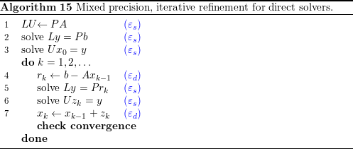
The method in Algorithm 15 can offer significant improvements for the solution of a sparse linear system in many cases.
1 Single precision computation is significantly faster than double precision computation.
2 The iterative refinement procedure converges in a small number of steps.
3 The cost of each iteration is small compared to the cost of the system factorization. If the cost of each iteration is too high, then a low number of iterations will result in a performance loss with respect to the full double precision solver. In the sparse case, for a fixed matrix size, both the cost of the system factorization and the cost of the iterative refinement step may vary substantially depending on the number of non-zeros and the matrix sparsity structure. In the dense case, results are more predictable.
Note that the choice of the stopping criterion in the iterative refinement process is critical. Formulas for the error computed at each step of Algorithm 15 can be obtained, for instance, in Oettli and Prager (Reference Oettli and Prager1964) and Demmel et al. (Reference Demmel, Hida, Kahan, Li, Mukherjee and Riedy2006).
9.1.2 Iterative methods
Direct methods are usually a very robust tool for the solution of sparse linear systems. However, they suffer from fill-in, which results in high memory requirements, long execution time, and non-optimal scalability in parallel environments. To overcome these limitations, various pivot reordering techniques are commonly applied to minimize the amount of generated fill-in and to enable better exploitation of parallelism. Still, there are cases where direct methods pose too high a memory requirement or deliver poor performance. Iterative methods are a valid alternative even though they are less robust and have less predictable behaviour. Iterative methods do not require more memory than is needed for the original coefficient matrix. Furthermore, time to solution can be better than that of direct methods if convergence is achieved in relatively few iterations (Barrett et al. Reference Barrett, Berry, Chan, Demmel, Donato, Dongarra, Eijkhout, Pozo, Romine and van der Vorst1994a, Saad Reference Saad2003).
In the context of iterative methods, the refinement method outlined in Algorithm 15 can be represented as
 $$\begin{eqnarray}x_{i+1}=x_{i}+M(b-Ax_{i}),\end{eqnarray}$$
where  $M$ is
 $(LU)^{-1}P$. Note that in this case
 $M$ approximates
 $A^{-1}$, which makes it known, in the area of linear algebra and numerical analysis, as a preconditioner of
 $A$. The preconditioner should approximate
 $A^{-1}$, and the quality of the approximation determines the convergence properties of the iterative solver. In general, a preconditioner is intended to improve the robustness and the efficiency of iterative methods. Note that (9.2) can also be interpreted as a Richardson method’s iteration in solving
 $MAx=Mb$, which is called left preconditioning. An alternative is to use right preconditioning, whereby the original problem
 $Ax=b$ is transformed into a problem of solving
 $$\begin{eqnarray}AMu=b,\quad x=Mu\end{eqnarray}$$
iteratively. Later on, we will use right preconditioning for mixed precision iterative methods.
 $M$ needs to be easy to compute, apply, and store to guarantee the overall efficiency. Note that these requirements were addressed in the mixed precision direct methods above by replacing
 $M$ (coming from LU factorization of
 $A$ followed by matrix inversion) with its single precision representation so that arithmetic operations can be performed more efficiently on it. Here, however, we go two steps further. We not only replace
 $M$ with an inner loop, which is an incomplete iterative solver working in single precision arithmetic (Turner and Walker Reference Turner and Walker1992), but we also replace the outer loop with a more sophisticated iterative method (e.g. based on Krylov subspace).
Note that replacing  $M$ with an iterative method leads to nesting of two iterative methods. Variations of this type of nesting, also known in the literature as an inner–outer iteration, have been studied, both theoretically and computationally (Golub and Ye Reference Golub and Ye2000, Saad Reference Saad1993, Simoncini and Szyld Reference Simoncini and Szyld2003, Axelsson and Vassilevski Reference Axelsson and Vassilevski1991, Notay Reference Notay2000, Vuik Reference Vuik1995, van den Eshof, Sleijpen and van Gijzen Reference van den Eshof, Sleijpen and van Gijzen2005). The general appeal of these methods is that the computational speedup hinges on the inner solver’s ability to use an approximation of the original matrix
 $A$ that is fast to apply. In our case, we use single precision matrix–vector products as a fast approximation of the double precision operator in the inner iterative solver. Moreover, even if no faster matrix–vector product is available, speedup can often be observed due to improved convergence (see e.g. Simoncini and Szyld Reference Simoncini and Szyld2003, who explain the possible benefits of FGMRES–GMRES over restarted GMRES).
To illustrate the above concepts, we demonstrate an inner–outer non-symmetric iterative solver in mixed precision. The solver is based on restarted generalized minimal residual (GMRES). In particular, consider Algorithm 16, where the outer loop uses flexible GMRES (FGMRES: Saad Reference Saad1993, Reference Saad2003) and the inner loop uses GMRES in single precision arithmetic (GMRES $_{\text{SP}}$). FGMRES, being a minor modification of standard GMRES, is meant to accommodate non-constant preconditioners. Note that in our case this non-constant preconditioner is GMRES
 $_{\text{SP}}$. The resulting method is denoted by FGMRES(
 $m_{\text{out}}$)–GMRES
 $_{\text{SP}}$(
 $m_{\text{in}}$), where
 $m_{\text{in}}$ is the restart for the inner loop and
 $m_{\text{out}}$ for the outer FGMRES. Algorithm 16 checks for convergence at every
 $m_{\text{out}}$ outer iterations, but an actual implementation can check for convergence at every inner iteration with simple tricks, for almost no computational cost.

The potential benefits of FGMRES compared to GMRES are becoming better understood (Simoncini and Szyld Reference Simoncini and Szyld2003). Numerical experiments confirm improvements in speed, robustness, and sometimes memory requirements for these methods (Buttari et al. Reference Buttari, Dongarra, Kurzak, Luszczek and Tomov2008a, Baboulin et al. Reference Baboulin, Buttari, Dongarra, Kurzak, Langou, Langou, Luszczek and Tomov2009). The memory requirements for the method are the matrix  $A$ in CRS format, the non-zero matrix coefficients in single precision,
 $2\,m_{\text{out}}$ number of vectors in double precision, and
 $m_{\text{in}}$ number of vectors in single precision.
The generalized conjugate residuals (GCR) method (Vuik Reference Vuik1995, van der Vorst and Vuik Reference van der Vorst and Vuik1994) is a possible replacement for FGMRES as the outer iterative solver. It is not yet well understood whether one should choose GCR or FGMRES.
As in the dense case, the choice of the stopping criterion in the iterative refinement process is critical. In the sparse case, formulas for the errors can be computed following the work of Arioli, Demmel and Duff (Reference Arioli, Demmel and Duff1989).
9.2 Performance results
Based on backward stability analysis, the solution  $x$ can be considered as accurate as the double precision one when
 $$\begin{eqnarray}\Vert b-Ax\Vert _{2}\leq \Vert x\Vert _{2}\cdot \Vert A\Vert _{2}\cdot {\it\varepsilon}\cdot \sqrt{n},\end{eqnarray}$$
where  $\Vert \cdot \Vert _{2}$ is the spectral norm.
9.2.1 Direct methods
The mixed precision iterative refinement solvers for dense matrices are available in LAPACK (Anderson et al. Reference Anderson, Bai, Bischof, Blackford, Demmel, Dongarra, Ducroz, Greenbaum, Hammarling, McKenney and Sorensen1999). For the non-symmetric case, step 1 in Algorithm 15 is implemented by means of the SGETRF subroutine, steps 2, 3 and 5, 6 with the SGETRS subroutine, step 4 with the DGEMM subroutine, and step 7 with the DAXPY subroutine. For the symmetric case the SGETRF, SGETRS, and DGEMM subroutines were replaced by the SPOTRF, SPOTRS, and DSYMM subroutines, respectively. Further details of these implementations can be found in Langou et al. (Reference Langou, Langou, Luszczek, Kurzak, Buttari and Dongarra2006) and Buttari et al. (Reference Buttari, Dongarra, Langou, Langou, Luszczek and Kurzak2007).
As already mentioned, iterative refinement solvers require  $1.5\times$ as much memory as a regular double precision solver, because the mixed precision iterative refinement solvers need to store both the single precision and the double precision versions of the coefficient matrix at the same time. This applies to both dense and sparse matrices.
Numerical results show that on older single-core architectures – such as the AMD Opteron, Intel Woodcrest, or IBM PowerPC – the mixed precision iterative solver could provide a speedup of up to  $1.8\times$ for the non-symmetric solver and
 $1.5\times$ for the symmetric solver for sufficiently large problem sizes (Baboulin et al. Reference Baboulin, Buttari, Dongarra, Kurzak, Langou, Langou, Luszczek and Tomov2009). For small problem sizes, the cost of even a few iterative refinement iterations is high compared to the cost of the factorization, and thus the mixed precision iterative solver is less efficient than the double precision solver (Baboulin et al. Reference Baboulin, Buttari, Dongarra, Kurzak, Langou, Langou, Luszczek and Tomov2009).
The mixed precision iterative refinement solvers were ported and optimized for multicore architectures in the PLASMA library. On the STI Cell BE architecture, for example, where the peak for single precision operations was  $14\times$ higher than the peak for double precision operations, the mixed precision solver performed up to
 $7\times$ faster than the double precision peak in the non-symmetric case and
 $11\times$ faster for the symmetric positive definite case. Implementation details for this case can be found in Kurzak and Dongarra (Reference Kurzak and Dongarra2007) and Kurzak, Buttari and Dongarra (Reference Kurzak, Buttari and Dongarra2008).
Mixed precision, iterative refinement method from MAGMA 1.6.2 for the solution of dense linear systems on the NVIDIA’s TITAN X GPU.
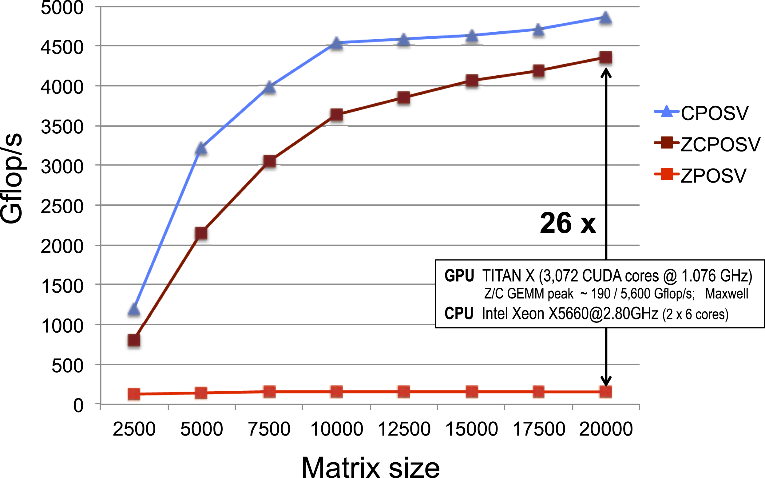
Parallel implementations of Algorithm 15 have been available for GPUs since MAGMA’s 0.2 release (Tomov, Nath, Du and Dongarra Reference Tomov, Nath, Du and Dongarra2009). Figure 9.1 illustrates the performance of MAGMA 1.6.2 on a Titan X GPU. Due to the  $32\times$ difference between the speed of FP32 and FP64 on this GPU, the mixed precision solver performs up to
 $26\times$ faster than the double precision peak. Implementation details can be obtained from the MAGMA sources.Footnote 6 Results on older GPUs, including the use of multiple GPUs, can be found in Tomov, Nath, Ltaief and Dongarra (Reference Tomov, Nath, Ltaief and Dongarra2010b).
For sparse matrices, the methodology can be applied using sparse direct methods: with either multifrontal (Duff and Reid Reference Duff and Reid1983) or supernodal (Ashcraft et al. Reference Ashcraft, Grimes, Lewis, Peyton and Simon1987) factorization approaches. For results on supernodal solvers see Buttari et al. (Reference Buttari, Dongarra, Kurzak, Luszczek and Tomov2008a). For multifrontal solvers, there are a number of freely available packages. The use of MUMPS (Amestoy, Duff and L’Excellent Reference Amestoy, Duff and L’Excellent2000, Amestoy, Duff, L’Excellent and Koster Reference Amestoy, Duff, L’Excellent and Koster2001, Amestoy, Guermouche, L’Excellent and Pralet Reference Amestoy, Guermouche, L’Excellent and Pralet2006), for example, comprises three separate steps.
1 System analysis. In this phase the system sparsity structure is analysed in order to estimate the element fill-in, which provides an estimate of the memory that will be allocated in the following steps. Also, pivoting is performed based on the structure of
$A+A^{T}$, ignoring numerical values. Only integer operations are performed at this step.2 Matrix factorization. In this phase the
$PA=LU$ factorization is performed. Computationally, this is the most expensive step of the system solution.3 System solution. The system is solved in two steps,
$Ly=Pb$ and $Ux=y$.


The first and second phases correspond to step 1 in Algorithm 15, while the third phase corresponds to steps 2, 3 and 5, 6.
Performance improvements for direct sparse methods when going from a full double precision solve (reference time) to a mixed precision solve.
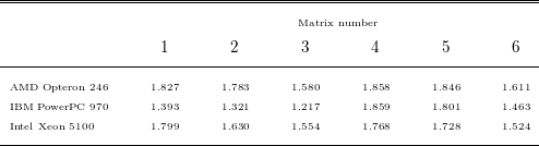
Table 9.1 shows the speedup of the mixed precision iterative refinement approach over the double precision approach for sparse direct methods, using the matrices described in Table 9.2.
Test matrices for sparse mixed precision, iterative refinement solution methods.
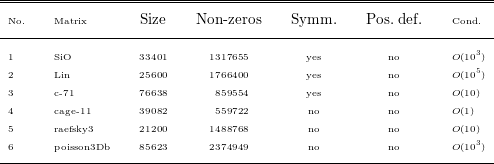
9.2.2 Iterative methods
Similar to the case of sparse direct solvers, we demonstrate the numerical performance of Algorithm 16 on the matrices from Table 9.2.
Mixed precision iterative refinement with FGMRES–GMRES $_{\text{SP}}$ from Algorithm 16 versus FGMRES–GMRES
 $_{\text{DP}}$.
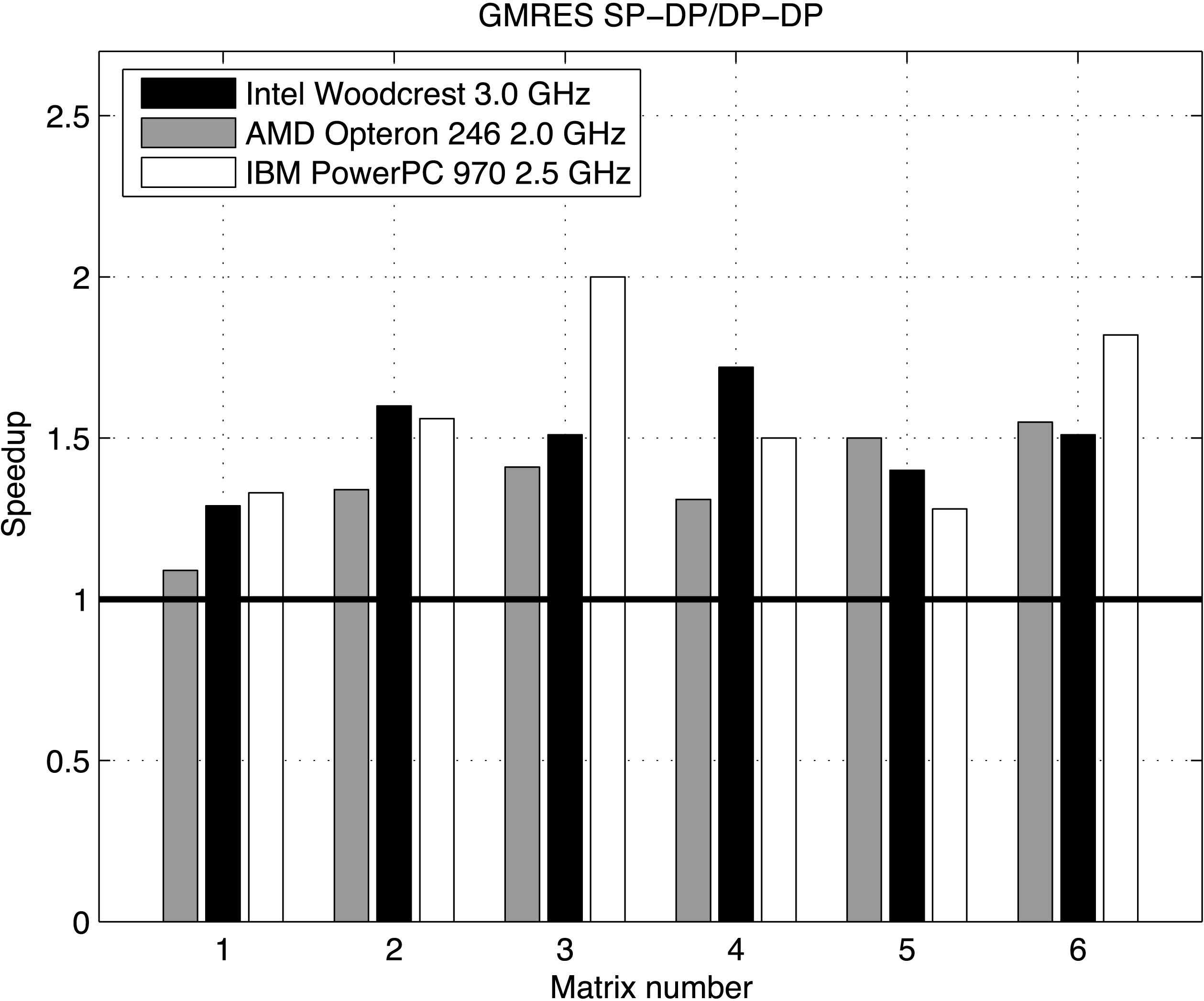
Figure 9.2 shows the performance ratio of the mixed precision inner–outer FGMRES–GMRES $_{\text{SP}}$ versus the full double precision inner–outer FGMRES–GMRES
 $_{\text{DP}}$. In other words, we compare two inner–outer algorithms that are virtually the same. The only difference is that their inner loop’s incomplete solvers are performed in single and double precision arithmetic.
For further details see Baboulin et al. (Reference Baboulin, Buttari, Dongarra, Kurzak, Langou, Langou, Luszczek and Tomov2009), which includes an experiment showing that inner–outer-type iterative methods may be very competitive compared to their original counterparts.
9.3 Numerical remarks
Following the work of Skeel (Reference Skeel1980), Higham (Reference Higham2002) gives error bounds for the single and double precision iterative refinement algorithms when the entire algorithm is implemented with the same precision (single or double, respectively). Higham also gives error bounds in single precision arithmetic, with refinement performed in double precision arithmetic (Higham Reference Higham2002). The error analysis in double precision, for our mixed precision algorithm (Algorithm 15), is given by Langou et al. (Reference Langou, Langou, Luszczek, Kurzak, Buttari and Dongarra2006). Arioli and Duff (Reference Arioli and Duff2008) gives the error analysis for a mixed precision algorithm based on a double precision FGMRES preconditioned by a single precision LU factorization. These error bounds show that mixed precision iterative refinement will work as long as the condition number of the coefficient matrix is smaller than the inverse of the lower precision used. For practical reasons, we need to resort to the standard double precision solver in the cases when the condition number of the coefficient matrix is larger than the inverse of the lower precision used.
Number of iterations needed for our mixed precision method (to converge to an accuracy better than the associated double precision solve) as a function of the condition number of the coefficient matrix, in the context of direct dense non-symmetric solves.
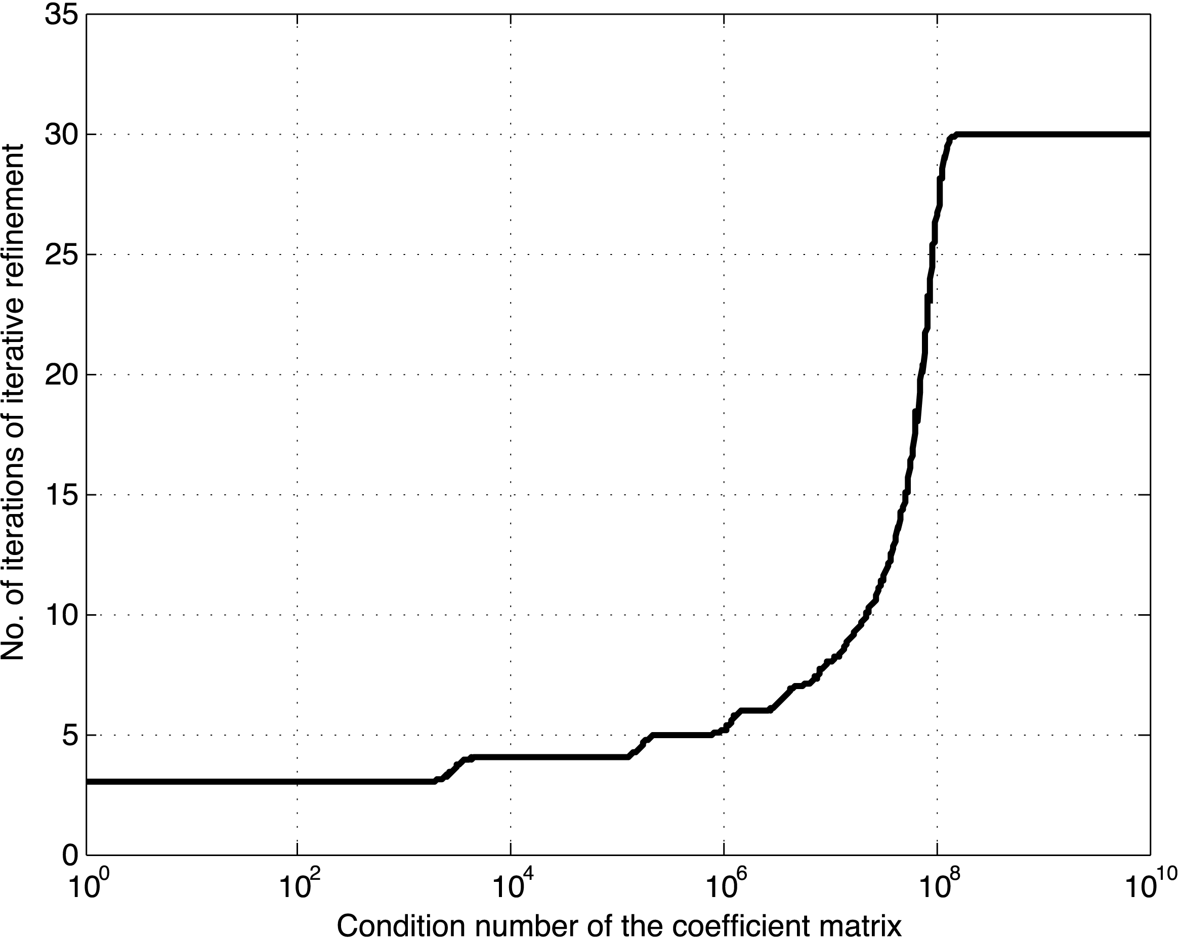
In Figure 9.3, we show the number of iterations needed for our mixed precision method to converge to better accuracy than the associated double precision solve. The number of iterations is shown as a function of the condition number of the coefficient matrix ( ${\it\kappa}$) in the context of a direct dense non-symmetric solve. For each condition number, we have taken 200 random matrices of size
 $200\times 200$ with a prescribed condition number, and we report the mean number of iterations until convergence. The maximum number of iterations allowed was set to 30, so that 30 means failure to converge (as opposed to convergence in 30 iterations). Datta (Reference Datta1995) has conjectured that the number of iterations necessary for convergence was given by
 $$\begin{eqnarray}\lceil \frac{\ln ({\it\varepsilon}_{d})}{\ln ({\it\varepsilon}_{d})+\ln ({\it\kappa})}\rceil ,\end{eqnarray}$$
where  ${\it\varepsilon}_{d}$ is the machine epsilon in double precision.
We can generalize this formula in the context of our mixed precision approach:
 $$\begin{eqnarray}\lceil \frac{\ln ({\it\varepsilon}_{d})}{\ln ({\it\varepsilon}_{s})+\ln ({\it\kappa})}\rceil ,\end{eqnarray}$$
where  ${\it\varepsilon}_{s}$ is the machine epsilon in single precision.
When  ${\it\kappa}{\it\varepsilon}_{s}$ is above 1, the formula is no longer valid. This is characterized in practice by an infinite number of iterations, that is, lack of convergence of the method.
9.4 Extension to quadruple precision
For applications where double precision arithmetic is not sufficient, the mixed precision iterative refinement technique can be extended naturally to quadruple precision. Quadruple precision is almost always implemented in software by a variety of techniques (e.g., through language support, double–double arithmetic, or modelled through general arbitrary precision arithmetic libraries).
To get a BLAS in quadruple precision, one solution is to use language support (e.g. the quadruple precision REAL*16 defined in Fortran), and compile a reference BLAS for REAL*16 values. Although this is a working solution, since the quadruple precision is implemented in software, performance is much slower than the performance of FP32 computations. This results in large speedups reported by the mixed precision iterative refinement solvers. For example, speedups can be between  $10\times$ for a matrix of size 100 or close to
 $100\times$ for a matrix of size
 $1000$ (Baboulin et al. Reference Baboulin, Buttari, Dongarra, Kurzak, Langou, Langou, Luszczek and Tomov2009).
Another common technique is to use double–double arithmetic, where a double–double value  $d$ is represented as the sum of two double precision values, each supplying half of the significant digits of
 $d$. Thus, arithmetic using double–double representations can be reduced to double precision operations, which is hardware-supported, leading to implementations that can be substantially faster than language-supported or the more general arbitrary precision arithmetic techniques. A drawback is that the double–double technique does not implement IEEE quadruple precision.
9.5 Extension to other algorithms
Mixed precision algorithms can easily provide substantial speedup for very little code effort by mainly taking into account existing hardware properties.
We have shown how to derive mixed precision versions of a variety of algorithms for solving general linear systems of equations. In the context of overdetermined least-squares problems, the iterative refinement technique can be applied to the augmented system (where both the solution and the residual are refined, as described in Demmel, Hida, Li and Riedy Reference Demmel, Hida, Li and Riedy2007), to the QR factorization, to the semi-normal equations, or to the normal equations (Björck Reference Björck1996). Iterative refinement can also be applied for eigenvalue computation (Dongarra, Moler and Wilkinson Reference Dongarra, Moler and Wilkinson1983) and for singular value computation (Dongarra Reference Dongarra1983).
Recently, we developed an innovative mixed precision QR for tall-and-skinny matrices (Yamazaki, Tomov, Dong and Dongarra Reference Yamazaki, Tomov, Dong and Dongarra2014) that uses higher precision at critical parts of the algorithm, resulting in increased numerical stability and several times speedup over the standard algorithms (e.g. CGS, MGS, or Householder QR factorizations). In particular, the algorithm starts from a Cholesky QR algorithm, which is known to be fast (expressed as Level 3 BLAS) but numerically unstable, as the computation goes through normal equations. However, computing the normal equations and other critical parts of the algorithm in double–double precision is shown to be stable, while preserving a performance characteristic of Level 3 BLAS operations (Yamazaki, Tomov and Dongarra Reference Yamazaki, Tomov and Dongarra2015).
We hope the work outlined here will encourage scientists to extend this approach to their own applications.
10 Batched operations
Improved data re-use is what drives the design of algorithms to work well on small problems, which, in the end, delivers higher performance. When working on small problems it is possible to improve the re-use, since as the input data gets loaded into fast memory, it can presumably be used many times until completion of the task. Many numerical libraries and applications already use this functionality, but it needs to be further developed. Examples of this trend include the tile algorithms from the area of dense linear algebra (Agullo et al. Reference Agullo, Demmel, Dongarra, Hadri, Kurzak, Langou, Ltaief, Luszczek and Tomov2009a), various register and cache blocking techniques for sparse computations (Im, Yelick and Vuduc Reference Im, Yelick and Vuduc2004), sparse direct multifrontal solvers (Yeralan, Davis and Ranka Reference Yeralan, Davis and Ranka2013), high-order FEM (Dong et al. Reference Dong, Dobrev, Kolev, Rieben, Tomov and Dongarra2014), and numerous applications including astrophysics (Messer, Harris, Parete-Koon and Chertkow Reference Messer, Harris, Parete-Koon, Chertkow, Manninen and Öster2012), hydrodynamics (Dong et al. Reference Dong, Dobrev, Kolev, Rieben, Tomov and Dongarra2014), image processing, and signal processing (Anderson, Sheffield and Keutzer Reference Anderson, Sheffield and Keutzer2012).
The intention of batched routines is to solve a set of independent problems in parallel. When the matrices are large enough to fully load the device with work, there is no need for batched routines: the set of independent problems can be solved in serial as a sequence of problems. Moreover, it is preferred to solve it in serial, and not in batched fashion, to better enforce locality of data and increase cache re-use. However, when matrices are small (e.g. matrices of size less than or equal to  $512$), the amount of work needed to perform the factorization cannot saturate the device (i.e. CPU or GPU), and thus there is a need for batched routines.
The lack of linear algebra software for small problems is especially noticeable for GPUs. The development for CPUs, as pointed out in Sections 10.1 and 10.3, can be done easily using existing software infrastructure. On the other hand, GPUs, due to their throughput-oriented design, are efficient for large data parallel computations, and have therefore often been used in combination with CPUs, where the CPU handles tasks that are small and difficult to parallelize. The need to overcome the challenges of solving small problems on GPUs is also related to the GPU’s energy efficiency, which is often  $4\times$ to
 $5\times$ better than that of multicore CPUs. To take advantage of this energy efficiency, codes ported to GPUs must also exhibit high efficiency. The main goal in this section is to develop GPU algorithms and their implementations on small problems in order to outperform multicore CPUs in raw performance and energy efficiency. In particular, we target the main one-sided factorizations – LU, QR, and Cholesky – for a set of small dense matrices of the same size.
Figure 10.1 gives a schematic view of the batched problem considered. Basic block algorithms, like the ones in LAPACK (Anderson et al. Reference Anderson, Bai, Bischof, Blackford, Demmel, Dongarra, Ducroz, Greenbaum, Hammarling, McKenney and Sorensen1999), factorize a block of columns at step  $i$, denoted by panel
 $P_{i}$, and then apply the transformations accumulated in the panel factorization to the trailing submatrix
 $A_{i}$.
Schematic view of a batched one-sided factorization problem for a set of  $k$ dense matrices.
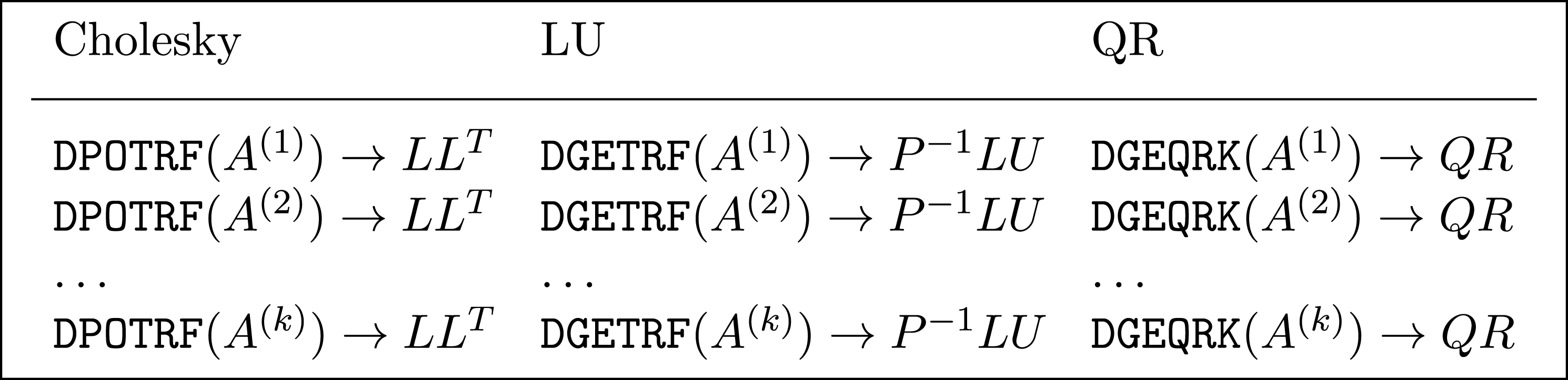
Interleaved with the algorithmic work are questions on what programming and execution model is best for small problems, how to offload work to the GPUs, and what, if any, should be the interaction with the CPUs. The offload-based execution model and the accompanying terms host and device have been established by the directive-based programming standards: OpenACCFootnote 7 and OpenMP 4.0.Footnote 8 While these specifications are host-centric, in the context of dense linear algebra computation, we recognize three distinctly different modes of operation: hybrid, native, and batched execution. The first employs both the host CPU and the device accelerator, whether a GPU or an Intel coprocessor, that cooperatively execute on a particular algorithm. The second offloads the execution to the accelerator completely. The third is the focus of this section, and involves execution of a multitude of small problems on the accelerator while the host CPU only sends the input data and receives the computed result in a pipeline fashion, which alleviates the overheads of limited PCIe bandwidth and comparatively long transfer latency.
10.1 Existing solutions for batched factorizations
Small problems can be solved efficiently on a single CPU core (e.g., using vendor-supplied libraries such as Intel’s Math Kernel LibraryFootnote 9 or AMD’s Core Math LibraryFootnote 10), because the CPU’s memory hierarchy would support ‘natural’ data re-use (sufficiently small problems can fit into small fast memory). Aside from memory re-use, to speed up the computation further, vectorization utilizing SIMD supplementary processor instructions can be added either explicitly, as in Intel’s Pentium III Processor Small Matrix Library,Footnote 11 or implicitly through the vectorization in BLAS. Batched factorizations can then be efficiently computed for multicore CPUs by having a single core factorize a single problem at a time (see Section 10.3). However, as we show, the energy consumption is higher in this scenario than when using the GPU-based factorizations.
For GPU architectures, prior work has concentrated on achieving high performance for large problems through hybrid algorithms (Tomov et al. Reference Tomov, Nath, Ltaief and Dongarra2010b). Motivation came from the fact that the GPU’s computing power cannot be used on panel factorizations as efficiently as on trailing matrix updates (Volkov and Demmel Reference Volkov and Demmel2008). As a result, various hybrid algorithms were developed where panels are factorized on the CPU while the GPU is used for trailing matrix updates (mostly GEMMs: Agullo et al. Reference Agullo, Augonnet, Dongarra, Ltaief, Namyst, Thibault, Tomov, Mei and Hwu2010, Dongarra et al. Reference Dongarra, Haidar, Kurzak, Luszczek, Tomov and Yarkhan2014). For sufficiently large problems, the panel factorizations and associated CPU–GPU data transfers can be overlapped with GPU work. For small problems, however, this is not possible, and our experience has shown that hybrid algorithms would not be as efficient as they are for large problems.
Indeed, targeting very small problems (up to 128), Villa et al. (Villa, Fatica, Gawande and Tumeo Reference Villa, Fatica, Gawande and Tumeo2013a, Villa, Gawande and Tumeo Reference Villa, Gawande and Tumeo2013b) obtained good results for batched LU developed entirely for GPU execution, where a single CUDA thread, or a single thread block, was used to solve one system at a time. Similar techniques, including the use of a single CUDA thread warp for single factorization, were investigated by Wainwright and Sweden (Reference Wainwright and Sweden2013) for LU with full pivoting on matrices of size up to 32. Although the problems considered were often small enough to fit into the GPU’s shared memory (e.g. 48 KB on a K40 GPU) and thus benefit from data re-use ( $n^{2}$ data for
 $\frac{2}{3}n^{3}$ flops for LU), the results showed that the performance in these approaches, up to about 20 Gflops in double precision, did not exceed the maximum performance due to memory-bound limitations (e.g. 46 Gflops on a K40 GPU for DGEMV’s
 $2n^{2}$ flops on
 $n^{2}$ data; see also the performance analysis in Section 10.6.2).
This section introduces a different approach based on batched BLAS, plus some batched-specific algorithmic improvements, that – performance-wise – exceed the memory-bound limitations mentioned above. A batched LU based on batched BLAS was also developed recently and released through cuBLAS,Footnote 12 but this batched LU achieves lower performance compared to our approach when one factors in the algorithmic improvements.
10.2 Algorithmic background
We present a brief overview of the linear algebra aspects for development of either Cholesky, Gauss, or the Householder QR factorizations based on block outer-product updates of the trailing matrix. Conceptually, one-sided factorization maps a matrix  $A$ into a product of matrices
 $X$ and
 $Y$:
 $$\begin{eqnarray}{\mathcal{F}}:\left[\begin{array}{@{}cc@{}}A_{11} & A_{12}\\ A_{21} & A_{22}\\ \end{array}\right]\mapsto \left[\begin{array}{@{}cc@{}}X_{11} & X_{12}\\ X_{21} & X_{22}\\ \end{array}\right]\times \left[\begin{array}{@{}cc@{}}Y_{11} & Y_{12}\\ Y_{21} & Y_{22}\\ \end{array}\right].\end{eqnarray}$$
Algorithmically, this corresponds to a sequence of in-place transformations of  $A$, whose storage is overwritten with the entries of matrices
 $X$ and
 $Y$ (
 $P_{ij}$ indicates currently factorized panels):
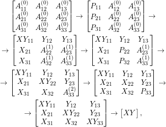 $$\begin{eqnarray}\displaystyle & \left[\begin{array}{@{}ccc@{}}A_{11}^{(0)} & A_{12}^{(0)} & A_{13}^{(0)}\\ A_{21}^{(0)} & A_{22}^{(0)} & A_{23}^{(0)}\\ A_{31}^{(0)} & A_{32}^{(0)} & A_{33}^{(0)}\\ \end{array}\right]\rightarrow \left[\begin{array}{@{}ccc@{}}P_{11} & A_{12}^{(0)} & A_{13}^{(0)}\\ P_{21} & A_{22}^{(0)} & A_{23}^{(0)}\\ P_{31} & A_{32}^{(0)} & A_{33}^{(0)}\\ \end{array}\right]\rightarrow & \displaystyle \nonumber\\ \displaystyle & \rightarrow \left[\begin{array}{@{}ccc@{}}XY_{11} & Y_{12} & Y_{13}\\ X_{21} & A_{22}^{(1)} & A_{23}^{(1)}\\ X_{31} & A_{32}^{(1)} & A_{33}^{(1)}\\ \end{array}\right]\rightarrow \left[\begin{array}{@{}ccc@{}}XY_{11} & Y_{12} & Y_{13}\\ X_{21} & P_{22} & A_{23}^{(1)}\\ X_{31} & P_{32} & A_{33}^{(1)}\\ \end{array}\right]\rightarrow & \displaystyle \nonumber\\ \displaystyle & \rightarrow \displaystyle \left[\begin{array}{@{}ccc@{}}XY_{11} & Y_{12} & Y_{13}\\ X_{21} & XY_{22} & Y_{23}\\ X_{31} & X_{32} & A_{33}^{(2)}\\ \end{array}\right]\rightarrow \left[\begin{array}{@{}ccc@{}}XY_{11} & Y_{12} & Y_{13}\\ X_{21} & X_{22} & Y_{23}\\ X_{31} & X_{32} & P_{33}\\ \end{array}\right]\rightarrow & \displaystyle \nonumber\\ \displaystyle & \rightarrow \left[\begin{array}{@{}ccc@{}}XY_{11} & Y_{12} & Y_{13}\\ X_{21} & XY_{22} & Y_{23}\\ X_{31} & X_{32} & XY_{33}\\ \end{array}\right]\rightarrow \left[\begin{array}{@{}c@{}}XY\end{array}\right], & \displaystyle \nonumber\end{eqnarray}$$
where  $XY_{ij}$ is a compact representation of both
 $X_{ij}$ and
 $Y_{ij}$ in the space originally occupied by
 $A_{ij}$.
There are two distinct phases in each step of the transformation from  $[A]$ to
 $[XY]$: panel factorization (
 $P$) and trailing matrix update
 $A^{(i)}\rightarrow A^{(i+1)}$. Implementation of these two phases leads to a straightforward iterative scheme shown in Algorithm 17.

Algorithm 17 is called a block algorithm since every panel  $P$ is of size
 $nb$, which allows the trailing matrix update to use the Level 3 BLAS routines. Note that if
 $nb=1$, the algorithm falls back to the standard algorithm introduced by LINPACK in the 1980s. The factorization of each panel is accomplished by a non-blocked routine. Table 10.1 shows the BLAS and LAPACK routines that should be substituted for the generic routines named in the algorithm.
Panel factorization and trailing matrix update routines.
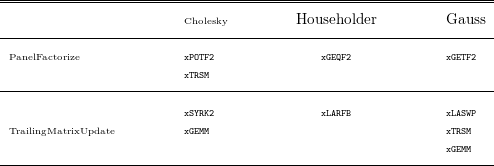
Most of the current libraries focus on large matrices by using hybrid (CPU–GPU) algorithms, e.g. Innovative Computing Lab’s MAGMA.Footnote 13 Because the panel factorization is considered a latency-bound workload, which faces a number of inefficiencies on throughput-oriented GPUs, performing its factorization on the CPU is preferred. Due to their high performance rate exhibited on the update operation, and the fact that the update requires the majority of floating-point operations, the GPU has to perform the trailing matrix update. Note that a data transfer of the panel to and from the CPU is required at each step of the loop. The classical implementation as described in Algorithm 17 lacks efficiency because only either the CPU or the GPU is working at one time. The MAGMA library modified the algorithm further to overcome this issue, and to improve performance. In fact, the ratio of the computational capability between the CPU and the GPU is orders of magnitude, and thus look-ahead is the common technique to alleviate this imbalance and keep the GPU loaded.
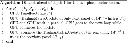
Algorithm 18 shows a very simple case of look-ahead of depth  $1$. The update operation is split into an update of the next panel, and an update of the rest of the trailing matrix. The splitting is done to overlap the communication and the factorization of the panel with the update operation. This technique allows us hide the memory-bound operation of the panel factorization and also keep the GPU loaded by the trailing matrix update.
In the batched implementation, however, we cannot afford such a memory transfer at any step, since the trailing matrix is small and the amount of computation is not sufficient to overlap it in time with the panel factorization. Many small data transfers will take away any performance advantage afforded by the GPU.
10.3 Batched factorizations for multicore CPUs
In broad terms, there are two main ways to approach batched factorization on multicore CPUs. The first approach is to parallelize each small factorization across all the cores, and the second approach is to execute each factorization sequentially on a single core, with all the cores working independently on their own input data. With these two extremes clearly delineated, it is easy to see the third possibility: the in-between solution where each matrix is partitioned among a handful of cores and multiple matrices are worked on at a time as the total number of available cores permits.
The tall-and-skinny matrix factorization scenarios have been studied in the past (Dongarra, Faverge, Ltaief and Luszczek Reference Dongarra, Faverge, Ltaief and Luszczek2012, Luszczek and Dongarra Reference Luszczek and Dongarra2012), which has some relation to batched factorization on multicore CPUs. The problem can be of reduced size, and be fully cache-contained even for Level 1 cache, in which case the algorithm becomes compute-bound because the cache can fully satisfy the issue rate of the floating-point units. However, for our target matrix sizes, the cache containment condition does not hold, and consequently, the most efficient scheme is to employ fixed matrix partitioning schemes with communication based on cache coherency protocols to achieve a nearly linear speedup over a purely sequential implementation (Dongarra et al. Reference Dongarra, Faverge, Ltaief and Luszczek2012, Luszczek and Dongarra Reference Luszczek and Dongarra2012). To our knowledge, this work constitutes a nearly optimal implementation scenario that far exceeds the currently available state-of-the-art vendor and open-source implementations. Unfortunately, the bandwidth still remains the ultimate barrier: the achieved performance could be multiple times better than the next best solution, but it is still a fraction of the peak performance of the processor.
For batched operations, the cache partitioning techniques did not work well in our experience because of the small matrices, which are not the intended target for this kind of optimization. We tested various levels of nested parallelism to exhaust all possibilities of optimization available on CPUs. The two extremes mentioned above get about 40 Gflops (one outer task and all 16 cores working on a single problem at a time; 16-way parallelism for each matrix) and 100 Gflops (16 outer tasks with only a single core per task; sequential execution for each matrix), respectively. The scenarios that fall between these extremes achieve somewhere in between in terms of performance. For example, with eight outer tasks with two cores per task, we achieve about 50 Gflops. Given these results, and to increase clarity of the presentation, we only report the extreme setups in the results shown below.
10.4 Batched factorizations for GPUs
One approach to the batched factorization problem for GPUs is to consider that the matrices are small enough to factor them using the non-blocked algorithm. The implementation in this case is simple, but the performance obtained turns out to be unacceptably low. Thus the implementation of the batched factorization must also be blocked and follow the same iterative scheme (panel factorization and trailing matrix update) shown in Algorithm 17. Note that the trailing matrix update consists of Level 3 BLAS operations (xSYRK for Cholesky, xGEMM for LU and xLARFB for QR) which are compute-intensive and perform very well on the GPU. Thus, the most difficult phase of the algorithm is the panel factorization.
A recommended way of writing efficient GPU kernels is to use the GPU’s shared memory – load it with data and re-use those data in computations as much as possible. The idea behind this is to do the maximum amount of computation before writing the result back to the main memory. However, implementation of such a technique may be complicated for the small problems considered here since it depends on the hardware, the precision, and the algorithm. Moreover, our experience showed that this procedure provides very good performance for simple GPU kernels but it is not that appealing for a batched algorithm, for two main reasons. First, the shared memory is 48 KB per streaming multiprocessor (SMX) for the NVIDIA K40 (Kepler) GPUs, which is a low limit on the size of batched problem data that can fit simultaneously. Second, completely saturating the shared memory per SMX can decrease the performance of memory-bound routines, since only one thread block will be mapped to that SMX at a time. Indeed, due to a limited parallelism in the factorization of a small panel, the number of threads used in the thread block will be limited, resulting in low occupancy, and subsequently poor core utilization. In our study and analysis we found that redesigning the algorithm to use a small amount of shared memory per kernel (less than 10 KB) not only provides an acceptable data re-use but also allows many thread blocks to be executed by the same SMX in parallel, and thus take better advantage of its resources. As a result, the performance obtained is more than  $3\times$ better than when the entire shared memory is used. Since the CUDA warp consists of 32 threads, it is recommended to develop CUDA kernels that use multiples of 32 threads per thread block. For our batched algorithm, we discovered empirically that the best value for
 $nb$ is 32.
Below is a description of batched GPU routines based on batched BLAS kernels. All the relevant optimizations are also discussed. For convenience, we focus only on double precision performance. The methodology and the design ideas remain the same for any precision.
10.4.1 Methodology based on batched BLAS
In a batched problem solution methodology that is based on batched BLAS, there are many small dense matrices that must be factorized simultaneously (as illustrated in Figure 10.1). This means that all the matrices will be processed simultaneously by the same kernel. However, each matrix problem is still solved independently, identified by a unique batch ID. We follow this model in our batched implementations and developed the following set of new batched CUDA kernels.
∙ Cholesky panel. This provides the batched equivalent of LAPACK’s DPOTF2 routine. At step
$j$ of a panel of size $(m,nb)$, the column vector $A(j:m,j)$ must be computed. This requires a dot-product using row $A(j,1:j)$ to update element $A(j,j)$, followed by a DGEMV$A(j+1,1)A(j,1:j)=A(j+1:m,j)$, and finally a DSCAL on column $A(j+1:m,j)$. This routine involves two Level 1 BLAS calls (dot and scal), as well as a Level 2 BLAS DGEMV. Since there are $nb$ steps, these routines are called $nb$ times, and thus one can expect the performance to depend on the performances of Level 2 and Level 1 BLAS operations. Hence, it is a slow, memory-bound algorithm. We used shared memory to load both row $A(j,1:j)$ and column $A(j+1:m,j)$ to re-use them, and wrote a customized batched DGEMV kernel to read and write these vectors from/into the shared memory.∙ LU panel. This provides the batched equivalent of LAPACK’s DGETF2 routine to factorize panels of size
$m\times nb$ at each step of the batched LU factorizations. It consists of three Level 1 BLAS calls (idamax, DSWAP and DSCAL) and one Level 2 BLAS call (DGER). The DGETF2 procedure proceeds as follows. Find the maximum element of the $i$th column, then swap the $i$th row with the row owning the maximum, and scale the $i$th column. To achieve higher performance and minimize the effect on the Level 1 BLAS operation, we implemented a tree reduction to find the maximum pivot where all the threads contribute to find the pivot. Since it is the same column that is used to find the max, then scaled, we load it into the shared memory. These are the only data that we can re-use within one step.∙ QR panel. This provides the batched equivalent of LAPACK’s DGEQR2 routine to perform the Householder panel factorizations. It consists of
$nb$ steps where each step calls a sequence of the DLARFG and the DLARF routines. At every step (to compute one column), the DLARFG involves a norm computation followed by a DSCAL that uses the results of the norm computation in addition to some underflow/overflow checking. The norm computation is a sum reduce and thus a synchronization step. To accelerate it, we implemented a two-layer tree reduction where, for sizes larger than 32, all 32 threads of a warp progress required to do a tree reduction similar to the MPI_REDUCE operation – and the latest 32 element – are reduced by only one thread. Another optimization is to allow more than one thread block to execute the DLARFG kernel, which means that the kernel needs to be split in two – one for norm and one for scaling – in order to guarantee the synchronization. Customized batched implementations of both DLARFG and the DLARF have been developed.∙ Trailing matrix updates. Trailing matrix updates are mainly Level 3 BLAS operations. However, for small matrices, it might be difficult to extract performance from very small Level 3 BLAS kernels. The DGEMM is the best Level 3 BLAS kernel: it is GPU-friendly, highly optimized, and achieves the highest performance among BLAS. Thus, high performance can be achieved if we redesign our update kernels to be represented by DGEMMs. For Cholesky, the update consists of the DSYRK routine. It performs a rank-
$nb$ update on either the lower or upper portion of $A_{22}$. Since cuBLAS does not provide a batched implementation of this routine, we implemented our own. It is based on a sequence of customized DGEMMs in order to extract the best possible performance. The trailing matrix update for Gaussian elimination (LU) is composed of three routines: the DLASWP, which swaps the rows on the left and right of the panel in consideration, followed by the DTRSM to update $A_{12}\leftarrow L_{11}^{-1}A_{12}$, and finally a DGEMM for the update $A_{22}\leftarrow A_{22}-A_{21}L_{11}^{-1}A_{12}$. The swap (or pivoting) is required to improve the numerical stability of Gaussian elimination. However, pivoting can be a performance killer for matrices stored in column-major format because rows in that case are not stored continuously in memory, and thus cannot be read en masse. Indeed, a factorization stored in column-major format can be $2\times$ slower (depending on hardware and problem sizes) than implementations that transpose the matrix in order to use a row-major storage format internally (Volkov and Demmel Reference Volkov and Demmel2008). Nevertheless, experiments showed that this conversion is too expensive for batched problems. Moreover, the swapping operations are serial, that is row by row, which limits the parallelism. To minimize this penalty, we propose a new implementation that emphasizes a parallel swap and allows coalescent read/write. We also developed a batched DTRSM. It loads the small $nb\times nb$$L_{11}$ block into shared memory, inverts it with the DTRTRI routine, and then the $A_{12}$ update is accomplished by a DGEMM. Generally, computing the inverse of a matrix may compromise the numerical stability of the method, but since $A_{11}$ results from numerically stable LU with partial pivoting, and its size is just $nb\times nb$, or in our case $32\times 32$, we do not have this problem (DuCroz, Dongarra and Higham Reference Ducroz, Dongarra and Higham1992). For the Householder QR decomposition the update operation is used by the DLARFB routine. We implemented a batched DLARFB that is composed of three calls to the batched DGEMM: $$\begin{eqnarray}A_{22}\leftarrow (I-VT^{H}V^{H})A_{22}\equiv (I-A_{21}T^{H}A_{21}^{H})A_{22}.\end{eqnarray}$$









10.5 Other techniques for high-performance batched factorizations
10.5.1 Parallel swapping
Profiling the batched LU reveals that more than 60% of the time is spent in the swapping routine. Figure 10.2 shows the execution trace of the batched LU for  $2000$ matrices of size
 $512$. We can observe on the top trace that the classical DLASWP kernel is the most time-consuming part of the algorithm. The swapping consists of
 $nb$ successive interchanges of two rows of the matrices. The main reason that this kernel is the most time-consuming is because the
 $nb$ row interchanges are performed in a sequential order, and the data of a row are not coalescent, thus the thread warps do not read/write it in parallel. It is clear that the main bottleneck here is the memory access. Indeed, slow memory access compared to high computing capability has been a persistent problem for both CPUs and GPUs. CPUs alleviate the effect of long latency operations and bandwidth limitations by using hierarchical caches.
Execution trace of the batched LU factorization using either classical swap (a) or our new parallel swap (b).
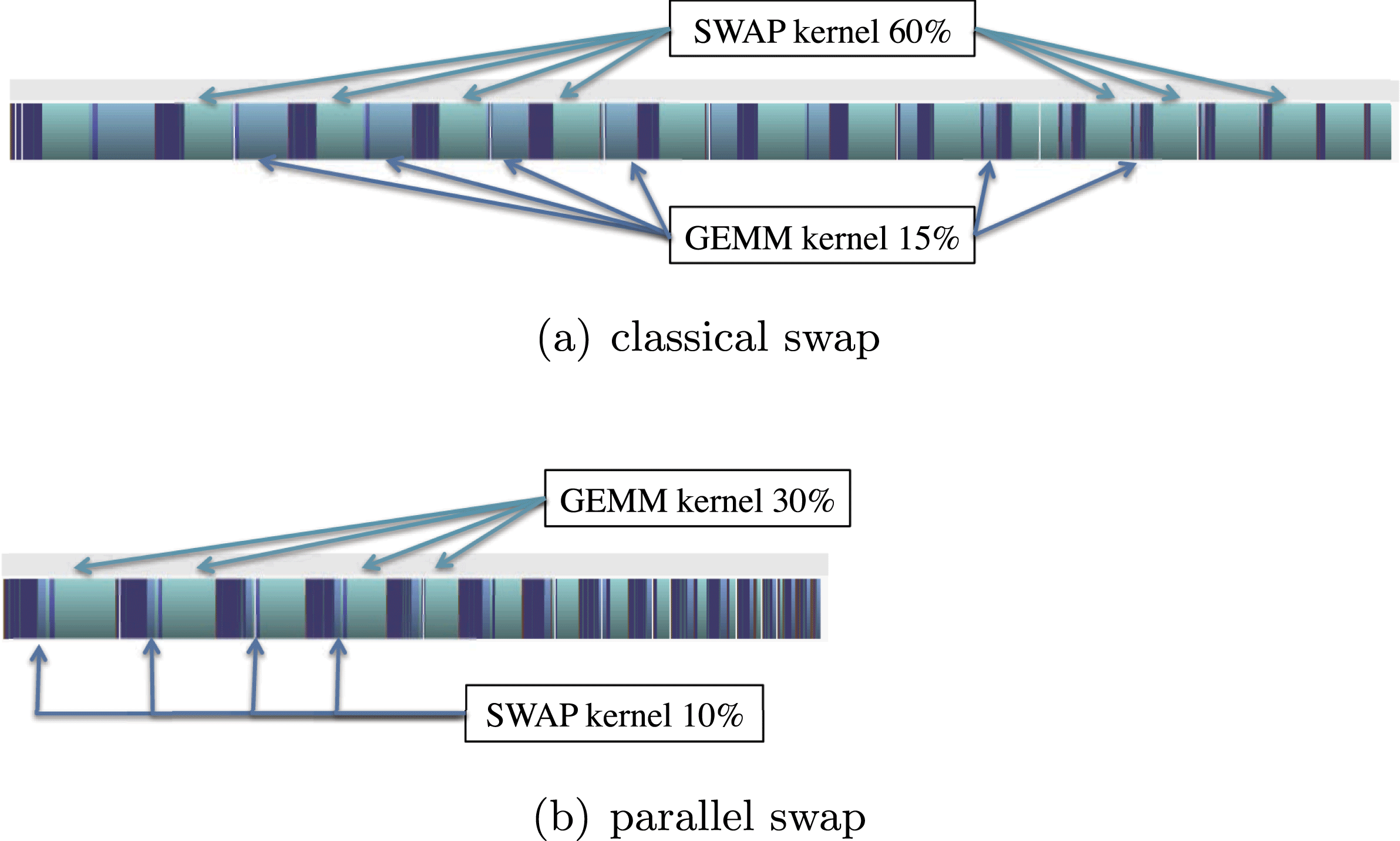
Accelerators, on the other hand, in addition to hierarchical memories, use thread level parallelism (TLP), where threads are grouped into warps and multiple warps are assigned for execution on the same SMX unit. The idea is that when a warp issues an access to the device memory, it stalls until the memory returns a value, while the accelerator’s scheduler switches to another warp. In this way, even if some warps stall, others can execute, keeping functional units busy while resolving data dependencies, branch penalties, and long latency memory requests. In order to overcome the bottleneck of swapping, we propose to modify the kernel to apply all  $nb$ row swaps in parallel. This modification will also allow the coalescent write back of the top
 $nb$ rows of the matrix. Note that the first
 $nb$ rows are those used by the DTRSM kernel that is applied right after the DLASWP, so one optimization is to use shared memory to load a chunk of the
 $nb$ rows, and apply the DLASWP followed by the DTRSM. We changed the algorithm to generate two pivot vectors. The first vector stores the indices of the final destination (e.g. row indices) of the top
 $nb$ rows of the panel. The second stores the row indices of the
 $nb$ rows to swap out and bring into the top
 $nb$ rows of the panel. Figure 10.2 depicts the execution trace (bottom) when using our parallel DLASWP kernel. The experiment shows that this reduces the time spent in the kernel from 60% to around 10% of the total elapsed time. Note that the colours between the top and the bottom traces do not match each other; this is because the NVIDIA profiler automatically chooses the tracing colour. As a result, the performance gain obtained is about
 $1.8\times$ as shown in Figure 10.3. We report each of the proposed optimizations for the LU factorization in Figure 10.3, but we would like to mention that the percentage of improvement obtained for the Cholesky and QR factorization is similar, and to simplify we reported the LU factorization only. Note that starting from this version we were able to be faster than the cuBLAS implementation of the batched LU factorization.
Performance in Gflops of the different versions of our batched LU factorizations compared to the cuBLAS implementation for different matrix sizes, where  $m=n$.
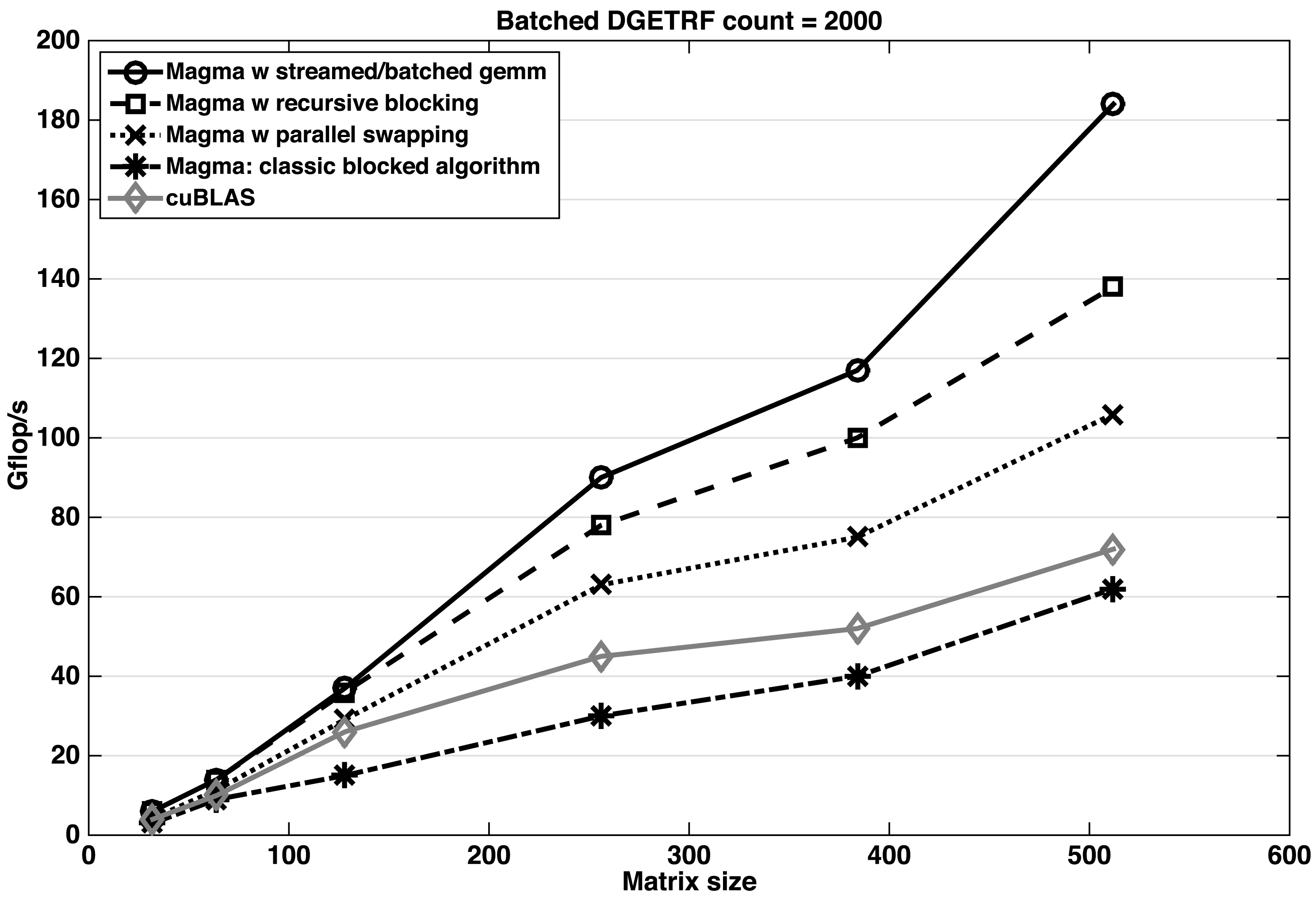
10.5.2 Recursive nested blocking
The panel factorizations described in Section 10.4.1 factorize the  $nb$ columns one after another, similarly to the LAPACK algorithm. At each of the
 $nb$ steps, either a rank-one update is required to update the vectors to the right of the factorized column
 $i$ (this operation is done by the DGER kernel for LU and the DLARF kernel for QR), or a left-looking update of column
 $i$ by the columns on its left is required, before factorizing it (this operation is done by DGEMV for the Cholesky factorization). Since we cannot load the entire panel into the shared memory of the GPU, the columns to the right (in the cases of LU and QR) or to the left (in the case of Cholesky) are loaded back and forth from the main memory at every step. Thus, one can expect that this is the most time-consuming part of the panel factorization. A detailed analysis using the profiler reveals that the DGER kernel requires more than
 $80$% of the panel time and around
 $40$% of the total LU factorization time. Similarly for the QR decomposition, the DLARF kernel used inside the panel computation needs
 $65$% of the panel time and
 $33$% of the total QR factorization time. Likewise, the DGEMV kernel used within the Cholesky panel computation needs around
 $91$% of the panel time and
 $30$% of the total Cholesky factorization time. These routines’ inefficient behaviour is also due to the memory access. To overcome that bottleneck, we propose to improve the efficiency of the panel and to reduce the memory access by using a recursive level of blocking technique: see Figures 10.4 and 10.5. In principle, the panel can be blocked recursively until it is a single element. However, in practice,
 $2$–
 $3$ blocked levels are sufficient to achieve high performance. The above routines must be optimized for each blocked level, which complicates the implementation. More than a
 $30$% boost in performance is obtained with this optimization, as demonstrated in Figure 10.3 for the LU factorization. The same trend has been observed for both the Cholesky and the QR factorization.
Recursive nested blocking.
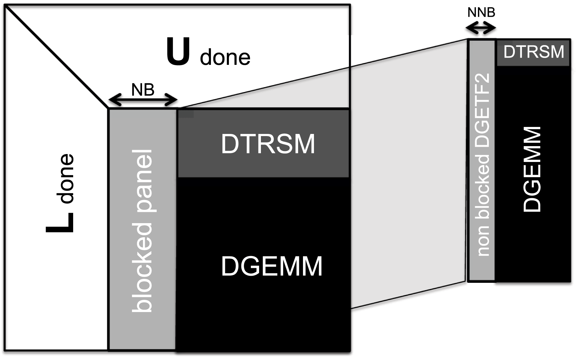
Execution trace of the batched LU factorization using either classical GETF2 (a) or our recursive GETF2 (b).
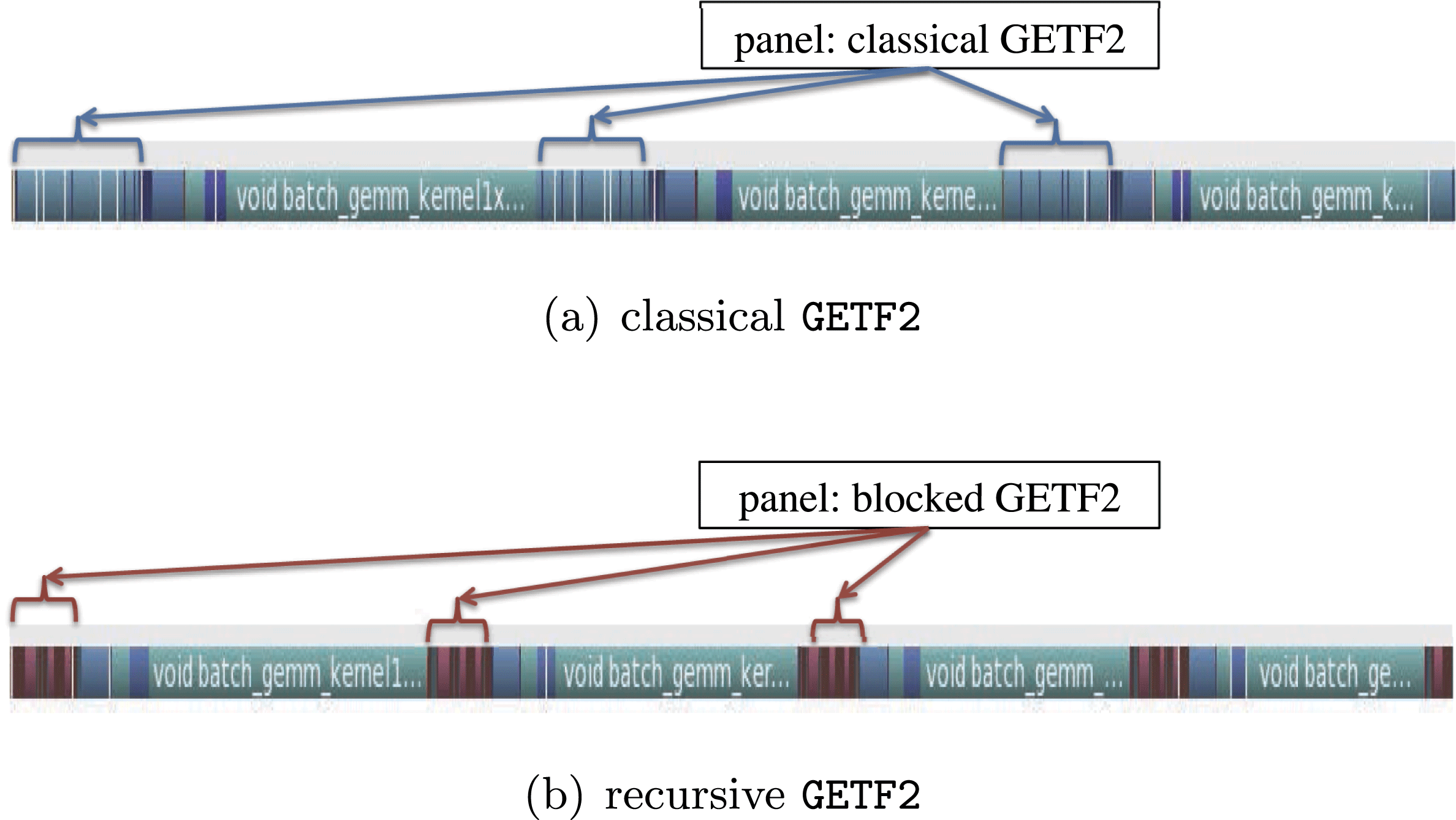
10.5.3 Trading extra computation for higher performance
The challenge discussed here is as follows. For batched problems there is a need to minimize the use of low-performance kernels on the GPU even if they are Level 3 BLAS. For the Cholesky factorization, this concerns the DSYRK routine that is used to update the trailing matrix. The performance of DSYRK is important to the overall performance, since it takes a big part of the runtime. We implemented the batched DSYRK routine as a sequence of DGEMM routines, each of size  $M=m,N=K=nb$. In order to exclusively utilize the DGEMM kernel, our implementation writes both the lower and the upper portion of the
 $nb\times nb$ diagonal blocks of the trailing matrix. This results in
 $nb^{3}$ extra operations for the diagonal block. However, since
 $nb$ is small (e.g.
 $nb=32$), these extra operations can be considered free. In practice the extra operation allows us to use DGEMM and thus achieve higher performance than the one that touches the lower/upper portion of the
 $nb\times nb$ diagonal blocks. Tests show that our implementation of DSYRK is
 $2\times$ faster than the DGEMM kernel for the same matrix size. This shows that our DSYRK is very well optimized for it to reach the performance of DGEMM (which is
 $2\times$ slower since it computes twice as many flops).
We applied the same technique in the DLARFB routine used by the QR decomposition. The QR trailing matrix update uses the DLARFB routine to perform
 $$\begin{eqnarray}A_{22}=(I-VT^{H}V^{H})A_{22}=(I-A_{21}T^{H}A_{21}^{H})A_{22}.\end{eqnarray}$$
The upper triangle of  $V$ is zero with ones on the diagonal.
 $A_{21}$, which stores
 $V$ in its lower triangular part and
 $R$ (part of the upper
 $A$) in its upper triangular part, is available in the classical DLARFB. Therefore, the above is computed using DTRMM for the upper part of
 $A_{21}$ and DGEMM for the lower part. Also, the
 $T$ matrix is an upper triangular and therefore the classical DLARFB implementation uses DTRMM to perform the multiplication with
 $T$. Thus, if one can guarantee that the lower portion of
 $T$ is filled with zeros and the upper portion of
 $V$ is filled zeros and ones on the diagonal, the DTRMM can be replaced by DGEMM. With that in mind, we implemented a batched DLARFB that uses three DGEMM kernels by initializing the lower portion of
 $T$ with zeros, and filling up the upper portion of
 $V$ with zeros and ones on the diagonal. Note that this brings
 $3nb^{3}$ extra operations, but again, the overall time spent in the new DLARFB update using the extra computation is around 10% less than
DTRMM.
Similarly to DSYRK and DLARFB, we implemented the batched DTRSM (that solves  $AX=B$) by inverting the small
 $nb\times nb$ block
 $A$ and using DGEMM to get the final result
 $X=A^{-1}B$.
10.5.4 Block recursive DLARFT algorithm
The DLARFT is used to compute the upper triangular matrix  $T$ that is needed by the QR factorization in order to update either the trailing matrix or the right-hand side of the recursive portion of the QR panel. The classical LAPACK approach computes
 $T$ column by column in a loop over the
 $nb$ columns as described in Algorithm 19. Such an implementation takes up to
 $50$% of the total QR factorization time. This is due to the fact that the kernels needed – DGEMV and DTRMV – require implementations where threads go through the matrix in different directions (horizontal versus vertical, respectively). An analysis of the mathematical formula of computing
 $T$ allowed us to redesign the algorithm to use Level 3 BLAS and to increase the data re-use by putting the column of
 $T$ in shared memory. One can observe that the loop can be split into two loops – one for DGEMV and one for DTRMV. The DGEMV loop that computes each column of
 $\widehat{T}$ can be replaced with one DGEMM to compute all the columns of
 $\widehat{T}$ if the triangular upper portion of
 $A$ is zero and the diagonal is made of ones. This is already needed for our implementation’s trailing matrix update in order to use DGEMM in the DLARFB, and thus can be exploited here as well. For the DTRMV phase, we load the
 $T$ matrix into shared memory as this allows all threads to read/write from/into shared memory during the
 $nb$ steps of the loop. The redesign of this routine is depicted in Algorithm 20. Since we developed a recursive blocking algorithm, we have to compute the
 $T$ matrix for every level of the recursion. Nevertheless, the analysis of Algorithm 20 lets us conclude that the portion of the
 $T$s computed in the lower recursion level is the same as the diagonal blocks of the
 $T$ of the upper level (white triangular blocks in Figure 10.6), and thus we can avoid their (re-)computation. For that, we modified Algorithm 20 in order to compute either the whole
 $T$ or the upper rectangular portion that is missed (dark/pale grey portions in Figure 10.6).
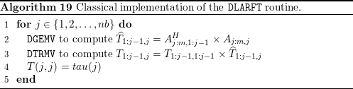

The shape of the matrix  $T$ for different levels of the recursion during the QR decomposition.
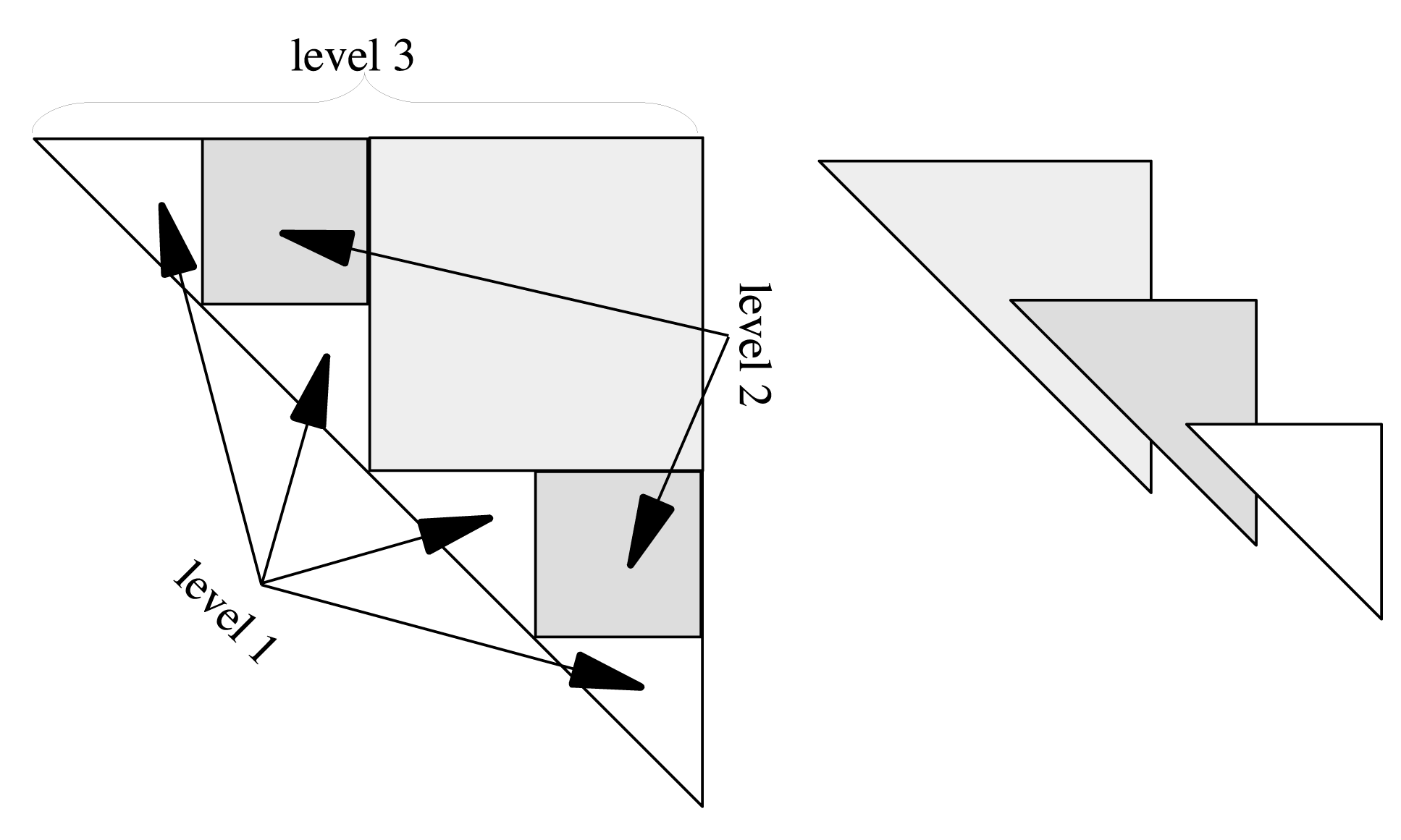
10.5.5 Streamed DGEMM
As our main goal is to achieve higher performance, we performed deep analysis of every kernel of the algorithm. We discovered that  $70$% of the time is spent in the batched DGEMM kernel after the previously described optimizations were applied. An evaluation of the performance of the DGEMM kernel, using either batched or streamed DGEMM, is illustrated in Figure 10.7. The curves let us conclude that the streamed DGEMM is performing better than the batched one for some cases (e.g. for
 $k=32$ when the matrix size is of order
 $m>200$ and
 $n>200$). We note that the performance of the batched DGEMM is stable and does not depend on
 $k$, in the sense that the difference in performance between
 $k=32$ and
 $k=128$ is minor. However, it is bound by 300 Gflops. For that we propose to use the streamed DGEMM whenever it is faster, and to roll back to the batched one otherwise. Figure 10.8 shows the trace of the batched LU factorization of
 $2000$ matrices of size
 $512$ using either the batched DGEMM (top trace) or the combined streamed/batched DGEMM (bottom trace). We can see that the use of the streamed DGEMM (when the size allows it) can speed up the factorization by about
 $20$%.
Performance comparison between streamed and batched DGEMM kernels for different  $K$ and different matrix sizes when
 $m=n$.
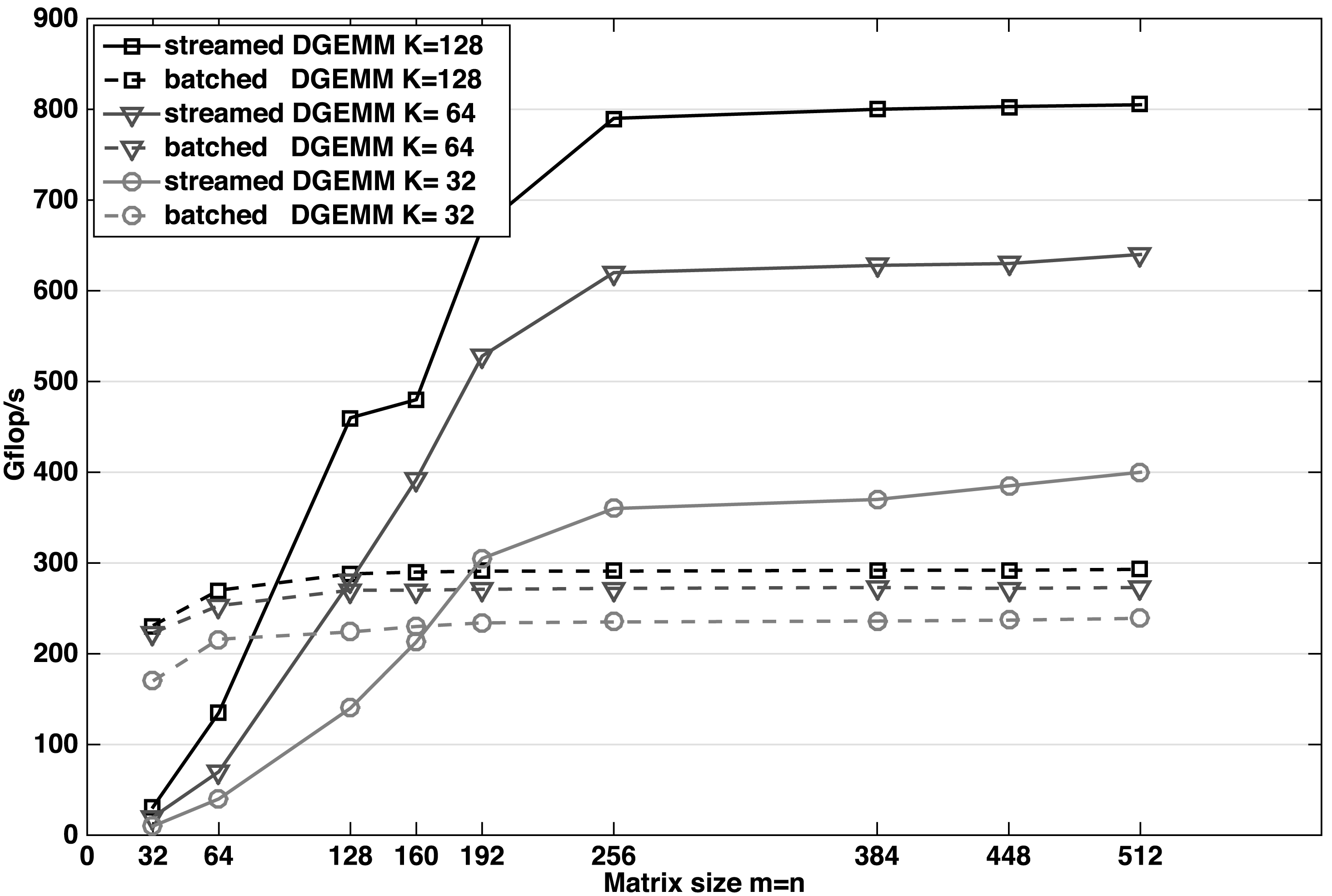
Execution trace of the batched LU factorization using either batched DGEMM (a) or streamed/batched DGEMM (b).
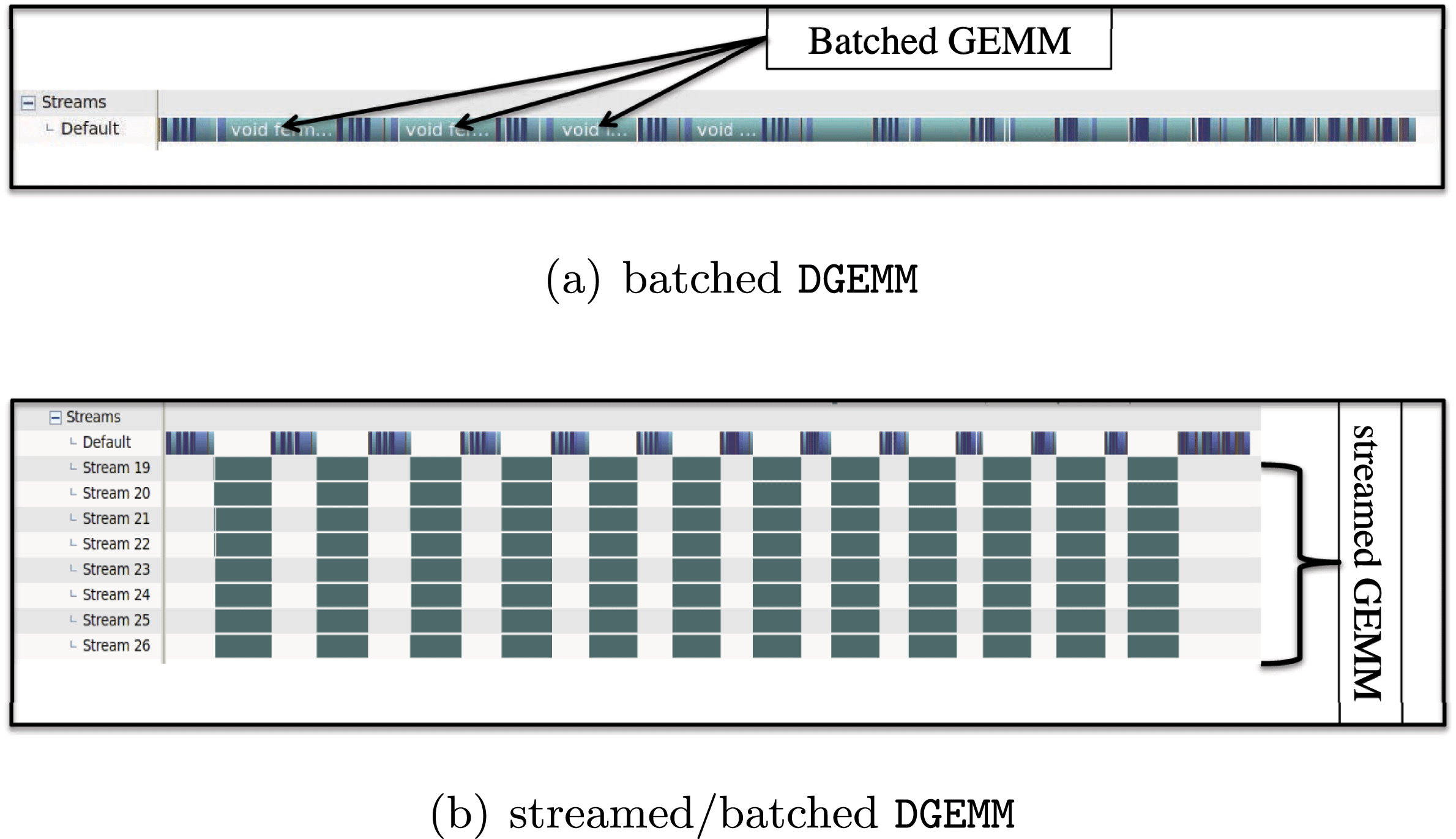
10.6 Performance results
10.6.1 Hardware description and setup
We conducted our experiments on a system with two sockets of 8-core Intel Xeon E5-2670 (Sandy Bridge) processors, each running at 2.6 GHz. Each socket had 20 MB of shared L3 cache, and each core had a private 256 KB L2 and 64 KB L1 cache. The system is equipped with 52 GB of memory and the theoretical peak in double precision is 20.8 Gflops per core, (i.e. 332.8 Gflops in total for the two sockets). It is also equipped with NVIDIA K40c GPUs with  $11.6$ GB of GDDR memory per card, running at
 $825$ MHz. The theoretical peak in double precision is 1689.6 Gflops. The cards are connected to the host via two PCIe I/O hubs with 6 GB/s bandwidth.
A number of software packages were used for the experiments. On the CPU side, we used Intel’s MKL (Math Kernel Library) with the ICC compiler (version 2013.sp1.2.144), and on the GPU accelerators we used CUDA version 6.0.37.
Regarding energy, we note that in this particular setup the CPU and the GPU have about the same theoretical power draw. In particular, the Thermal Design Power (TDP) of the Intel Sandy Bridge is 115 W per socket, or 230 W in total, while the TDP of the K40c GPU is 235 W. Therefore we expect that a GPU would have a rough power consumption advantage if it outperforms (in terms of time to solution) the 16 Sandy Bridge cores. Note that, based on the theoretical peaks, the GPU’s advantage should be about  $4\times$ to
 $5\times$. This is observed in practice as well, especially for regular workloads on large data-parallel problems that can be efficiently implemented for GPUs.
10.6.2 Performance analysis
The performance of the non-blocked versions can be bounded by the performance of the rank-one update. Its flops/bytes ratio for double precision is  $3n/(16+16n)$ (for
 $m=n$). Therefore, a top performance for
 $n=500$ and read/write achievable bandwidth of 160 Gflops would be
 $160\times (3\times 500)/(16+16\times 500)=29.9$ Gflops. This shows for example that our non-blocking LU from Figure 10.3 achieves this theoretically best performance. This is the limit for the other non-blocking one-sided factorizations as well.
A similar analysis for a best expected performance can also be done for the block algorithms. Their upper performances are bounded in general by the rank- $nb$ performance (e.g., illustrated in Figure 10.7 for
 $nb=32$ and
 $64$). As can be seen, we do not reach the asymptotic performance of 400 Gflops even at
 $n=500$. However, the performance grows steadily with
 $n$, which indicates that the operations contributing
 $O(n^{2})$ flops are too slow to saturate the computational capacity of the hardware. The rank-
 $nb$ update, which contributes
 $O(n^{3})$ flops, is thus overshadowed by the
 $O(n^{2})$ contribution. If, however, we let
 $n$ grow further, the rank-
 $nb$ update will eventually dominate the influence of the
 $O(n^{2})$ part.
10.6.3 Comparison with cuBLAS on a K40c
Achieving high performance across accelerators remains a challenging problem that we address with the algorithmic and programming techniques described in this section. The efficient strategies we use exploit parallelism and increase the use of Level 3 BLAS operations across the GPU. We highlighted this through a set of experiments that we performed on our system. We compare our batched implementations with the cuBLAS libraryFootnote 14 whenever possible (cuBLAS features only a DGETRFBatched routine). Our experiments were performed on batches of  $2000$ matrices of different sizes going from
 $32\times 32$ to
 $512\times 512$.
Figure 10.9 shows the performance of LU. The DGETRFBatched version, labelled ‘cuBLAS’, reaches a performance of around 70 Gflops for matrices of size  $512\times 512$. We first compare to a naive implementation that is based on the assumption that matrices of size
 ${<}512$ are very small for block algorithms and therefore uses the non-blocked version. For example, for the case of LU this is the DGETF2 routine. The routine is very slow and the performance obtained reaches less than 30 Gflops, as shown in Figure 10.3. Note that although low, this is also the optimal performance achievable by this type of algorithm, as explained in Section 10.6.2.
Performance in Gflops of our different versions of the batched LU factorization compared to the cuBLAS implementation for different matrix sizes where  $m=n$.
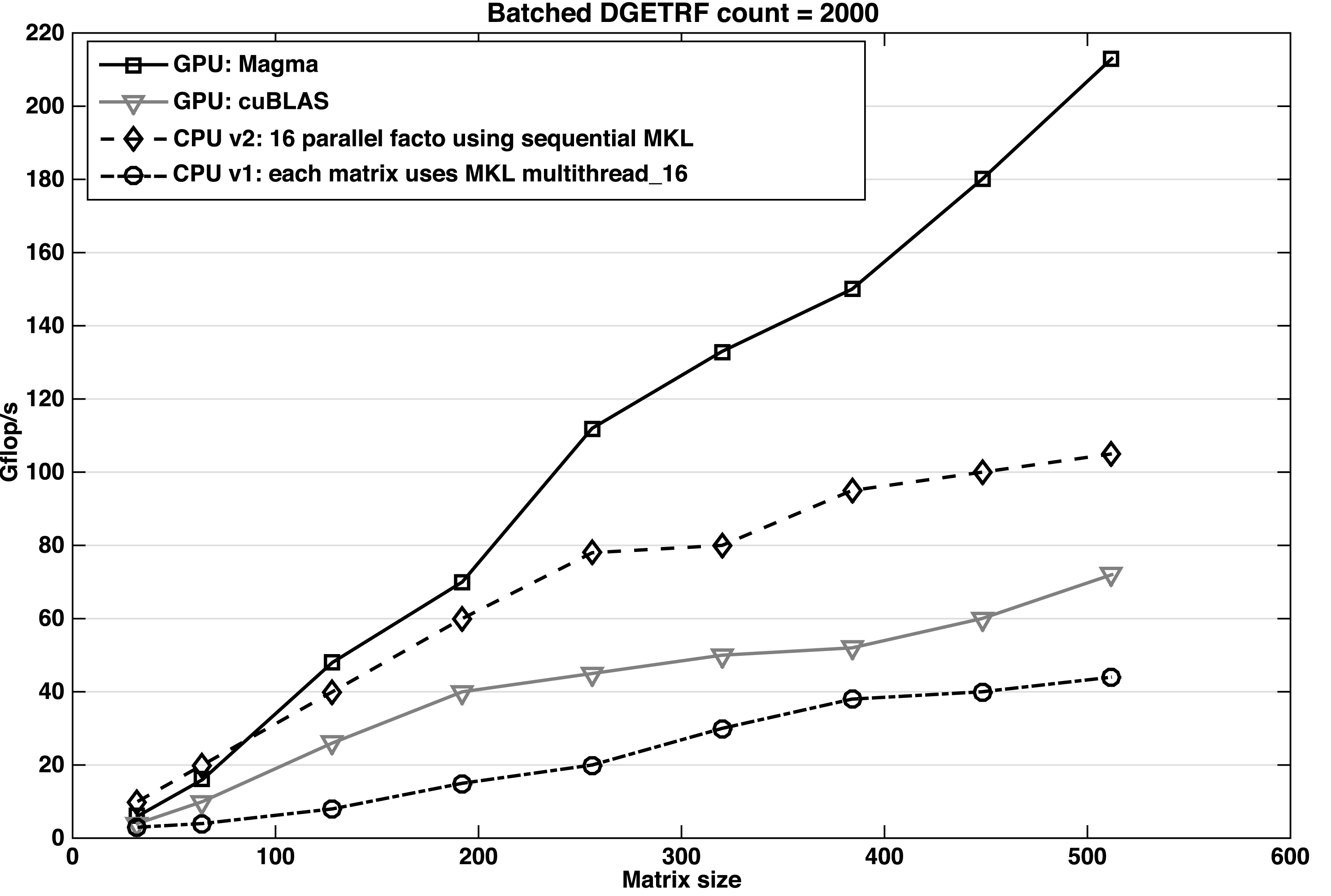
Our second comparison is to the classic LU factorization (i.e., the one that follows LAPACK’s two-phase implementation described in Algorithm 17). This algorithm achieves 63 Gflops as shown in Figure 10.3.
To reach beyond 100 Gflops we used the technique that optimizes pivoting with parallel swap. The next step in performance improvement was the use of two-level blocking of the panel, which enables performance levels that go slightly above 130 Gflops. The last two improvements are streamed/batched GEMM, which moves the performance beyond 160 Gflops, and finally the two-level blocking update (also called recursive blocking), which completes the set of optimizations and takes the performance beyond 180 Gflops. Thus our batched LU achieves up to  $2.5\times$ speedup compared to its counterpart from the cuBLAS library.
10.6.4 Comparison to multicore CPU solutions
Here we compare our batched LU to the two CPU implementations proposed in Section 10.3. The simple CPU implementation is to go in a loop style to factorize matrix after matrix, where each factorization is using the multithread version of the MKL library. This implementation is limited in terms of performance and does not achieve more than 50 Gflops. The main reason for this low performance is the fact that the matrix is small – it does not exhibit parallelism and so the multithreaded code is not able to feed all  $16$ active threads with work. For that we proposed another version of the CPU implementation. Since the matrices are small (
 ${<}512$) and at least
 $16$ of them fit into the L3 cache, one of the best techniques is to use each thread to independently factorize a matrix. In this way
 $16$ factorizations are conducted independently, in parallel. We think that this implementation is one of the best optimized implementations for the CPU. This later implementation is
 $2\times$ faster than the simple implementation, and it reaches around 100 Gflops in factorizing
 $2000$ matrices of size
 $512\times 512$. Experiments show that our GPU batched LU factorization is able to achieve a speedup of
 $1.8\times$ versus the best CPU implementation using
 $16$ Sandy Bridge cores, and
 $4\times$ versus the simple one.
Performance of the GPU versus CPU versions of our batched Cholesky factorizations for different matrix sizes, where  $m=n$.
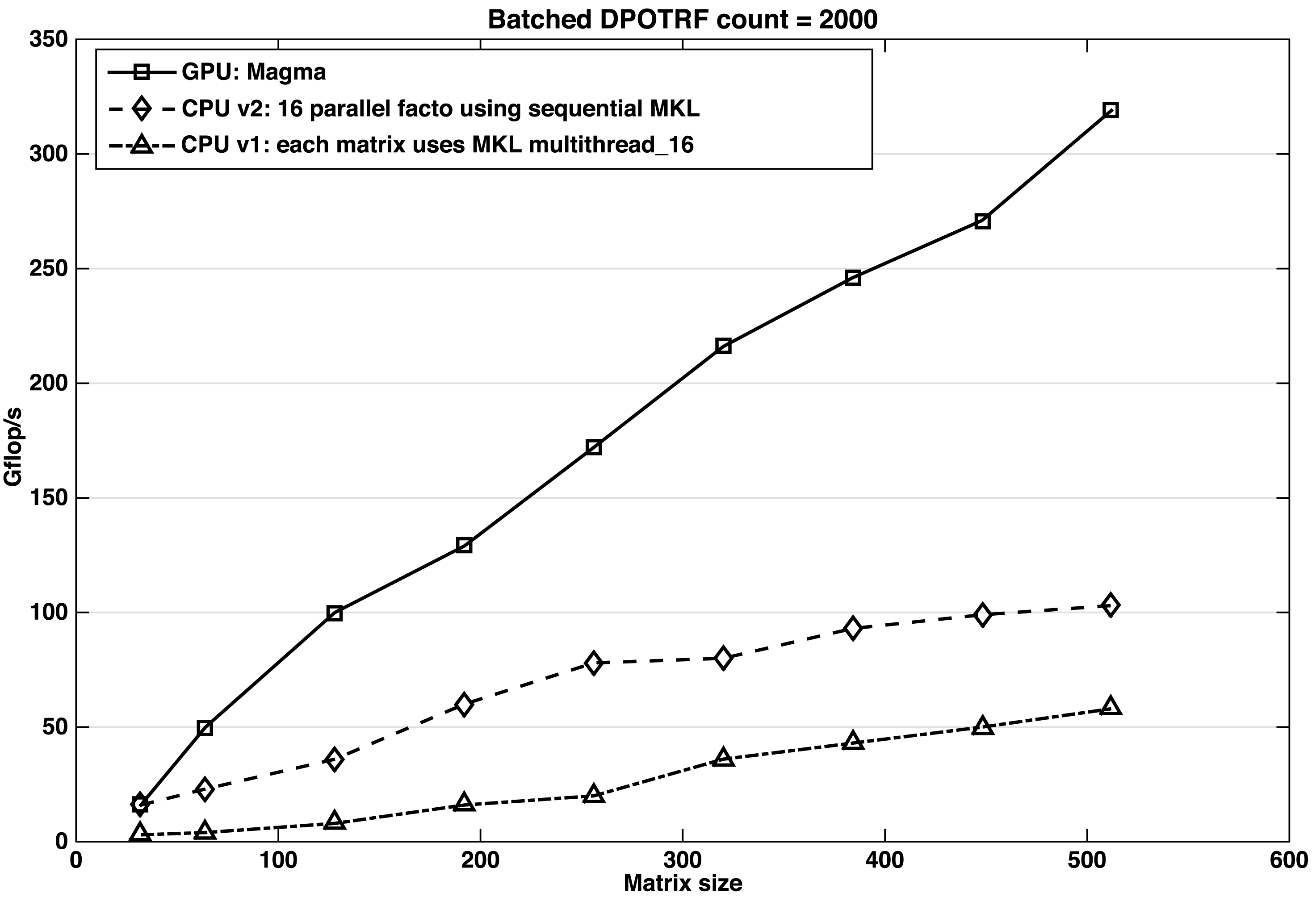
The performance obtained for the Cholesky and QR factorizations are similar to the results for LU. A comparison with the two CPU implementations for Cholesky and QR are given in Figures 10.10 and 10.11, respectively.
Performance of the GPU versus CPU versions of our batched QR decomposition for different matrix sizes, where  $m=n$.
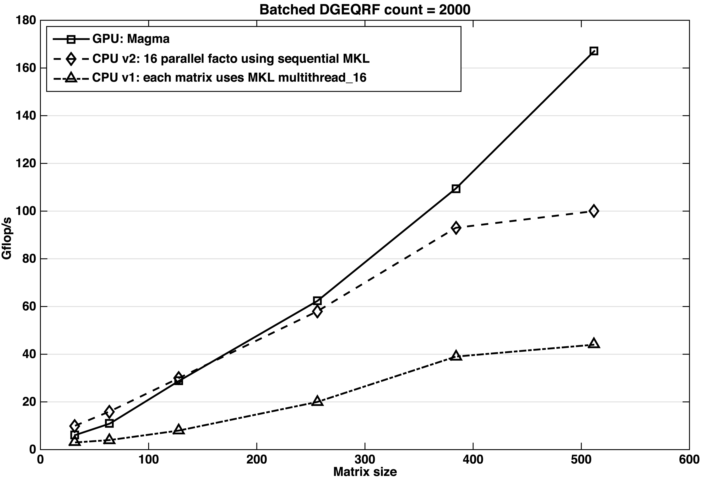
As for the LU, our first GPU implementation of the batched Cholesky factorization follows the classical LAPACK implementation. Compared to the non-blocking algorithm this version increases the use of shared memory and attains, at  $n=500$, an upper bound of 60 Gflops. The different optimization techniques from Section 10.5 drive the performance of the Cholesky factorization up to 200 Gflops. The two CPU implementations behave similarly to those for LU. The simple CPU implementation achieves around 60 Gflops while the optimized one reaches 100 Gflops. This yields a speedup of
 $2\times$ against the best CPU implementation using 16 Sandy Bridge cores.
The progress of our batched QR implementation over the different optimizations shows the same behaviour. The classical block implementation does not attain more than 50 Gflops. The recursive blocking improves performance up to 105 Gflops, and the optimized computation of  $T$ draws it up to 127 Gflops. The other optimizations (replacing DTRMM with DGEMM in both DLARFT and DLARFB), combined with the streamed/batched DGEMM, bring the GPU implementation to around 167 Gflops. The simple CPU implementation of the QR decomposition does not attain more than 50 Gflops while the optimized one gets 100 Gflops. Despite the CPU’s hierarchical memory advantage, our GPU batched implementation is about
 $1.7\times$ faster.
10.6.5 Energy efficiency
For our energy efficiency measurements we use power and energy estimators built into the modern hardware platforms. In particular, on the CPU tested, the Intel Xeon E5-2690, we use RAPL (runtime average power limiting) hardware counters (Intel 2014, Rotem et al. Reference Rotem, Naveh, Rajwan, Ananthakrishnan and Weissmann2012). By the vendor’s own admission, the reported power/energy numbers are based on a model which is tuned to match the actual measurements for various workloads. Given this caveat, we can report that the tested Sandy Bridge CPU on idle, running at a fixed frequency of 2600 MHz, consumes about 20 W of power per socket. Batched operations raise the consumption to above 125–140 W per socket, and the large dense matrix operations, which attain the highest fraction of peak performance, raise the power draw to about 160 W per socket.
For the GPU measurements we use the NVIDIA Management Library (NVML).Footnote 15 NVML provides a C-based program interface for monitoring and managing various states within NVIDIA Tesla GPUs. On Fermi and Kepler GPUs (like the K40c used here) the readings are reported to be accurate to within +/ $-5$% of current power draw. The idle state of the K40c GPU consumes about 20 W. Batched factorizations raise the consumption to about 150–180 W, while large dense matrix operations raise the power draw to about 200 W.
Figure 10.12 depicts a comparison of the power consumption required by the three implementations of the batched QR decomposition: the best GPU and the two CPU implementations. The problem solved here is about  $4000$ matrices of size
 $512\times 512$ each. The dashed curve shows the power required by the simple CPU implementation. In this case the batched QR proceeds as a loop over the
 $4000$ matrices, where each matrix is factorized using the multithreaded DGEQRF routine from the Intel MKL library on the 16 Sandy Bridge cores. The dot-dashed curve shows the power required by the optimized CPU implementation. Here, the code proceeds by a sweep of 16 parallel factorizations, each using the sequential DGEQRF routine from the Intel MKL library. The solid curve shows the power consumption of our GPU implementation of the batched QR decomposition. One can observe that the GPU implementation is attractive because it is around
 $2\times$ faster than the optimized CPU implementation, and moreover, because it consumes
 $3\times$ less energy.
Comparison of the power consumption for the QR decomposition of  $4000$ matrices of size
 $512\times 512$.
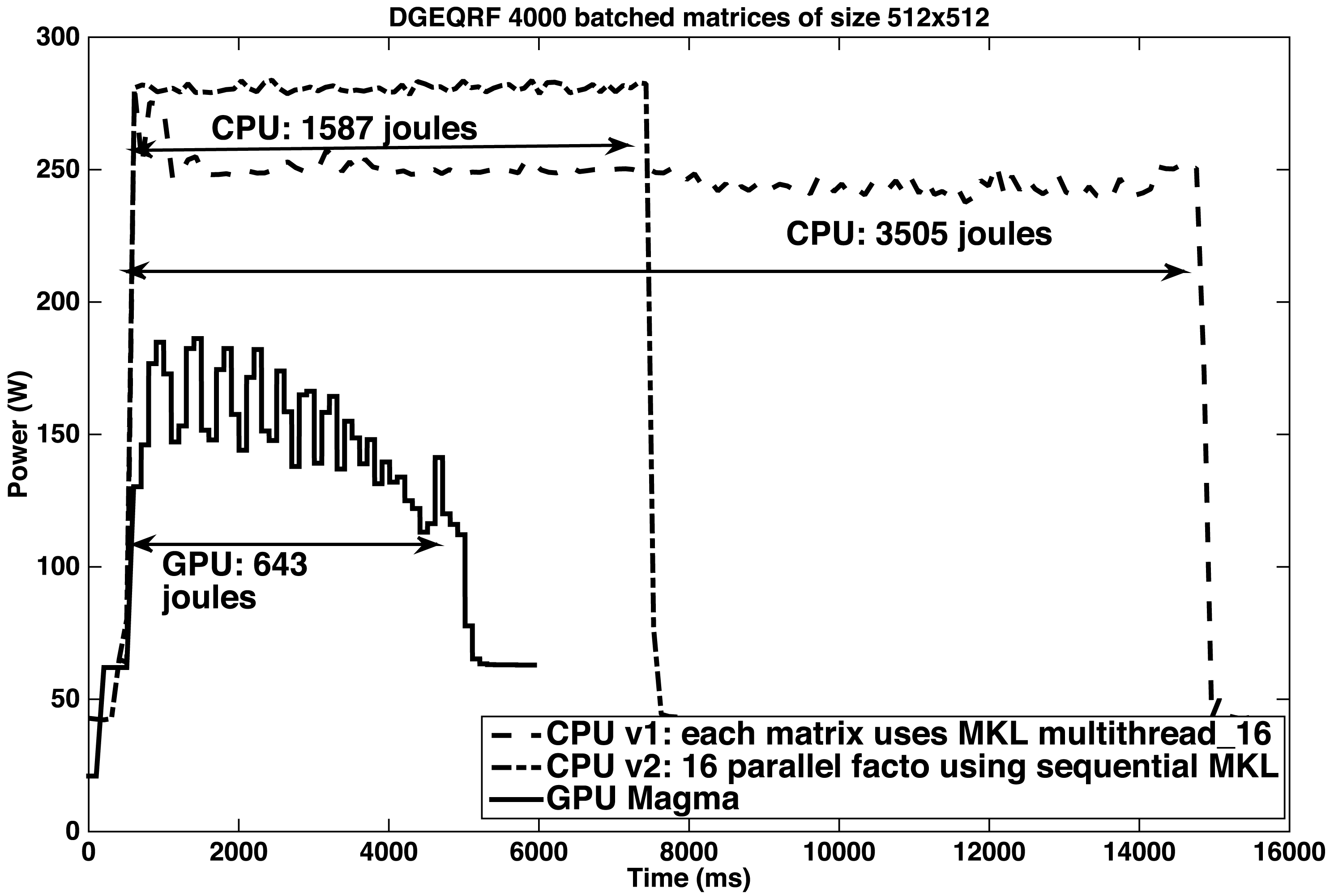
According to our experiments, we found that the GPU implementations of all of the batched one-sided factorizations reach around  $2\times$ speedup over their best CPU counterpart and are
 $3\times$ less expensive in terms of energy.
10.7 Future directions
As the development of efficient small problem solvers becomes more intricate on new architectures, we envision that users will further demand their availability in high-performance numerical libraries, and that batched solvers will actually become a standard feature in those libraries for new architectures. Our plans are to release and maintain this new functionality through the MAGMA libraries for NVIDIA GPU accelerators, Intel Xeon Phi coprocessors, and OpenCL with optimizations for AMD GPUs.
The batched algorithms and techniques can be used and extended to develop GPU-only implementations for stand-alone linear algebra problems. These would be useful, for example, to replace the hybrid CPU–GPU algorithms in cases where energy consumption, instead of higher-performance through use of all available hardware resources, is the top priority. Moreover, GPU-only implementations can have a performance advantage as well, when the host CPU becomes slower compared to the accelerator in future systems. For example, in mobile devices featuring ARM processors enhanced with GPUs, like the Jetson TK1, we have already observed that the GPU-only implementations have a significant advantage in both energy consumption and performance. This has motivated another future work direction – the development and release of a MAGMA Embedded library that would incorporate entirely GPU/coprocessor implementations for stand-alone applications, as well as batched, dense linear algebra problems.
11 Sparse linear algebra
11.1 Approximate ILU preconditioning
Matrix factorizations also play an important role in sparse linear algebra, but in a slightly modified form than for dense systems. For matrices where most entries are zero, it is efficient to explicitly store only the non-zero elements using data layouts specifically designed for these cases (Barrett et al. Reference Barrett, Berry, Chan, Demmel, Donato, Dongarra, Eijkhout, Pozo, Romine and van der Vorst1994a). In this way, only the non-zero entries are considered in the arithmetic computations, while all other entries are implicitly assumed to be zero. If an LU factorization is computed for a (non-singular) sparse matrix, the factors can be much less sparse than the original matrix. Although there exist matrix reordering techniques such as reverse Cuthill–McKee ordering (RCM: Cuthill and McKee Reference Cuthill and Mckee1969) that aim at reduced fill-in, the memory requirements for storing the LU factors can become a bottleneck. With more non-zero entries, the computational cost of the factorization and the forward–backward triangular solves can also become a challenge. This often makes direct solvers based on exact matrix factorizations unattractive for sparse linear problems.
More interesting for those cases is to find an approximate factorization  $A\approx LU$ with the factors preserving a low number of non-zeros. These ‘incomplete LU factorizations’ (ILU: Saad Reference Saad2003) typically do not provide factors accurate enough to obtain a good solution approximation for
 $Ax=b$ via solving the triangular systems
 $Ly=b$ and
 $Ux=y$. Instead, one uses the matrix
 $M=LU$ as a preconditioner in another iterative solver, for example a Krylov subspace method (Saad Reference Saad2003).
To ensure a high degree of sparsity in the factors, an ILU factorization truncates the fill-in computed by a Gaussian elimination process to a sparsity pattern,  $S$. This sparsity pattern defines a set of matrix locations
 $(i,j)$ where non-zeros are allowed in the factors (i.e.,
 $(i,j)\in S$ implies that entry
 $l_{ij}$ in matrix
 $L$ is permitted to be non-zero (
 $i\geq j$), or that entry
 $u_{ij}$ in matrix
 $U$ is permitted to be non-zero (
 $i\leq j$)). The set
 $S$ always includes the diagonal of the
 $L$ and
 $U$ factors so that these factors are non-singular. In the basic algorithm, called ILU(0), the exact LU factors are approximated by allowing only non-zero elements in
 $L$ and
 $U$ that are non-zero in
 $A$ (Saad Reference Saad2003). The approximation accuracy of the factorization can be enhanced by allowing for additional fill-in in the incomplete factors. The fill-in sparsity pattern
 $S$ can either be defined before the factorization or generated dynamically during the Gaussian elimination process. In the latter, the choice of including a location in the sparsity pattern is usually made based on the size of the fill-in element.
As for dense matrices, the inherently sequential nature of Gaussian elimination also poses a computational challenge to the incomplete factorization. The situation can be considered even ‘worse’, as sparse matrices do not, in the general case, contain blocks of adjacent non-zero elements that allow for efficient implementation of block algorithms. Some parallelism may exist, however, as it is possible to handle rows in parallel that are pairwise independent and only depend on rows that have already been eliminated. However, this natural parallelism is reduced when allowing for more fill-in. Details about this level scheduling strategy can be found in Saad (Reference Saad2003). There exist multicolouring and domain decomposition reordering techniques that can be used to enhance the available parallelism (Poole and Ortega Reference Poole and Ortega1987, Lukarski Reference Lukarski2012, Benzi, Joubert and Mateescu Reference Benzi, Joubert and Mateescu1999, Doi Reference Doi1991). However, all these approaches typically result in a less accurate preconditioner, and also have only limited scalability. In particular, they are unable to exploit the computing performance of thousands of light-weight cores that are expected to form future HPC architectures (Bergman et al. Reference Bergman2008).
More recently, a different strategy was proposed for iterative computation of incomplete factorization (Chow and Patel Reference Chow and Patel2015). This algorithm is fundamentally different from the traditional techniques, as it does not aim at parallelizing the Gaussian elimination process but rather generates the ILU factors by using a fixed-point iteration providing fine-grained parallelism. It is based on the property of an ILU factorization being exact for the components included in the sparsity pattern  $S$ (Saad Reference Saad2003), that is,
 $$\begin{eqnarray}(LU)_{ij}=a_{ij},\quad (i,j)\in S,\end{eqnarray}$$
where  $(LU)_{ij}$ denotes the
 $(i,j)$ entry of the product of the computed factors
 $L$ and
 $U$, and
 $a_{ij}$ is the corresponding entry in matrix
 $A$. Exploiting this property, the iterative ILU algorithm computes the unknowns
 $$\begin{eqnarray}\displaystyle l_{ij}, & & \displaystyle \quad i>j,\quad (i,j)\in S,\nonumber\\ \displaystyle u_{ij}, & & \displaystyle \quad i\leq j,\quad (i,j)\in S,\nonumber\end{eqnarray}$$
using the constraints
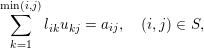 $$\begin{eqnarray}\mathop{\sum }_{k=1}^{\min (i,j)}l_{ik}u_{kj}=a_{ij},\quad (i,j)\in S,\end{eqnarray}$$
which corresponds to enforcing the property (11.1). A common convention for ILU factorizations is to fix the diagonal of the lower triangular  $L$ to one. For this convention, the generation of the incomplete factors is equivalent to solving a system of
 $|S|$ equations in
 $|S|$ unknowns.
The formulation (Chow and Patel Reference Chow and Patel2015)
 $$\begin{eqnarray}\displaystyle l_{ij} & = & \displaystyle \frac{1}{u_{jj}}\left(a_{ij}-\mathop{\sum }_{k=1}^{j-1}l_{ik}u_{kj}\right),\quad i>j,\end{eqnarray}$$
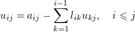 $$\begin{eqnarray}\displaystyle u_{ij} & = & \displaystyle a_{ij}-\mathop{\sum }_{k=1}^{i-1}l_{ik}u_{kj},\quad i\leq j\end{eqnarray}$$
allows us to derive a fixed-point iteration of the form  $x=G(x)$, where
 $x$ is a vector containing the unknowns
 $l_{ij}$ and
 $u_{ij}$ for
 $(i,j)\in S$. The equations are then solved by iterating the matrix entries in the form
 $$\begin{eqnarray}x^{(p+1)}=G(x^{(p)}),\quad p=0,1,\ldots ,\end{eqnarray}$$
starting with some initial  $x^{(0)}$ (Chow and Patel Reference Chow and Patel2015). As for traditional Gaussian elimination, it is also possible for the iterative algorithm generating the incomplete factors to exploit the symmetry of the system matrix. The iterative approach to a Cholesky factorization (IC) iterates the components according to
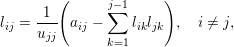 $$\begin{eqnarray}\displaystyle l_{ij} & = & \displaystyle \frac{1}{u_{jj}}\left(a_{ij}-\mathop{\sum }_{k=1}^{j-1}l_{ik}l_{jk}\right),\quad i\neq j,\end{eqnarray}$$
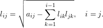 $$\begin{eqnarray}\displaystyle l_{ij} & = & \displaystyle \sqrt{a_{ij}-\mathop{\sum }_{k=1}^{i-1}l_{ik}l_{jk}},\quad i=j.\end{eqnarray}$$
For a suitable initial guess, it can be proved that the fixed-point iteration is locally convergent in the asymptotic sense (Chow and Patel Reference Chow and Patel2015). This in particular includes convergence for iteration schemes updating the distinct components in an asynchronous fashion (Frommer and Szyld Reference Frommer and Szyld2000), which is an essential aspect when parallelizing fixed-point iteration methods. In general, an iteration based on  $x^{(p+1)}=G(x^{(p)})$ can be parallelized by assigning each processor to compute a subset of the components of
 $x^{(p+1)}$ using values of
 $x^{(p)}$, such that each component is updated by exactly one processor. As all values of
 $x^{(p)}$ must generally be available before the computation of
 $x^{(p+1)}$ can start, this is called a synchronous iteration (Frommer and Szyld Reference Frommer and Szyld2000). In an asynchronous iteration, the computation of components of
 $x^{(p+1)}$ is started without ensuring that all values of
 $x^{(p)}$ are available, but the iteration uses, respectively, the latest value for the components of
 $x$ that are available. Convergence may be faster than the synchronous iteration because more updated values are used (e.g., Gauss–Seidel-type iteration compared to Jacobi-type) or may be slower than a synchronous iteration in the case when some components are rarely updated (Chow, Anzt and Dongarra Reference Chow, Anzt and Dongarra2015). In general, there may be a trade-off between parallelism and convergence: with fewer parallel resources, the asynchronous iterations tend to use ‘fresher’ data when computing updates; with more parallel resources, the iterations tend to use older data and thus converge more slowly. The advantage of iteration methods converging in the asynchronous sense is that it removes the need for performance-detrimental synchronizations in the implementations (Anzt, Tomov, Dongarra and Heuveline Reference Anzt, Tomov, Dongarra and Heuveline2013). It turns out that the iterative algorithm for computing incomplete LU factorizations carries a number of properties that make the algorithm attractive for high-performance computing (Chow et al. Reference Chow, Anzt and Dongarra2015).
∙ The algorithm is fine-grained, allowing for scaling to very large core counts, limited only by the number of non-zero elements in the factorization.
∙ The algorithm does not need to use reordering to enhance parallelism, and thus reorderings can be used that either enhance the accuracy of the incomplete factorization or the data locality in hardware.
∙ The bilinear equations do not need to be solved very accurately since the ILU factorization itself is only an approximation.
∙ The algorithm can use an initial guess for the ILU factorization, which cannot be exploited by conventional ILU factorization algorithms.
∙ The algorithm may be able to tolerate communication latencies and certain types of computation and communication errors due to its asynchronous nature.
Furthermore, the simplicity of the algorithm realizing the fixed-point iteration allows for efficient implementation on many-core accelerators: see Algorithm 21. In particular, it is possible to exploit the sparsity of the LU factors by storing the factors  $L$ and
 $U$ in CSR and CSC format, respectively, and the matrix
 $A$ in coordinate (COO) format (Chow et al. Reference Chow, Anzt and Dongarra2015). This matrix can also be regarded as a ‘task list’ as it determines in which order the components of
 $L$ and
 $U$ are updated. Changing the order of elements in this COO array controls the order of the updates, but the matrix ordering is preserved.
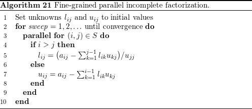
An implementation on Intel’s Xeon Phi architecture is evaluated in Chow and Patel (Reference Chow and Patel2015). In Chow et al. (Reference Chow, Anzt and Dongarra2015), an implementation, which is now part of the MAGMA-sparse open source software library,Footnote 16 is used to show how the algorithm succeeds in exploiting the computing power of a state-of-the-art NVIDIA GPU.
The parallelization concept used is based on assigning subsets of the components of  $x$ to GPU thread blocks. Each thread block updates the components of
 $x$ assigned to it (Chow et al. Reference Chow, Anzt and Dongarra2015). Within each thread block, the components of
 $x$ are updated simultaneously (in Jacobi-like fashion). As there are generally more thread blocks than the multiprocessors can execute in parallel, some thread blocks are processed before others, and thus update their components of
 $x$ before others. Thus some thread blocks within one fixed-point sweep may use newer data than others (in Gauss–Seidel-like fashion). Since there exists no fixed order in which the distinct blocks are updated, the iteration is considered to be ‘block-asynchronous’ (Anzt et al. Reference Anzt, Tomov, Dongarra and Heuveline2013). In traditional GPU computations, there is no defined ordering in which thread blocks are executed by the multiprocessors. However, on NVIDIA’s Kepler GPU generation the preferred scheduling order is consistent with the thread block numbering (Chow et al. Reference Chow, Anzt and Dongarra2015). Together with the fact that the matrix entries of
 $A$ are stored in COO format, this allows us assign how the elements are gathered into the thread blocks, and to control the order in which the elements are iterated. For fast convergence, the updates should be scheduled in dependency order. Different aspects play a role if optimizing for efficient hardware use. As the algorithm is memory-bound, one performance-critical goal is to maximize cache re-use. A first step to enhance cache re-use is to gather components that have similar dependencies in the same thread block. In the parallel GPU implementation, each thread updates one element
 $(i,j)\in S$. Each thread thus computes either
 $l_{ij}$ or
 $u_{ij}$ in equation (11.3) (Chow et al. Reference Chow, Anzt and Dongarra2015). For updating a component
 $l_{ij}$,
 $i>j$ (respectively
 $u_{ij}$,
 $i\leq j$), as well as the matrix element
 $a_{ij}$, all elements
 $l_{ik}$ of
 $L$ with
 $k<\min (i,j)$, and all elements
 $u_{kj}$ of
 $U$ with
 $k<\min (i,j)$ are required. Hence, this computation requires reading row
 $i$ of
 $L$ and column
 $j$ of
 $U$ (up to an upper limit) into local memory. This row and column may be re-used to compute other elements in
 $S$. Optimizing cache re-use is thus equivalent to partitioning the
 $(i,j)\in S$ among a given number of thread blocks such that threads in the thread block require, in aggregate, as few rows of
 $L$ or columns of
 $U$ as possible. Another way to view this problem is to maximize the number of times each row of
 $L$ and each column of
 $U$ is re-used by a thread block. In Chow et al. (Reference Chow, Anzt and Dongarra2015) this optimization problem is tackled by defining a ‘re-use factor’
 $f_{\text{re-use}}(l)$ for a thread block
 $l$ as
 $$\begin{eqnarray}f_{\text{re-use}}(l):=\frac{1}{2}\biggl(\frac{|S_{l}|}{m_{l}}+\frac{|S_{l}|}{n_{l}}\biggr),\end{eqnarray}$$
where  $|S_{l}|$ is the number of elements of
 $S$ assigned to thread block
 $l$, and where
 $m_{l}$ and
 $n_{l}$ are the number of rows of
 $L$ and columns of
 $U$, respectively, required by thread block
 $l$. The first term in the brackets is the average number of times that the rows are re-used, while the second is the average number of times that the columns are re-used (Chow et al. Reference Chow, Anzt and Dongarra2015). If the elements of
 $S$ are assigned arbitrarily to the thread blocks, then the re-use factor is 1 in the worst case (Chow et al. Reference Chow, Anzt and Dongarra2015). For problems arising from finite difference discretizations of partial differential equations, Chow et al. (Reference Chow, Anzt and Dongarra2015) derive the theoretical upper bound for the re-use factor
 $f_{\text{re-use}}(l)<s$ if an
 $s$-point stencil were used for discretizing a two- or three-dimensional problem. This indicates that larger re-use is possible for stencils of larger order (Chow et al. Reference Chow, Anzt and Dongarra2015).
(a) A  $6\times 6$ mesh using a five-point stencil partitioned into nine subdomains of size
 $2\times 2$. The corresponding matrix (b) orders rows and columns subdomain by subdomain. The bold edges in the mesh correspond to the non-zeros in the matrix marked with squares, and identify the elements assigned to one of the thread blocks. (c) The partitioning of the matrix after applying reverse Cuthill–McKee (RCM) and using 12 partitions.
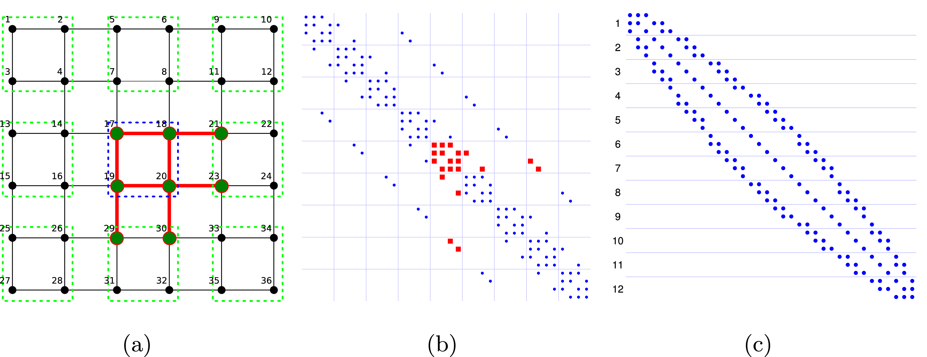
For those finite difference discretizations, re-use factors close to the upper bound can be achieved when using a domain decomposition into blocks with low anisotropy, and numbering the unknowns block by block. This results in a vector of unknowns where the adjacency of the components in the problem is preserved. Consequently, this blocking strategy helps in generating a task list order for updating the components in  $L$ and
 $U$ where components in the same thread block share dependencies (i.e., they are adjacent to the same vertices). Figure 11.1 visualizes this concept of blocking for the case of a five-point stencil discretization in two dimensions (Chow et al. Reference Chow, Anzt and Dongarra2015).
In practical GPU implementations, the cache re-use is larger than the theoretical bound. This is possible because cache can be shared between thread blocks (i.e., one thread block uses data brought into the L2 cache by another thread block: Chow et al. Reference Chow, Anzt and Dongarra2015), although this is not implied by the traditional GPU computing paradigms. Against this background it is beneficial to account for dependency similarities not only when assigning components to a thread block but also when ordering the thread blocks for the preferred execution order. When using a reverse Cuthill–McKee (RCM) ordering for the system matrix  $A$, which is usually beneficial to the approximation accuracy of incomplete factorizations (Duff and Meurant Reference Duff and Meurant1989), this can be achieved by forming blocks containing several rows and numbering the thread blocks from top to bottom: see Figure 11.1(c). From this figure it can be observed that each partition requires different rows of
 $L$ that are re-used within a thread block but not across thread blocks. Furthermore, partitions numbered nearby use a very similar set of columns of
 $U$, which may result in cache re-use of
 $U$ across thread blocks.
A different implementation aspect relevant for performance on streaming processors such as GPUs is the fact that significant thread divergence can occur if the partial sum (lines 5 and 7 of Algorithm 21) contains a different number of addends for components handled by the same warp. Minimizing warp divergence, however, conflicts with optimizing component assignment for cache re-use, and for a memory-bound algorithm data locality is more important (Chow et al. Reference Chow, Anzt and Dongarra2015).
A comprehensive analysis in Chow et al. (Reference Chow, Anzt and Dongarra2015) reveals that using RCM ordering of the matrix in combination with left–right and top-down ordering of the matrix entries in the task list and a top-down scheduling of the thread blocks is the preferred setup. In particular, it results in high intra- and inter-cache re-use, and succeeds in updating components in dependency order, which is key to good performance and fast convergence, respectively.
For the convergence analysis, the fixed-point iterations were started taking the upper and lower triangular factors of the matrix  $\tilde{A}$ as an initial guess, where
 $\tilde{A}$ is the system matrix
 $A$ symmetrically scaled to a unit diagonal. This initial guess has been shown to allow for good convergence if no natural initial guess, such as a previous factorization to a similar system, is available (Chow and Patel Reference Chow and Patel2015).
For a set of test matrices taken from the University of Florida Matrix Collection (UFMC: Davis and Hu Reference Davis and Hu1994), Chow et al. (Reference Chow, Anzt and Dongarra2015) compare the fixed-point based ILU generation to NVIDIA’s cuPARSE libraryFootnote 17 in version 6.0, which uses level scheduling to exploit the hardware parallelism. A good metric for evaluating the approximation accuracy of a preconditioner is the convergence of a top-level iterative solver using the generated preconditioner (Chow and Patel Reference Chow and Patel2015). The left side of Table 11.1 (taken from Chow et al. Reference Chow, Anzt and Dongarra2015) reveals that for a few sweeps of the fixed-point iteration, the PCG solver iteration count is reduced to values similar to using conventionally generated ILU. For details of the test matrices see Chow et al. (Reference Chow, Anzt and Dongarra2015). The right side of Table 11.1 shows the timings for IC computed using NVIDIA’s cuSPARSE library, and for five fixed-point iteration sweeps using an NVIDIA Kepler K40 GPU. Five sweeps have proved to be sufficient for accurate preconditioner generation, and their execution time is typically only a fraction of the runtime needed by the traditional approach.
PCG solver iteration counts using preconditioners constructed with up to five sweeps, and timings for five sweeps. IC denotes the exact factorization computed using NVIDIA’s cuSPARSE library. The speedup shown is that of five sweeps relative to IC.
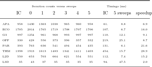
11.2 Approximate triangular solves
Besides the derivation of the incomplete factors, the application of an incomplete factorization preconditioner via forward and backward triangular solves also poses a computational challenge (Park, Smelyanskiy, Sundaram and Dubey Reference Park, Smelyanskiy, Sundaram and Dubey2014). As in the factorization case, the dependencies result in an inherently sequential algorithm that makes it difficult to exploit the parallel computing power available in today’s architectures. As the preconditioner applications impact the performance of every iteration of a top-level iterative solver, the acceleration of sparse triangular solves may be considered even more important, and is the subject of significant research efforts. Similarly to the factorization problem, it is possible to get some parallelism from level scheduling components that are independent (Saad Reference Saad2003). However, depending on the sparse matrix, there may be a very large number of levels or not enough work within a level to efficiently use highly parallel architectures such as GPUs. Different groups have tried to increase the parallelism obtained from level scheduling at the cost of a less accurate preconditioner (Anderson and Saad Reference Anderson and Saad1989, Saltz Reference Saltz1990, Hammond and Schreiber Reference Hammond and Schreiber1992). Nevertheless, efficient implementations on state-of-the-art hardware still pose a challenge (Mayer Reference Mayer2009, Wolf, Heroux and Boman Reference Wolf, Heroux and Boman2011, Naumov Reference Naumov2011). A different approach to parallelizing sparse triangular solves is to use partitioned inverses (Alvarado and Schreiber Reference Alvarado and Schreiber1993, Pothen and Alvarado Reference Pothen and Alvarado1992). The idea is to write the matrix as the product of sparse triangular factors; each triangular solve is then a sequence of sparse matrix vector multiplications. Similar to this, the use of a sparse approximate inverse for a triangular matrix has also been considered (van Duin Reference van Duin1996, Tuma and Benzi Reference Tuma and Benzi1998), as well as the idea of approximating the inverse ILU factors via a truncated Neumann series (Tuma and Benzi Reference Tuma and Benzi1998, van der Vorst Reference van der Vorst1982). Finally, there exists the idea of using relaxation methods for approximate triangular solves. Chow and Patel (Reference Chow and Patel2015) investigated the use of Jacobi sweeps for approximate sparse triangular solves on the Intel MIC architecture. The Jacobi iteration for solving  $Ax=b$ can be written as
 $$\begin{eqnarray}\begin{array}{@{}l@{}}x^{k+1}=D^{-1}(b-(A-D)x^{k}),\\ x^{k+1}=D^{-1}b+Mx^{k},\end{array}\end{eqnarray}$$
where  $D$ is the diagonal part of
 $A$ (Anzt Reference Anzt2012). For the triangular systems that arise in the context of incomplete factorization preconditioning, the iteration matrices
 $M_{L}$ and
 $M_{U}$ for the lower and upper triangular, respectively, can be derived as (Anzt, Chow and Dongarra Reference Anzt, Chow, Dongarra, Träff, Hunold and Versaci2015)
 $$\begin{eqnarray}\begin{array}{@{}l@{}}M_{L}=D_{L}^{-1}(D_{L}-L)=I-L,\\ M_{U}=D_{U}^{-1}(D_{U}-U)=I-D_{U}^{-1}U,\end{array}\end{eqnarray}$$
where  $D_{L}$ and
 $D_{U}$ denote the diagonal parts of the triangular factors
 $L$ and
 $U$, and
 $I$ is the identity matrix. Obviously,
 $M_{L}$ is strictly lower triangular and
 $M_{U}$ is strictly upper triangular, which implies that the spectral radius of both iteration matrices is zero (Golub and Van Loan Reference Golub and Van Loan1996). This is a sufficient condition for an asynchronous iteration method to converge in the asymptotic sense (Frommer and Szyld Reference Frommer and Szyld2000). Anzt et al. (Reference Anzt, Chow, Dongarra, Träff, Hunold and Versaci2015) compared approximate triangular solves based on Jacobi with triangular solves based on block-asynchronous Jacobi. As previously mentioned, block-asynchronous fixed-point iterations can provide faster convergence if the dependency order is reflected in Gauss–Seidel-type updates (Anzt et al. Reference Anzt, Tomov, Dongarra and Heuveline2013). In the GPU implementation considered, the set of unknowns is partitioned into blocks, components in a block are updated in synchronous Jacobi-like fashion, and the distinct blocks are scheduled onto the multiprocessors. The idea is to adapt the preferred scheduling order to the system characteristics. That is, schedule the blocks top-down for the lower triangular system
 $Ly=b$ and bottom-up for the upper triangular system
 $Ux=y$. For the incomplete triangular factors (ILU(0)) of a finite difference discretization of the Laplace problem in three dimensions discretized using a 27-point stencil on a
 $64\times 64\times 64$ grid, Figure 11.2(b, d) visualizes the effect of dependency-aware thread block scheduling (Anzt et al. Reference Anzt, Chow, Dongarra, Träff, Hunold and Versaci2015). As expected, scheduling the thread blocks top-down for the lower triangular system and bottom-up for the upper triangular system results in faster convergence. Scheduling against the dependency order, no convergence-relevant Gauss–Seidel updates are scheduled, and the convergence rate is comparable to the Jacobi method (Anzt et al. Reference Anzt, Chow, Dongarra, Träff, Hunold and Versaci2015). Figure 11.2(b, d) relates the relative residual norm to the runtime when executing the different approximate triangular solvers, all part of the MAGMA-sparse library, on an NVIDIA Kepler K40 GPU. Although dependency-aware block-asynchronous Jacobi achieves a higher convergence rate, the time-to-solution winner is cuSPARSE-based Jacobi. The reason stems from the high optimization level of the sparse matrix vector product that this implementation is based on. However, from comparing the convergence rates for synchronous and block-asynchronous Jacobi, it can be deduced that applying the same level of optimization to the kernel for block-asynchronous Jacobi would also make it superior with respect to the performance metric (Anzt et al. Reference Anzt, Chow, Dongarra, Träff, Hunold and Versaci2015).
Solving the sparse triangular systems for the lower and upper triangular ILU(0) factors of the Laplace problem in three dimensions using a 27-point stencil discretization on a  $64\times 64\times 64$ grid. Convergence (a, c) and runtime (b, d) of synchronous Jacobi and block-asynchronous Jacobi (averaged results).
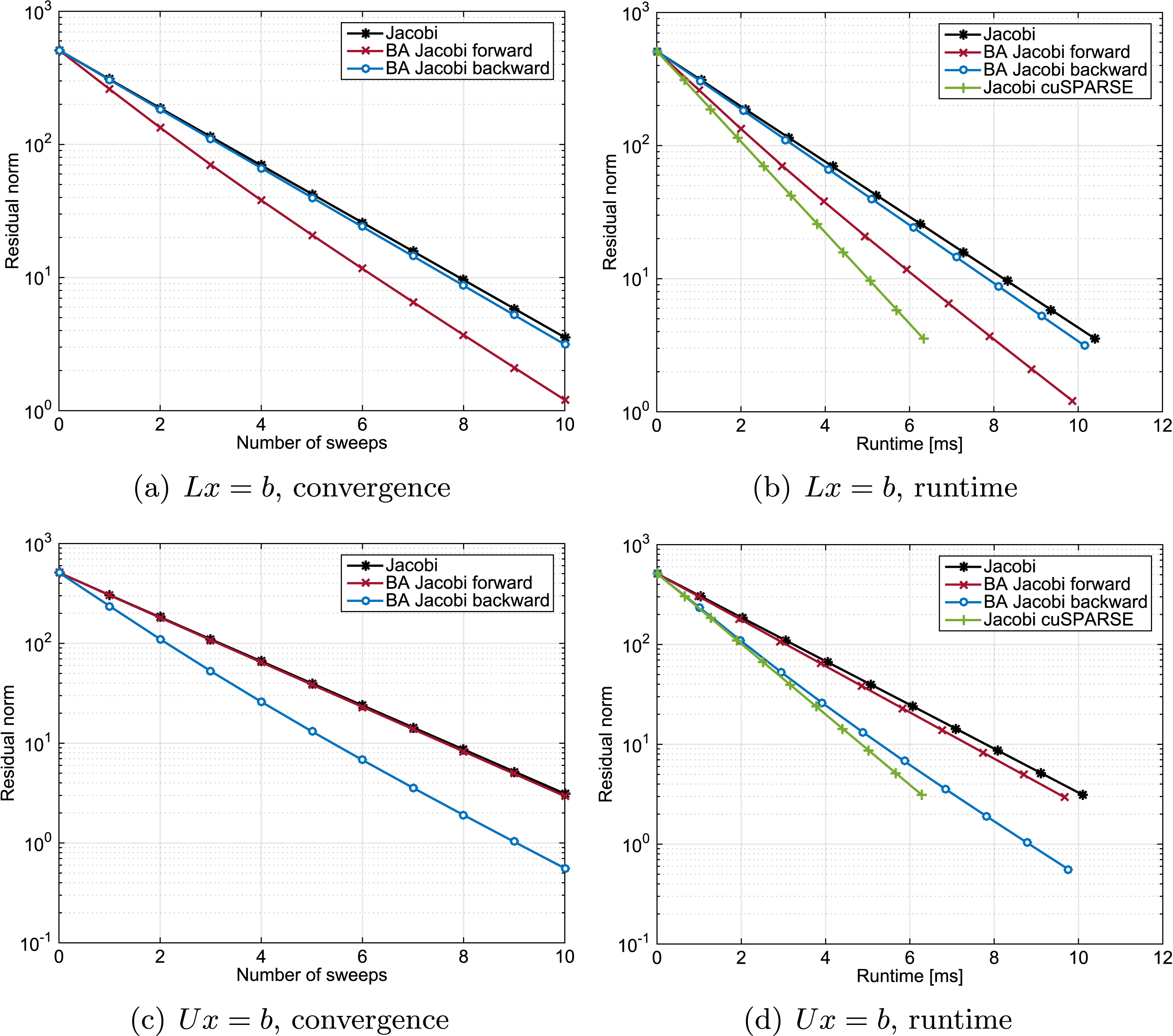
Compared to the level scheduling sparse triangular solves of NVIDIA’s cuSPARSE library, one sweep of the approximate triangular solves based on Jacobi or block-asynchronous Jacobi is typically between one and two orders of magnitude faster (Anzt et al. Reference Anzt, Chow, Dongarra, Träff, Hunold and Versaci2015). In contrast to a deterministic Jacobi method, using block-asynchronous Jacobi for the approximate triangular solves requires the top-level iterative method to be tolerant to a changing preconditioner. The reason is that, despite the preferred scheduling order, a fixed execution order of the thread blocks cannot be guaranteed. An example for a Krylov iterative method capable of handling a changing preconditioner is the flexible GMRES (FGMRES: Saad Reference Saad1993). Chow and Patel (Reference Chow and Patel2015) show that a few sweeps are sufficient to provide preconditioner accuracy comparable to exact triangular solves based on level scheduling. As expected from the convergence analysis in Figure 11.2, this is no different for the block-asynchronous Jacobi: see Anzt et al. (Reference Anzt, Chow, Dongarra, Träff, Hunold and Versaci2015). Finally, replacing the exact triangular solves with approximate triangular solves succeeds in accelerating the complete solution process of the top-level iterative solver (Anzt et al. Reference Anzt, Chow, Dongarra, Träff, Hunold and Versaci2015).
12 Conclusion
The past decade has been marked by significant innovation in linear algebra algorithms and software, stimulated by the proliferation of multicore processors and hardware accelerators, and the overall increase in the level of parallelism required to achieve high performance. New or improved algorithms have been developed for the solution of basic problems in linear algebra, including linear systems of equations, least-squares problems, singular value problems and eigenvalue problems. These algorithms utilize memory hierarchies better than their predecessors, expose higher levels of parallelism, are more suitable for dataflow scheduling, consume less network bandwidth, and tolerate larger network latencies. Most importantly, these innovations have resulted in high-quality implementations provided in the form of robust software packages for multicore systems, hybrid (multicore + accelerator) systems, and distributed memory systems (with multicore processors and accelerators). As the numerical computing community continues to ramp up for exascale computing, there is no reason to believe this pace will slow – even in the face of the great challenges that lie ahead.