











No CrossRef data available.
Simplified time series representations for efficient analysis of industrial process data
Published online by Cambridge University Press: 07 November 2003
Abstract
The data storage capacities of modern process automation systems have grown rapidly. Nowadays, the systems are able to frequently carry out even hundreds of measurements in parallel and store them in databases. However, these data are still rarely used in the analysis of processes. In this article, preparation of the raw data for further analysis is considered using feature extraction from signals by piecewise linear modeling. Prior to modeling, a preprocessing phase that removes some artifacts from the data is suggested. Because optimal models are computationally infeasible, fast heuristic algorithms must be utilized. Outlines for the optimal and some fast heuristic algorithms with modifications required by the preprocessing are given. In order to illustrate utilization of the features, a process diagnostics framework is presented. Among a large number of signals, the procedure finds the ones that best explain the observed short-term fluctuations in one signal. In the experiments, the piecewise linear modeling algorithms are compared using a massive data set from an operational paper machine. The use of piecewise linear representations in the analysis of changes in one real process measurement signal is demonstrated.
Information
- Type
- Research Article
- Information
- Copyright
- 2003 Cambridge University Press
1. INTRODUCTION
Analysis, supervision, and control of the tasks of a large-scale industrial process are often complicated either by partially unknown dependencies within the process or by incomplete understanding of the process behavior due to many factors that affect it. On the other hand, the processes of today are equipped with many sensors that frequently carry out measurements from the process with high sample rates and store them in databases of the automation systems. The data histories may even be years long, and they are typically rarely utilized (Wang, 1999).1
However, one has to be careful in the analysis of process data: if the process has been modified, the dependencies may also have changed and data recorded before the changes have became useless.
As many process signals contain little essential information, they can be analyzed more efficiently by describing them in a more compact form. Several possible ways to obtain simplified representations for process data have been reported in the literature. Filtering methods (Love & Simaan, 1988) and multilayer perceptron networks (Rengaswamy & Venkatasubramanian, 1995) have been used to decompose process signals into primitives for syntactic pattern recognition. Other alternatives include triangular episodes (Cheung & Stephanopoulos, 1990) and multiscale representation using wavelet transform (Bakshi & Stephanopoulos, 1994). Wavelets have been found to be especially useful in many tasks such as process diagnosis (Vedam & Venkatasubramanian, 1997; Chen et al., 1999), analysis and display of data (McLeod et al., 1998), and data compression (Nesic et al., 1996). The wavelet transform produces a multiscale representation of data that has good localization in both time and frequency. Thus, it is well suited for modeling process data that typically contain events on multiple scales.
Another characteristic feature of process data is that they usually contain many measured variables, that is, the dimensionality of the data is high. On the other hand, the variables are usually highly dependent and dimension reduction without significant loss of information can be carried out. The variables resulting from dimension reduction, so-called latent variables, are traditionally obtained using principal component analysis (PCA) or partial least squares (PLS). Both methods use second-order statistics of the data in the dimension reduction and produce orthogonal latent variables that are linear combinations of the original ones. PCA treats all the variables equally and performs dimension reduction that minimizes loss of total data variance. PLS is closely related to PCA, but it seeks to maximize covariance between input and output variables instead. For a survey of PCA and PLS techniques for process data, see, for example, Kourti and MacGregor (1995). PCA can also be used to monitor a single measurement signal in multiple scales using the wavelet transform (Bakshi, 1999; Zhang et al., 1999). A new and emerging technique for computation of latent variables is independent component analysis (ICA), which finds latent variables that are, according to the name of the method, independent of each other. For a survey on ICA, see Hyvärinen (1999) and for an illustration of using ICA for process data, see Li and Wang (2002). After dimension reduction of data using PCA, PLS, or ICA, any available method can be used to compute a simplified representation of the latent variables. In that case, the amount of data is reduced in two different ways: first the dimension is reduced, and then simplified representations are computed for the latent variables.
The simplification method considered in this paper is piecewise linear modeling of signals. In the modeling, the time axis is divided into segments of varying size and each signal segment is modeled using a linear model of its own. Polynomials of any degree can naturally be used, but the first-order polynomial is sufficient to depict the phenomena of process data that are typically of interest: impulses, ramps, and steps. The piecewise linear modeling approach is simple and computationally efficient, and it also makes it possible to easily ignore periods that contain faulty data. The last property is a necessity in real-world applications; for many other methods mentioned above, dealing with such data is not straightforward. Further, piecewise linear modeling can also be used to obtain signal representation in many resolutions by using different numbers of linear models (segments) in the signal representation. However, in this case the concept of resolution is different from scale in the wavelet transform. The piecewise linear modeling finds the underlying trend in data by optimizing a global error function in the time domain whereas in the wavelet transform time and frequency axes are both divided in multiple levels to obtain the simplified representation.
The two most commonly used error norms in piecewise linear modeling are L2 and L∞. In the former case, the optimal algorithm is given in Bellman (1961) and in the latter case in Imai and Iri (1986). Due to the fact that in our application we are mainly dealing with noisy signals, the L2 norm is used. Because the computation time of the optimal solution in the L2 norm case is quadratic with respect to the number of samples in the time series, the algorithm is computationally too heavy for a very long series. During the past decades, several fast heuristic methods have been proposed to overcome the problem (Cantoni, 1971; Pavlidis, 1973, 1974; Wu, 1984; Keogh & Smyth, 1997; Guralnik & Srivastava, 1999; Himberg et al., 2001).
Piecewise linear modeling is closely related to the change detection problem (Basseville & Nikiforov, 1993) that is typically encountered in on-line applications. A change in a signal is, for example, a symptom of a fault in a machine. Another related application is signal compression, which is widely used, for instance, in medical applications (Konstantinides & Natarajan, 1994; Nygaard et al., 2001). Feature extraction by piecewise linear modeling can be seen as signal compression in which noise and irrelevant minor variations are discarded but all the essential signal change points are retained as faithfully as possible. To assure this, the signals are “oversegmented” by using more segments than necessary to depict the main characteristics of the signal. Selection of the number of segments is usually based on a priori information on the nature of the signal.
In this article, fast heuristic methods for piecewise linear modeling of signals are considered. Typically, process measurement signals contain values that are either not available or known to be invalid based on some external information. Still, little attention has been paid to modeling such data. For instance, this aspect has not been extensively considered in any of the works mentioned above.
An important contribution of this paper is a detailed description of all the operations that are required to build a piecewise linear model for a signal, which may contain missing and erroneous measurements. The paper starts with a novel preprocessing scheme in which the artifacts mentioned above can be dealt with in an effective manner. Then, a number of existing segmentation algorithms are reviewed and outlined. For each of these, modifications due to dealing with imperfect data are pointed out. Also, fast computation of the line fit and error for an arbitrary segment in constant time is described in detail. In order to shed some light on the analysis methods, use of the piecewise linear models in process diagnostics using subsequence matching is considered. A novel framework for the discovery of dependencies in process data is presented.
In the experiments, a large data set from an operational paper machine with about 600 time series (100,000 points each) is used. The objective is to find out which piecewise linear modeling algorithm is best suited for the data and how close in accuracy to the optimal solution the heuristic algorithms can get. An example of process diagnostics using piecewise linear models is also presented.
The rest of the paper is organized as follows. Section 2 includes a detailed description of the preprocessing scheme. Piecewise linear modeling of preprocessed data is considered in Section 3. Section 4 presents the proposed process diagnostics procedure. In Section 5, experiments using the real-world data set are reported. Section 6 summarizes the paper and contains conclusions based on the results.
2. PREPROCESSING OF MEASUREMENT SIGNALS
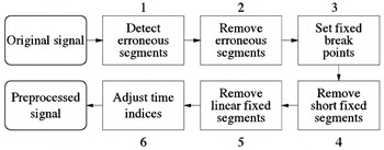
A time series (signal) is denoted here by x(1), x(2),…, x(N). Typically, a measurement signal obtained from a real industrial process contains two kinds of defects: erroneous and missing values. In order to find a proper piecewise linear model for the signal, it is sensible to ignore these anomalies by removing them from the signal before modeling. However, the time indices of the removed regions need to be stored, because they are needed when the model is used later. The phases of preprocessing that carry out data cleansing are presented in Figure 1.

Phases 1–6 of the preprocessing from original (raw) data to preprocessed data.
In phases 1 and 2, erroneous segments are determined and removed from the data. In practice, it is usual that part of the values are missing or some existing values are known to be invalid based on available external information. In process data, the former may be due to a fault in the database system that stores the data. A simple example on the latter is “jamming” of a sensor reading to a constant value, which may be a consequence of breakdown of a measurement sensor.
In phase 3, the regions removed in phase 2 are reconsidered. If there is a reason to believe that the signal properties have changed during a removed region, a discontinuity point, or fixed break point (Tfix), is set in the time series at the last valid point before the removed region. A fixed break point, which may not be moved later in the piecewise modeling phase, permanently divides the time series into fixed segments. For example, during shutdown of a process, measurement sensors are often cleaned, repaired, or calibrated, which changes the characteristics of the device. Therefore, it may be justified to start a new segment after the shutdown. Another possible criterion for setting a fixed break point is a simple heuristic: if the length of the removed segment exceeds some predefined threshold, a break point is set.
In phase 4, fixed segments that consist of less than 4 points are removed, because they cannot be further divided into two linear segments. Also, the fixed segments that can be perfectly modeled using a single line are removed in phase 5.
Finally, in phase 6, the time indices are adjusted. At this point we change the notation so that the number of remaining samples in the time series is from now on denoted by N. Also, the time indices of the new, preprocessed time series are denoted by t, t = 1,…, N and the old, original values by t′(1),…, t′(N). The number of fixed break points (which is equal to the number of fixed segments) is denoted by k′ and the fixed break points by T1fix,…, Tk′fix.
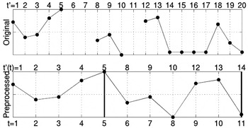
Figure 2 shows a toy example of the preprocessing procedure. In phases 1 and 2, the missing values at time instances 6–7 and 11 and “jammed” values at time instances 15–17 are detected and deleted. In phase 3, removal of two successive points is considered to produce a fixed break point; two break points are set at time instances 5 and 14. In phase 4, the short segment at the time instances 18–20 is removed. In phase 5, nothing is done, because no linear segments exist. In phase 6, the time indices are adjusted: the original time labels t′(t) of the remaining samples are shown above the preprocessed signal in Figure 2. Below the figure, the new time labels t are shown. The remaining signal consists of two fixed segments, intervals 1–5 and 8–14 of the original signal.

The original signal (top) and the preprocessed signal (bottom) with corresponding old time labels on top and new time labels at the bottom. The two thick lines denote the fixed break points.
3. PIECEWISE LINEAR MODELING OF PREPROCESSED SIGNALS
In piecewise linear modeling, the objective is to divide the time series into k separate segments n = 1,…, k, and approximate each of these by a linear model

Thus, the model consists of time indices of the last samples of the segments Tn (i.e., break points) and slope (an) and constant terms (bn) for each segment. It is assumed that the time series is corrupted by i.i.d. additive Gaussian noise with zero mean. Thus, given the break points, minimization of the total error (in this notation T0 = 0),

gives the maximum likelihood estimates for the line parameters (Bishop, 1995). Fast computation of the error and line parameters for an arbitrary segment in constant time after one pass through the time series is described in Appendix A. However, now we concentrate on the segmentation algorithms, which determine the positions of the break points.
3.1. Segmentation algorithms
Below, the time series segmentation algorithms are presented and outlined. In each case, first the baseline algorithm is introduced and then the required modifications due to fixed segments produced by the preprocessing phase are described.
3.1.1. Optimal algorithm
The optimal piecewise linear model can be computed using the well-known dynamic programming principle (Bellman, 1961). Later, the same approach was used in, for example, segmentation of speech (Xiong et al., 1994; Prandoni et al., 1997) and mobile phone data (Himberg et al., 2001). The computational complexity of the algorithm is of order O(kN2), where k is the number of segments and N is the number of samples in the time series. The algorithm is incremental: before a time series is divided into k segments, all divisions to 1,…, k − 1 segments have to be computed.
Baseline algorithm
- Set l = 1.
- Compute optimal l + 1 segmentations for all segments 4
≤ t < N:
For each t, store the break point T, error Eoptl+1(1, t) and line fit parameters.

- Set l = l + 1. If l > k, quit; otherwise, go to 2.
Modifications due to fixed segments. The dynamic programming principle needs to be applied twice. On one hand, it is used to optimally divide each fixed segment into subsegments; on the other hand, it is used to find optimal segmentation for a group of adjacent fixed segments.
Let us assume that a time series has been divided into k′ fixed segments in the preprocessing and the time series is to be divided optimally into k > k′ segments.
- Divide the first fixed segment optimally into i = 1,…, k − k′ + 1 segments using the dynamic programming algorithm. Store the corresponding costs Eopti(1, T1fix), line fit parameters, and break points.
- Set l = 2.
- Divide the lth fixed segment optimally into i = 1,…, k − k′ + 1 segments using the dynamic programming algorithm. Store the corresponding costs Eopti(1, T1fix), line fit parameters, and break points.
- Compute the optimal segmentations for the l first fixed
segments s(1, Tlfix)
into j = l,…, k −
k′ + l segments:
Store the corresponding costs Eoptj(1, Tlfix), line fit parameters, and break points.
- Set l = l + 1. If l > k − k′, quit; otherwise go to 3.
When there are fixed break points, finding the optimal solution is actually speeded up, because the search space is smaller. It is not difficult to conclude that the speed-up is proportional to the number and length of the fixed segments and it is at most the number of fixed segments. As far as we know, the algorithm above has not been suggested elsewhere.
3.1.2. Fast heuristic algorithms
The computation time of the optimal solution is intolerable when the number of points in the time series is large. In the following, four fast heuristic algorithms that typically end up in a local minimum of the error function [Eq. (2)] are outlined. All the algorithms are deterministic and have computational costs that are linear with respect to the length of the time series.
Uniformly spaced break points. The simplest way is to select the break points uniformly in time. This choice is naturally very fast but typically produces poor results, because it completely ignores the structure of the time series.
Baseline algorithm. Formally, computation of break points can be written2
Here

; denotes the greatest integer that is ≤x.

The model is complete after each segment is computed from a linear model.
Modifications due to fixed segments. In the presence of fixed segments, one can think of several strategies to set the break points. We suggest that the break points should be uniformly set in the sequence 2,…, T1fix − 2, T1fix + 2,…, T2fix − 2,…, Tk′−1fix + 2,…, N − 2, which guarantees that no segment with less than two points can result and no break point can overlap with a fixed break point.
Top-down. The top-down approach used in this article was suggested in Guralnik and Srivastava (1999). The algorithm starts by splitting the whole time series optimally in two segments. Then, the segment optimal split of which most reduces the total error is split until k, the desired number of segments, are obtained.
Baseline algorithm
- Set l = 1.
- Split the segment i optimal split of which (at point
T) most decreases the error:
Discard the old error Ei and line fit parameters. Store the new ones with the new break point T.
- Set l = l + 1. If l < k, go to 2; otherwise, quit.
Modifications due to fixed segments. At the first step of the algorithm, l is set to k′; the segmentation begins with fixed segments as initial segments.
Bottom-up. In the bottom-up approach, the time series is first divided into segments of length 2. (If the number of points in the time series is odd, the length of the last segment is 3.) At each step of the algorithm, two of the existing segments are merged until k, the desired number of segments, has been reached. A model similar to the one described here was used in Keogh and Smyth (1997).
Baseline algorithm
- Set number of segments l =
.
- Initialize the break points in such a way that each segment contains two samples: Tn = 2 · n, n = 1,…, l − 1; Tl = N. Set En = 0, n = 1,…, l.
- Merge the two segments i and i + 1 that least
increase the total error:
Discard the ith break point Ti, old errors (Ei and Ei+1), and line fit parameters of ith and (i + 1)th segments and store the new ones.
- Set l = l − 1. If l > k, go to 3; otherwise, quit.
Modifications due to fixed segments. Initially, each fixed segment is divided into segments of length two. Thus, all the segments that have an odd number of samples will thus have three points in the last initial segment. Also, it has to be checked that two segments on both sides of a fixed break point are never merged.
Iterative/Split-and-Merge Approach. Some quite similar iterative and split-and-merge approaches have been suggested in the literature (Pavlidis, 1974; Hawkins, 1976; Himberg, 2001). We adopted the basic idea of the global iterative replacement (GIR) algorithm proposed in (Himberg, 2001). The main difference is that, in the original GIR, the break points to be removed were selected in random or sequential order. We always remove the one that gives the best reduction in model error. At each iteration of the algorithm, the break point that is least necessary in the sense of modeling error is moved to a place where the benefit is greatest.
Baseline algorithm
- Initialize the k break points.
- Select the break point Ti, the removal
of which produces the least increase in the total error:
- Select the segment j, the optimal split of which most
decreases the total error:
- If ΔEremove + ΔEsplit ≤ 0, quit. Otherwise, remove the break point Ti selected at step 2 and split the segment j that was selected at step 3. Update the errors and line fit parameters and go back to 2.
Modifications due to fixed segments. It is necessary to check that the GIR does not remove a fixed break point.
4. UTILIZATION OF THE MODEL
The piecewise linear models have three advantages in analysis of process data.
- Data compression. Each segment n requires three parameters: break (or end) point (Tn), slope term (an), and constant term (bn). Thus, memory requirement of a model for one signal is 3k, where k is the number of segments. For example, in our application this aspect is remarkable, because after piecewise linear modeling it is possible to keep all the models in the main memory of a standard PC at the same time.
- Removal of noise and irrelevant minor variations in the signals.
- Faster computation. If the number of segments is small with respect to the number of data points, many simple operations like computation of the average of a segment can be speeded up.
In the following section, a procedure for process diagnostics is roughly described. It can be used either to find signals that best explain variations in one signal of interest or to indicate which signals react to a change in the signal of interest. Even though in all formulas and notations the values of original time series are used, it is a very straightforward process to use the approximations given by the piecewise linear models instead.
The whole procedure is based on matching of subsequences and is aimed at the discovery of novel linear relationships in the data. Thus, in the matching, there is a transformation where shifting and linear scaling of signals is allowed (Chu & Wong, 1999). However, the concept can easily be used as well with other kinds of transforms that are suggested in the literature, for example, the discrete Fourier transform (Faloutsos et al., 1994).
4.1. Process diagnostics procedure
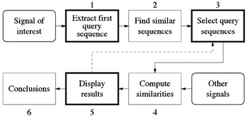
The starting point of the analysis is a short-term fluctuation, for example, a change of level, in a process signal of interest, which is denoted here by x0(t), t = 1,…, N. The six phases of the diagnostics procedure are shown in Figure 3. Three of them require interaction with the user. More detailed descriptions of the steps of the analysis are given below.

The six phases of the process diagnostics procedure. Phases 1, 3, and 5 require user interaction and are emphasized using a thick line.
The query sequenceq0 = [x0(t0),…, x0(t0 + L − 1)]T that contains the interesting pattern is extracted manually from the whole signal in phase 1.
3In order to keep the notation simple, vector notation is used in this section for sequences.

.
In phase 2, sequences of length L that are similar to q0 in the sense of Euclidean distance are looked for in x0(t). The search strategy is such that first the best matching sequence in the whole signal is located and labeled as used. After this, no other query sequence may overlap with this sequence. Then, the best matching sequence in the remaining signal is located and so on, until a continuous sequence of length L that consists of unoccupied points can no longer be extracted. Formally, the starting point of the mth query sequence is computed by

where

is the vector [x0(t),…, x0(t + L − 1)]T with offset shifted to zero and ∥·∥2 denotes the Euclidean norm. The vector

that gives the minimum of Eq. (3) is denoted by

. If one is interested in changes with the same scale as

, the scaling factor w0, m is set to 1. Setting w0, m to

finds similar changes on different scales and inverse sequences, because w0, m may be negative. After all possible M query sequences have been found, they are all concatenated into a query vector

.
In phase 3, the Q is pruned. In practice all the M query sequences of Q are not appropriate matches. Often, only the best ones are worth considering. Also, a small distance between two sequences does not necessarily agree with the human intuition of similar sequences. Therefore, feedback from the user is used to select only some of the query sequences for further inspection. The indices of the selected sequences are denoted by c(1),…, c(M′). The new, pruned query vector is thus

In phase 4, similarities between the query vector and the corresponding parts of all the other signals are computed. The phase starts with selection of minimum (dmin) and maximum delay/advance (dmax) values. If the goal is to find a reason for a change in a signal, one should look back in time and set dmax to 0 and dmin to some suitable negative value that is the longest possible delay from occurrence of any event to the detected change. Correspondingly, if one is interested in finding signals where changes in x0(t) are reflected, dmin should be set to 0 and dmax to some suitable positive value. Naturally, selection of dmin and dmax depends on the application.
Next, all the other signals xi(t) (where i = 1,…, P denotes the number of the signal) are considered one at a time. The match vectors of the ith signal are defined by

The match vector consists of concatenated match sequences

the notation

denotes the sequence sn, di with offset moved to zero.
Now the similarity, that is, the distance between the query vector and the match vector can be computed. It is given by

where
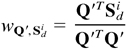
is a scaling factor that minimizes the distance between Q′ and Sdi. The value of d that minimizes the distance is an estimate of the delay or advance between events in Q′ and Si.
In phase 5, the results are shown to the analyst. The matches with the smallest distance between the match and query are shown first. At this stage it may become apparent that, for instance, based on some external information, some query sequences should be deleted and/or added. This is illustrated in Figure 3 by an arrow that returns to the selection of query sequences; the diagnostics procedure is thus iterative. Finally, in phase 6, conclusions are made. It is possible that the obtained results give rise to consideration of some other signal and a return to the beginning of the whole diagnosis procedure.
5. EXPERIMENTS
The experimental part is organized in the following way. The data set used in the experiments is described in Section 5.1. The evaluation of the performance of the piecewise linear modeling algorithms is reported in Section 5.2. The section is further divided into two parts: comparison of the heuristic algorithms with each other and comparison of the heuristic algorithms with the optimal solution by dynamic programming. The objective of the former test was to find out which method or methods are best suited for the data set used. The latter test was carried out to find out how close to the optimal solution the heuristic algorithms could get; unfortunately, for computational reasons only a fraction of the whole data set could be used in that test. In the end of the experimental part, in Section 5.3, an example of process diagnostics procedure (described in Section 4.1) in which the piecewise linear approximations were utilized is presented.
5.1. Data set
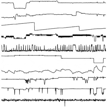
In the experiments, a massive real-world data set that consisted of 629 signals with 107,029 points each was used. Each signal was acquired from a database of a paper machine using 10-min resolution. Hence, the data described the behavior of the machine during about 743 days, which is >2 years. In order to get an impression of the signals, parts of 10 different signals that are typical of the process are shown in Figure 4.

Ten examples of the signals used in the experiments. Each plot contains 1000 points from one signal.
Before the experiments could be carried out, the data had to be preprocessed. Initially, empty signals and signal duplicates were removed. Then, the signals were preprocessed as presented in Section 3: all segments that had six or more successive constant values or three or more successive missing values were removed from the signals. Also, signals with less than 10,000 valid points were left out of the experiments. Finally, there were 489 signals left.
5.2. Evaluation of the piecewise linear modeling algorithms
Two things that were of interest for each algorithm were accuracy and computation time, which are both important when implementation of the algorithms is considered. The accuracy was measured by means of modeling error, that is, the sum of squared errors [Eq. (2)] and the computation time as CPU seconds. All the tests were carried out in Matlab 5.3 (The MathWorks, Inc., 1999) using a Compaq AlphaServer GS160. Because the implementations were not aggressively optimized, all the CPU times presented below should be considered merely indicative rather than as absolute truth.
In all experiments, the average number of segments per 100 signal points (which is referred to below as resolution of a model) was varied from 1 to 10. Even though algorithms whose error functions also contain a penalty term for model complexity (Djurić, 1994; Oliver et al., 1998) exist, we did not try to determine the “correct” number of segments. Our goal was only to reduce the number of data points from N to k to make it possible to use computationally demanding analysis methods after feature extraction.
5.2.1. Comparison of the heuristic algorithms
The heuristic algorithms were compared with each other using the whole data set. First, the resolution was set to 1. Then, the signals were modeled using uniform, bottom-up, and top-down algorithms. The obtained models were also fine-tuned using the GIR algorithm. Thus, six models for all signals were computed. For each signal, the minimum error (Emin) was determined among the six errors obtained by different algorithms. Then, the six errors were scaled in the following way (in order to make all the errors between different signals comparable):
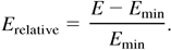
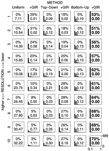
The same procedure was repeated using the next resolution until all resolutions were used. Histograms of the relative errors of all signals for all methods and resolutions are shown in Figure 5.

A comparison of the fast heuristic algorithms. Each plot is a histogram of relative errors that fall within the range [0, 1] for all signals using a fixed method at a fixed resolution. Note that in some cases a large part of the mass of the histogram is outside the plotted range [0, 1], because for some signals the relative error is >1. The numbers inside the graphs indicate the performance of the method at that resolution: the upper is the percentage of all signals for which the method was best, and the lower is the median of all relative errors in the histogram. At each resolution, the quantities of the best method are highlighted.
For instance, let us consider resolution 3, which is the third row from the top. The histogram in the sixth column of that row shows relative errors of all signals for the bottom-up algorithm fine-tuned by GIR. The horizontal axis of the plot denotes the 10 bins of the histogram, and the vertical axis is the number of signals in the bins. Thus, the more to the left the histogram is concentrated, the better is the result. In this case the relative error was less than 0.1 for almost all signals. The upper quantity in the plot shows that the minimum error for 56% of all signals was achieved using the bottom-up method fine-tuned by GIR. The lower quantity (0.00) is the median of all relative errors for all signals in this histogram. Both numbers are highlighted, because, of the two measures, the bottom-up algorithm fine-tuned by GIR was the best.
The bottom-up algorithm fine-tuned by GIR consistently produced the best results for most signals in all resolutions. Also, the GIR remarkably improved the results for all three algorithms in all resolutions. As the resolution increased (i.e., the number of segments was increased), the top-down and bottom-up algorithms clearly outperformed the uniform approach.
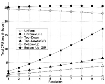
In Figure 6, the total computation times for each method and resolution for the whole data set are shown. The bottom-up algorithm is clearly slower than the top-down, because the tested resolutions were such that the computational effort required by the bottom-up algorithm was about 10 times that required by the top-down algorithm (without fine-tuning by GIR). The uniform approach is naturally fast. However, because of poor initial placement of the break points, the GIR has to be run for many iterations, which is computationally expensive.

The total computational costs for each method and resolution for the whole data set (CPU hours).
5.2.2. Comparison of the heuristic algorithms with the optimal solution
In the second experiment, heuristic algorithms were tested against the optimal solution. Even though for computational reasons, only the first 1000 samples of each signal could be used, the test was run in order to attain some evidence of the reliability of the heuristic algorithms. In this experiment the number of signals was 467, less than in the previous experiment. We had to drop out 22 more signals because they had so many fixed segments in their first 1000 points that it was not possible to run the test using all the different resolutions for the uniform algorithm.
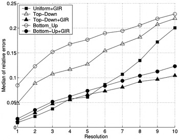
Figure 7 shows the medians of the relative errors over all signals for all methods and resolutions. For each signal, they were computed with Eq. (5) using the optimal result obtained by dynamical programming as the minimum.

The medians of the relative errors over all signals for different methods and resolutions. The results obtained by the uniform algorithm are significantly larger than all the others and are not shown.
Even though the best method in the previous experiment, the bottom-up algorithm (fine-tuned using GIR), was not the best one in any case, it performed steadily: it was always close to the best method at every resolution.
Another remarkable thing is that the absolute value of the median of the relative error between the optimal solution and the best heuristic algorithm is not large: depending on the resolution, it varies from about 0.01 to 0.1, which is 1–10%. In light of these results, the performance of the heuristic algorithms seems to be quite satisfactory.
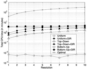
Finally, in Figure 8, the total computational costs for each method and resolution are shown. It is easy to see why the test was limited to 1000 first points of each signal only: the computation time for the optimal solution was about 300 min. Even for as few as 10,000 points, the time would have been approximately 200 days!

The total computational costs for each method and resolution (CPU minutes). Note that the scale of the vertical axis is logarithmic.
5.3. An example of process diagnostics
In this section, a brief example of an analysis described earlier (Section 4.1) is presented using all the same signals that were used in the tests above. The signals were preprocessed in a manner similar to that used in the previous experiment and modeled using a bottom-up algorithm fine-tuned using GIR, which was found to be the best among the different methods in the comparison using the full data set. The resolution was selected so that it corresponds to a 4-h run of the paper machine: the average number of samples in one segment was 24. The size of the original data set (which included all signals) was about 500 MB, which was dropped to about 65 MB in the modeling.
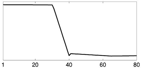
In phase 1, a query sequence (q0) of 80 points representing a level change in a signal of interest was extracted manually. This first query signal is shown in Figure 9.
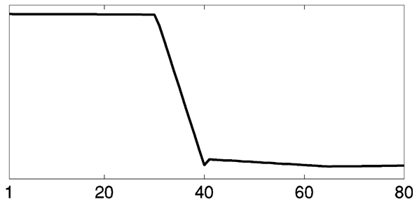
A query sequence that contains a (level) change of interest.
Next, in phase 2, similar changes were located in the same signal. Only changes on the same scale were the object of a search. Thus, the weights (w0, m) in Eq. (3) were all set to 1. After the search, the match vector (Q) consisted of M = 1057 sequences.
In phase 3, the query vector was pruned. An illustration of the pruning is shown in Figure 10. The first query sequence

with 24 best matches

are shown to the user. Of these, the three sequences

were considered as appropriate matches and selected for further inspection. Thus, the pruned query vector was

.

The pruning of the query vector. The first query sequence (“Query”) is shown in the top left corner. Among the 24 best matches, the analyst selects three sequences (marked with boxes) for further inspection.
In phase 4, we searched for the signals that were potentially responsible for the change. The value of dmin was set to −12 (i.e., 2 h) and dmax was set to 0. The distances between the query vector Q′ and match vectors of all the other 488 signals Si, i = 1,…, 488 were computed using Eq. (4).
An illustration of the query sequences and corresponding match sequences of a good match are shown in Figure 11. The delay that gave the best similarity was −2. That is, the change of interest occurs in the signal of interest two time instances after a change in the match signal.

An illustration of a good match to the query. The top row consists of the four query sequences, and the second row from the top shows the corresponding four match sequences. The bottom-left scatter plot shows the dependency revealed between the query and the match sequences. In the plot, all the points of the query vector are plotted against the points of the match vector. There is a clear linear dependency between the two. The bottom-right corner shows the same type of plot of the whole signal of interest versus all the points of the match signal. In the plot, the white box illustrates the region where the points of the query and the match vectors are located. The plot indicates that the local dependency revealed cannot be observed from all of the data.
6. SUMMARY AND CONCLUSIONS
This paper presents a detailed description of all the operations that are required in practice to build a piecewise linear model for a real signal. A novel preprocessing scheme that can be used to remove artifacts from process signals was suggested first. Then, a set of existing segmentation algorithms was reviewed and outlined; modifications required by the preprocessing to each algorithm were pointed out. In order to give an example of analysis methods where the piecewise linear models could be of benefit, a procedure for process diagnostics using subsequence matching was suggested.
A large experiment using real process data was carried out to find out which one of the heuristic piecewise linear modeling methods is best suited for the data at hand. Based on the results, it seems evident that if one should choose only one of the algorithms, it would be the bottom-up algorithm fine-tuned with GIR. However, if enough computational resources are available, running “a committee of segmentation algorithms” and choosing the best result is justified: no algorithm was totally superior to the others in all cases.
In the experiments, we also gave a simple example of process diagnostics procedure using real data in practice. It was demonstrated that the procedure is capable of detecting local dependencies in process measurement signals.
ACKNOWLEDGMENTS
I wish to thank Prof. Jaakko Hollmén and Lic. Sc. (Tech.) Jarmo Hurri for their valuable comments on the article.
APPENDIX A: FAST COMPUTATION OF MODEL ERROR AND LINE FIT
Error of an arbitrary segment s(t0, tf) is given by
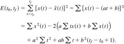
Minimization of E is straightforward: its partial derivatives with respect to unknown line fit parameters a and b are computed and set to zero and the equations are solved for a and b. After some calculus, the well-known least squares estimates are obtained:
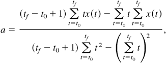
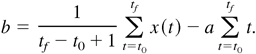
Fast computation of the model parameters [Eqs. (A2) and (A3)] and error [Eq. (A1)] is crucial. All these equations can be written in terms of partial sums of t, t2, x(t), tx(t), and x2(t) plus some operations that are independent of data. The partial sums can be computed for an arbitrary segment in constant time using the following cumulative sums:

In the formulas above, t = 1,…, N and cx(0) = cx2(0) = ctx(0) = ct(0) = ct2(0) = 0. Computation of each sum is a one-pass operation: it is linear in time and only needs to be done once. The memory requirement of each sum is N. For example, the error of each segment [Eq. (A1)] can be rewritten using the cumulative sums in the following way:
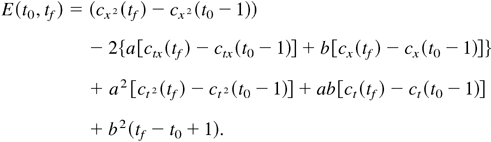
Also, the sums in Eqs. (A2) and (A3) can be rewritten in a similar manner. The operation is very straightforward and is therefore omitted here.
References
REFERENCES
Bakshi, B.R.
(1999).
Multiscale analysis and modeling using wavelets.
Journal of Chemometrics,
13(3–4),
415–434.Google Scholar
Bakshi, B.R. &
Stephanopoulos, G.
(1994).
Representation of process trends—III. A multiscale extraction
of trends from process data.
Computers and Chemical Engineering,
18(4),
267–302.Google Scholar
Basseville, M. &
Nikiforov, I.V.
(1993).
Detection of Abrupt Changes—Theory and Application.
Englewood Cliffs, NJ:
Prentice–Hall.
Available on-line at
http://www.irisa.fr/sigma2/kniga/.
Bellman, R.
(1961).
On the approximation of curves by line segments using dynamic
programming.
Communications of the ACM,
4(6),
284.Google Scholar
Bishop, C.M.
(1995).
Neural Networks for Pattern Recognition.
New York:
Oxford University Press.
Cantoni, A.
(1971).
Optimal curve fitting with piecewise linear functions.
IEEE Transactions on Computers,
C-20(1),
59–67.Google Scholar
Chen, B.H.,
Wang, X.Z.,
Yang, S.H., &
McGreavy, C.
(1999).
Application of wavelets and neural networks to diagnostic system
development, 1, Feature extraction.
Computers and Chemical Engineering,
23(7),
899–906.Google Scholar
Cheung, J.T.-Y. &
Stephanopoulos, G.
(1990).
Representation of process trends—part I. A formal
representation framework.
Computers and Chemical Engineering,
14(4/5),
495–510.Google Scholar
Chu, K.K.W. &
Wong, M.H.
(1999).
Fast time-series searching with scaling and shifting.
Proc. 18th ACM SIGMOD–SIGACT–SIGART Symp. on Principles
of Database Systems, pp.
237–248.
Djurić, P.M.
(1994).
A MAP solution to off-line segmentation of signals.
Proc. IEEE Int. Conf. Acoustics, Speech and Signal Processing,
Vol. 4, pp.
505–508.
Faloutsos, C.,
Ranganathan, M., &
Manolopoulus, Y.
(1994).
Fast subsequence matching in time-series databases.
Proc. 1994 ACM SIGMOD Int. Conf., pp.
419–429.
Guralnik, V. &
Srivastava, J.
(1999).
Event detection from time series data.
Proc. Fifth ACM SIGKDD Int. Conf. Knowledge Discovery and Data
Mining, pp.
33–42.
Hawkins, D.M.
(1976).
Point estimation of the parameters of piecewise regression models.
Applied Statistics,
25(1),
51–57.Google Scholar
Himberg, J.,
Korpiaho, K.,
Mannila, H.,
Tikanmäki, J., &
Toivonen, H.
(2001).
Time series segmentation for context recognition in mobile
devices.
Proc. 2001 IEEE Int. Conf. Data Mining, pp.
203–210.
Hyvärinen, A.
(1999).
Survey on independent component analysis.
Neural Computing Surveys,
2,
94–128.
Available on-line at
http://www.cse.ucsc.edu/NCS/.Google Scholar
Imai, H. &
Iri, M.
(1986).
An optimal algorithm for approximating a piecewise linear function.
Journal of Information Processing,
9(3),
159–162.Google Scholar
Keogh, E. &
Smyth, P.
(1997).
A probabilistic approach to fast pattern matching in time series
databases.
Proc. Third Int. Conf. Knowledge Discovery and Data Mining, pp.
24–30.
Konstantinides, K. &
Natarajan, B.K.
(1994).
An architecture for lossy compression of waveforms using
piecewise-linear approximation.
IEEE Transactions on Signal Processing,
42(9),
2449–2454.Google Scholar
Kourti, T. &
MacGregor, J.F.
(1995).
Process analysis, monitoring, and diagnosis using multivariate
projection methods.
Chemometrics & Intelligent Laboratory Systems,
28(1),
3–21.Google Scholar
Li, R.F. &
Wang, X.Z.
(2002).
Dimension reduction of process dynamic trends using independent
component analysis.
Computers and Chemical Engineering,
26(3),
467–473.Google Scholar
Love, P.L. &
Simaan, M.
(1988).
Automatic recognition of primitive changes in manufacturing process
signals.
Pattern Recognition,
4(21),
333–342.Google Scholar
McLeod, S.,
Nesic, Z.,
Davies, M.S.,
Dumont, G.A.,
Lee, F.,
Lofkrantz, E., &
Shaw, I.
(1998).
Paper machine data analysis and display using wavelet transforms.
IEEE Industry Applications 1998, Dynamic Modeling Control
Applications for Industry Workshop, pp.
59–62.
Nesic, Z.,
Davies, M., &
Dumont, G.
(1996).
Paper machine data compression using wavelets.
Proc. 1996 IEEE Int. Conf. Control Applications, pp.
161–166.
Nygaard, R.,
Melnikov, G., &
Katsaggelos, A.K.
(2001).
A rate distortion optimal ECG coding algorithm.
IEEE Transactions on Biomedical Engineering,
48(1),
28–40.Google Scholar
Oliver, J.J.,
Baxter, R.A., &
Wallace, C.S.
(1998).
Minimum message length segmentation.
Proc. Second Pacific-Asia Conf. Knowledge Discovery and Data
Mining, pp.
222–233.
Pavlidis, T.
(1973).
Waveform segmentation through functional approximation.
IEEE Transactions on Computers,
C-22(7),
689–697.Google Scholar
Pavlidis, T.
(1974).
Segmentation of plane curves.
IEEE Transactions on Computers,
C-23(8),
860–870.Google Scholar
Prandoni, P.,
Goodwin, M., &
Vetterli, M.
(1997).
Optimal time segmentation for signal modeling and compression.
Proc. 1997 IEEE Int. Conf. on Acoustics, Speech, and Signal
Processing,
Vol. 3, pp.
2029–2032.
Rengaswamy, R. &
Venkatasubramanian, V.
(1995).
A syntactic pattern-recognition approach for process monitoring and
fault diagnosis.
Engineering Applications of Artificial Intelligence,
8(1),
35–51.Google Scholar
The MathWorks, Inc.
(1999).
Using Matlab.
Natick, MA:
The MathWorks, Inc.
Vedam, H. &
Venkatasubramanian, V.
(1997).
A wavelet theory-based adaptive trend analysis system for process
monitoring and diagnosis.
Proc. American Control Conf., pp.
309–313.
Wang, X.Z.
(1999).
Data Mining and Knowledge Discovery for Process Monitoring and
Control.
London:
Springer.
Wu, L.-D.
(1984).
A piecewise linear approximation based on a statistical model.
IEEE Transactions on Pattern Analysis and Machine Intelligence,
PAMI-6(1),
41–45.CrossRefGoogle Scholar
Xiong, Z.,
Herley, C.,
Ramchandran, K., &
Orchard, M.T.
(1994).
Flexible time segmentations for time-varying wavelet packets.
Proc. IEEE-SP Int. Symp. on Time-Frequency and Time-Scale Analysis,
pp.
9–12.
Zhang, H.,
Tangirala, A.K., &
Shah, S.L.
(1999).
Dynamic process modeling using multiscale PCA.
Proc. 1999 IEEE Canadian Conf. Electrical and Computer Engineering,
pp.
1579–1584.
Phases 1–6 of the preprocessing from original (raw) data to preprocessed data.
The original signal (top) and the preprocessed signal (bottom) with corresponding old time labels on top and new time labels at the bottom. The two thick lines denote the fixed break points.
The six phases of the process diagnostics procedure. Phases 1, 3, and 5 require user interaction and are emphasized using a thick line.
Ten examples of the signals used in the experiments. Each plot contains 1000 points from one signal.
A comparison of the fast heuristic algorithms. Each plot is a histogram of relative errors that fall within the range [0, 1] for all signals using a fixed method at a fixed resolution. Note that in some cases a large part of the mass of the histogram is outside the plotted range [0, 1], because for some signals the relative error is >1. The numbers inside the graphs indicate the performance of the method at that resolution: the upper is the percentage of all signals for which the method was best, and the lower is the median of all relative errors in the histogram. At each resolution, the quantities of the best method are highlighted.
The total computational costs for each method and resolution for the whole data set (CPU hours).
The medians of the relative errors over all signals for different methods and resolutions. The results obtained by the uniform algorithm are significantly larger than all the others and are not shown.
The total computational costs for each method and resolution (CPU minutes). Note that the scale of the vertical axis is logarithmic.
A query sequence that contains a (level) change of interest.
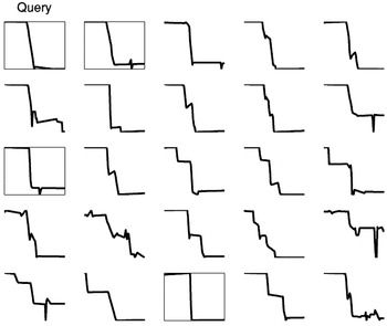
The pruning of the query vector. The first query sequence (“Query”) is shown in the top left corner. Among the 24 best matches, the analyst selects three sequences (marked with boxes) for further inspection.
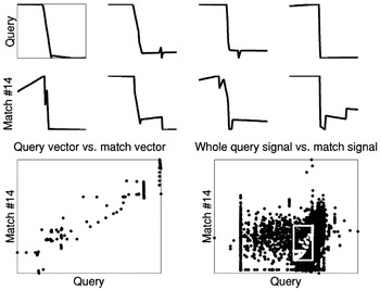
An illustration of a good match to the query. The top row consists of the four query sequences, and the second row from the top shows the corresponding four match sequences. The bottom-left scatter plot shows the dependency revealed between the query and the match sequences. In the plot, all the points of the query vector are plotted against the points of the match vector. There is a clear linear dependency between the two. The bottom-right corner shows the same type of plot of the whole signal of interest versus all the points of the match signal. In the plot, the white box illustrates the region where the points of the query and the match vectors are located. The plot indicates that the local dependency revealed cannot be observed from all of the data.
 You have
Access
- 1
- Cited by