2. Combined Evolutionary and Mass Modelling

To cover the full picture of a cluster’s evolution over time and its makeup today, we combine three different fast computational models, capturing different aspects of the cluster structure and evolution.

To model the evolution of the bulk properties of a cluster over the course of its lifetime, including the total mass, half-mass radius, and mass in BHs, we use the latest implementation of the clusterBH models, as described in Fronimos et al. (in prep).

Most free parameters of this model, which are shared across clusters, are set based on the calibration to a grid of CMC models. In our analysis, the initial mass and half-mass radius, as well as the slopes of the initial mass function (IMF) are allowed to vary freely. In order to model in more detail the present-day mass distributions of the clusters, such that they can be compared with a variety of observations, we use the limepy multimass distribution-function (DF) models (Gieles & Zocchi, Reference Gieles and Zocchi2015), through the GCfit Python package, as described in Dickson et al. (Reference Dickson, Hénault-Brunet and Baumgardt2023). The multimass version of these models, defined based on the sum of a number of component DFs for mass bins covering the range of stellar and remnant masses, allows us to account for and constrain the distribution of specific types of objects, like BHs, as they would arrange themselves within a system in equilibrium, like a GC. These models can then in turn be compared against a number of observable quantities, such as velocity dispersion, number density and mass function profiles.

In chaining these models together, the free parameters representing the initial conditions of the cluster are evolved through clusterBH to its current age, and these present-day values are then used as input to construct the multimass equilibrium DF model, alongside other free parameters representing aspects like the degree of velocity anisotropy or mass segregation. As clusterBH only solves for the bulk properties of the cluster, and we also require a description of the present-day mass function (PDMF) for the multimass models, we must also include a separate prescription which evolves the mass function from the IMF to the PDMF, accounting for stellar evolution, preferentially escaping stars and remnant formation. To handle this, we use the algorithm implemented in the SSPtools library, as described in Dickson et al. (Reference Dickson, Hénault-Brunet and Baumgardt2023), with the overall mass loss normalized to match the evolution described by clusterBH.

These coupled models provide us with an extremely fast pipeline for connecting the observations of clusters today with their initial conditions, and facilitate the full exploration of parameter space using Bayesian statistical sampling techniques.

3. Validation on Simulated Observations

We first test these new coupled models by fitting them to simulated observations from a large grid of CMC models in order to ensure that we are able to reproduce the evolution and initial conditions of realistic clusters. The mock observations were created from projected snapshots of the CMC models at around 13 Gyrs, and designed to mimic the quality and quantity of data that exists for most well-studied Milky Way GCs (Dickson et al., Reference Dickson, Smith and Hénault-Brunet2024).

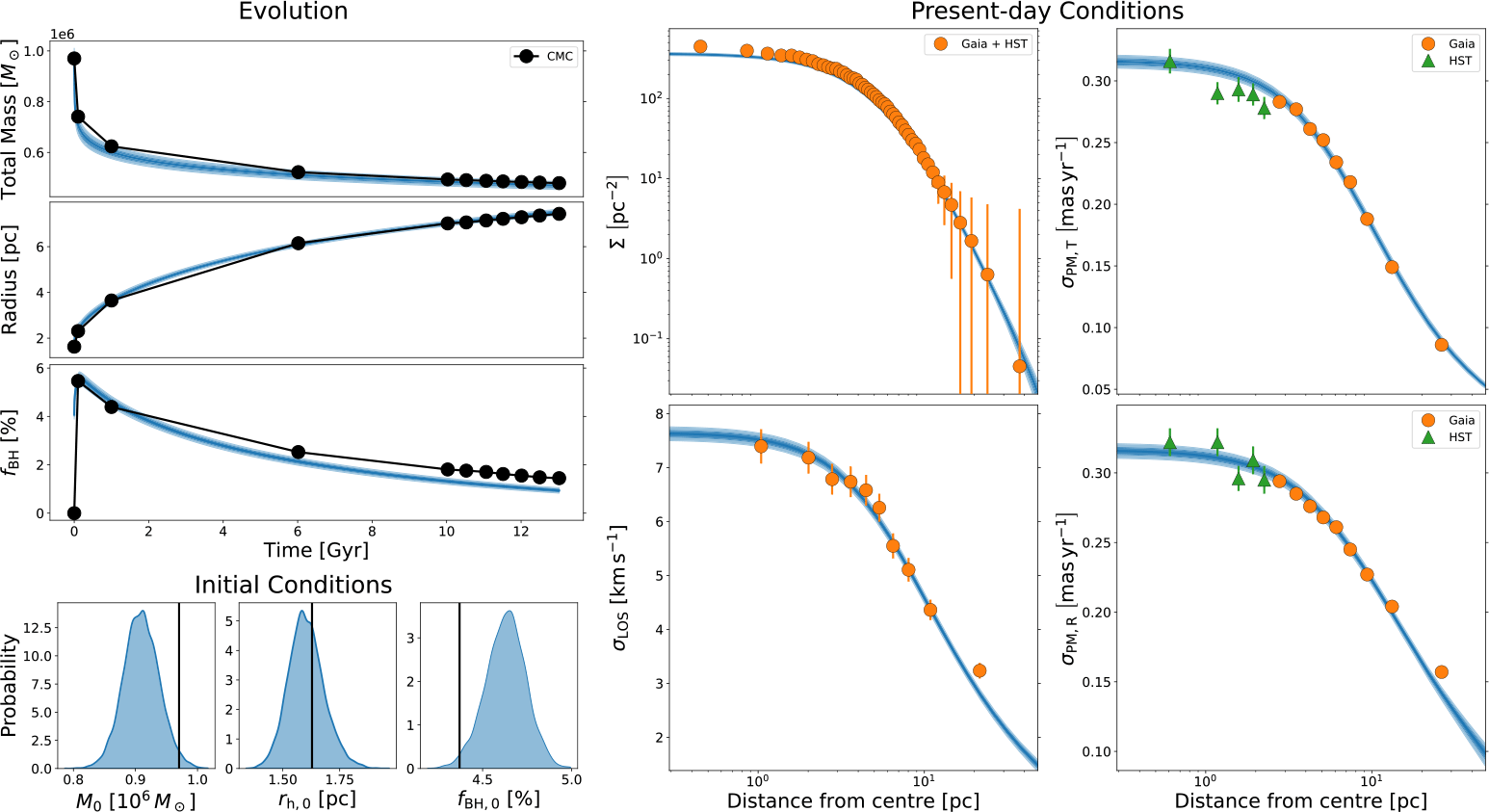
Figure 1 shows an example of the resulting fit of our models to these mock observational datasets. In the right panels, we can see that we are able to achieve remarkably good fits to the present-day data, while on the left we can see that, despite not being given any information outside of these mock observations, the models are able to recover both the evolution and initial conditions of the CMC models very well.

Figure 1.

Results of the model fit to the mock observations of the CMC model $N_0=1.6\times 10^6\ {M_{\odot}}$ , $r_{v,0}=2$ pc, $R_g=8$ kpc, $Z=0.002$ . Left: Evolution of the model total mass, half-mass radius and BH mass fraction over time (blue contours representing $1\sigma$ and $2\sigma$ credible intervals), and the full posterior distributions of the initial value of each. The “true” values from the CMC snapshots are shown in black. Right: Model radial profiles of surface number density ( $\Sigma$ ), line-of-sight velocity dispersions ( $\sigma_{\mathrm{LOS}}$ ), radial ( $\sigma_{\mathrm{PM},\mathrm{R}}$ ) and tangential ( $\sigma_{\mathrm{PM},\mathrm{T}}$ ) proper motion velocity dispersions. The mock observational datasets used to constrain the models are shown alongside their $1\sigma$ uncertainties by the orange and green points and error bars. The models are also fit to a number of fields of stellar mass functions at different projected distances from the cluster centre, not shown here, where similarly good agreement is found between model and observations.

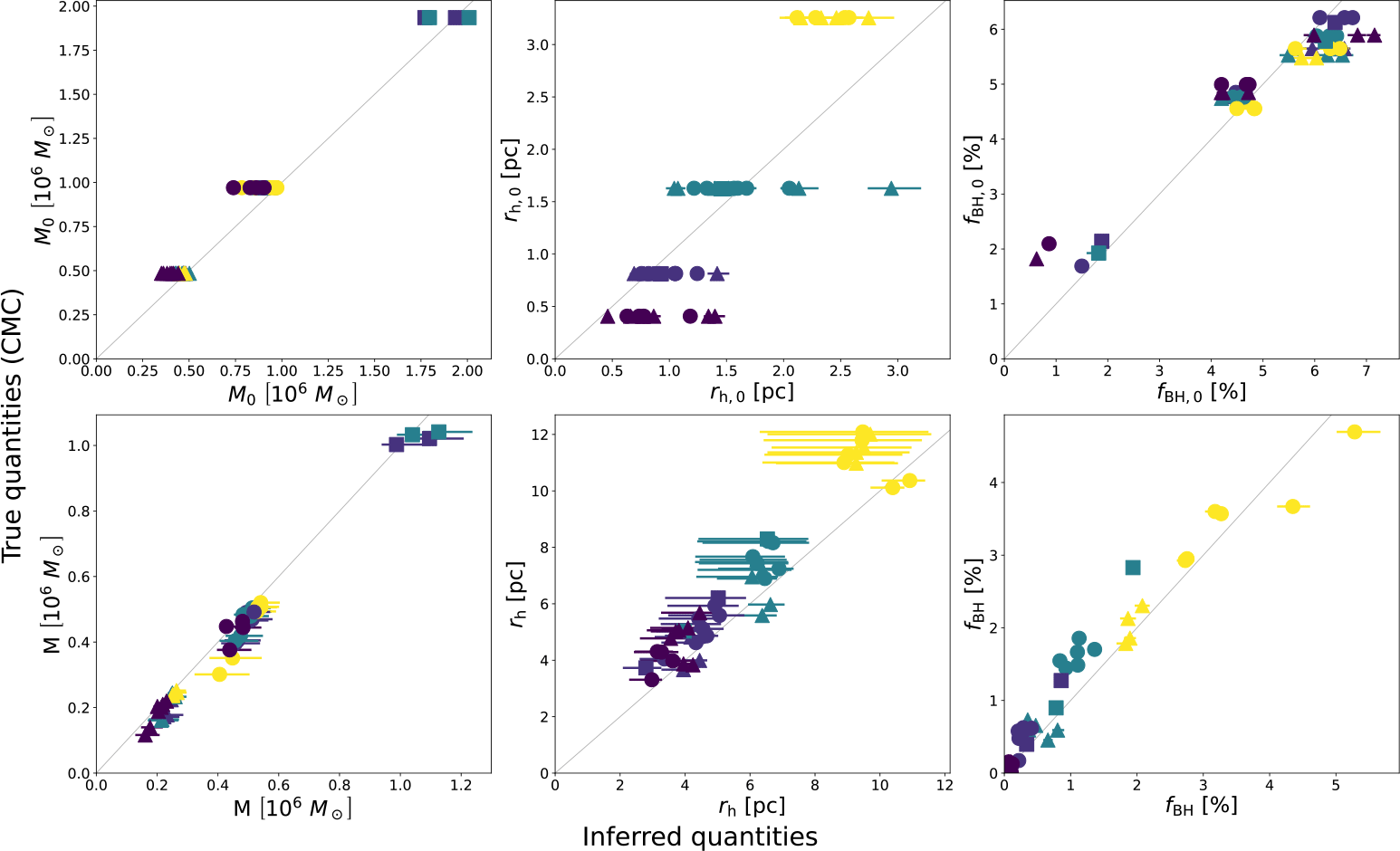
In Figure 2 we show the results of these fits and how well they are able to recover both the initial and final conditions, across all of the mock clusters in our validation sample. Apart from a few notable outliers, we are able to accurately infer both the initial and final quantities. A possible slight bias may appear in our fits of the largest ( $r_{v,0}=4$ pc) and smallest ( $r_{v,0}=0.5$ pc) initial radius mock clusters, where we tend to under- and overestimate the initial radius, respectively, though this is not entirely unexpected, as these models were not used to calibrate the clusterBH models in Fronimos et al. (in prep), and a corresponding bias is also shown and discussed in that paper.

Figure 2.

Resulting recovery of initial (top row) and present-day (bottom row) total mass, half-mass radius and BH mass fraction of all mock CMC cluster observations. The “true” values from the CMC models are shown on the y-axes, and our inferred values (and $1\sigma$ uncertainties) are shown on the x-axes. In each panel, the different initial masses in the CMC grid are denoted by marker shape, and different initial radii are denoted by colour.

4. Fitting on Real Clusters

We can next apply this fitting method to real GCs within the Milky Way. In this work, we turn to the same sample of clusters as in Dickson et al. (Reference Dickson, Hénault-Brunet and Baumgardt2023), which were selected based on their high quantity and quality of available kinematic and stellar mass function data, while spanning a range of metallicities. These fits demonstrate a good match between all of the model and present-day observations, similar to the mock tests.

When the evolution and initial conditions of these fits are examined, two notably interesting trends emerge. Firstly, the initial radii of the clusters are quite small (typically $r_{h,0}\lt 1.5$ pc), indicating that the clusters must begin their lives relatively dense. Secondly, the inferred IMF slopes of the clusters tend to favour more bottom-light IMFs than canonically assumed, more closely agreeing with the conclusions of Baumgardt et al. (Reference Baumgardt, Hénault-Brunet and Dickson2023).

5. Future Work

Extending this work to the full sample of nearby GCs will allow us to infer valuable information on the initial conditions of clusters within the Milky Way, and place further constraints on their populations of BHs, both in the past and retained to today.

The flexibility and speed of these models also allows us to easily change various components and assumptions and test their impacts. While in the above results we assumed the same BH physics as used in the CMC grid, a key component of this work will be to examine the effects of the initial population of BHs created and retained in the cluster, by experimenting with a variety of prescriptions for the supernovae natal kicks received by BHs. By comparing commonly assumed and flexible prescriptions, we can measure their relative likelihoods and attempt to place some constraints on this extremely uncertain process.

Together, the information learned through these fits will also inform analyses of larger samples of clusters, where the observational data may be lacking, and thus enable investigations of the initial conditions of the population of Milky Way GCs as a whole.