A model for confined vortex rings with elliptical-core vorticity distribution

Ionut Danaila; Felix Kaplanski; Sergei S. Sazhin

doi:10.1017/jfm.2016.752

A model for confined vortex rings with elliptical-core vorticity distribution

Published online by Cambridge University Press: 07 December 2016

Ionut Danaila,

Felix Kaplanski and

Sergei S. Sazhin

Show author details

Ionut Danaila: Affiliation:
Laboratoire de Mathématiques Raphaël Salem, Université de Rouen Normandie, F-76801 Saint-Étienne-du-Rouvray, France
Felix Kaplanski: Affiliation:
Tallinn University of Technology, Ehitajate tee 5, Tallinn 12616, EstoniaSir Harry Ricardo Laboratories, Advanced Engineering Centre, School of Computing, Engineering and Mathematics, University of Brighton, Brighton BN2 4GJ, UK
Sergei S. Sazhin*: Affiliation:
Sir Harry Ricardo Laboratories, Advanced Engineering Centre, School of Computing, Engineering and Mathematics, University of Brighton, Brighton BN2 4GJ, UK
*: †Email address for correspondence: S.Sazhin@brighton.ac.uk

Article contents

Abstract
Introduction
Background
Radially confined vortex rings with elliptical cores
Predictions of the model versus direct numerical simulations
An heuristic relation between vortex ring energy and circulation
Summary and discussion
References

Rights & Permissions

Abstract

We present a new model for an axisymmetric vortex ring confined in a tube. The model takes into account the elliptical (elongated) shape of the vortex ring core and thus extends our previous model (Danaila et al. J. Fluid Mech., vol. 774, 2015, pp. 267–297) derived for vortex rings with quasi-circular cores. The new model offers a more accurate description of the deformation of the vortex ring core, induced by the lateral wall, and a better approximation of the translational velocity of the vortex ring, compared with the previous model. The main ingredients of the model are the following: the description of the vorticity distribution in the vortex ring is based on the previous model of unconfined elliptical-core vortex rings (Kaplanski et al. Phys. Fluids, vol. 24, 2012, 033101); Brasseur’s approach (Brasseur, NASA Tech. Rep. JIAA TR-26, 1979) is then applied to derive a wall-induced correction for the Stokes streamfunction of the confined vortex ring flow. We derive closed formulae for the flow streamfunction and vorticity distributions. An asymptotic expression for the long-time evolution of the drift velocity of the vortex ring as a function of the ellipticity parameter is also derived. The predictions of the model are shown to be in agreement with direct numerical simulations of confined vortex rings generated by a piston–cylinder mechanism. The predictions of the model support the recently suggested heuristic relation (Krieg & Mohseni Trans. ASME J. Fluids Engng, vol. 135, 2013, 124501) between the energy and circulation of vortex rings with converging radial velocity. A new procedure for fitting experimental and numerical data with the predictions of the model is described. This opens the way for applying the model to realistic confined vortex rings in various applications including those in internal combustion engines.

JFM classification

Vortex Flows: Vortex dynamics Vortex Flows: Vortex Flows Vortex Flows: Vortex interactions

Information

Type: Papers
Information: Journal of Fluid Mechanics , Volume 811 , 25 January 2017, pp. 67 - 94
DOI: https://doi.org/10.1017/jfm.2016.752 [Opens in a new window]
Copyright: © 2016 Cambridge University Press

1 Introduction

A large amount of the physical and mathematical literature has been devoted to the study of vortex rings in unbounded domains (see the reviews by Shariff & Leonard (Reference Shariff and Leonard1992), Lim & Nickels (Reference Lim, Nickels and Green1995), Fukumoto (Reference Fukumoto2010)). The study of radially confined vortex ring flows has received far less attention, despite its importance in many practical applications. These include vortex ring-like structures in gasoline internal combustion engines (Begg et al. Reference Begg, Kaplanski, Sazhin, Hindle and Heikal2009) and transient flow fields behind arterial stenoses (Gharib et al. Reference Gharib, Rambod, Kheradvar, Sahn and Dabiri2006).

To the best of the authors’ knowledge, the first theoretical analysis of confined vortex rings was performed by Brasseur (Reference Brasseur1979). He assumed that the flow field in the outer region (far from the core) depends on its total circulation but not on the details of the ring’s vorticity distribution. The vortex ring in his study was represented as a thin circular vortex filament (CVF) (Lamb Reference Lamb1932), with given initial circulation $\unicode[STIX]{x1D6E4}_{0}$ and radius $R_{0}$ . Then the streamfunction of the confined vortex ring was decomposed as a sum of an unconfined streamfunction for the CVF and a correction streamfunction induced by the tube (Brasseur Reference Brasseur1986). Danaila, Kaplanski & Sazhin (Reference Danaila, Kaplanski and Sazhin2015) applied Brasseur’s method using not the CVF but a more realistic vorticity distribution in the vortex ring based on the unconfined viscous vortex ring model derived by Kaplanski & Rudi (Reference Kaplanski and Rudi1999, Reference Kaplanski and Rudi2005). The wall-induced correction of the streamfunction was derived analytically, giving closed analytical formulae for the vorticity and streamfunction of a confined vortex ring. Using the power-law assumption for the time variation of the viscous length of the vortex ring, the time variations of the main integral characteristics such as circulation, kinetic energy and translational velocity were obtained. The predictions of this model were shown to be in agreement with available experimental data (Stewart et al. Reference Stewart, Niebel, Jung and Vlachos2012) and results of direct numerical simulations.

The confined vortex ring model suggested by Danaila et al. (Reference Danaila, Kaplanski and Sazhin2015) is based on the assumption that the vorticity distribution of the vortex ring is a quasi-isotropic Gaussian. This assumption was inferred from the unconfined vortex ring model suggested by Kaplanski & Rudi (Reference Kaplanski and Rudi1999, Reference Kaplanski and Rudi2005). This model was analytically derived as a first-order solution of the linearised axisymmetric Navier–Stokes equation. The measurements of unconfined or confined vortex ring vorticity, however, show that the vorticity field of the vortex ring deforms during its development (Fukumoto & Moffatt Reference Fukumoto and Moffatt2000); at later stages it becomes elongated due to Reynolds number effects (Weigand & Gharib Reference Weigand and Gharib1997; Danaila & Helie Reference Danaila and Helie2008). This deformation is accompanied by the modification of the vorticity distribution function and leads to changes in vortex ring integral characteristics. For example, the compression of the vorticity during the formation stage leads to an increase in both ring translational velocity ( $U$ ) and the downstream distance at which the separation of the ring from the trailing jet occurs. At the decay stage, this leads to an enhanced reduction of the values of $U$ . Also, the deformation of the vortex ring core has been observed in the process of the ring interaction with other vortex structures, e.g. vortex ring interaction with a columnar vortex (Candon & Marshall Reference Candon and Marshall2012). It was shown that taking into account the effects of ellipticity leads to better predictions of the translational velocity of the vortex ring when compared to experimentally observed rings (Weigand & Gharib Reference Weigand and Gharib1997) or the predictions of previously developed vortex ring models (Fukumoto & Moffatt Reference Fukumoto and Moffatt2008).

For a vortex ring confined in a tube, the elongated shape of the vortex core is accentuated by the interaction with the lateral wall (Danaila et al. Reference Danaila, Kaplanski and Sazhin2015). Also, the tube wall induces the deformation of the streamlines of the flow, without significant changing of the vorticity field. Based on these observations, we have developed a new model for a confined vortex ring, taking into account the elliptic shape of the vortex core. As in the model suggested by Kaplanski, Fukumoto & Rudi (Reference Kaplanski, Fukumoto and Rudi2012), the ellipticity of the vorticity distribution in the vortex ring is taken into account. As in our earlier model (Danaila et al. Reference Danaila, Kaplanski and Sazhin2015) Brasseur’s method is used to take into account the streamfunction correction induced by the wall. In the new model, the elliptical distribution of vorticity is postulated, while other properties, such as circulation $\unicode[STIX]{x1D6E4}$ , kinetic energy $E$ , translational velocity $U$ and streamfunction $\unicode[STIX]{x1D6F9}$ , are calculated. The main motivation for using a more realistic elliptical description of the vorticity distribution in the vortex rings is to render the model useful for practical applications requiring an accurate but simple model for describing the geometry of confined vortex rings (e.g. vortex rings in gasoline internal combustion engines (Begg et al. Reference Begg, Kaplanski, Sazhin, Hindle and Heikal2009; Sazhin Reference Sazhin2014)) or for reconstructing the velocity field around a vortex ring when only incomplete measurements are available (see Zhang & Danaila Reference Zhang and Danaila2012; Danaila & Protas Reference Danaila and Protas2015).

The paper is organised as follows. Previously developed analytical vortex ring models taking into account the effects of the radial confinement and ellipticity of the vortex ring core are summarised in § 2. In § 3 a new model for the confined elliptical-core vortex ring is described. In § 4 direct numerical simulations of axisymmetric vortex rings are used to assess the applicability of the new model. The predictions of the new model are compared with the heuristic relation between vortex ring energy and circulation suggested by Krieg & Mohseni (Reference Krieg and Mohseni2013) in § 5. The main results of the paper are summarised in § 6.

2 Background

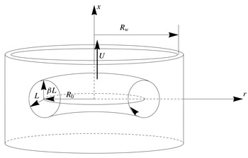
Danaila et al. (Reference Danaila, Kaplanski and Sazhin2015) considered an axisymmetric vortex ring of radius $R_{0}$ placed in an infinitely long rigid tube of radius $R_{w}$ , moving in an incompressible fluid with translational velocity $U$ along the axis of symmetry ( $x$ ) (see figure 1). For a given instant $t$ , the vorticity $\unicode[STIX]{x1D714}(r,x)$ and the Stokes streamfunction $\unicode[STIX]{x1D6F9}(r,x)$ are determined by the following equations (Batchelor Reference Batchelor1988):

(2.1a,b )

$$\begin{eqnarray}\displaystyle {\mathcal{L}}\unicode[STIX]{x1D6F9}=\unicode[STIX]{x1D714},\quad {\mathcal{L}}:=-\frac{\unicode[STIX]{x2202}}{\unicode[STIX]{x2202}r}\left(\frac{1}{r}\frac{\unicode[STIX]{x2202}}{\unicode[STIX]{x2202}r}\right)-\frac{\unicode[STIX]{x2202}}{\unicode[STIX]{x2202}x}\left(\frac{1}{r}\frac{\unicode[STIX]{x2202}}{\unicode[STIX]{x2202}x}\right)=-\frac{1}{r}\left(\frac{\unicode[STIX]{x2202}^{2}}{\unicode[STIX]{x2202}r^{2}}+\frac{\unicode[STIX]{x2202}^{2}}{\unicode[STIX]{x2202}x^{2}}-\frac{1}{r}\frac{\unicode[STIX]{x2202}}{\unicode[STIX]{x2202}r}\right),\hspace{24.0pt} & & \displaystyle\end{eqnarray}$$

where $x$ , $r$ are the axes of a cylindrical coordinate system. We consider the following boundary conditions: at the axis of symmetry,

(2.2)

$$\begin{eqnarray}\displaystyle \unicode[STIX]{x1D714}(0,x)=\unicode[STIX]{x1D6F9}(0,x)=0,\quad \text{for }r=0, & & \displaystyle\end{eqnarray}$$

vanishing vorticity and streamfunction in the far field,

(2.3)

$$\begin{eqnarray}\displaystyle \unicode[STIX]{x1D714},\unicode[STIX]{x1D6F9}\rightarrow 0\quad \text{when }(x^{2}+r^{2})^{1/2}\rightarrow \infty , & & \displaystyle\end{eqnarray}$$

and no flow through the tube wall,

(2.4a,b )

$$\begin{eqnarray}\displaystyle \unicode[STIX]{x1D714}\rightarrow 0,\quad \frac{1}{r}\frac{\unicode[STIX]{x2202}\unicode[STIX]{x1D6F9}}{\unicode[STIX]{x2202}x}=0,\quad \text{for }r=R_{w}. & & \displaystyle\end{eqnarray}$$

Brasseur (Reference Brasseur1979) represented the vortex ring as a circular vortex filament (CVF) and derived a correction of the streamfunction of the flow to satisfy the boundary condition (2.4) at the wall. Danaila et al. (Reference Danaila, Kaplanski and Sazhin2015) used an approach similar to that used by Brasseur (Reference Brasseur1979), but replaced CVF with the more realistic vortex ring model derived by Kaplanski & Rudi (Reference Kaplanski and Rudi1999, Reference Kaplanski and Rudi2005). This was possible since the vortex filament does not include any description of the vortex geometry. In what follows we summarise the main formulae used in the model developed by Danaila et al. (Reference Danaila, Kaplanski and Sazhin2015). This model is hereafter referred to as the vortex ring model with a circular core (VRC) and the subscript VRC will be used to identify the parameters obtained in this model.

Figure 1.

Schematic of a vortex ring in a tube. The elliptical core is described using two length scales: $L$ in the radial direction and $\unicode[STIX]{x1D6FD}L$ in the streamwise direction.

Danaila et al. (Reference Danaila, Kaplanski and Sazhin2015) scaled physical variables as:

(2.5a-d )

$$\begin{eqnarray}\displaystyle x_{1}=\frac{x-X_{0}}{R_{0}},\quad r_{1}=\frac{r}{R_{0}},\quad \unicode[STIX]{x1D714}^{\ast }=\frac{\unicode[STIX]{x1D714}R_{0}^{2}}{\unicode[STIX]{x1D6E4}_{0}},\quad \unicode[STIX]{x1D6F9}^{\ast }=\frac{\unicode[STIX]{x1D6F9}}{\unicode[STIX]{x1D6E4}_{0}R_{0}}, & & \displaystyle\end{eqnarray}$$

where $R_{0}$ is the radius of the vortex ring, $\unicode[STIX]{x1D6E4}_{0}$ its initial circulation and $X_{0}$ the streamwise position of the vortex centre. In what follows, the star superscripts are dropped and the vorticity and the streamfunction are considered as dimensionless. The vortex ring model derived by Kaplanski & Rudi (Reference Kaplanski and Rudi1999, Reference Kaplanski and Rudi2005) is described by parameter $\unicode[STIX]{x1D703}_{c}$ :

(2.6)

$$\begin{eqnarray}\displaystyle \unicode[STIX]{x1D703}_{c}=\frac{R_{0}}{L_{c}}, & & \displaystyle\end{eqnarray}$$

where $L_{c}$ is the diffusivity length (see figure 1), which is assumed to vary in time following a power law for laminar vortex rings:

(2.7)

$$\begin{eqnarray}\displaystyle \unicode[STIX]{x1D703}_{c}=\frac{R_{0}}{\sqrt{2\unicode[STIX]{x1D708}t}}, & & \displaystyle\end{eqnarray}$$

where $\unicode[STIX]{x1D708}$ is the fluid kinematic viscosity. The generalisation of (2.7) for turbulent vortex rings was discussed by Kaplanski et al. (Reference Kaplanski, Sazhin, Fukumoto, Begg and Heikal2009). The Reynolds number of the flow is introduced as $Re=\unicode[STIX]{x1D6E4}_{0}/\unicode[STIX]{x1D708}$ and the parameter $\unicode[STIX]{x1D700}=R_{0}/R_{w}<1$ quantifies the confinement of the vortex ring. The wall is located at $r_{1w}=1/\unicode[STIX]{x1D700}$ .

Following Brasseur’s approach, streamfunction $\unicode[STIX]{x1D6F9}^{w}$ describing the flow generated by a viscous vortex ring in a tube is presented as the sum of the streamfunction of the unbounded vortex ring $\unicode[STIX]{x1D6F9}$ and the wall-induced correction $-\unicode[STIX]{x1D6F9}^{0}$ . In the VRC model the streamfunction of the flow was presented as:

(2.8)

$$\begin{eqnarray}\displaystyle \unicode[STIX]{x1D6F9}_{VRC}^{w}(x_{1},r_{1})=\unicode[STIX]{x1D6F9}_{VRC}(x_{1},r_{1})-\unicode[STIX]{x1D6F9}_{VRC}^{0}(x_{1},r_{1}), & & \displaystyle\end{eqnarray}$$

where

(2.9)

$$\begin{eqnarray}\displaystyle \unicode[STIX]{x1D6F9}_{VRC} & = & \displaystyle \frac{r_{1}\unicode[STIX]{x1D703}_{c}}{4}\int _{0}^{\infty }\left[\exp (x_{1}\unicode[STIX]{x1D703}_{c}\unicode[STIX]{x1D707})\text{erfc}\left(\frac{\unicode[STIX]{x1D707}+x_{1}\unicode[STIX]{x1D703}_{c}}{\sqrt{2}}\right)+\exp (-x_{1}\unicode[STIX]{x1D703}_{c}\unicode[STIX]{x1D707})\text{erfc}\left(\frac{\unicode[STIX]{x1D707}-x_{1}\unicode[STIX]{x1D703}_{c}}{\sqrt{2}}\right)\right]\nonumber\\ \displaystyle & & \displaystyle \times \,\text{J}_{1}(r_{1}\unicode[STIX]{x1D703}_{c}\unicode[STIX]{x1D707})\text{J}_{1}(\unicode[STIX]{x1D703}_{c}\unicode[STIX]{x1D707})\,\text{d}\unicode[STIX]{x1D707}.\end{eqnarray}$$

Streamfunction $\unicode[STIX]{x1D6F9}_{VRC}$ corresponds to the vorticity distribution predicted by the unbounded vortex ring model derived by Kaplanski & Rudi (Reference Kaplanski and Rudi1999, Reference Kaplanski and Rudi2005):

(2.10)

$$\begin{eqnarray}\displaystyle \unicode[STIX]{x1D714}_{VRC}=\frac{\unicode[STIX]{x1D703}_{c}^{3}}{\sqrt{2\unicode[STIX]{x03C0}}}\exp \left(-\frac{(r_{1}^{2}+x_{1}^{2}+1)\unicode[STIX]{x1D703}_{c}^{2}}{2}\right)\text{I}_{1}\left(r_{1}\unicode[STIX]{x1D703}_{c}^{2}\right). & & \displaystyle\end{eqnarray}$$

In (2.9) and (2.10), $\text{J}_{1}$ is the Bessel function of the first kind, $\text{I}_{1}$ the modified Bessel function of the first kind and $\text{erfc}$ the complementary error function

(2.11)

$$\begin{eqnarray}\displaystyle \text{erfc}(x)=\frac{2}{\sqrt{\unicode[STIX]{x03C0}}}\int _{x}^{\infty }\exp (-t^{2})\,\text{d}t. & & \displaystyle\end{eqnarray}$$

Using series expansion in (2.9) in terms of $z_{1}=\unicode[STIX]{x1D703}_{c}\sqrt{x_{1}^{2}+r_{1}^{2}}\rightarrow \infty$ , it was shown that the limit of the streamfunction (2.9) at a large distance from the ring’s core is identical to that found by Brasseur (Reference Brasseur1979) for the circular vortex filament. The streamfunction correction $\unicode[STIX]{x1D6F9}_{VRC}^{0}$ induced by the presence of the tube was then found as:

(2.12)

$$\begin{eqnarray}\displaystyle \unicode[STIX]{x1D6F9}_{VRC}^{0}=\frac{r_{1}}{\unicode[STIX]{x03C0}}\int _{0}^{\infty }\frac{\text{K}_{1}(\unicode[STIX]{x1D707}/\unicode[STIX]{x1D700})}{\text{I}_{1}(\unicode[STIX]{x1D707}/\unicode[STIX]{x1D700})}\text{I}_{1}(\unicode[STIX]{x1D707})\text{I}_{1}(r_{1}\unicode[STIX]{x1D707})\cos (x_{1}\unicode[STIX]{x1D707})\,\text{d}\unicode[STIX]{x1D707}, & & \displaystyle\end{eqnarray}$$

where $\text{K}_{1}$ is the modified Bessel function of the second kind.

The streamfunction (2.8) along with the vorticity distribution (2.10) represent an approximate solution to problem (2.1) with boundary conditions (2.2)–(2.4). Using the power-law assumption (2.7), the time-dependent integral characteristics of the confined vortex ring flow based on the VRC model were predicted. When compared with those obtained by direct numerical simulations, a good agreement was obtained. The largest difference between analytical and numerical results was observed for relatively high Reynolds numbers, when the quasi-circular shape of the vortex core resulting from the vorticity distribution (2.10) turned out not to be very accurate. It is anticipated that the accuracy of a more advanced model taking into account realistic elliptical shapes of vortex ring cores, described in the next section, will improve the accuracy of the Danaila et al. (Reference Danaila, Kaplanski and Sazhin2015) model.

The confined vortex ring model taking into account the ellipticity of the vortex ring core, described later in § 3, is based on the model suggested by Kaplanski et al. (Reference Kaplanski, Fukumoto and Rudi2012) for an unbounded viscous vortex ring with an elliptical cross-section.

This model, hereafter referred to as the VRE model, is based on imposing weak perturbations on the first-order solution (2.10) for the vorticity in order to find an approximation of the nonlinear solution to the Navier–Stokes equations for high Reynolds numbers. Parameter $\unicode[STIX]{x1D6FD}$ (see figure 1) allowed Kaplanski et al. (Reference Kaplanski, Fukumoto and Rudi2012) to take into account the deformation of the vortex ring core along the streamwise direction. Using scaling (2.5), the non-dimensional vorticity for the VRE model was expressed as:

(2.13)

$$\begin{eqnarray}\displaystyle \unicode[STIX]{x1D714}_{VRE}=\frac{\unicode[STIX]{x1D703}_{e}^{3}}{\unicode[STIX]{x1D6FD}\sqrt{2\unicode[STIX]{x03C0}}}\exp \left(-\frac{(r_{1}^{2}+(x_{1}/\unicode[STIX]{x1D6FD})^{2}+1)\unicode[STIX]{x1D703}_{e}^{2}}{2}\right)\text{I}_{1}\left(r_{1}\unicode[STIX]{x1D703}_{e}^{2}\right), & & \displaystyle\end{eqnarray}$$

where

(2.14)

$$\begin{eqnarray}\displaystyle \unicode[STIX]{x1D703}_{e}=\frac{R_{0}}{L_{e}}=\unicode[STIX]{x1D706}\unicode[STIX]{x1D703}_{c}\Longrightarrow L_{e}=\frac{L_{c}}{\unicode[STIX]{x1D706}}, & & \displaystyle\end{eqnarray}$$

$L_{e}$ is the new viscous length scale.

Parameters $\unicode[STIX]{x1D6FD}>0$ and $\unicode[STIX]{x1D706}>0$ describe the elongation or compression along axes $x$ and $r$ , respectively, when compared to the VRC model for the vortex ring with circular cross-section. Furthermore, two small parameters $\unicode[STIX]{x1D716}_{0}$ and $\unicode[STIX]{x1D6FE}^{0}$ were introduced, such that

(2.15a,b )

$$\begin{eqnarray}\displaystyle \unicode[STIX]{x1D6FD}=1+\unicode[STIX]{x1D716}_{0},\quad \unicode[STIX]{x1D706}=1+\unicode[STIX]{x1D6FE}^{0}, & & \displaystyle\end{eqnarray}$$

where $0\leqslant \unicode[STIX]{x1D716}_{0}<1$ and $0\leqslant \unicode[STIX]{x1D6FE}^{0}<1$ .

The streamfunction corresponding to vorticity distribution (2.13) was derived in the form:

(2.16)

$$\begin{eqnarray}\displaystyle \unicode[STIX]{x1D6F9}_{VRE} & = & \displaystyle \frac{r_{1}\unicode[STIX]{x1D703}_{e}}{4}\int _{0}^{\infty }\exp \left((\unicode[STIX]{x1D6FD}^{2}-1)\frac{\unicode[STIX]{x1D707}^{2}}{2}\right)\left[\exp (\unicode[STIX]{x1D707}x_{1}\unicode[STIX]{x1D703}_{e})\text{erfc}\left(\frac{\unicode[STIX]{x1D707}\unicode[STIX]{x1D6FD}+x_{1}\unicode[STIX]{x1D703}_{e}/\unicode[STIX]{x1D6FD}}{\sqrt{2}}\right)\right.\nonumber\\ \displaystyle & & \displaystyle \left.+\,\exp (-\unicode[STIX]{x1D707}x_{1}\unicode[STIX]{x1D703}_{e})\text{erfc}\left(\frac{\unicode[STIX]{x1D707}\unicode[STIX]{x1D6FD}-x_{1}\unicode[STIX]{x1D703}_{e}/\unicode[STIX]{x1D6FD}}{\sqrt{2}}\right)\right]\text{J}_{1}\left(\unicode[STIX]{x1D703}_{e}\unicode[STIX]{x1D707}\right)\text{J}_{1}\left(r_{1}\unicode[STIX]{x1D703}_{e}\unicode[STIX]{x1D707}\right)\,\text{d}\unicode[STIX]{x1D707}.\end{eqnarray}$$

After the change of variables $\unicode[STIX]{x1D707}\unicode[STIX]{x1D703}_{e}\rightarrow \unicode[STIX]{x1D707}$ in the integrand, at large distances $z=\unicode[STIX]{x1D703}_{e}\sqrt{x_{1}^{2}+r_{1}^{2}}\rightarrow \infty$ the streamfunction (2.16) was approximated by:

(2.17)

$$\begin{eqnarray}\displaystyle \unicode[STIX]{x1D6F9}_{VRE}\approx \unicode[STIX]{x1D6F9}_{VRE}^{a}=\frac{r_{1}}{2}\int _{0}^{\infty }\exp \left((\unicode[STIX]{x1D6FD}^{2}-1)\frac{\unicode[STIX]{x1D707}^{2}}{2\unicode[STIX]{x1D703}_{e}^{2}}\right)\exp (-|x_{1}|\unicode[STIX]{x1D707})\text{J}_{1}(\unicode[STIX]{x1D707})\text{J}_{1}(r_{1}\unicode[STIX]{x1D707})\,\text{d}\unicode[STIX]{x1D707}. & & \displaystyle\end{eqnarray}$$

In the next section the previously developed models, described above, will be combined to investigate the radially confined vortex rings with elliptical cores.

3 Radially confined vortex rings with elliptical cores

Brasseur’s methodology is applied to derive the streamfunction of the flow generated in a tube by the viscous vortex ring with vorticity distribution (2.13). A new scaling, based on $R_{w}$ as length scale, is introduced:

(3.1a,b )

$$\begin{eqnarray}\displaystyle \tilde{x}=\frac{x}{R_{w}}=\unicode[STIX]{x1D700}x_{1},\quad \tilde{r}=\frac{r}{R_{w}}=\unicode[STIX]{x1D700}r_{1}, & & \displaystyle\end{eqnarray}$$

where $\unicode[STIX]{x1D700}=R_{0}/R_{w}$ was defined earlier. The total streamfunction of the flow is decomposed as:

(3.2)

$$\begin{eqnarray}\displaystyle \unicode[STIX]{x1D6F9}_{VRE}^{w}=\unicode[STIX]{x1D6F9}_{VRE}-\unicode[STIX]{x1D6F9}_{VRE}^{0}, & & \displaystyle\end{eqnarray}$$

where the correction $\unicode[STIX]{x1D6F9}_{VRE}^{0}$ satisfies the equation ${\mathcal{L}}\unicode[STIX]{x1D6F9}_{VRE}^{0}=0$ , with operator ${\mathcal{L}}$ defined in (2.1), and the following boundary conditions at the wall (cf. (2.4)):

(3.3)

$$\begin{eqnarray}\displaystyle \frac{1}{\tilde{r}}\frac{\unicode[STIX]{x2202}\unicode[STIX]{x1D6F9}_{VRE}^{0}}{\unicode[STIX]{x2202}\tilde{x}}=\frac{1}{\tilde{r}}\frac{\unicode[STIX]{x2202}\unicode[STIX]{x1D6F9}_{VRE}}{\unicode[STIX]{x2202}\tilde{x}},\quad \text{at }\tilde{r}=1. & & \displaystyle\end{eqnarray}$$

An equivalent formulation is obtained by introducing the flow potential $\unicode[STIX]{x1D6F7}$ linked with $\unicode[STIX]{x1D6F9}$ by the following equations, giving the two components of the velocity vector:

(3.4a,b )

$$\begin{eqnarray}\displaystyle v_{r}=\frac{\unicode[STIX]{x2202}\unicode[STIX]{x1D6F7}}{\unicode[STIX]{x2202}r}=-\frac{1}{r}\frac{\unicode[STIX]{x2202}\unicode[STIX]{x1D6F9}}{\unicode[STIX]{x2202}x},\quad v_{x}=\frac{\unicode[STIX]{x2202}\unicode[STIX]{x1D6F7}}{\unicode[STIX]{x2202}x}=\frac{1}{r}\frac{\unicode[STIX]{x2202}\unicode[STIX]{x1D6F9}}{\unicode[STIX]{x2202}r}. & & \displaystyle\end{eqnarray}$$

This allows us to present an alternative form of (3.2):

(3.5)

$$\begin{eqnarray}\displaystyle \unicode[STIX]{x1D6F7}_{VRE}^{w}=\unicode[STIX]{x1D6F7}_{VRE}-\unicode[STIX]{x1D6F7}_{VRE}^{0}, & & \displaystyle\end{eqnarray}$$

with the correction potential satisfying the Laplace equation:

(3.6)

$$\begin{eqnarray}\displaystyle \unicode[STIX]{x1D6FB}^{2}\unicode[STIX]{x1D6F7}_{VRE}^{0}=0, & & \displaystyle\end{eqnarray}$$

and the following boundary condition at the wall:

(3.7)

$$\begin{eqnarray}\displaystyle \frac{\unicode[STIX]{x2202}\unicode[STIX]{x1D6F7}_{VRE}^{0}}{\unicode[STIX]{x2202}\tilde{r}}=\frac{\unicode[STIX]{x2202}\unicode[STIX]{x1D6F7}_{VRE}}{\unicode[STIX]{x2202}\tilde{r}},\quad \text{at }\tilde{r}=1. & & \displaystyle\end{eqnarray}$$

To derive an approximation of $\unicode[STIX]{x1D6F7}_{VRE}^{0}$ we assume that approximation (2.17) is valid in the vicinity of the wall. The non-dimensional potential (scaled by $\unicode[STIX]{x1D6E4}_{0}$ ) corresponding to the streamfunction (2.17) is obtained in the form:

(3.8)

$$\begin{eqnarray}\displaystyle \unicode[STIX]{x1D6F7}_{VRE}^{a}=-\frac{1}{2}\int _{0}^{\infty }\exp \left((\unicode[STIX]{x1D6FD}^{2}-1)\frac{\unicode[STIX]{x1D707}^{2}}{2\unicode[STIX]{x1D703}_{e}^{2}}\right)\exp (-|\tilde{x_{1}}|\unicode[STIX]{x1D707})\text{J}_{1}(\unicode[STIX]{x1D707})\text{J}_{0}(r_{1}\unicode[STIX]{x1D707})\,\text{d}\unicode[STIX]{x1D707}. & & \displaystyle\end{eqnarray}$$

This equation is rewritten in $(\tilde{r},\tilde{x})$ coordinates as:

(3.9)

$$\begin{eqnarray}\displaystyle \unicode[STIX]{x1D6F7}_{VRE}^{a}=-\frac{\unicode[STIX]{x1D700}}{2}\int _{0}^{\infty }\exp \left((\unicode[STIX]{x1D6FD}^{2}-1)\frac{\unicode[STIX]{x1D700}^{2}\unicode[STIX]{x1D707}^{2}}{2\unicode[STIX]{x1D703}_{e}^{2}}\right)\exp (-|\tilde{x}|\unicode[STIX]{x1D707})\text{J}_{1}(\unicode[STIX]{x1D700}\unicode[STIX]{x1D707})\text{J}_{0}(\tilde{r}\unicode[STIX]{x1D707})\,\text{d}\unicode[STIX]{x1D707}. & & \displaystyle\end{eqnarray}$$

Since $\unicode[STIX]{x1D6FD}=1+\unicode[STIX]{x1D716}_{0}$ (see (2.15)), we can use the following power series expansion in terms of the small parameter $\unicode[STIX]{x1D716}_{0}$ :

(3.10)

$$\begin{eqnarray}\displaystyle \exp \left((\unicode[STIX]{x1D6FD}^{2}-1)\frac{\unicode[STIX]{x1D700}^{2}\unicode[STIX]{x1D707}^{2}}{2\unicode[STIX]{x1D703}_{e}^{2}}\right) & = & \displaystyle \exp \left((2\unicode[STIX]{x1D716}_{0}+\unicode[STIX]{x1D716}_{0}^{2})\frac{\unicode[STIX]{x1D712}^{2}\unicode[STIX]{x1D707}^{2}}{2}\right)\nonumber\\ \displaystyle & = & \displaystyle 1+\unicode[STIX]{x1D716}_{0}\unicode[STIX]{x1D712}^{2}\unicode[STIX]{x1D707}^{2}+\frac{1}{2}\unicode[STIX]{x1D716}_{0}^{2}\unicode[STIX]{x1D712}^{2}\unicode[STIX]{x1D707}^{2}(1+\unicode[STIX]{x1D712}^{2}\unicode[STIX]{x1D707}^{2})+\cdots \,,\end{eqnarray}$$

where

(3.11)

$$\begin{eqnarray}\displaystyle \unicode[STIX]{x1D712}=\frac{\unicode[STIX]{x1D700}}{\unicode[STIX]{x1D703}_{e}}=\frac{L_{e}}{R_{w}} & & \displaystyle\end{eqnarray}$$

represents the ratio between the viscous length scale and the radius of the tube ( $\unicode[STIX]{x1D712}\,\ll \,1$ ).

Using the expansion

(3.12)

$$\begin{eqnarray}\displaystyle \text{J}_{1}(\unicode[STIX]{x1D700}\unicode[STIX]{x1D707})=\frac{\unicode[STIX]{x1D700}\unicode[STIX]{x1D707}}{2}-\frac{(\unicode[STIX]{x1D700}\unicode[STIX]{x1D707})^{3}}{16}+\frac{(\unicode[STIX]{x1D700}\unicode[STIX]{x1D707})^{5}}{384}+\cdots \,, & & \displaystyle\end{eqnarray}$$

and remembering that

(3.13)

$$\begin{eqnarray}\displaystyle \frac{\unicode[STIX]{x2202}^{n}}{\unicode[STIX]{x2202}x^{n}}\exp (-\unicode[STIX]{x1D707}x)=(-\unicode[STIX]{x1D707})^{n}\exp (-\unicode[STIX]{x1D707}x) & & \displaystyle\end{eqnarray}$$

potential (3.9) can be expanded as:

(3.14)

$$\begin{eqnarray}\displaystyle \unicode[STIX]{x1D6F7}_{VRE}^{a}=\frac{\unicode[STIX]{x1D700}}{2}\left(\frac{\unicode[STIX]{x1D700}}{2}\frac{\unicode[STIX]{x2202}S}{\unicode[STIX]{x2202}\tilde{x}}-\frac{\unicode[STIX]{x1D700}^{3}}{16}\frac{\unicode[STIX]{x2202}^{3}S}{\unicode[STIX]{x2202}\tilde{x}^{3}}+\frac{\unicode[STIX]{x1D700}^{5}}{384}\frac{\unicode[STIX]{x2202}^{5}S}{\unicode[STIX]{x2202}\tilde{x}^{5}}-\cdots \!\right), & & \displaystyle\end{eqnarray}$$

where

(3.15)

$$\begin{eqnarray}\displaystyle S=\int _{0}^{\infty }\left(1+\unicode[STIX]{x1D716}_{0}\unicode[STIX]{x1D712}^{2}\unicode[STIX]{x1D707}^{2}+\frac{1}{2}\unicode[STIX]{x1D716}_{0}^{2}\unicode[STIX]{x1D712}^{2}\unicode[STIX]{x1D707}^{2}(1+\unicode[STIX]{x1D712}^{2}\unicode[STIX]{x1D707}^{2})\right)\exp (-|\tilde{x}|\unicode[STIX]{x1D707})\text{J}_{0}(\tilde{r}\unicode[STIX]{x1D707})\,\text{d}\unicode[STIX]{x1D707}. & & \displaystyle\end{eqnarray}$$

Note that we kept an approximation of the order of $o(\unicode[STIX]{x1D716}_{0}^{2})$ . This approach can be extended to higher-order approximations in $\unicode[STIX]{x1D716}_{0}$ . From (3.14) and (3.15) it can be seen that the behaviour of potential $\unicode[STIX]{x1D6F7}_{VRE}^{a}$ at large distances is controlled by $S$ ; for $\unicode[STIX]{x1D716}_{0}=0$ the first harmonic of (3.14) represents a point dipole (although, in fact, a similar dependence of this potential on $\tilde{x}$ and $\tilde{r}$ takes place for any $\unicode[STIX]{x1D716}_{0}$ ).

The basic idea behind Brasseur’s method is that expansion (3.14) can be applied to the total flow field $\unicode[STIX]{x1D6F7}_{VRE}^{w}$ . In this case, function $S$ is replaced by function $Q=S-Q_{1}$ which satisfies the boundary condition of no flow through the tube wall ( $\unicode[STIX]{x2202}Q/\unicode[STIX]{x2202}\tilde{r}=0$ ) at $\tilde{r}=1$ . Following decomposition (3.5), function $Q_{1}$ is finally used to derive the correction potential as:

(3.16)

$$\begin{eqnarray}\displaystyle \unicode[STIX]{x1D6F7}_{VRE}^{0}=\frac{\unicode[STIX]{x1D700}}{2}\left(\frac{\unicode[STIX]{x1D700}}{2}\frac{\unicode[STIX]{x2202}Q_{1}}{\unicode[STIX]{x2202}\tilde{x}}-\frac{\unicode[STIX]{x1D700}^{3}}{16}\frac{\unicode[STIX]{x2202}^{3}Q_{1}}{\unicode[STIX]{x2202}\tilde{x}^{3}}+\frac{\unicode[STIX]{x1D700}^{5}}{384}\frac{\unicode[STIX]{x2202}^{5}Q_{1}}{\unicode[STIX]{x2202}\tilde{x}^{5}}-\cdots \!\right). & & \displaystyle\end{eqnarray}$$

Let us now rewrite (3.15) as:

(3.17)

$$\begin{eqnarray}\displaystyle S=D_{1}+(\unicode[STIX]{x1D716}_{0}\unicode[STIX]{x1D712}^{2}+{\textstyle \frac{1}{2}}\unicode[STIX]{x1D716}_{0}^{2}\unicode[STIX]{x1D712}^{2})D_{2}+{\textstyle \frac{1}{2}}\unicode[STIX]{x1D716}_{0}^{2}\unicode[STIX]{x1D712}^{4}D_{3}, & & \displaystyle\end{eqnarray}$$

where

(3.18)

$$\begin{eqnarray}\displaystyle & \displaystyle D_{1}=\int _{0}^{\infty }\exp (-|\tilde{x}|\unicode[STIX]{x1D707})\text{J}_{0}(\tilde{r}\unicode[STIX]{x1D707})\,\text{d}\unicode[STIX]{x1D707}=\frac{1}{\sqrt{(\tilde{x}^{2}+\tilde{r}^{2})}}=\frac{2}{\unicode[STIX]{x03C0}}\int _{0}^{\infty }\text{K}_{0}(\tilde{r}\unicode[STIX]{x1D707})\cos (\unicode[STIX]{x1D707}\tilde{x})\,\text{d}\unicode[STIX]{x1D707},\qquad & \displaystyle\end{eqnarray}$$

(3.19)

$$\begin{eqnarray}\displaystyle D_{2} & = & \displaystyle \int _{0}^{\infty }\unicode[STIX]{x1D707}^{2}\exp (-|\tilde{x}|\unicode[STIX]{x1D707})\text{J}_{0}(\tilde{r}\unicode[STIX]{x1D707})\,\text{d}\unicode[STIX]{x1D707}=\frac{(-\tilde{r}^{2}+2\tilde{x}^{2})}{(\tilde{x}^{2}+\tilde{r}^{2})^{5/2}}\nonumber\\ \displaystyle & = & \displaystyle -\frac{2}{\unicode[STIX]{x03C0}}\int _{0}^{\infty }\unicode[STIX]{x1D707}^{2}\text{K}_{0}(\tilde{r}\unicode[STIX]{x1D707})\cos (\unicode[STIX]{x1D707}\tilde{x})\,\text{d}\unicode[STIX]{x1D707},\end{eqnarray}$$

(3.20)

$$\begin{eqnarray}\displaystyle D_{3} & = & \displaystyle \int _{0}^{\infty }\unicode[STIX]{x1D707}^{4}\exp (-|\tilde{x}|\unicode[STIX]{x1D707})\text{J}_{0}(\tilde{r}\unicode[STIX]{x1D707})\,\text{d}\unicode[STIX]{x1D707}=\frac{3(3\tilde{r}^{4}-24\tilde{r}^{2}\tilde{x}^{2}+8\tilde{x}^{4})}{(\tilde{x}^{2}+\tilde{r}^{2})^{9/2}}\nonumber\\ \displaystyle & = & \displaystyle \frac{2}{\unicode[STIX]{x03C0}}\int _{0}^{\infty }\unicode[STIX]{x1D707}^{4}\text{K}_{0}(\tilde{r}\unicode[STIX]{x1D707})\cos (\unicode[STIX]{x1D707}\tilde{x})\,\text{d}\unicode[STIX]{x1D707}.\end{eqnarray}$$

Function $Q$ is sought in the following form:

(3.21)

$$\begin{eqnarray}\displaystyle Q & = & \displaystyle \left[D_{1}+\int _{0}^{\infty }f_{1}(\unicode[STIX]{x1D707})\text{I}_{0}(\tilde{r}\unicode[STIX]{x1D707})\cos (\unicode[STIX]{x1D707}\tilde{x})\,\text{d}\unicode[STIX]{x1D707}\right]\nonumber\\ \displaystyle & & \displaystyle +\,\left[\left(\unicode[STIX]{x1D716}_{0}\unicode[STIX]{x1D712}^{2}+\frac{1}{2}\unicode[STIX]{x1D716}_{0}^{2}\unicode[STIX]{x1D712}^{2}\right)D_{2}+\int _{0}^{\infty }f_{2}(\unicode[STIX]{x1D707})\unicode[STIX]{x1D707}^{2}\text{I}_{0}(\tilde{r}\unicode[STIX]{x1D707})\cos (\unicode[STIX]{x1D707}\tilde{x})\,\text{d}\unicode[STIX]{x1D707}\right]\nonumber\\ \displaystyle & & \displaystyle +\,\left[\frac{1}{2}\unicode[STIX]{x1D716}_{0}^{2}\unicode[STIX]{x1D712}^{4}D_{3}+\int _{0}^{\infty }f_{3}(\unicode[STIX]{x1D707})\unicode[STIX]{x1D707}^{4}\text{I}_{0}(\tilde{r}\unicode[STIX]{x1D707})\cos (\unicode[STIX]{x1D707}\tilde{x})\,\text{d}\unicode[STIX]{x1D707}\right].\end{eqnarray}$$

Remembering the definitions of integrals $D_{1}$ , $D_{2}$ and $D_{3}$ , this expression can be rewritten as:

(3.22)

$$\begin{eqnarray}\displaystyle Q & = & \displaystyle \int _{0}^{\infty }\left[\frac{2}{\unicode[STIX]{x03C0}}\text{K}_{0}(\tilde{r}\unicode[STIX]{x1D707})+f_{1}(\unicode[STIX]{x1D707})\text{I}_{0}(\tilde{r}\unicode[STIX]{x1D707})\right]\cos (\unicode[STIX]{x1D707}\tilde{x})\,\text{d}\unicode[STIX]{x1D707}\nonumber\\ \displaystyle & & \displaystyle +\,\int _{0}^{\infty }\left[\left(\unicode[STIX]{x1D716}_{0}\unicode[STIX]{x1D712}^{2}+\frac{1}{2}\unicode[STIX]{x1D716}_{0}^{2}\unicode[STIX]{x1D712}^{2}\right)\left(-\frac{2}{\unicode[STIX]{x03C0}}\right)\text{K}_{0}(\tilde{r}\unicode[STIX]{x1D707})+f_{2}(\unicode[STIX]{x1D707})\text{I}_{0}(\tilde{r}\unicode[STIX]{x1D707})\right]\unicode[STIX]{x1D707}^{2}\cos (\unicode[STIX]{x1D707}\tilde{x})\,\text{d}\unicode[STIX]{x1D707}\nonumber\\ \displaystyle & & \displaystyle +\,\int _{0}^{\infty }\left[\frac{1}{2}\unicode[STIX]{x1D716}_{0}^{2}\unicode[STIX]{x1D712}^{4}\left(\frac{2}{\unicode[STIX]{x03C0}}\right)\text{K}_{0}(\tilde{r}\unicode[STIX]{x1D707})+f_{3}(\unicode[STIX]{x1D707})\text{I}_{0}(\tilde{r}\unicode[STIX]{x1D707})\right]\unicode[STIX]{x1D707}^{4}\cos (\unicode[STIX]{x1D707}\tilde{x})\,\text{d}\unicode[STIX]{x1D707}.\end{eqnarray}$$

The boundary condition $\unicode[STIX]{x2202}Q/\unicode[STIX]{x2202}\tilde{r}=0$ at $\tilde{r}=1$ requires that

(3.23)

$$\begin{eqnarray}\displaystyle & \displaystyle f_{1}(\unicode[STIX]{x1D707})=\frac{2}{\unicode[STIX]{x03C0}}\frac{\text{K}_{1}(\unicode[STIX]{x1D707})}{\text{I}_{1}(\unicode[STIX]{x1D707})}, & \displaystyle\end{eqnarray}$$

(3.24)

$$\begin{eqnarray}\displaystyle & \displaystyle f_{2}(\unicode[STIX]{x1D707})=\left(\unicode[STIX]{x1D716}_{0}\unicode[STIX]{x1D712}^{2}+\frac{1}{2}\unicode[STIX]{x1D716}_{0}^{2}\unicode[STIX]{x1D712}^{2}\right)\left(-\frac{2}{\unicode[STIX]{x03C0}}\right)\frac{\text{K}_{1}(\unicode[STIX]{x1D707})}{\text{I}_{1}(\unicode[STIX]{x1D707})}, & \displaystyle\end{eqnarray}$$

(3.25)

$$\begin{eqnarray}\displaystyle & \displaystyle f_{3}(\unicode[STIX]{x1D707})=\frac{1}{2}\unicode[STIX]{x1D716}_{0}^{2}\unicode[STIX]{x1D712}^{4}\left(\frac{2}{\unicode[STIX]{x03C0}}\right)\frac{\text{K}_{1}(\unicode[STIX]{x1D707})}{\text{I}_{1}(\unicode[STIX]{x1D707})}. & \displaystyle\end{eqnarray}$$

Using these expressions for $f_{1}$ , $f_{2}$ and $f_{3}$ and (3.21), we obtain the new expression for function $Q=S-Q_{1}$ , with:

(3.26)

$$\begin{eqnarray}Q_{1}=-\frac{2}{\unicode[STIX]{x03C0}}\int _{0}^{\infty }\left[1-\left(\unicode[STIX]{x1D716}_{0}\unicode[STIX]{x1D712}^{2}+\frac{1}{2}\unicode[STIX]{x1D716}_{0}^{2}\unicode[STIX]{x1D712}^{2}\right)\unicode[STIX]{x1D707}^{2}+\frac{1}{2}\unicode[STIX]{x1D716}_{0}^{2}\unicode[STIX]{x1D712}^{4}\unicode[STIX]{x1D707}^{4}\right]\frac{\text{K}_{1}(\unicode[STIX]{x1D707})}{\text{I}_{1}(\unicode[STIX]{x1D707})}\text{I}_{0}(\tilde{r}\unicode[STIX]{x1D707})\cos (\unicode[STIX]{x1D707}\tilde{x})\,\text{d}\unicode[STIX]{x1D707}.\end{eqnarray}$$

Substituting this expression for $Q_{1}$ into (3.16), we obtain, after differentiation, the following expression:

(3.27)

$$\begin{eqnarray}\displaystyle \unicode[STIX]{x1D6F7}_{VRE}^{0} & = & \displaystyle \frac{\unicode[STIX]{x1D700}}{\unicode[STIX]{x03C0}}\int _{0}^{\infty }\left[\frac{\unicode[STIX]{x1D700}\unicode[STIX]{x1D707}}{2}+\frac{\unicode[STIX]{x1D700}^{3}\unicode[STIX]{x1D707}^{3}}{16}+\frac{\unicode[STIX]{x1D700}^{5}\unicode[STIX]{x1D707}^{5}}{384}\right]\nonumber\\ \displaystyle & & \displaystyle \times \,\left[1-\left(\unicode[STIX]{x1D716}_{0}+\frac{1}{2}\unicode[STIX]{x1D716}_{0}^{2}\right)\unicode[STIX]{x1D712}^{2}\unicode[STIX]{x1D707}^{2}+\frac{1}{2}\unicode[STIX]{x1D716}_{0}^{2}\unicode[STIX]{x1D712}^{4}\unicode[STIX]{x1D707}^{4}\right]\frac{\text{K}_{1}(\unicode[STIX]{x1D707})}{\text{I}_{1}(\unicode[STIX]{x1D707})}\text{I}_{0}(\tilde{r}\unicode[STIX]{x1D707})\sin (\unicode[STIX]{x1D707}\tilde{x})\,\text{d}\unicode[STIX]{x1D707}.\end{eqnarray}$$

Keeping in mind that the expression in the first brackets represents the expansion of $\text{I}_{1}(\unicode[STIX]{x1D700}\unicode[STIX]{x1D707})$ , we can present the potential field induced by the presence of the tube as:

(3.28)

$$\begin{eqnarray}\unicode[STIX]{x1D6F7}_{VRE}^{0}=\frac{\unicode[STIX]{x1D700}}{\unicode[STIX]{x03C0}}\int _{0}^{\infty }\left[1-\left(\unicode[STIX]{x1D716}_{0}+\frac{1}{2}\unicode[STIX]{x1D716}_{0}^{2}\right)\unicode[STIX]{x1D712}^{2}\unicode[STIX]{x1D707}^{2}+\frac{1}{2}\unicode[STIX]{x1D716}_{0}^{2}\unicode[STIX]{x1D712}^{4}\unicode[STIX]{x1D707}^{4}\right]\frac{\text{K}_{1}(\unicode[STIX]{x1D707})}{\text{I}_{1}(\unicode[STIX]{x1D707})}\text{I}_{0}(\tilde{r}\unicode[STIX]{x1D707})\text{I}_{1}(\unicode[STIX]{x1D700}\unicode[STIX]{x1D707})\sin (\unicode[STIX]{x1D707}\tilde{x})\,\text{d}\unicode[STIX]{x1D707}.\end{eqnarray}$$

Note that the terms in the square brackets represent the first terms in the series expansion of $\exp (-(\unicode[STIX]{x1D6FD}^{2}-1)(\unicode[STIX]{x1D712}^{2}\unicode[STIX]{x1D707}^{2})/2)$ . If we go back to (3.10) and keep the higher-order terms, we obtain in (3.17) only integrals depending on even powers of $\unicode[STIX]{x1D707}$ . These integrals have the following structure:

(3.29)

$$\begin{eqnarray}\displaystyle D_{2p}=\int _{0}^{\infty }\unicode[STIX]{x1D707}^{2p}\exp (-|\tilde{x}|\unicode[STIX]{x1D707})\text{J}_{0}(\tilde{r}\unicode[STIX]{x1D707})\,\text{d}\unicode[STIX]{x1D707}. & & \displaystyle\end{eqnarray}$$

It can be proven that (see appendix A):

(3.30)

$$\begin{eqnarray}\displaystyle D_{2p}=\frac{2(-1)^{p}}{\unicode[STIX]{x03C0}}\int _{0}^{\infty }\unicode[STIX]{x1D707}^{2p}\text{K}_{0}(\tilde{r}\unicode[STIX]{x1D707})\cos (\unicode[STIX]{x1D707}\tilde{x})\,\text{d}\unicode[STIX]{x1D707}. & & \displaystyle\end{eqnarray}$$

Using (3.30) to take into account high-order terms in the expansion (3.10), it can be finally shown that:

(3.31)

$$\begin{eqnarray}\displaystyle \unicode[STIX]{x1D6F7}_{VRE}^{0}=\frac{\unicode[STIX]{x1D700}}{\unicode[STIX]{x03C0}}\int _{0}^{\infty }\exp \left(-(\unicode[STIX]{x1D6FD}^{2}-1)\frac{\unicode[STIX]{x1D712}^{2}\unicode[STIX]{x1D707}^{2}}{2}\right)\frac{\text{K}_{1}(\unicode[STIX]{x1D707})}{\text{I}_{1}(\unicode[STIX]{x1D707})}\text{I}_{0}(\tilde{r}\unicode[STIX]{x1D707})\text{I}_{1}(\unicode[STIX]{x1D700}\unicode[STIX]{x1D707})\sin (\unicode[STIX]{x1D707}\tilde{x})\,\text{d}\unicode[STIX]{x1D707}. & & \displaystyle\end{eqnarray}$$

The corresponding streamfunction is easily derived from its definition (3.4):

(3.32)

$$\begin{eqnarray}\displaystyle \unicode[STIX]{x1D6F9}_{VRE}^{0}=\frac{\unicode[STIX]{x1D700}\tilde{r}}{\unicode[STIX]{x03C0}}\int _{0}^{\infty }\exp \left(-(\unicode[STIX]{x1D6FD}^{2}-1)\frac{\unicode[STIX]{x1D712}^{2}\unicode[STIX]{x1D707}^{2}}{2}\right)\frac{\text{K}_{1}(\unicode[STIX]{x1D707})}{\text{I}_{1}(\unicode[STIX]{x1D707})}\text{I}_{1}(\tilde{r}\unicode[STIX]{x1D707})\text{I}_{1}(\unicode[STIX]{x1D700}\unicode[STIX]{x1D707})\cos (\unicode[STIX]{x1D707}\tilde{x})\,\text{d}\unicode[STIX]{x1D707}. & & \displaystyle\end{eqnarray}$$

Remembering (3.1), expression (3.32) can be rewritten in $(r_{1},x_{1})$ coordinates as:

(3.33)

$$\begin{eqnarray}\displaystyle \unicode[STIX]{x1D6F9}_{VRE}^{0}=\frac{r_{1}}{\unicode[STIX]{x03C0}}\int _{0}^{\infty }\exp \left(-(\unicode[STIX]{x1D6FD}^{2}-1)\frac{\unicode[STIX]{x1D707}^{2}}{2\unicode[STIX]{x1D703}_{e}^{2}}\right)\frac{\text{K}_{1}(\unicode[STIX]{x1D707}/\unicode[STIX]{x1D700})}{\text{I}_{1}(\unicode[STIX]{x1D707}/\unicode[STIX]{x1D700})}\text{I}_{1}(r_{1}\unicode[STIX]{x1D707})\text{I}_{1}(\unicode[STIX]{x1D707})\cos (\unicode[STIX]{x1D707}x_{1})\,\text{d}\unicode[STIX]{x1D707}. & & \displaystyle\end{eqnarray}$$

The same expression, but in $(r,x)$ coordinates, can be presented as:

(3.34)

$$\begin{eqnarray}\displaystyle \unicode[STIX]{x1D6F9}_{VRE}^{0}=\frac{r}{\unicode[STIX]{x03C0}}\int _{0}^{\infty }\exp \left(-(\unicode[STIX]{x1D6FD}^{2}-1)\frac{R_{0}^{2}\unicode[STIX]{x1D707}^{2}}{2\unicode[STIX]{x1D703}_{e}^{2}}\right)\frac{\text{K}_{1}(R_{w}\unicode[STIX]{x1D707})}{\text{I}_{1}(R_{w}\unicode[STIX]{x1D707})}\text{I}_{1}(r\unicode[STIX]{x1D707})\text{I}_{1}(R_{0}\unicode[STIX]{x1D707})\cos (\unicode[STIX]{x1D707}x)\,\text{d}\unicode[STIX]{x1D707}. & & \displaystyle\end{eqnarray}$$

The total streamfunction of the flow generated by a viscous vortex ring with elliptical core is inferred from (3.2), where $\unicode[STIX]{x1D6F9}_{VRE}$ is given by (2.16) and $\unicode[STIX]{x1D6F9}_{VRE}^{0}$ given by (3.33). Note that for $\unicode[STIX]{x1D716}_{0}=0$ , (2.12) derived for the VRC model is recovered.

3.1 Estimations of the ellipticity parameters

Firstly, we focus on an estimation of the ellipticity parameter $\unicode[STIX]{x1D6FD}$ in a long-time limit, $t\rightarrow \infty$ ( $\unicode[STIX]{x1D703}=R_{0}/\sqrt{2\unicode[STIX]{x1D708}t}\rightarrow 0$ ). To simplify the analysis, we assume that the influence of the boundary layer generated at the lateral wall is weak and focus on the asymptotic development of the translational velocity $U$ .

In the circular VRC model, the expression for the translational velocity was obtained by Kaplanski & Rudi (Reference Kaplanski and Rudi1999):

(3.35)

$$\begin{eqnarray}\displaystyle U_{VRC} & = & \displaystyle \frac{\unicode[STIX]{x1D6E4}_{0}\unicode[STIX]{x1D703}_{c}\sqrt{\unicode[STIX]{x03C0}}}{4\unicode[STIX]{x03C0}R_{0}}\left[3\exp \left(-\frac{\unicode[STIX]{x1D703}_{c}^{2}}{2}\right)\text{I}_{1}\left(\frac{\unicode[STIX]{x1D703}_{c}^{2}}{2}\right)+\frac{\unicode[STIX]{x1D703}_{c}^{2}}{12}_{2}\text{F}_{2}\left(\left\{\frac{3}{2},\frac{3}{2}\right\},\left\{\frac{5}{2},3\right\},-\unicode[STIX]{x1D703}_{c}^{2}\right)\right.\nonumber\\ \displaystyle & & \displaystyle \left.-\,\frac{3\unicode[STIX]{x1D703}_{c}^{2}}{5}\text{}_{2}\text{F}_{2}\left(\left\{\frac{3}{2},\frac{5}{2}\right\},\left\{2,\frac{7}{2}\right\},-\unicode[STIX]{x1D703}_{c}^{2}\right)\right].\end{eqnarray}$$

The expansion $U_{VRC}$ for small $\unicode[STIX]{x1D703}_{c}$ gives the well-known formula derived by Rott & Cantwell (Reference Rott and Cantwell1993) for the drift velocity of a decaying vortex ring:

(3.36)

$$\begin{eqnarray}\displaystyle U_{VRC}^{asymp}=0.0037\frac{2\sqrt{2}\unicode[STIX]{x1D6E4}_{0}\unicode[STIX]{x03C0}\unicode[STIX]{x1D703}_{c}^{3}}{R_{0}}=0.0037\frac{I}{\unicode[STIX]{x1D70C}(\unicode[STIX]{x1D708}t)^{3/2}}, & & \displaystyle\end{eqnarray}$$

where the initial vortex ring circulation and impulse are related by $\unicode[STIX]{x1D6E4}_{0}=M/(\unicode[STIX]{x03C0}R_{0}^{2})=I/(\unicode[STIX]{x1D70C}\unicode[STIX]{x03C0}R_{0}^{2})$ , superscript $^{asymp}$ indicates the asymptotic limit.

For a vortex ring with elliptic core, Kaplanski et al. (Reference Kaplanski, Fukumoto and Rudi2012) derived an expression for the translational velocity in the form:

(3.37)

$$\begin{eqnarray}\displaystyle U_{VRE} & = & \displaystyle \frac{\unicode[STIX]{x1D6E4}_{0}\unicode[STIX]{x1D703}_{e}}{4R_{0}\unicode[STIX]{x03C0}}\int _{0}^{\infty }\exp (-\unicode[STIX]{x1D707}^{2})[\!6\sqrt{\unicode[STIX]{x03C0}}\unicode[STIX]{x1D6FD}\unicode[STIX]{x1D707}+\unicode[STIX]{x03C0}\exp (\unicode[STIX]{x1D6FD}^{2}\unicode[STIX]{x1D707}^{2})(1-6\unicode[STIX]{x1D6FD}^{2}\unicode[STIX]{x1D707}^{2})\nonumber\\ \displaystyle & & \displaystyle \times \,\text{erfc}(\unicode[STIX]{x1D6FD}\unicode[STIX]{x1D707})\!]\text{J}_{1}^{2}(\unicode[STIX]{x1D703}_{e}\unicode[STIX]{x1D707})\,\text{d}\unicode[STIX]{x1D707}.\end{eqnarray}$$

Following (2.14) and (2.15), we can express the time evolution of $\unicode[STIX]{x1D703}_{e}$ by relating it to that of a circular vortex ( $\unicode[STIX]{x1D703}_{c}$ ) (see Kaplanski et al. Reference Kaplanski, Fukumoto and Rudi2012) as:

(3.38)

$$\begin{eqnarray}\displaystyle \unicode[STIX]{x1D703}_{e}(t)=\unicode[STIX]{x1D706}(t)\unicode[STIX]{x1D703}_{c}(t)=(1+\unicode[STIX]{x1D6FE}_{0}(\unicode[STIX]{x1D703}_{c}(t)/\unicode[STIX]{x1D703}_{c0}))\unicode[STIX]{x1D703}_{c}(t),\quad \text{for }t\geqslant t_{0}\;(\unicode[STIX]{x1D703}_{c}(t)<\unicode[STIX]{x1D703}_{c0}), & & \displaystyle\end{eqnarray}$$

where

$$\begin{eqnarray}\unicode[STIX]{x1D6FE}_{0}(\unicode[STIX]{x1D703}_{c}(t)/\unicode[STIX]{x1D703}_{c0})=\unicode[STIX]{x1D6FE}^{0},\end{eqnarray}$$

$\unicode[STIX]{x1D703}_{c0}$ refers to the time instant $t_{0}$ such that at $t>t_{0}$ the vortex ring can be considered a thick one. The value of $t_{0}$ was estimated from numerical (Danaila & Helie Reference Danaila and Helie2008) and experimental (Weigand & Gharib Reference Weigand and Gharib1997) data. This value turned out to be close to the one inferred from relation $\unicode[STIX]{x1D703}_{c0}=4$ . Expansion (3.37) with respect to small $\unicode[STIX]{x1D703}_{c}$ and $\unicode[STIX]{x1D716}_{0}$ gives:

(3.39)

$$\begin{eqnarray}\displaystyle U_{VRE}^{asym}=\frac{(49-15\unicode[STIX]{x1D716}_{0})}{840(2\unicode[STIX]{x03C0})^{3/2}}\frac{2\sqrt{2}\unicode[STIX]{x1D6E4}_{0}\unicode[STIX]{x03C0}\unicode[STIX]{x1D703}_{c}^{3}}{R_{0}}=\frac{(49-15\unicode[STIX]{x1D716}_{0})}{840(2\unicode[STIX]{x03C0})^{3/2}}\frac{I}{\unicode[STIX]{x1D70C}(\unicode[STIX]{x1D708}t)^{3/2}}. & & \displaystyle\end{eqnarray}$$

When deriving expression (3.39) it was assumed that $\unicode[STIX]{x1D716}_{0}=\text{const.}$ which implies that $\unicode[STIX]{x1D6FD}=\text{const.}$

Formula (3.39) is a generalisation of the Rott & Cantwell (Reference Rott and Cantwell1993) formula (see (3.36)) to the case of vortex rings with elliptical cores (this generalisation is important for high Reynolds numbers). Equation (3.36) is recovered when $\unicode[STIX]{x1D716}_{0}=0$ . It is important to link (3.39) with the formula suggested in the experimental study by Weigand & Gharib (Reference Weigand and Gharib1997):

(3.40)

$$\begin{eqnarray}\displaystyle U=0.0032\frac{I}{\unicode[STIX]{x1D70C}(\unicode[STIX]{x1D708}t)^{3/2}}. & & \displaystyle\end{eqnarray}$$

The constant in (3.40) can be recovered from formula (3.39) if the ellipticity parameter is $\unicode[STIX]{x1D716}_{0}=0.4$ , i.e. $\unicode[STIX]{x1D6FD}=1.4$ . This value of $\unicode[STIX]{x1D6FD}=1.4$ is also supported by the experimental data reported by Cater, Soria & Lim (Reference Cater, Soria and Lim2004), in which both axial and radial vorticity profiles were measured (cf. Kaplanski et al. Reference Kaplanski, Fukumoto and Rudi2012).

Formula (3.39) shows the dependency of the drift velocity of the vortex ring on the ellipticity parameter in the asymptotic limit $t\rightarrow \infty$ ( $\unicode[STIX]{x1D703}_{c}\rightarrow 0$ ).

In a short-time limit, $\unicode[STIX]{x1D703}_{c}$ is large and $\unicode[STIX]{x1D703}_{e}$ varies with time as (Kaplanski et al. Reference Kaplanski, Fukumoto and Rudi2012):

(3.41)

$$\begin{eqnarray}\displaystyle \unicode[STIX]{x1D703}_{e}(t)=\unicode[STIX]{x1D706}(t)\unicode[STIX]{x1D703}_{c}(t)=(1+\unicode[STIX]{x1D6FE}_{0}(\unicode[STIX]{x1D703}_{c0}/\unicode[STIX]{x1D703}_{c}(t)))\unicode[STIX]{x1D703}_{c}(t),\quad \text{for }t\leqslant t_{0}\;(\unicode[STIX]{x1D703}_{c}(t)>\unicode[STIX]{x1D703}_{c0}). & & \displaystyle\end{eqnarray}$$

In this case, formula (3.37) can be approximated by the asymptotic expression derived by Fukumoto & Moffatt (Reference Fukumoto and Moffatt2008)

(3.42)

$$\begin{eqnarray}\displaystyle U_{cs}=\frac{\unicode[STIX]{x1D6E4}_{0}}{4\unicode[STIX]{x03C0}R_{0}}\left(\log (4\sqrt{2}\unicode[STIX]{x1D703}_{c})-0.558-\frac{1.8358}{\unicode[STIX]{x1D703}_{c}^{2}}\right) & & \displaystyle\end{eqnarray}$$

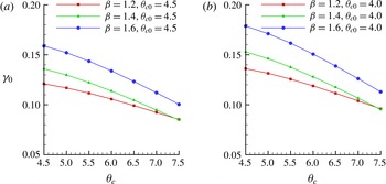
by considering fixed values for $\unicode[STIX]{x1D6FD}$ and $\unicode[STIX]{x1D703}_{c0}$ and fitting the value of $\unicode[STIX]{x1D6FE}_{0}$ . Considering two typical values of $\unicode[STIX]{x1D703}_{c0}=4.5$ and $4.0$ , we show in figure 2 the variation of the parameter $\unicode[STIX]{x1D6FE}_{0}$ with respect to $\unicode[STIX]{x1D703}_{c}$ for three values of the ellipticity parameter $\unicode[STIX]{x1D6FD}$ . Note the slow decrease in $\unicode[STIX]{x1D6FE}_{0}$ with $\unicode[STIX]{x1D703}_{c}$ (thus an increase in time). The values of $\unicode[STIX]{x1D6FE}_{0}$ shown in figure 2 are close to the one predicted by Kaplanski et al. (Reference Kaplanski, Fukumoto and Rudi2012): $\unicode[STIX]{x1D6FE}_{0}=0.16$ .

Figure 2.

The model parameter $\unicode[STIX]{x1D6FE}_{0}$ for two values of $\unicode[STIX]{x1D703}_{c0}$ and three values of the ellipticity parameter $\unicode[STIX]{x1D6FD}$ .

4 Predictions of the model versus direct numerical simulations

4.1 Physical and numerical parameters

The numerical code for solving the incompressible Navier–Stokes equations in cylindrical coordinates is described by Danaila et al. (Reference Danaila, Kaplanski and Sazhin2015) (see also Danaila & Helie Reference Danaila and Helie2008; Danaila, Vadean & Danaila Reference Danaila, Vadean and Danaila2009). The physical and numerical parameters used in our simulations are summarised below. The vortex ring was generated numerically by prescribing an appropriate axial velocity profile at the inlet section of the computational domain. This simulates the velocity profile produced by a vortex ring generator of piston/cylinder type. The main physical parameter of the flow is the Reynolds number based on the diameter $D$ of the vortex generator and the mean injection velocity $U_{0}$ :

(4.1)

$$\begin{eqnarray}\displaystyle Re_{D}=\frac{U_{0}D}{\unicode[STIX]{x1D708}}. & & \displaystyle\end{eqnarray}$$

Using the time scale $t_{0}=D/U_{0}$ , the non-dimensional time used in the simulations is defined as $\unicode[STIX]{x1D70F}=tU_{0}/D$ . We consider only short injection times, as in experiments performed by Stewart et al. (Reference Stewart, Niebel, Jung and Vlachos2012). This allows us to prescribe the inflow velocity using the model suggested by Danaila et al. (Reference Danaila, Vadean and Danaila2009):

(4.2)

$$\begin{eqnarray}\displaystyle U_{in}(r,\unicode[STIX]{x1D70F})=U_{0}U_{p}(\unicode[STIX]{x1D70F})U_{CL}(\unicode[STIX]{x1D70F})U_{b}(r,\unicode[STIX]{x1D70F}),\quad 0<\unicode[STIX]{x1D70F}\leqslant \unicode[STIX]{x1D70F}_{off}, & & \displaystyle\end{eqnarray}$$

where $U_{p}(\unicode[STIX]{x1D70F})$ is the piston velocity program (normalised by its maximum value $U_{0}$ ), $U_{CL}(\unicode[STIX]{x1D70F})$ takes into account the time evolution of the centreline velocity,

(4.3)

$$\begin{eqnarray}\displaystyle U_{CL}(\unicode[STIX]{x1D70F})=\frac{1}{\displaystyle 1-\frac{8}{\sqrt{\unicode[STIX]{x03C0}Re_{D}}}\sqrt{\unicode[STIX]{x1D70F}}+\displaystyle \frac{8}{Re_{D}}\unicode[STIX]{x1D70F}} & & \displaystyle\end{eqnarray}$$

and $U_{b}(r,\unicode[STIX]{x1D70F})$ describes the radial dependence of the profile

(4.4)

$$\begin{eqnarray}\displaystyle \hspace{-15.00002pt}U_{b}(r,\unicode[STIX]{x1D70F})=\frac{1}{2}\left\{1+\tanh \left[\frac{1}{4\unicode[STIX]{x1D6E9}(\unicode[STIX]{x1D70F})}\left(1-\frac{r}{R_{jet}(\unicode[STIX]{x1D70F})}\right)\right]\right\}, & & \displaystyle\end{eqnarray}$$

(4.5a-c )

$$\begin{eqnarray}\displaystyle \hspace{-15.00002pt}\unicode[STIX]{x1D6E9}(\unicode[STIX]{x1D70F})=\frac{\sqrt{2}-1}{\sqrt{\unicode[STIX]{x03C0}}}B(\unicode[STIX]{x1D70F}),\quad R_{jet}(\unicode[STIX]{x1D70F})=\frac{1}{2}-0.477B(\unicode[STIX]{x1D70F}),\quad B(\unicode[STIX]{x1D70F})=\frac{2}{\sqrt{Re_{D}}}\sqrt{\unicode[STIX]{x1D70F}}. & & \displaystyle\end{eqnarray}$$

For the piston velocity program we used the model suggested by Zhao, Steven & Mongeau (Reference Zhao, Steven and Mongeau2000):

(4.6)

$$\begin{eqnarray}\displaystyle U_{p}(\unicode[STIX]{x1D70F})=\left\{\begin{array}{@{}ll@{}}\displaystyle \frac{1}{2}\left[1-\cos \left(\unicode[STIX]{x03C0}\frac{\unicode[STIX]{x1D70F}}{\unicode[STIX]{x1D70F}_{1}}\right)\right], & \unicode[STIX]{x1D70F}\leqslant \unicode[STIX]{x1D70F}_{1}\\ \displaystyle \frac{1}{2}\left[1+\cos \left(\unicode[STIX]{x03C0}\frac{\unicode[STIX]{x1D70F}-\unicode[STIX]{x1D70F}_{1}}{\unicode[STIX]{x1D70F}_{2}-\unicode[STIX]{x1D70F}_{1}}\right)\right], & \unicode[STIX]{x1D70F}_{1}<\unicode[STIX]{x1D70F}\leqslant \unicode[STIX]{x1D70F}_{2}\approx \unicode[STIX]{x1D70F}_{off}.\end{array}\right. & & \displaystyle\end{eqnarray}$$

Function (4.6) gives a good approximation of the piston velocity $U_{p}(\unicode[STIX]{x1D70F})$ observed by Stewart et al. (Reference Stewart, Niebel, Jung and Vlachos2012).

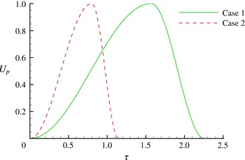
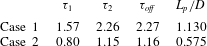
We consider the following two cases described in table 1. Case 1 (see figure 3, the solid curve) corresponds to experiments by Stewart et al. (Reference Stewart, Niebel, Jung and Vlachos2012) and was considered by Danaila et al. (Reference Danaila, Kaplanski and Sazhin2015) to test the VRC model. It will be used to compare the two confined vortex ring models. A shorter injection program was considered for Case 2 (see figure 3, the dashed curve), giving an approximatively two times smaller piston stroke ratio $L_{p}/D$ . Case 2 is expected to produce vortex rings with less elongated cores. Note that these stroke ratios are lower than the so-called formation number of the vortex ring, reported to be in the range 3.6 to 4.5 (see Gharib, Rambod & Shariff Reference Gharib, Rambod and Shariff1998; Krueger & Gharib Reference Krueger and Gharib2003; Dabiri & Gharib Reference Dabiri and Gharib2005). This implies that all the vorticity produced by the vortex generator is expected to be engulfed by the vortex ring.

Figure 3.

Piston velocity $U_{p}(\unicode[STIX]{x1D70F})$ used for the direct numerical simulation cases described in table 1. Case 1 refers to the recent experiments by Stewart et al. (Reference Stewart, Niebel, Jung and Vlachos2012).

Table 1.

Parameters $\unicode[STIX]{x1D70F}_{1},\unicode[STIX]{x1D70F}_{2},\unicode[STIX]{x1D70F}_{off}$ of the injection program (4.6) and piston stroke ratios $L_{p}/D=\int _{0}^{\unicode[STIX]{x1D70F}_{off}}U_{p}(\unicode[STIX]{x1D70F})\,\text{d}\unicode[STIX]{x1D70F}$ used for Cases 1 and 2 of direct numerical simulations.

In all simulations the Reynolds number was set to $Re_{D}=3400$ , as in Danaila et al. (Reference Danaila, Kaplanski and Sazhin2015), since this relatively high value proved challenging in testing the VRC model. The length of the computational domain was taken as $L_{d}=8$ , which allowed us to avoid the vortex ring coming close to the downstream boundary. The grid was uniform in both axial and radial directions with a refined grid size $\unicode[STIX]{x1D6FF}r=\unicode[STIX]{x1D6FF}x=0.01$ which ensures grid convergence of the results. Tests with a stretched grid in the radial direction, such that at least 30 grid points are clustered in the vorticity layer at the inflow, showed identical results. The time step was set to $\unicode[STIX]{x1D6FF}\unicode[STIX]{x1D70F}=0.001$ , which is below the admissible value imposed by the stability requirement of the numerical scheme. Time step refinement tests showed negligible differences in the results obtained for lower $\unicode[STIX]{x1D6FF}\unicode[STIX]{x1D70F}$ .

4.2 Post-processing and comparison procedure

The numerically generated vortex ring forms rapidly due to very small piston stroke ratios. During the injection phase, a negative vorticity layer is generated at the lateral wall, with intensity depending on the confinement. After the injection stops ( $\unicode[STIX]{x1D70F}>\unicode[STIX]{x1D70F}_{off}$ ), a stopping vortex forms at the inlet section. To properly separate the vortex ring both from the vorticity layer at the wall and from the stopping vortex, we designed a special post-processing program, based on the free finite-element solver FreeFem++ (see Hecht Reference Hecht2012, Reference Hecht2016). The velocity field obtained from the direct numerical simulations (DNS) using second-order finite-difference schemes is easily represented as a finite-element field by splitting the rectangular finite-difference cell into two triangles. The DNS values at the computational nodes are then used to completely represent the velocity field as a $P_{1}$ (piecewise linear) function on the triangular mesh. This procedure avoids interpolations between the DNS field and its representation on the finite-element grid. It is also consistent with the second order spatial accuracy of the Navier–Stokes solver. The post-processing program then identifies all closed contours for the prescribed threshold of $\unicode[STIX]{x1D714}/\unicode[STIX]{x1D714}_{max}$ , selects the unique contour around the vortex ring centre to define the vortex ring domain ${\mathcal{D}}_{VR}$ and then meshes this new domain with triangles. The interpolation between different finite-element meshes is also $P_{1}$ , preserving the order of the accuracy of the finite-element representation. Since the initial finite-difference mesh is very refined, the resulting interpolation errors have no impact upon the integral values computed in the post-processing part.The advantage of this finite-element post-processing is that it enables us to represent accurately and smoothly the boundary of the vortex core and then to use high-order (up to seventh-order) Gauss methods to compute the integral characteristics (circulation, impulse, energy). For example, flow circulation and energy are computed as

(4.7a,b )

$$\begin{eqnarray}\displaystyle \unicode[STIX]{x1D6E4}=\iint _{{\mathcal{D}}_{VR}}\unicode[STIX]{x1D714}\,\text{d}r\,\text{d}x,\quad E=\unicode[STIX]{x03C0}\iint _{{\mathcal{D}}_{VR}}\unicode[STIX]{x1D714}\unicode[STIX]{x1D6F9}\,\text{d}r\,\text{d}x. & & \displaystyle\end{eqnarray}$$

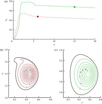
The time evolution of the circulation $\unicode[STIX]{x1D6E4}$ defined by (4.7) is shown in figure 4(a) for a confinement parameter $D_{w}/D=3$ , with $D_{w}$ being the diameter of the tube. Figure 4(b,c) illustrate the vortex ring domain ${\mathcal{D}}_{VR}$ computed with the post-processing program as the contour for which $\unicode[STIX]{x1D714}/\unicode[STIX]{x1D714}_{max}=0.05$ .

Figure 4.

Results of the direct numerical simulation of a confined vortex ring for $D_{w}/D=3$ and $Re_{D}=3400$ . (a) Time evolution of the vortex ring circulation for the cases described in table 1: Case 1 ( $L_{p}/D=1.13$ , solid curve) and Case 2 ( $L_{p}/D=0.575$ , dashed curve). Contours of vorticity $\unicode[STIX]{x1D714}/(U_{0}/D)$ corresponding to: (b) Case 2, $\unicode[STIX]{x1D70F}=6$ and (c) Case 1, $\unicode[STIX]{x1D70F}=15$ . In (b,c) the boundaries of the vortex ring domain ${\mathcal{D}}_{VR}$ , defined as the contour of $\unicode[STIX]{x1D714}=0.05\unicode[STIX]{x1D714}_{max}$ , are plotted as thick black contours.

After the separation of the vortex ring domain ${\mathcal{D}}_{VR}$ at a given time instant $\unicode[STIX]{x1D70F}=\unicode[STIX]{x1D70F}_{f}$ , we can use a nonlinear fit of the DNS vorticity with the VRE model (see (2.13)). Remembering that $I_{1}(z)\approx \exp (z)/\sqrt{2\unicode[STIX]{x03C0}z}$ for large $z$ , the vorticity distribution (2.13) can be approximated as:

(4.8)

$$\begin{eqnarray}\displaystyle \unicode[STIX]{x1D714}_{ef}=\frac{\unicode[STIX]{x1D6E4}_{ef}}{\unicode[STIX]{x03C0}}\left(\frac{R_{0f}}{r}\right)^{1/2}\frac{1}{2\unicode[STIX]{x1D6FD}L_{ef}^{2}}\exp \left(-\frac{1}{2L_{ef}^{2}}(r-R_{0f})^{2}-\frac{1}{2(\unicode[STIX]{x1D6FD}L_{ef})^{2}}(x-X_{0f})^{2}\right). & & \displaystyle\end{eqnarray}$$

Since FreeFem++ is interfaced to the state-of-the-art optimiser Ipopt, using the interior point minimisation method suggested by Wächter (Reference Wächter2002) and Wächter & Biegler (Reference Wächter and Biegler2006), we use a nonlinear fit procedure inside the finite-element post-processing to compute the five independent parameters in (4.8): $\unicode[STIX]{x1D6E4}_{ef},R_{0f},X_{0f},1/2L_{ef}^{2},1/2\unicode[STIX]{x1D6FD}^{2}L_{ef}^{2}$ . We finally compute $\unicode[STIX]{x1D703}_{ef}=R_{0f}/L_{ef}$ to complete the definition of the corresponding theoretical vortex ring. Formula (2.13) is then used to reconstruct the theoretical vorticity field $\unicode[STIX]{x1D714}(r,x)$ and compute integral characteristics in the same way as in DNS (taking into account only the vorticity of the vortex core for which $\unicode[STIX]{x1D714}/\unicode[STIX]{x1D714}_{max}>0.05$ ).

4.3 Assessment of the new model

Figure 4 shows the time evolution of the circulation $\unicode[STIX]{x1D6E4}$ for the two cases shown in table 1. We focus on the case of the confined vortex ring with $Re_{D}=3400$ and $D_{w}/D=3$ , for which we expect an improvement in theoretical predictions with respect to the VRC model presented in Danaila et al. (Reference Danaila, Kaplanski and Sazhin2015). After rapid increase during the injection phase, the circulation attains a small plateau and then starts to decrease during the post-formation phase. The decrease rate of the circulation induced by the presence of the lateral wall was investigated experimentally by Stewart et al. (Reference Stewart, Niebel, Jung and Vlachos2012) and numerically by Danaila et al. (Reference Danaila, Kaplanski and Sazhin2015). For the comparison between the vortex ring models, we selected time instants in the post-formation phase of the vortex ring: $\unicode[STIX]{x1D70F}=15$ for Case 1 (the same was used by Danaila et al. 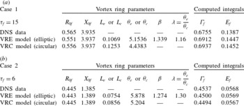(Reference Danaila, Kaplanski and Sazhin2015) to test the VRC model) and $\unicode[STIX]{x1D70F}=6$ for Case 2. The corresponding vortex ring vorticity contours are shown in figure 4. The results of the fit with both models VRE (elliptic core) and VRC (circular core) are summarised in table 2.

Table 2.

Parameters describing the geometry of the vortex ring used in models VRE (elliptic) and VRC (circular) for cases described in table 1. Vortex ring parameters ( $R_{0f},X_{0f},L,\unicode[STIX]{x1D703}$ ) are computed by a nonlinear fit of (4.8) using DNS data. Integral quantities (circulation $\unicode[STIX]{x1D6E4}_{f}$ and energy $E_{f}$ ) are then computed from models by reconstructing the vorticity field ((2.10) and (2.13)) and applying the same post-processing procedure as for the DNS fields (see § 4.2). $Re_{D}=3400$ , $D_{w}/D=3$ .

Figure 5.

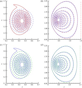
Contours of normalised vorticity $\unicode[STIX]{x1D714}/\unicode[STIX]{x1D714}_{max}$ (a,c) and corresponding normalised streamfunction $\unicode[STIX]{x1D713}/\unicode[STIX]{x1D713}_{max}$ (b,d), predicted by DNS (solid curves), the VRC (circular) model (a,b) and VRE (elliptic) model (c,d) (dashed curves). The values of $\unicode[STIX]{x1D714}/\unicode[STIX]{x1D714}_{max}$ and $\unicode[STIX]{x1D713}/\unicode[STIX]{x1D713}_{max}$ are shown from 0.1 to 0.9 with increments of 0.1. Case 2, $L_{p}/D=0.575$ , $Re_{D}=3400$ , $D_{w}/D=3$ , $\unicode[STIX]{x1D70F}=6$ .

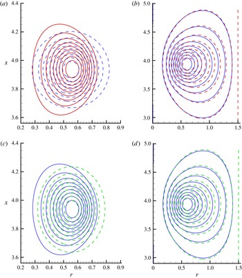
As expected, Case 2 produces a vortex ring which is not very elongated (see figure 4 b), but has large vorticity. As can be seen from table 2(b), the values of the circulation $\unicode[STIX]{x1D6E4}_{f}$ and energy $E_{f}$ computed from (4.7) are very close to DNS values, for both VRE and VRC models. A more detailed comparison of the models is offered by the plots of the vorticity and streamfunction distributions. Figure 5(a,c) show that the VRE model allows more accurate description of the vorticity distribution of the vortex core than the VRC model. At the same time, the prediction of the streamfunction distribution is only slightly improved in the VRE model, confirming the hypothesis that the streamfunction is not sensitive to the details of the vorticity distribution (see figure 5 b,d).

Figure 6.

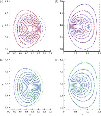
Contours of normalised vorticity $\unicode[STIX]{x1D714}/\unicode[STIX]{x1D714}_{max}$ (a,c) and corresponding normalised streamfunction $\unicode[STIX]{x1D713}/\unicode[STIX]{x1D713}_{max}$ (b,d), predicted by DNS (solid curves), the VRC (circular) model (a,b) and VRE (elliptic) model (c,d) (dashed curves). The values of $\unicode[STIX]{x1D714}/\unicode[STIX]{x1D714}_{max}$ and $\unicode[STIX]{x1D713}/\unicode[STIX]{x1D713}_{max}$ are shown from 0.1 to 0.9 with increments of 0.1. Case 1, $L_{p}/D=1.13$ , $Re_{D}=3400$ , $D_{w}/D=3$ , $\unicode[STIX]{x1D70F}=15$ .

The vortex ring in Case 1 (see figure 4 c) is more elongated ( $\unicode[STIX]{x1D6FD}\approx 1.34$ ) than in Case 2. Figure 6 shows that the fit with the VRE model offers a more accurate description of both vorticity and streamfunction distributions when compared to the VRC model. The integral quantities in table 2 display similar values for $\unicode[STIX]{x1D70F}=15$ . Note that the position of the vortex centre ( $R_{0f},X_{0f}$ ) and the circulation $\unicode[STIX]{x1D6E4}_{ef}$ needed in the model (see (2.13)) are not taken from DNS but computed using the global fitting procedure. This explains why, in figures 5 and 6, the centres of the fitted vortices are slightly shifted when compared to the DNS values. The elliptic shape assumed in our model approximates reasonably accurately the geometry of the DNS vortex ring, but this approximation is not perfect. The actual shape of vortex rings deviates from the theoretical elliptic one.

A different fitting procedure was also tested: the values for ( $R_{0f},X_{0f},\unicode[STIX]{x1D6E4}_{ef}$ ) were taken from DNS and the remaining parameters were fitted by a nonlinear procedure, one parameter ( $L_{c}$ ) for the circular VRC model and two parameters ( $L_{ef}$ and $\unicode[STIX]{x1D6FD}$ ) for the elliptic VRE model. This new fitting procedure has the advantage of being very fast and more convenient for a practical application of the model to describe actual experimental or numerically generated vortex rings. It can also be useful for the reconstruction of the velocity field generated around a vortex ring when only incomplete measurements of the velocity are available (see Zhang & Danaila Reference Zhang and Danaila2012; Danaila & Protas Reference Danaila and Protas2015). Figure 7 illustrates the obtained results for Case 1: the centre of the vortex is more accurately described with this partial fitting procedure, but only for the elliptic vortex model. The obtained values for the geometric parameters are very similar (compared to values displayed in table 2): $\unicode[STIX]{x1D703}_{c}=4.556$ (for the VRC model) and $\unicode[STIX]{x1D703}_{e}=5.19,\unicode[STIX]{x1D6FD}=1.28$ (for the VRE model).

Figure 7.

Same legend as in figure 6. Results obtained using a partial fitting procedure for the parameters of the models: ( $R_{0f},X_{0f},\unicode[STIX]{x1D6E4}_{ef}$ ) are taken from DNS and only one parameter ( $L_{c}$ ) for the circular VRC model and two parameters ( $L_{ef}$ and $\unicode[STIX]{x1D6FD}$ ) for the elliptic VRE model fitted by a nonlinear procedure.

Figure 8.

Time evolution of energy $E$ (a) and translational velocity $U$ (b) of the vortex ring as computed by DNS (solid curve) and predicted by models: VRC (circular) model (dashed curve) and VRE (elliptic) model (dashed-dotted curve). Case 1, $L_{p}/D=1.13$ , $Re_{D}=3400$ , $D_{w}/D=3$ . Vortex ring geometric parameters are fitted from DNS only at time instant $\unicode[STIX]{x1D70F}=15$ : (a,b) full fitting procedure (fit of four parameters for the VRC model and five parameters for the VRE model); (c,d) partial fitting procedure (fit of one parameter for the VRC model and two parameters for the VRE model).

To push the comparison procedure further and to compare the two fitting procedures, we predicted the time evolution of the energy $E$ and translational velocity $U$ , using the power law (2.7) for both $\unicode[STIX]{x1D703}_{c}$ and $\unicode[STIX]{x1D703}_{e}$ . More specifically, after fitting the DNS vortex with the prediction of the model at $\unicode[STIX]{x1D70F}=\unicode[STIX]{x1D70F}_{f}$ , we assumed that the model parameter depends on time as:

(4.9a,b )

$$\begin{eqnarray}\displaystyle \unicode[STIX]{x1D703}_{e}(\unicode[STIX]{x1D70F})=(\unicode[STIX]{x1D703}_{e})_{f}\left(\frac{\unicode[STIX]{x1D70F}_{f}}{\unicode[STIX]{x1D70F}}\right)^{1/2},\quad \unicode[STIX]{x1D6FD}=\text{const.},\quad \unicode[STIX]{x1D70F}\geqslant \unicode[STIX]{x1D70F}_{f}. & & \displaystyle\end{eqnarray}$$

Vorticity and streamfunction fields were then predicted for each time instant and the energy was computed from (4.7). The values of the translational velocity predicted by the model were computed from the equation (see Helmholtz Reference Helmholtz1867; Lamb Reference Lamb1932):

(4.10)

$$\begin{eqnarray}\displaystyle U_{VRE}=\frac{R_{0f}}{\unicode[STIX]{x1D6E4}_{f}}\int _{-\infty }^{\infty }\int _{0}^{R_{w}}\left(\unicode[STIX]{x1D6F9}_{VRE}^{w}-6x\frac{\unicode[STIX]{x2202}\unicode[STIX]{x1D6F9}_{VRE}^{w}}{\unicode[STIX]{x2202}x}\right)\unicode[STIX]{x1D714}_{VRE}\,\text{d}r\,\text{d}x\bigg/\!\left(2\int _{-\infty }^{\infty }\int _{0}^{R_{w}}r^{2}\unicode[STIX]{x1D714}_{VRE}\,\text{d}r\,\text{d}x\right). & & \displaystyle \nonumber\\ \displaystyle & & \displaystyle\end{eqnarray}$$

The non-dimensional translational velocity of the vortex ring was computed from DNS data as:

(4.11a,b )

$$\begin{eqnarray}\displaystyle U_{DNS}=\frac{\text{d}X_{\unicode[STIX]{x1D714}}}{\text{d}\unicode[STIX]{x1D70F}},\quad X_{\unicode[STIX]{x1D714}}=\int _{-\infty }^{\infty }\int _{0}^{R_{w}}r^{2}x\unicode[STIX]{x1D714}\,\text{d}x\,\text{d}r\bigg/\!\int _{-\infty }^{\infty }\int _{0}^{R_{w}}r^{2}\unicode[STIX]{x1D714}\,\text{d}x\,\text{d}r, & & \displaystyle\end{eqnarray}$$

where $X_{\unicode[STIX]{x1D714}}$ is the streamwise coordinate of the vorticity centroid (see Saffman Reference Saffman1970).

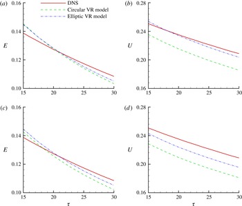
We display in figure 8 the model predictions for the time evolution of the energy $E$ and translational velocity $U$ for $D_{w}/D=3$ . For this case, the influence of the boundary layer generated at the lateral wall is weak during the post-formation phase, which is in agreement with the hypothesis of the model. As a consequence, the translational velocity predicted by the VRE model is closer to DNS results than the prediction of the VRC model. This result is consistent with the results of Kaplanski et al. (Reference Kaplanski, Fukumoto and Rudi2012) showing that the elliptic vortex ring model allows for better predictions of the translational velocity of the unbounded vortex ring, when compared to previously developed models (Fukumoto & Moffatt Reference Fukumoto and Moffatt2008).

Figure 8 also compares the accuracy of the model predictions when different fitting procedures are used. As one would expect, the full fitting procedure (figure 8 a,b) gives a better approximation of the time evolution of both energy and translational velocity. However, the partial fitting procedure (which is faster and very easy to implement) offers a fairly good approximation (figure 8 c,d), suggesting that the model is sufficiently robust for the description of actual vortex ring flows.

Figures 6 and 8 show that the new model offers a more accurate description of the geometry of the vortex core and a more accurate prediction of the translational velocity. This is expected to be particularly important for practical applications, including those in gasoline internal combustion engines where vortex ring type flow is used to form a kernel for the ignition of a combustible mixture (Heywood Reference Heywood1988).

4.4 Vortex ring geometry and the effect of the confinement

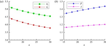
The new VRE model was applied to describe the vortex ring geometry during the post-formation phase. The results for Cases 1 and 2 turned out to be qualitatively similar; we show here only the results referring to Case 1. Figure 9(a) shows that parameters $\unicode[STIX]{x1D703}_{c}$ , $\unicode[STIX]{x1D703}_{e}$ , describing viscous effects (see (2.14)), slowly decrease during the post-formation phase, indicating that the vortex ring grows by viscous dissipation. The elongation of the vortex ring, quantified by parameter $\unicode[STIX]{x1D6FD}$ , increases over time, while the compression $\unicode[STIX]{x1D706}$ is quasi-constant during a long period of time (see figure 9 b).

Figure 9.

Time evolution of the parameters describing the vortex ring geometry during the post-formation phase. Parameters $\unicode[STIX]{x1D703}_{c}$ , $\unicode[STIX]{x1D703}_{e}$ are related to the viscous length of the model (2.14), while $\unicode[STIX]{x1D6FD}>0$ and $\unicode[STIX]{x1D706}>0$ describe the elongation and compression along axes $x$ and $r$ , respectively. All parameters are fitted from DNS data for Case 1, $L_{p}/D=1.13$ , $Re_{D}=3400$ , $D_{w}/D=3$ .

Figure 10.

Effect of confinement $D_{w}/D$ on time evolution of parameters $\unicode[STIX]{x1D6FD}>0$ and $\unicode[STIX]{x1D706}>0$ describing the extension and compression along axes $x$ and $r$ , respectively. All parameters are fitted from DNS data for Case 1, $L_{p}/D=1.13$ , $Re_{D}=3400$ .

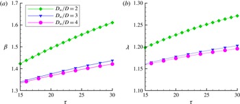
The influence of the confinement ratio $D_{w}/D$ on the time evolution of parameters $\unicode[STIX]{x1D6FD}$ and $\unicode[STIX]{x1D706}$ is shown in figure 10. Note that the evolution of these parameters reflects the interaction of the vortex ring with the lateral wall. For high confinements ( $D_{w}/D=2$ ) the vortex ring continuously elongates and $\unicode[STIX]{x1D6FD}$ increases quasi-linearly. The rate of increase of $\unicode[STIX]{x1D6FD}$ diminishes for lower confinements ( $D_{w}/D=3$ ). Note that in predicting the time evolution of the energy and translational velocity in figure 8 we assumed that $\unicode[STIX]{x1D6FD}$ was constant in time (see (4.9)), to facilitate the application of the model for actual vortex rings. Calculations with $\unicode[STIX]{x1D6FD}(\unicode[STIX]{x1D70F})$ represented by heuristic power laws (see also Kaplanski et al. Reference Kaplanski, Fukumoto and Rudi2012) can result in slightly improved values for the predicted integral characteristics. Lower variation rates are observed in figure 10(b) for the compression coefficient $\unicode[STIX]{x1D706}$ . The influence of the confinement on $\unicode[STIX]{x1D6FD}$ and $\unicode[STIX]{x1D706}$ can be considered negligible for $D_{w}/D\geqslant 3$ . This observation is in agreement with the hypothesis of the asymptotic analysis presented in § 3.1. It is also interesting to note from figure 10(a) that the estimate $\unicode[STIX]{x1D6FD}=1.4$ inferred from the asymptotic analysis is compatible with the values of $\unicode[STIX]{x1D6FD}$ fitted from DNS data for $D_{w}/D\geqslant 3$ .

5 An heuristic relation between vortex ring energy and circulation

In this section, we will show that the model developed above can be applied in an area not directly related to vortex ring confinements.

Recently, Krieg & Mohseni (Reference Krieg and Mohseni2013) demonstrated that jet flows created from cylinder–piston mechanisms enter the reservoir with nearly parallel streamlines, whereas jets ejected through a circular orifice in a flat plate have a radial component of velocity, directed towards the axis. These authors pointed out that the converging radial velocity significantly increases the translational velocity of the produced vortex ring and proposed the well tested heuristic relation between its dimensionless energy $E_{d}=E/(M^{1/2}\unicode[STIX]{x1D6E4}^{3/2})$ and circulation $\unicode[STIX]{x1D6E4}_{d}=\unicode[STIX]{x1D6E4}/(M^{1/3}U^{2/3})$ , where $M$ is the impulse:

(5.1)

$$\begin{eqnarray}\displaystyle {\unicode[STIX]{x1D6E4}_{d}}^{3/2}=c_{1}+c_{2}/E_{d}, & & \displaystyle\end{eqnarray}$$

for a wide range of experimental results, where $c_{1}=1.13$ and $c_{2}=0.52$ . This relation provides a reliable tool to describe vortex rings at the initial stage of their development, when the identification of the pinch-off moment is difficult both numerically and experimentally. It allows us to approximate the translational velocity of the vortex ring ( $U$ ) as a function of the total circulation ( $\unicode[STIX]{x1D6E4}$ ), impulse ( $M$ ) and kinetic energy ( $E$ ) of the vortex system by the following relation:

(5.2)

$$\begin{eqnarray}\displaystyle U=\frac{\unicode[STIX]{x1D6E4}^{3/2}E}{c_{1}EM^{1/2}+c_{2}M\unicode[STIX]{x1D6E4}^{3/2}}. & & \displaystyle\end{eqnarray}$$

Krieg & Mohseni (Reference Krieg and Mohseni2013) showed that the Norbury family of vortex rings (Norbury Reference Norbury1973) satisfy (5.1) for a wide range of dimensionless core radii $\unicode[STIX]{x1D6FC}$ .

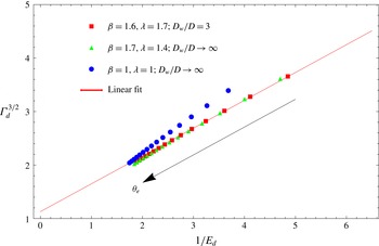
Figure 11 shows the plot of $\unicode[STIX]{x1D6E4}_{d}^{3/2}$ versus $1/E_{d}$ , for different vortex rings modelled with the present approach (confined elliptic, unconfined circular and unconfined elliptic). The values of $\unicode[STIX]{x1D6E4}_{d}$ and $E_{d}$ correspond to the range of $L=R_{0}/\unicode[STIX]{x1D703}_{e}=0.0952381-0.285714$ and $\unicode[STIX]{x1D703}_{e}=3.5-10.5$ ( $R_{0}=1$ ). Our aim is to find a set of geometric parameters for the vortex ring in order to obtain a linear variation of $\unicode[STIX]{x1D6E4}_{d}^{3/2}$ versus $1/E_{d}$ , as predicted by (5.1). As can be seen in this figure, the model with a circular core cannot be used to describe such vortex rings, while the elliptic vortex model could potentially model such flows. For both confined and unconfined elliptic vortices, the values of the geometrical parameters fitted to obtain curves describing the linear variation are indicated in the figure. We consider this to be an important generalisation of the above-mentioned result presented by Krieg & Mohseni (Reference Krieg and Mohseni2013) as our model is expected to describe the geometry of vortex rings more accurately than does the Norbury family of vortex rings. This further supports the importance of the new model described in our paper.

Figure 11.

The plot of $\unicode[STIX]{x1D6E4}_{d}^{3/2}$ versus $1/E_{d}$ , predicted by (5.1) (linear fit), and a set of values of $\unicode[STIX]{x1D6E4}_{d}^{3/2}$ and $1/E_{d}$ predicted by our model for various $\unicode[STIX]{x1D6FD}$ , $\unicode[STIX]{x1D706}$ and $D_{w}/D$ .

6 Summary and discussion

We suggested a new model that takes into account the elongated (elliptical) shape of confined vortex rings. The vorticity $\unicode[STIX]{x1D714}_{VRE}$ and streamfunction $\unicode[STIX]{x1D6F9}_{VRE}$ distributions based on the unconfined vortex ring model suggested in Kaplanski et al. (Reference Kaplanski, Fukumoto and Rudi2012) were used in the analysis. Using Brasseur’s method, a wall-induced streamfunction correction $\unicode[STIX]{x1D6F9}_{VRE}^{0}$ was analytically derived. The total streamfunction of the flow $\unicode[STIX]{x1D6F9}_{VRE}^{w}$ was presented as $\unicode[STIX]{x1D6F9}_{VRE}^{w}=\unicode[STIX]{x1D6F9}_{VRE}-\unicode[STIX]{x1D6F9}_{VRE}^{0}$ .

The new model was shown to describe accurately the geometry of the confined vortex ring and the time evolution of the vortex ring energy when compared with the results of direct numerical simulations. For large deformations of the vortex core, occurring for high confinements, the elliptical-core vortex ring model allows us to better predict the time evolution of the translational velocity than the circular vortex core model suggested by Danaila et al. (Reference Danaila, Kaplanski and Sazhin2015). This result was expected, remembering that the model derived by Kaplanski et al. (Reference Kaplanski, Fukumoto and Rudi2012) for an unconfined vortex ring with elliptical core offered a better estimation of the translational velocity at the whole post-formation stage when compared with experimental data presented by Weigand & Gharib (Reference Weigand and Gharib1997).

It is suggested that our model can be used to describe the deformation of the vortex ring during the post-formation phase. For long-time evolution, we derived a generalisation of the well-known Rott & Cantwell (Reference Rott and Cantwell1993) formula for the drift velocity of the vortex ring by taking into account the influence of the ellipticity parameter. When compared to experimental observations, it allows us to extract the value of the ellipticity parameter $\unicode[STIX]{x1D6FD}$ and thus to describe actual vortex rings with the present model. The fit of numerically or experimentally generated vortex rings with this model gives a synthetic view of the vortex elongation and compression along the longitudinal and radial axis. Two fitting procedures are suggested, computing all parameters (full fitting) or only geometrical parameters (partial fitting). The latter approach is very fast and easy to implement which makes it appropriate for practical applications involving the description of actual vortex rings or the reconstruction of their velocity field from incomplete measurements. Since the model is shown to be robust with respect to the fitting procedure, it is expected to be useful in practical applications where an accurate estimation of the vortex ring positions and geometry are required (e.g. applications in gasoline internal combustion engines, see Begg et al. (Reference Begg, Kaplanski, Sazhin, Hindle and Heikal2009)). It is shown that the predictions of the model support the recently suggested heuristic relation (Krieg & Mohseni Reference Krieg and Mohseni2013) between the energy and circulation of vortex rings in the case, where the injection velocity has a converging radial component. This is believed to be an interesting feature of the model and potentially useful for practical applications.

The analysis presented in this paper was focused on elongation parameters $\unicode[STIX]{x1D6FD}>1$ (i.e. $\unicode[STIX]{x1D716}_{0}>0$ in (2.15)) and confinement parameter $1<D_{w}/D\leqslant \infty$ , but the new model could be regarded as a unified theoretical framework for the following models: the VRE confined elliptic vortex ring ( $\unicode[STIX]{x1D6FD}>1$ ), the VRC confined circular vortex ring ( $\unicode[STIX]{x1D6FD}=1$ ) and the unconfined elliptic vortex ring (when $D_{w}/D\rightarrow \infty$ , correction (3.34) tends to zero). Figure 12 illustrates three possible vortex core geometries obtained for typical values of parameters $\unicode[STIX]{x1D6FD}$ and $D_{w}/D$ .

Figure 12.

An illustration of the models for confined and unconfined vortex rings with elliptical and circular cores. Isocontours of the streamfunction $\unicode[STIX]{x1D6F9}/\unicode[STIX]{x1D6F9}_{max}=0$ ; $0.1$ for $\unicode[STIX]{x1D6FD}=1.9,D_{w}=3$ (solid curve), $\unicode[STIX]{x1D6FD}=1,D_{w}/D=3$ (dashed curve) and $\unicode[STIX]{x1D6FD}=1$ , $D_{w}/D\rightarrow \infty$ (dot-dashed curve) with $R_{0}=1,\unicode[STIX]{x1D703}=3$ . The regions of vorticity $\unicode[STIX]{x1D714}/\unicode[STIX]{x1D714}_{max}\geqslant 0.05$ for vortex rings with elliptical (horizontal stripes) and circular (vertical stripes) cores.

Acknowledgements

The authors are grateful to EPSRC (grants EP/K005758/1 and EP/M002608/1) for financial support and to CRIHAN (Centre de Resources Informatiques de Haute-Normandie, France) for providing computational resources (project 2015001). I.D. acknowledges the generous hospitality of the Fields Institute, Toronto, during the Thematic Program on Multiscale Scientific Computing, January–April, 2016.

Appendix A. Proof of (3.30) for arbitrary $p$

In what follows the following identity will be proven:

(A 1)

$$\begin{eqnarray}\displaystyle \int _{0}^{\infty }\unicode[STIX]{x1D707}^{2p}\exp (-|\tilde{x}|\unicode[STIX]{x1D707})\text{J}_{0}(\tilde{\tilde{r}}\unicode[STIX]{x1D707})\,\text{d}\unicode[STIX]{x1D707}=\frac{2(-1)^{p}}{\unicode[STIX]{x03C0}}\int _{0}^{\infty }\unicode[STIX]{x1D707}^{2p}\text{K}_{0}(\tilde{\tilde{r}}\unicode[STIX]{x1D707})\cos (\unicode[STIX]{x1D707}\tilde{\tilde{x}})\,\text{d}\unicode[STIX]{x1D707}. & & \displaystyle\end{eqnarray}$$

The left and right parts of (A 1) can be calculated using Mathematica (2007) and presented in closed forms as:

(A 2)

$$\begin{eqnarray}\displaystyle & \displaystyle I_{1}=|\tilde{x}|^{-1-2p}\unicode[STIX]{x1D6E4}(1+2p)\text{}_{2}F_{1}\left(1/2+p,1+p;1;-\frac{\tilde{r}^{2}}{\tilde{x}^{2}}\right), & \displaystyle\end{eqnarray}$$

(A 3)

$$\begin{eqnarray}\displaystyle & \displaystyle I_{2}=\frac{(-1)^{p}2^{2p}}{\unicode[STIX]{x03C0}}\tilde{r}^{-1-2p}\unicode[STIX]{x1D6E4}(1/2+p)^{2}\text{}_{2}F_{1}\left(1/2+p,1/2+p;1/2;-\frac{\tilde{x}^{2}}{\tilde{r}^{2}}\right), & \displaystyle\end{eqnarray}$$

where

(A 4)

$$\begin{eqnarray}\displaystyle \text{}_{2}F_{1}(a,b;c;z)=\mathop{\sum }_{k=0}^{\infty }\frac{\left(a\right)_{k}(b)_{k}}{(c)_{k}}\frac{z^{k}}{k!} & & \displaystyle\end{eqnarray}$$

is the generalised hypergeometric function and $\unicode[STIX]{x1D6E4}(x)$ is the gamma function. The generalised hypergeometric function is presented as (Mathematica 2007):

(A 5)

$$\begin{eqnarray}\displaystyle \text{}_{2}F_{1}(a,b;c;z) & = & \displaystyle \frac{\unicode[STIX]{x1D6E4}(b-a)\unicode[STIX]{x1D6E4}(c)}{\unicode[STIX]{x1D6E4}(b)\unicode[STIX]{x1D6E4}(c-a)}_{2}F_{1}\left(a,a-c+1;a-b+1;\frac{1}{z}\right)\nonumber\\ \displaystyle & & \displaystyle +\,\frac{\unicode[STIX]{x1D6E4}(a-b)\unicode[STIX]{x1D6E4}(c)}{\unicode[STIX]{x1D6E4}(a)\unicode[STIX]{x1D6E4}(c-b)}_{2}F_{1}\left(b,b-c+1;-a+b+1;\frac{1}{z}\right).\end{eqnarray}$$

This allows us to present $I_{1}$ (see (A 2)) in the following form

(A 6)

$$\begin{eqnarray}\displaystyle I_{1} & = & \displaystyle |\tilde{x}|^{-1-2p}\unicode[STIX]{x1D6E4}(1+2p)\left[\left(\frac{\tilde{r}^{2}}{\tilde{x}^{2}}\right)^{-1-p}\frac{\unicode[STIX]{x1D6E4}(-1/2)\unicode[STIX]{x1D6E4}(1)}{\unicode[STIX]{x1D6E4}(-p)\unicode[STIX]{x1D6E4}(1/2+p)}_{2}F_{1}\left(1+p,1+p;3/2;-\frac{\tilde{x}^{2}}{\tilde{r}^{2}}\right)\right.\nonumber\\ \displaystyle & & \displaystyle \left.+\,\left(\frac{\tilde{r}^{2}}{\tilde{x}^{2}}\right)^{-1/2-p}\frac{\unicode[STIX]{x1D6E4}(1/2)\unicode[STIX]{x1D6E4}(1)}{\unicode[STIX]{x1D6E4}(1/2-p)\unicode[STIX]{x1D6E4}(1+p)}_{2}F_{1}\left(1/2+p,1/2+p;1/2;-\frac{\tilde{x}^{2}}{\tilde{r}^{2}}\right)\right].\end{eqnarray}$$

Taking into account that $\unicode[STIX]{x1D6E4}(-p)=\tilde{\infty };p\in N$ ( $\tilde{\infty }$ is complex infinity (Mathematica 2007)), we can ignore the first term in the square brackets. Remembering that $\unicode[STIX]{x1D6E4}(1)=1$ , and $\unicode[STIX]{x1D6E4}(1/2)=\sqrt{\unicode[STIX]{x03C0}}$ we obtain, after tedious but straightforward calculations

(A 7)

$$\begin{eqnarray}\displaystyle I_{1}=\frac{\sqrt{\unicode[STIX]{x03C0}}\unicode[STIX]{x1D6E4}(1+2p)}{\unicode[STIX]{x1D6E4}(1/2-p)\unicode[STIX]{x1D6E4}(1+p)}\tilde{r}^{-1-2p}\text{}_{2}F_{1}\left(1/2+p,1/2+p;1/2;-\frac{\tilde{x}^{2}}{\tilde{r}^{2}}\right). & & \displaystyle\end{eqnarray}$$

Remembering that $\unicode[STIX]{x1D6E4}(z)\unicode[STIX]{x1D6E4}(z+1/2)=\sqrt{\unicode[STIX]{x03C0}}2^{1-2z}\unicode[STIX]{x1D6E4}(2z)$ for $z=p+1/2$ (see Abramowitz & Stegun Reference Abramowitz and Stegun1964) we can write:

(A 8)

$$\begin{eqnarray}\displaystyle \frac{\unicode[STIX]{x1D6E4}(1+2p)}{\unicode[STIX]{x1D6E4}(1+p)}=\frac{2^{2p}\unicode[STIX]{x1D6E4}(1/2+p)}{\sqrt{\unicode[STIX]{x03C0}}}. & & \displaystyle\end{eqnarray}$$

Using the relations

(A 9a,b )

$$\begin{eqnarray}\displaystyle \frac{1}{\unicode[STIX]{x1D6E4}(1/2-p)}=\frac{(2p-1)!!}{(-2)^{p}\sqrt{\unicode[STIX]{x03C0}}},\quad \unicode[STIX]{x1D6E4}(1/2+p)=\sqrt{\unicode[STIX]{x03C0}}\frac{(2p-1)!!}{2^{p}}, & & \displaystyle\end{eqnarray}$$

we can estimate $I_{1}$ as

(A 10)

$$\begin{eqnarray}\displaystyle I_{1}=\frac{(-1)^{p}(2)^{2p}}{\unicode[STIX]{x03C0}}\unicode[STIX]{x1D6E4}(1/2+p)^{2}\tilde{r}^{-1-2p}\text{}_{2}F_{1}\left(1/2+p,1/2+p;1/2;-\frac{\tilde{x}^{2}}{\tilde{r}^{2}}\right). & & \displaystyle\end{eqnarray}$$

Thus, integral $I_{1}$ is identical to $I_{2}$ and (3.30) is proven.

References

Abramowitz, M. & Stegun, I. A. 1964 Handbook of Mathematical Functions. Dover.Google Scholar

Batchelor, G. K. 1988 An Introduction to Fluid Dynamics, 7th edn. Cambridge University Press.Google Scholar

Begg, S., Kaplanski, F., Sazhin, S., Hindle, M. & Heikal, M. 2009 Vortex ring-like structures in gasoline fuel sprays under cold-start conditions. Intl J. Engine Res. 10 (4), 195–214.CrossRef Google Scholar

Brasseur, J. G.1979 Kinematics and dynamics of vortex rings in a tube. NASA Tech. Rep. JIAA TR-26.Google Scholar

Brasseur, J. G.1986 Evolution characteristics of vortex rings over a wide range of Reynolds numbers. Proceedings of 4th AIAA/ASME Fluid Mechanics, Plasma Dynamics and Lasers Conference, May 12–14 1986, Atlanta, GA. AIAA Paper 86-1097.Google Scholar

Candon, S. & Marshall, J. 2012 Vortex ring deformation, capture, and entrainment by a columnar vortex. Phys. Fluids 24, 093604.CrossRef Google Scholar

Cater, J. E., Soria, J. & Lim, T. T. 2004 The interaction of the piston vortex with a piston-generated vortex ring. J. Fluid Mech. 499, 327–343.Google Scholar

Dabiri, J. O. & Gharib, M. 2005 Starting flow through nozzles with temporally variable exit diameter. J. Fluid Mech. 538, 111–136.Google Scholar

Danaila, I. & Helie, J. 2008 Numerical simulation of the postformation evolution of a laminar vortex ring. Phys. Fluids 20, 073602.CrossRef Google Scholar

Danaila, I., Kaplanski, F. & Sazhin, S. 2015 Modelling of confined vortex rings. J. Fluid Mech. 774, 267–297.Google Scholar

Danaila, I. & Protas, B. 2015 Optimal reconstruction of inviscid vortices. Proc. R. Soc. Lond. A 471, 20150323.Google Scholar

Danaila, I., Vadean, C. & Danaila, S. 2009 Specified discharge velocity models for the numerical simulation of laminar vortex rings. Theor. Comput. Fluid Dyn. 23, 317–332.Google Scholar

Fukumoto, Y. 2010 Global evolution of viscous vortex rings. Theor. Comput. Fluid Dyn. 24, 335–347.Google Scholar

Fukumoto, Y. & Moffatt, H. K. 2000 Motion and expansion of a viscous vortex ring. Part 1. A higher-order asymptotic formula for the velocity. J. Fluid Mech. 417, 1–45.Google Scholar

Fukumoto, Y. & Moffatt, H. K. 2008 Kinematic variational principle for motion of vortex rings. Physica D 237, 2210–2217.CrossRef Google Scholar

Gharib, M., Rambod, E., Kheradvar, A., Sahn, D. J. & Dabiri, J. O. 2006 Optimal vortex formation as an index of cardiac health. Proc. Natl Acad. Sci. 103, 6305–6308.Google Scholar

Gharib, M., Rambod, E. & Shariff, K. 1998 A universal time scale for vortex ring formation. J. Fluid Mech. 360, 121–140.CrossRef Google Scholar

Hecht, F. 2012 New developments in FreeFem++. J. Numer. Maths 20, 251–266.Google Scholar

Hecht, F.2016 FreeFem++ manual, version 3.49. www.freefem.org.Google Scholar

Helmholtz, H. 1867 On integrals of the hydrodynamical equations, which express vortex-motion. Phil. Mag. (4) 33, 485–510.Google Scholar

Heywood, J. B. 1988 Internal Combustion Engines Fundamentals. McGraw-Hill.Google Scholar

Kaplanski, F., Sazhin, S. S., Fukumoto, Y., Begg, S. & Heikal, M. 2009 A generalized vortex ring model. J. Fluid Mech. 622, 233–258.Google Scholar

Kaplanski, F. B., Fukumoto, Y. & Rudi, Y. A. 2012 Reynolds-number effect on vortex ring evolution in a viscous fluid. Phys. Fluids 24, 033101.Google Scholar

Kaplanski, F. B. & Rudi, Y. A. 1999 Dynamics of a viscous vortex ring. Intl J. Fluid Mech. Res. 26, 618–630.Google Scholar

Kaplanski, F. B. & Rudi, Y. A. 2005 A model for the formation of ‘optimal’ vortex ring taking into account viscosity. Phys. Fluids 17, 087101–087107.Google Scholar

Krieg, M. & Mohseni, K. 2013 On the approximation of the translational velocity of vortex rings. Trans. ASME J. Fluids Engng 135, 124501.Google Scholar

Krueger, S. & Gharib, M. 2003 The significance of vortex ring formation on the impulse and thrust of a starting jet. Phys. Fluids 15, 1271–1281.Google Scholar

Lamb, H. 1932 Hydrodynamics. Dover.Google Scholar

Lim, T. T. & Nickels, T. B. 1995 Vortex rings. In Vortices in Fluid Flows (ed. Green, S. I.), p. 95. Kluwer.Google Scholar

Mathematica2007 Version 6.0.0. Wolfram Research. http://functions.wolfram.com.Google Scholar

Norbury, J. 1973 A family of steady vortex rings. J. Fluid Mech. 57, 417–431.Google Scholar

Rott, N. & Cantwell, B. 1993 Vortex drift. I: dynamic interpretation. Phys. Fluids 5, 1443–1450.CrossRef Google Scholar

Saffman, P. G. 1970 The velocity of viscous vortex rings. Stud. Appl. Maths 49, 371.Google Scholar

Sazhin, S. S. 2014 Droplets and Sprays. Springer.Google Scholar

Shariff, K. & Leonard, A. 1992 Vortex rings. Annu. Rev. Fluid Mech. 24, 235–279.CrossRef Google Scholar

Stewart, K., Niebel, C., Jung, S. & Vlachos, P. 2012 The decay of confined vortex rings. Exp. Fluids 53, 163–171.Google Scholar

Wächter, A.2002 An interior point algorithm for large-scale nonlinear optimization with applications in process engineering. PhD thesis, Carnegie Mellon University, Pittsburgh, PA, USA.Google Scholar

Wächter, A. & Biegler, L. T. 2006 On the implementation of an interior-point filter line-search algorithm for large-scale nonlinear programming. Math. Program. 106, 25–57.CrossRef Google Scholar

Weigand, A. & Gharib, M. 1997 On the evolution of laminar vortex rings. Exp. Fluids 22, 447–457.Google Scholar

Zhang, Y. & Danaila, I. 2012 A finite element BFGS algorithm for the reconstruction of the flow field generated by vortex rings. J. Numer. Maths 20, 325–340.Google Scholar

Zhao, W., Steven, H. F. & Mongeau, L. G. 2000 Effects of trailing jet instability on vortex ring formation. Phys. Fluids 12, 589–596.Google Scholar

Figure 1.Schematic of a vortex ring in a tube. The elliptical core is described using two length scales: $L$ in the radial direction and $\unicode[STIX]{x1D6FD}L$ in the streamwise direction.

Figure 2.The model parameter $\unicode[STIX]{x1D6FE}_{0}$ for two values of $\unicode[STIX]{x1D703}_{c0}$ and three values of the ellipticity parameter $\unicode[STIX]{x1D6FD}$.

Figure 3.Piston velocity $U_{p}(\unicode[STIX]{x1D70F})$ used for the direct numerical simulation cases described in table 1. Case 1 refers to the recent experiments by Stewart et al. (2012).

Table 1.Parameters $\unicode[STIX]{x1D70F}_{1},\unicode[STIX]{x1D70F}_{2},\unicode[STIX]{x1D70F}_{off}$ of the injection program (4.6) and piston stroke ratios $L_{p}/D=\int _{0}^{\unicode[STIX]{x1D70F}_{off}}U_{p}(\unicode[STIX]{x1D70F})\,\text{d}\unicode[STIX]{x1D70F}$ used for Cases 1 and 2 of direct numerical simulations.

Figure 4.Results of the direct numerical simulation of a confined vortex ring for $D_{w}/D=3$ and $Re_{D}=3400$. (a) Time evolution of the vortex ring circulation for the cases described in table 1: Case 1 ($L_{p}/D=1.13$, solid curve) and Case 2 ($L_{p}/D=0.575$, dashed curve). Contours of vorticity $\unicode[STIX]{x1D714}/(U_{0}/D)$ corresponding to: (b) Case 2, $\unicode[STIX]{x1D70F}=6$ and (c) Case 1, $\unicode[STIX]{x1D70F}=15$. In (b,c) the boundaries of the vortex ring domain ${\mathcal{D}}_{VR}$, defined as the contour of $\unicode[STIX]{x1D714}=0.05\unicode[STIX]{x1D714}_{max}$, are plotted as thick black contours.

Table 2.Parameters describing the geometry of the vortex ring used in models VRE (elliptic) and VRC (circular) for cases described in table 1. Vortex ring parameters ($R_{0f},X_{0f},L,\unicode[STIX]{x1D703}$) are computed by a nonlinear fit of (4.8) using DNS data. Integral quantities (circulation $\unicode[STIX]{x1D6E4}_{f}$ and energy $E_{f}$) are then computed from models by reconstructing the vorticity field ((2.10) and (2.13)) and applying the same post-processing procedure as for the DNS fields (see § 4.2). $Re_{D}=3400$, $D_{w}/D=3$.

Figure 5.Contours of normalised vorticity $\unicode[STIX]{x1D714}/\unicode[STIX]{x1D714}_{max}$ (a,c) and corresponding normalised streamfunction $\unicode[STIX]{x1D713}/\unicode[STIX]{x1D713}_{max}$ (b,d), predicted by DNS (solid curves), the VRC (circular) model (a,b) and VRE (elliptic) model (c,d) (dashed curves). The values of $\unicode[STIX]{x1D714}/\unicode[STIX]{x1D714}_{max}$ and $\unicode[STIX]{x1D713}/\unicode[STIX]{x1D713}_{max}$ are shown from 0.1 to 0.9 with increments of 0.1. Case 2, $L_{p}/D=0.575$, $Re_{D}=3400$, $D_{w}/D=3$, $\unicode[STIX]{x1D70F}=6$.

Figure 6.Contours of normalised vorticity $\unicode[STIX]{x1D714}/\unicode[STIX]{x1D714}_{max}$ (a,c) and corresponding normalised streamfunction $\unicode[STIX]{x1D713}/\unicode[STIX]{x1D713}_{max}$ (b,d), predicted by DNS (solid curves), the VRC (circular) model (a,b) and VRE (elliptic) model (c,d) (dashed curves). The values of $\unicode[STIX]{x1D714}/\unicode[STIX]{x1D714}_{max}$ and $\unicode[STIX]{x1D713}/\unicode[STIX]{x1D713}_{max}$ are shown from 0.1 to 0.9 with increments of 0.1. Case 1, $L_{p}/D=1.13$, $Re_{D}=3400$, $D_{w}/D=3$, $\unicode[STIX]{x1D70F}=15$.

Figure 7.Same legend as in figure 6. Results obtained using a partial fitting procedure for the parameters of the models: ($R_{0f},X_{0f},\unicode[STIX]{x1D6E4}_{ef}$) are taken from DNS and only one parameter ($L_{c}$) for the circular VRC model and two parameters ($L_{ef}$ and $\unicode[STIX]{x1D6FD}$) for the elliptic VRE model fitted by a nonlinear procedure.

Figure 8.Time evolution of energy $E$ (a) and translational velocity $U$ (b) of the vortex ring as computed by DNS (solid curve) and predicted by models: VRC (circular) model (dashed curve) and VRE (elliptic) model (dashed-dotted curve). Case 1, $L_{p}/D=1.13$, $Re_{D}=3400$, $D_{w}/D=3$. Vortex ring geometric parameters are fitted from DNS only at time instant $\unicode[STIX]{x1D70F}=15$: (a,b) full fitting procedure (fit of four parameters for the VRC model and five parameters for the VRE model); (c,d) partial fitting procedure (fit of one parameter for the VRC model and two parameters for the VRE model).

Figure 9.Time evolution of the parameters describing the vortex ring geometry during the post-formation phase. Parameters $\unicode[STIX]{x1D703}_{c}$, $\unicode[STIX]{x1D703}_{e}$ are related to the viscous length of the model (2.14), while $\unicode[STIX]{x1D6FD}>0$ and $\unicode[STIX]{x1D706}>0$ describe the elongation and compression along axes $x$ and $r$, respectively. All parameters are fitted from DNS data for Case 1, $L_{p}/D=1.13$, $Re_{D}=3400$, $D_{w}/D=3$.

Figure 10.Effect of confinement $D_{w}/D$ on time evolution of parameters $\unicode[STIX]{x1D6FD}>0$ and $\unicode[STIX]{x1D706}>0$ describing the extension and compression along axes $x$ and $r$, respectively. All parameters are fitted from DNS data for Case 1, $L_{p}/D=1.13$, $Re_{D}=3400$.

Figure 11.The plot of $\unicode[STIX]{x1D6E4}_{d}^{3/2}$ versus $1/E_{d}$, predicted by (5.1) (linear fit), and a set of values of $\unicode[STIX]{x1D6E4}_{d}^{3/2}$ and $1/E_{d}$ predicted by our model for various $\unicode[STIX]{x1D6FD}$, $\unicode[STIX]{x1D706}$ and $D_{w}/D$.

Figure 12.An illustration of the models for confined and unconfined vortex rings with elliptical and circular cores. Isocontours of the streamfunction $\unicode[STIX]{x1D6F9}/\unicode[STIX]{x1D6F9}_{max}=0$; $0.1$ for $\unicode[STIX]{x1D6FD}=1.9,D_{w}=3$ (solid curve), $\unicode[STIX]{x1D6FD}=1,D_{w}/D=3$ (dashed curve) and $\unicode[STIX]{x1D6FD}=1$, $D_{w}/D\rightarrow \infty$ (dot-dashed curve) with $R_{0}=1,\unicode[STIX]{x1D703}=3$. The regions of vorticity $\unicode[STIX]{x1D714}/\unicode[STIX]{x1D714}_{max}\geqslant 0.05$ for vortex rings with elliptical (horizontal stripes) and circular (vertical stripes) cores.

Article contents

A model for confined vortex rings with elliptical-core vorticity distribution

Abstract

JFM classification

Information

1 Introduction

2 Background

3 Radially confined vortex rings with elliptical cores

3.1 Estimations of the ellipticity parameters

4 Predictions of the model versus direct numerical simulations

4.1 Physical and numerical parameters

4.2 Post-processing and comparison procedure

4.3 Assessment of the new model

4.4 Vortex ring geometry and the effect of the confinement

5 An heuristic relation between vortex ring energy and circulation

6 Summary and discussion

Acknowledgements

Appendix A. Proof of (3.30) for arbitrary $p$

References

Save article to Kindle

Save article to Dropbox

Save article to Google Drive

Reply to: Submit a response

Your details

You have entered the maximum number of contributors

Conflicting interests