1. Introduction
One of the interesting manifestations of turbulence is the occurrence of secondary flows in rectilinear flows. The most famous are the secondary flows in non-circular pipes. The change in the curvature of the wall along the perimeter of the cross-section of the pipe creates a spatial inhomogeneity of the Reynolds stresses and, as a consequence, motion in the plane perpendicular to the flow. Prandtl (Reference Prandtl1931) proposed to call such flows caused by Reynolds stresses secondary flows of the second kind, in contrast to secondary flows of the first kind, which arise in curved flows under the action of centrifugal effects in both turbulent and laminar flows. The characteristic velocities of secondary flows of the second kind are not high. They usually do not exceed a few percent of the mean bulk velocity. Nevertheless, their contribution to the transverse transport processes is comparable to the contribution of turbulent effects (Nikitin & Yakhot Reference Nikitin and Yakhot2005).
Many publications are devoted to the study and description of secondary flows of the second kind. Relevant references can be found in the recent in-depth reviews by Kornilov (Reference Kornilov2017) and Nikitin, Popelenskaya & Stroh (Reference Nikitin, Popelenskaya and Stroh2021). In most of the previous works, secondary flows were studied that arise in turbulent flows along internal longitudinal corners (for example, in rectangular ducts). Secondary flows along the external corners have been studied in less detail. Meanwhile, the study of fluid flow along the streamwise external corner is of significant importance not only in fundamental terms but also for various engineering applications. This flow includes many phenomena observed in turbulent flows encountered in practice, such as flows over turbine blades, flows in pipelines of complex internal cross-section, and flows along the edges and joints of surfaces on the hulls of land, air and water vehicles. Secondary flows arising in such configurations are much more intense compared to internal corner flows and are characterized by a number of other specific properties. We can only note the experiment carried out at the University of Melbourne by Panchapakesan & Joubert (Reference Panchapakesan and Joubert1998, Reference Panchapakesan and Joubert1999) and Moinuddin, Joubert & Chong (Reference Moinuddin, Joubert and Chong2004), and numerical simulations by Xu & Pollard (Reference Xu and Pollard2001) and Xu (Reference Xu2009). The experiment studied the flow along the edge formed by two flat plates joined at the right angle. It is found that the secondary flow in the cross-sectional plane has the form of a pair of vortices with opposite directions of rotation, located symmetrically relative to the corner bisector. The direction of fluid motion in the secondary flow is from the corner towards the outer flow along the bisector, and to the corner along the walls, i.e. the opposite to the secondary flows in internal corners. In the simulations, the flow in an annular square pipe was considered, in which there are four internal corners of  $90^\circ$ and four external corners of
 $270^\circ$. Although the Reynolds numbers in the simulation and experiment differed significantly, the results concerning the features of the secondary flow in the vicinity of external corners are in qualitative agreement. Works can also be noted in which turbulent flows over a flat surface in the presence of longitudinal inhomogeneities were studied. In Goldstein & Tuan (Reference Goldstein and Tuan1998), secondary flows over longitudinal ridges of triangular and rectangular shapes were investigated numerically. Secondary flows arising above the ridges are similar in shape to secondary flows along the external corners. It is hypothesized that the cause of the occurrence of secondary flows in this case is two-dimensional spanwise sloshing of the flow, inherent in a turbulent boundary layer, interacting with the stream-aligned element. Secondary flows over rectangular longitudinal irregularities were investigated in Vanderwel & Ganapathisubramani (Reference Vanderwel and Ganapathisubramani2015), Vanderwel et al. (Reference Vanderwel, Stroh, Kriegseis, Frohnapfel and Ganapathisubramani2019) and Hwang & Lee (Reference Hwang and Lee2018), both numerically and experimentally. The emergence of secondary flows with the rising fluid above the protruding elements of the surface was noted. The modification of the shape of secondary flows with a change in the size of protruding longitudinal inhomogeneities was studied in Castro et al. (Reference Castro, Kim, Stroh and Lim2021). The features of momentum and heat transfer over longitudinal triangular ribs were investigated in Stroh et al. (Reference Stroh, Schäfer, Forooghi and Frohnapfel2020). A noticeable increase in friction and heat transfer was found in comparison with a smooth surface.
It is generally assumed that secondary flows of the second kind are associated with turbulent flows and cannot develop in laminar flows. In fact, secondary flows can occur under the action of flow fluctuations, regardless of their nature. Fluctuations can be created by external artificial non-steady or spatially inhomogeneous influence, as well as by three-dimensional inhomogeneities of the boundary. Such an essentially laminar mechanism can lead to the emergence of secondary flows in both turbulent (Bhaganagar, Kim & Coleman Reference Bhaganagar, Kim and Coleman2004; Chan et al. Reference Chan, Macdonald, Chung, Hutchins and Ooi2018) and laminar (Elingsen, Akselsen & Chan Reference Elingsen, Akselsen and Chan2021) flows.
Considerable attention in studies of secondary flows of the second kind is paid to attempts to identify physical mechanisms and explain the causes of their occurrence. This is done traditionally by analysing the equation for the longitudinal component of the mean vorticity  $\varOmega _x = {\partial } W / {\partial } y- {\partial } V / {\partial } z$. Hereinafter,
 $(x, y, z)$ are Cartesian coordinates (the
 $x$ axis is directed along the flow), and
 $(u, v, w)$ and
 $(\omega _x, \omega _y, \omega _z)$ are the corresponding components of the velocity and vorticity vectors. Capital letters indicate mean values, and primes indicate fluctuations; statistical averaging is indicated by an overline. The equation for
 $\varOmega _x$ in a turbulent flow is
 \begin{equation} V\,\frac{{\partial}\varOmega_x}{{\partial} y}+W\,\frac{{\partial}\varOmega_x}{{\partial} z}-\nu\left(\frac{{\partial}^2 \varOmega_x}{{\partial} y^2}+\frac{{\partial}^2 \varOmega_x}{{\partial} z^2}\right)=S . \end{equation}
The flow is assumed to be steady in time and uniform in the longitudinal direction. Thus the mean values are independent of time and longitudinal coordinate. The source term on the right-hand side of (1.1) is responsible for the production of longitudinal vorticity. It is expressed through the Reynolds stress gradients
 \begin{equation} S=\frac{{\partial}^2}{{\partial} y\,{\partial} z}\left(\overline{v'^2}-\overline{w'^2}\right)+\left(\frac{{\partial}^2}{{\partial} z^2}-\frac{{\partial}^2}{{\partial} y^2}\right)\overline{v'w'} \equiv S_1+S_2 . \end{equation}
Many experimental, theoretical and computational works are devoted to the estimation of the source term  $S$ and the relative importance of its two components: the normal stress difference term
 $S_1$, and the shear stress term
 $S_2$ (see references and discussion in Nikitin Reference Nikitin2021; Nikitin et al. Reference Nikitin, Popelenskaya and Stroh2021). Representation of the source term in the form (1.2) was introduced in Einstein & Li (Reference Einstein and Li1958) for rectangular ducts, when the coordinate axes
 $y, z$ are parallel to the walls. This circumstance is sometimes overlooked, and the quantities
 $S_1, S_2$ are assigned a special physical meaning when analysing flows in pipes of arbitrary cross-section (Speziale Reference Speziale1982). Meanwhile,
 $S_1, S_2$ are not invariants; their values change when the coordinate system is rotated in the
 $(y, z)$ plane, and, in particular, change places when the axes are rotated by
 $45^\circ$ (Brundrett & Baines Reference Brundrett and Baines1964). Therefore, the use of the source term in the form (1.2) to describe secondary flows in pipes with a cross-section other than rectangular is not very productive. The values
 $S_1, S_2$, being non-zero individually, can completely neutralize each other, as happens, for example, in round pipes. Even in rectangular ducts
 $S_1, S_2$ have distributions similar in shape and opposite in sign, neutralizing each other by 90 % (Gavrilakis Reference Gavrilakis1992).
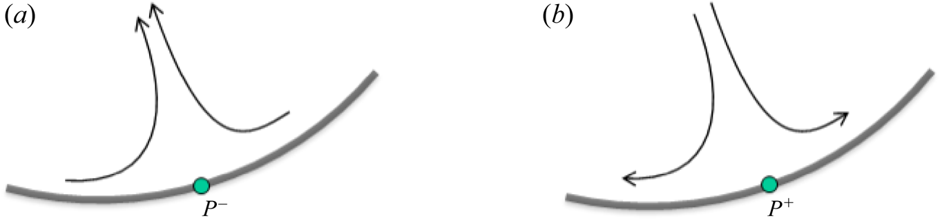
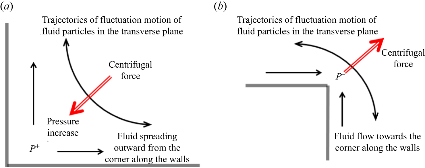
In Nikitin (Reference Nikitin2021) it is noted that the shape of the secondary flow near a solid wall is consistent with the distribution of the mean wall pressure. If the pressure changes along the wall, then a secondary flow must certainly arise, directed from higher pressure to a lower one. The secondary flow along the pipe wall is directed from the points of the local pressure maximum to the points of the local minimum. The consequence of this is the inflow of fluid to the wall from the outer flow to the points of local pressure maximum and, conversely, the outflow of the fluid from the wall to the outer flow at the points of the local pressure minimum. Streamlines in the vicinity of each local extremum of the mean wall pressure have the forms shown in figure 1. A change in the mean pressure along the perimeter can be caused by a change in the curvature of the wall, which is described below by the examples of flows in the vicinity of the internal and external corners of  $90^\circ$ (Nikitin et al. Reference Nikitin, Popelenskaya and Stroh2021). In the near-wall layer, tangential velocity fluctuations exceed normal fluctuations, so fluid particles move mainly parallel to the walls, and in the corner region, along arcuate trajectories joining directions along tangents to adjacent boundaries (figure 2). The resulting centrifugal force causes a change in the mean pressure in the corner. In the internal corner (figure 2a), an increase in pressure occurs, which leads to fluid spreading along the walls and a compensating inflow along the bisector. In the external corner, on the contrary, pressure decreases, leading to fluid flow along the walls into the corner region, and outward flow along the bisector (figure 2b). Thus the known patterns of secondary flows in the corner regions are formed.
The shapes of the secondary flow streamlines in the vicinity of the points of (a) local minimum  $P^-$, and (b) local maximum
 $P^+$, of the mean wall pressure (figure 5 of Nikitin Reference Nikitin2021).

The mechanism of secondary flow in the vicinity of (a) the internal corner, and (b) the external corner (figure 9 of Nikitin et al. Reference Nikitin, Popelenskaya and Stroh2021).

The examples considered in Nikitin (Reference Nikitin2021) confirm the presence of a local mean-pressure maximum at the internal corners, which is consistent with the qualitative explanation given above. However, the pressure distribution in the vicinity of the external corner turns out to be more complex. At the corner point, a local pressure minimum is actually reached if we consider its change at the surrounding points on the wall. This is sufficient for the appearance of a secondary flow pattern corresponding to figure 1(a). However, with distance from the corner point along the bisector, the pressure decreases, rather than increases, as the qualitative picture in figure 2(b) implies. Thus it turns out that the pressure force acts in the same direction as the centrifugal force, away from the corner. This indicates that this qualitative explanation of the cause of secondary flows near external corners at least requires clarification.
To study the details of turbulence and the mechanism of formation of secondary flows in the vicinity of the external longitudinal corner, in this work, direct numerical simulations of flows in a pipe with a cross-section in the form of a circular sector are performed. The chosen geometry allows calculations to be carried out in a simple orthogonal (cylindrical) coordinate system for any value of the apex angle  ${\alpha }$. The cases with
 ${\alpha } = 5{\rm \pi} /4$,
 $3{\rm \pi} /2$,
 $7{\rm \pi} /4$ and
 $2{\rm \pi}$ are considered. The study made it possible not only to obtain qualitative conclusions about the formation of secondary flows of Prandtl's second kind in turbulent flows along the external corners, but also to determine the quantitative characteristics of these flows at different values of the apex angle. As far as we know, this study is the first work in which results are obtained for different external corners. Despite the fact that the considered values of the Reynolds number are relatively small from the point of view of establishing the characteristics of turbulent flows, we hope that the obtained qualitative conclusions about the mechanisms and details of secondary flows along the external longitudinal corners will make sense for larger
 $Re$. Turbulent flows in pipes of the considered form have not been considered earlier in the literature. Therefore, we also provide a set of data on the statistical characteristics of these flows, although this is not the main purpose of the study. The paper also gives a short course on laminar flows in the geometry under consideration.
2. Laminar flow in a circular-sector pipe
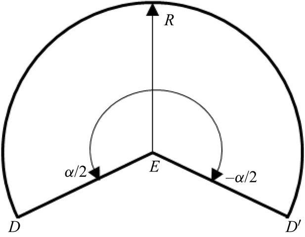
We consider the flow of a viscous incompressible fluid in a straight long pipe with a cross-section in the form of a circular sector of radius  $R$ and apex angle
 $\alpha$ (figure 3). The value of the angle
 $\alpha$ can range from
 $0$ to
 $2{\rm \pi}$. In this paper, main attention is paid to flows with
 $\alpha >{\rm \pi}$. In this case, the cross-section of the pipe has two internal concave corners (
 $D$ and
 $D'$ in figure 3) and one external convex corner (
 $E$).
Pipe cross-section with apex angle  $\alpha >{\rm \pi}$.

In the laminar flow regime, the velocity field has one non-zero component  $U(r,{\theta })$, the equation for which in the polar coordinate system
 $(r, {\theta })$ has the form
 \begin{equation} \frac{1}{r}\,\frac{{\partial}}{{\partial} r}r\,\frac{{\partial} U}{{\partial} r}+\frac{1}{r^2}\,\frac{{\partial}^2 U}{{\partial}\theta^2}=\frac{1}{\mu}\,\frac{{\rm d} P}{{\rm d}\kern0.7pt x} . \end{equation}
Here,  ${\rm d}P/{{\rm d}\kern0.7pt x}$ is a constant pressure gradient driving the flow, and
 $\mu$ is the viscosity of the fluid. The solution of (2.1) in the geometry under consideration is given in White (Reference White2006, equation (3-50)). The expression given in White (Reference White2006) has a singularity at
 $\cos {\alpha }= 0$ and leads to an indeterminate form of
 $\infty$–
 $\infty$ type, which makes it awkward to use. Here we give another form of solution.
We will measure the polar angle from the pipe symmetry plane; then the solution (2.1) with zero boundary condition can be represented as
 \begin{equation} U(r,\theta)=\sum_{n=1}^{\infty}U_n(r)\cos\beta_n\theta,\quad \beta_n=(2n-1){\rm \pi}/\alpha. \end{equation}
Substituting (2.2a,b) in (2.1) and applying the procedure of the Galerkin method, after simple manipulations, we get
 \begin{equation} U_n(r)={-}\frac{1}{\mu}\,\frac{{\rm d} P}{{\rm d}\kern0.7pt x}\,\frac{4r^2}{\rm \pi}\,\frac{({-}1)^{n-1}}{(2n-1)(\beta_n+2)}\times \left\{\!\!\begin{array}{ll} \dfrac{1-(r/R)^{\beta_n-2}}{\beta_n-2}, & \hbox{if}\ \beta_n\neq 2, \\ -\ln (r/R), & \hbox{if}\ \beta_n = 2. \end{array}\right. \end{equation}
The equality  $\beta _n = 2$ holds in two cases: for
 ${\alpha } = {\rm \pi}/2$,
 $n = 1$, and for
 ${\alpha } = 3{\rm \pi} /2$,
 $n = 2$. From (2.2a,b) and (2.3), the relationship between the bulk velocity
 $U_b$ and the pressure gradient can be found:
 \begin{equation} U_b={-}\frac{4R^2G}{{\rm \pi}^2}\,\frac{1}{\mu}\,\frac{{\rm d} P}{{\rm d}\kern0.7pt x}. \end{equation}
Here,
 \begin{equation} G(\alpha)=\sum_{n=1}^{\infty}\frac{1}{(2n-1)^2(\beta_n+2)^2} . \end{equation}
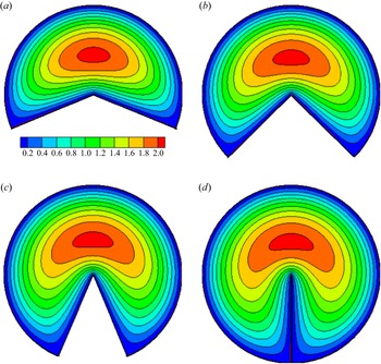
The distributions of the velocity  $U/U_b$ over the pipe cross-section for several values of
 ${\alpha }>{\rm \pi}$ are shown in figure 4. From (2.2a,b) and (2.3), it turns out that
 $U\sim r^{{\rm \pi} /{\alpha }}$ at
 $r\to 0$ for sufficiently large
 ${\alpha }>{\rm \pi} /2$. In particular, at
 ${\theta } = 0$,
 \begin{equation} \frac{U(r,{\theta}=0)}{U_b}\approx\frac{{\rm \pi}{\alpha}^2}{G(4{\alpha}^2-{\rm \pi}^2)}\left(\frac{r}{R}\right)^{{\rm \pi}/{\alpha}}. \end{equation}
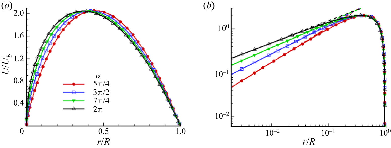
The velocity profiles along the line of symmetry  ${\theta } = 0$ are given in figure 5(a). The same profiles in a double logarithmic representation, demonstrating the validity of the approximations (2.6), are shown in figure 5(b). The maximum value of
 $U / U_b$ is approximately
 $2.05$ in all cases presented. The maximum point of
 $U / U_b$ shifts towards the apex corner from
 $r / R = 0.443$ at
 ${\alpha } = 5 {\rm \pi}/ 4$ to
 $r / R = 0.369$ at
 ${\alpha } = 2 {\rm \pi}$.
Velocity field  $U / U_b$ at several values of the apex angle
 ${\alpha }$: (a)
 ${\alpha }=5{\rm \pi} /4$, (b)
 ${\alpha }=3{\rm \pi} /2$, (c)
 ${\alpha }=7{\rm \pi} /4$, (d)
 ${\alpha }=2{\rm \pi}$.

Velocity profiles  $U / U_b$ along the line of symmetry
 ${\theta } = 0$. Dashed lines are approximations (2.6) for
 $r \to 0$.

The law of resistance  $C_f = 2 \tau _{w0} / (\rho U_b^2)$ can be derived from (2.4). Here,
 $\tau _ {w0} = - 0.25D_H\,{\rm d}P/{{\rm d}\kern0.7pt x}$ is the mean shear stress on the wall,
 $Re_H = \rho U_bD_H / \mu$ is the Reynolds number,
 $D_H = 2R {\alpha } / ({\alpha } + 2)$ is the hydraulic diameter, and
 $\rho$ is fluid density. For laminar flows in straight pipes, the friction coefficient
 $C_f$ is inversely proportional to the Reynolds number. Thus the product
 $P_O = Re_H\,C_f$, which is called the Poiseuille number, is constant with respect to the change in the Reynolds number. Determining the value of the number
 $P_O=P_O({\alpha })$ fully defines the law of resistance. Simple transformations and using (2.4) give an expression for the Poiseuille number:
 \begin{equation} P_O({\alpha})=\frac{{\rm \pi}^2{\alpha}^2}{2({\alpha}+2)^2G}. \end{equation}
The sum (2.5) can be found exactly for some values of  ${\alpha }$. In particular, if
 ${\alpha }$ is a multiple of
 ${\rm \pi}$, then (2.5) by simple manipulations is reduced to the sum of inverse squares
 $1+2^{-2}+3^{-2}+\cdots ={\rm \pi} ^2/6$. In the range of
 ${\alpha }$ in which we are interested, we get
 $G ({\rm \pi} ) = {\rm \pi}^2 / 16-1 / 2$ and
 $G (2 {\rm \pi}) = {\rm \pi}^2 / 16-4 / 9$. From this, the values of the Poiseuille number for these
 ${\alpha }$ are found:
 \begin{align} P_O({\rm \pi})=\frac{{\rm \pi}^4}{\left(\dfrac{{\rm \pi}^2}{8}-1\right)({\rm \pi}+2)^2}\approx15.77,\quad P_O(2{\rm \pi})=\frac{{\rm \pi}^4}{\left(\dfrac{{\rm \pi}^2}{8}-\dfrac{8}{9}\right)({\rm \pi}+1)^2}\approx16.47 . \end{align}
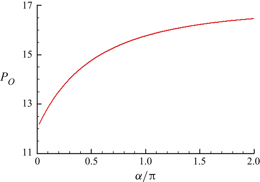
The dependence of the Poiseuille number on  ${\alpha } \in (0,2 {\rm \pi}]$ is shown in figure 6. The value of
 $P_O$ increases monotonically from
 $P_O = 12$ at
 ${\alpha } \to 0$ up to
 $P_O \approx 16.47$ for
 ${\alpha } = 2 {\rm \pi}$. Recall that in a round pipe,
 $P_O = 16$. In the pipes under consideration, the value
 $P_O =16$ is reached at
 ${\alpha } \approx 1.21{\rm \pi}$. Thus it can be said that the flows in pipes at
 ${\alpha } <1.21{\rm \pi}$ have less resistance than the flow in a round pipe at the same values of hydraulic diameter and Reynolds number. On the contrary, flows in pipes at
 ${\alpha } >1.21{\rm \pi}$ under the same conditions have greater resistance.
Dependence of the Poiseuille number on the apex angle  ${\alpha }$.

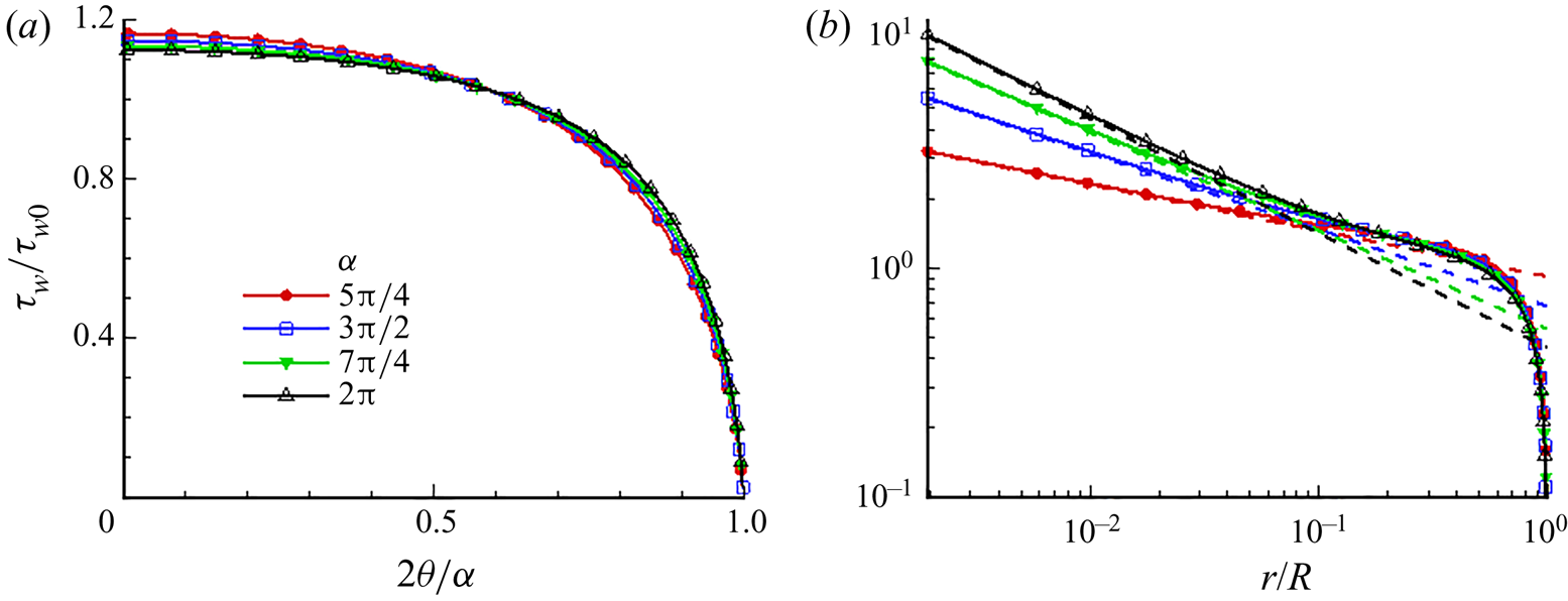
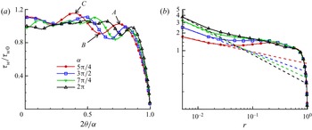
Shear stress distribution along the round part of the pipe boundary on the segment  $0 \leqslant {\theta } \leqslant {\alpha } / 2$ in pipes with apex angle
 ${\alpha }$ equal to
 $5 {\rm \pi}/ 4$,
 $3 {\rm \pi}/ 2$,
 $7 {\rm \pi}/ 4$ and
 $2 {\rm \pi}$ are shown in figure 7(a). Similar distributions along the radial boundary are shown in figure 7(b). From (2.2a,b) and (2.3), the expressions for the shear stress on the radial boundary in the vicinity of the corner point
 $r = 0$ are derived. In the internal corners,
 ${\alpha } <{\rm \pi}$, the friction at the apex corner tends to zero. It can be shown that for sufficiently large
 ${\alpha }> {\rm \pi}/ 2$,
 \begin{equation} \frac{\tau_w}{\tau_{w0}}\approx \frac{8(\alpha+2)}{4\alpha^2-{\rm \pi}^2}\left(\frac{r}{R}\right)^{{\rm \pi}/\alpha-1}. \end{equation}
At  ${\alpha } = {\rm \pi}$, the actual corner at the point
 $r = 0$ disappears, which is reflected in the fact that the shear stress acquires a finite value
 $\tau _w / \tau _ {w0} = 8 ({\rm \pi} + 2) / (3 {\rm \pi}^ 2) \approx 1.4$. In the vicinity of the external corner, for
 ${\alpha }> {\rm \pi}$, the shear stress tends to infinity, having an integrable singularity at the point
 $r = 0$. The greatest growth of
 $\tau _w \sim r^{-1/2}$ is attained for
 ${\alpha } = 2 {\rm \pi}$.
Distribution of shear stress  $\tau _w / \tau _{w0}$ along (a) the round boundary
 $\{r=R,\ 0\leqslant {\theta }\leqslant {\alpha }/2\}$ of the pipe, and (b) along the radial boundary
 $\{0< r\leqslant R,\ {\theta }={\alpha }/2\}$. Dashed lines are approximations (2.9) for
 $r \to 0$.

3. Turbulent flow in a circular-sector pipe
3.1. Formulation of the problem and method of solution
Simulation of turbulent flows is performed in traditional formulation for direct numerical simulations of turbulent flows in straight pipes and channels. The Navier–Stokes equations for incompressible fluid,
 \begin{equation} \frac{{\partial} \boldsymbol{u}}{{\partial} t}+(\boldsymbol{u}\boldsymbol{\cdot}\boldsymbol{\nabla})\boldsymbol{u}={-}\boldsymbol{\nabla} p+\nu\,\nabla^2\boldsymbol{u},\quad \boldsymbol{\nabla}\boldsymbol{\cdot}\boldsymbol{u}=0, \end{equation}
are solved with the periodicity condition along the flow and the no-slip conditions on the pipe walls. Here,  $\boldsymbol {u}$ is the velocity field,
 $p$ is the kinematic pressure, and
 $\nu$ is the kinematic viscosity. The numerical solution is carried out in polar cylindrical coordinates
 $(x, r, {\theta })$. The algorithm of Nikitin (Reference Nikitin2006b) is used, which combines a finite-difference conservative method of the second order of approximation in space and a semi-implicit scheme of the third order of integration in time (Nikitin Reference Nikitin2006a). The bulk flow rate
 $U_b$ is kept constant over time. The velocity components in polar coordinates
 $(x, r, {\theta })$ are denoted below as
 $u = U + u'$,
 $v_r = V_r + v'_r$ and
 $v_{\theta } = V_{\theta } + v'_{\theta }$.
The main series of calculations was carried out for the apex angle  ${\alpha } = 5 {\rm \pi}/ 4$,
 $3 {\rm \pi}/ 2$,
 $7 {\rm \pi}/ 4$ and
 $2 {\rm \pi}$ at the Reynolds number
 $Re = RU_b / \nu = 2000$. The Reynolds number
 $Re_H$ based on the hydraulic diameter for the listed
 ${\alpha }$ is
 $2650$, 2808, 2933 and
 $3034$, respectively. The calculations were carried out in a computational domain with length
 $10R$ on a grid of
 $128 \times 96 \times 128$ points in the
 $x, r, {\theta }$ directions, respectively. The mesh is stretched in both radial and angular directions to ensure higher resolution near rigid walls as well as near the apex corner. At the considered low Reynolds number, this grid is sufficient to resolve the main scales of turbulent motion, especially in the external corner region, which is the main object of attention in this work. The fining and even some coarsening of the computational grid do not lead to qualitative changes in the solutions presented in this paper. To determine the dependence of the flow characteristics on the Reynolds number, another simulation was carried out for a larger Reynolds number
 $Re = 4000$ (
 $Re_H = 5616$) and
 ${\alpha } = 3 {\rm \pi}/ 2$. This simulation was performed in a region of
 $6R$ length on a
 $128 \times 192 \times 256$ grid, thus preserving approximately the same (compared to the
 $Re=2000$ case) length of the computational domain and grid steps in all directions when expressed in viscous units.
Starting from some random initial conditions, the problem is integrated in time until the solution reaches a statistically steady state. After that, the equations are integrated further in time with the parallel collection of statistics. Time averaging continues for several thousand units of time  $R/U_b$ until the main mean quantities are reliably established. Along with averaging over time, averaging is carried out over the homogeneous longitudinal coordinate
 $x$, as well as over two symmetric pipe halves. In what follows, all quantities are presented in dimensionless form. The length scale is the pipe radius
 $R$, and the velocity scale is the bulk velocity
 $U_b$. Normalization by viscous scales of velocity
 $u_\tau = \sqrt {\tau _{w0} / \rho }$ and length
 $l_\tau = \nu / u_\tau$, where
 $\tau _{w0}$ is the mean wall shear stress (averaged over time and the entire pipe wall surface), is denoted by superscript
 $^+$.
The friction Reynolds number  $Re_\tau = R^+$ in the turbulent flow regime is approximately
 $140$ at
 $Re = 2000$ (at all
 ${\alpha }$) and
 $270$ at
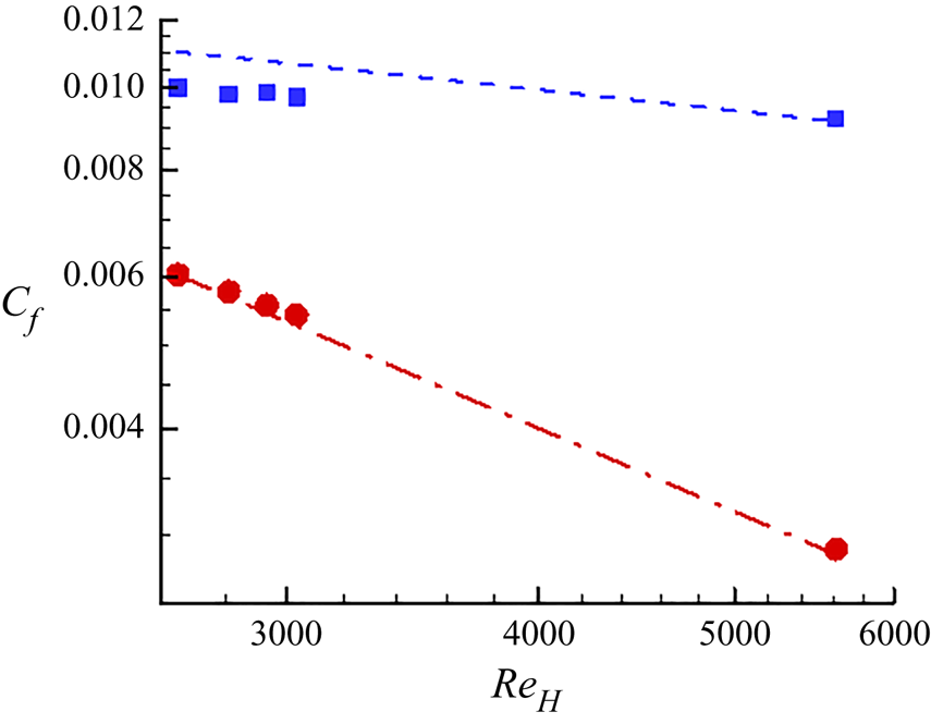
 $Re = 4000$. The friction coefficient (figure 8) increases noticeably in comparison with the laminar regime. The growth in
 $C_f$ at
 $Re = 2000$ is from 65 % at
 $\alpha = 5 {\rm \pi}/ 4$ to 80 % at
 $\alpha = 2 {\rm \pi}$. However, at this small Reynolds number, the values of
 $C_f$ turn out to be 8–9 % lower than the predictions of Blasius law for straight pipes of arbitrary cross-section:
 $C_f = 0.0791 / Re_H^{0.25}$. Perhaps this is due to the fact that at
 $Re = 2000$ the flow is not fully developed turbulent, since for the larger
 $Re$, the deviation from the Blasius law is less than 1 %.
Friction coefficient  $C_f(Re_H)$ in laminar
 $C_f=P_O({\alpha })/Re_H$ (circular symbols) and turbulent (square symbols) flows. The dashed line is from the Blasius law
 $C_f=0.0791/Re_H^{0.25}$. The dot-dashed line is from the Poiseuille law
 $C_f=16/Re_H$ for laminar circular pipe flow.

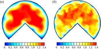
Instantaneous visualizations of the streamwise velocity in the cross-sectional plane at  ${\alpha }=3{\rm \pi} /2$, and two various Reynolds numbers, are shown in figure 9. Significant differences are noticed between the two cases. The higher
 $Re$ case exhibits formation of turbulent structures and significant scale separation between the core and the near-wall region, whereas in the lower
 $Re$ flow scale, separation is less visible. The requirements to obtain a turbulent flow in a square duct were investigated numerically by Uhlmann et al. (Reference Uhlmann, Pinelli, Kawahara and Sekimoto2007), who found that the minimum
 $Re_H$ required to sustain turbulence is
 $2154$. At this Reynolds number
 $Re_\tau \approx 77$, which means that the width of the square duct is
 $W^+\approx 154$, which ensures that at least one high-velocity streak is located on each corner, with a low-velocity streak at the duct centreplane. As argued by Uhlmann et al. (Reference Uhlmann, Pinelli, Kawahara and Sekimoto2007), this is the bare minimum for turbulence to be sustained, and therefore they denoted this state as ‘marginally turbulent’. In a circular-sector pipe, the span of the radial sections of the border is
 $Re_\tau$, which at
 $Re = 2000$ (
 $Re_\tau \approx 140$) falls somewhat short of the threshold value for sustaining turbulence in this part of the border. This is reflected in the fact that hardly one low-velocity streak is observed near the radial boundaries in figure 9(a). At
 $Re = 4000$ (
 $Re_\tau \approx 270$), the span of the radial boundaries is sufficient to form at least three low-velocity streaks on each of them (figure 9b); that is, these sections of the boundary will make a full contribution to the production of turbulence. In contrast to a square duct in a circular-sector pipe at
 ${\alpha } > {\rm \pi}$, the length
 $L_r = {\alpha } R$ of the round part of the boundary exceeds significantly the threshold of self-sustaining turbulence even at
 $Re = 2000$. For
 ${\alpha }=3{\rm \pi} /2$,
 $L_r^+\approx 660$ at
 $Re=2000$, and
 ${\approx }1270$ at
 $Re=4000$. As a result, a noticeable number of high/low-velocity regions that are commonly associated with the phenomenon of turbulence production are observed near the circular part of the boundary at
 $Re =2000$, and twice as many at
 $Re=4000$.
Instantaneous streamwise velocity at (a)  $Re=2000$, (b) and 4000, where
 ${\alpha }=3{\rm \pi} /2$.

3.2. Mean flow field
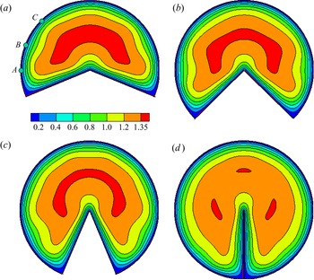
Figure 10 shows mean velocity distributions  $U (r,{\theta })$ obtained in the four described variants at
 $Re = 2000$. Mean velocity profiles along the
 ${\theta } = 0$ line are shown in figure 11. The maximum value of
 $U$ in all cases is about
 $1.4$, decreasing monotonically from
 $1.387$ at
 ${\alpha } = 5 {\rm \pi}/ 4$ to
 $1.354$ at
 ${\alpha } = 2 {\rm \pi}$. The point of maximum mean velocity is located at a greater distance from the corner than in the laminar flow (figure 5) and moves away from
 $r = 0.526$ at
 ${\alpha } = 5 {\rm \pi}/ 4$ up to
 $r = 0.572$ at
 ${\alpha } = 2 {\rm \pi}$.
Mean velocity distributions  $U (r, {\theta })$ at
 $Re = 2000$ and different values of the apex angle
 ${\alpha }$. Points
 $A$,
 $B$ and
 $C$ are the local wall friction extrema closest to the corner point
 $r = 1$,
 ${\theta } = {\alpha } / 2$.

Mean velocity profiles  $U(r)$ along the symmetry line
 ${\theta } = 0$.

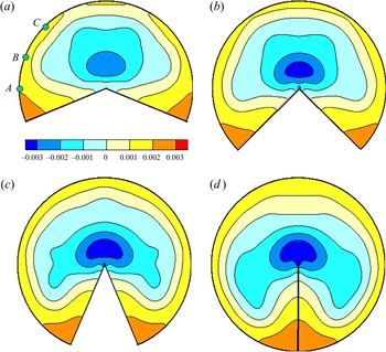
The characteristic features of the mean velocity distributions over the pipe cross-section are largely determined by the secondary flows, the streamlines of which for flows at  $Re = 2000$ are shown in figure 12. The secondary flow streamlines are the isolines of the stream function
 $\varPsi$, the fields of which are represented in figure 12 by colour contours. The stream function is defined by equations
 $rV_r={\partial }\varPsi /{\partial }{\theta },\ V_{\theta }=-{\partial }\varPsi /{\partial } r$ and
 $\varPsi =0$ on the pipe wall. Isolines of
 $\varPsi =\pm 0.0005n$,
 $n=1,2,\ldots$, are shown in figures 12 and 13(b). Solid streamlines and positive
 $\varPsi$ correspond to counterclockwise rotation of the fluid, while dashed streamlines and negative
 $\varPsi$ correspond to clockwise rotation. In this paper, a blue-green-red colour scheme is adopted for illustrating quantities exhibiting values all of equal sign (as in figure 10), while a blue–white–red colour scheme is adopted for quantities exhibiting a mean of zero (as is the case for figure 12). The mean velocity distribution and secondary flow streamlines at
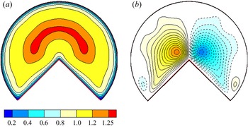
 $Re = 4000$ are shown in figure 13. The main elements of secondary flows in all considered pipes are the fluid flow towards the internal corners (points
 $r = 1$,
 ${\theta } = \pm {\alpha } / 2$), with spreading along the solid walls, and inflow along the walls to the external corner (
 $r = 0$), with ejection into the central part of the pipe along the bisector
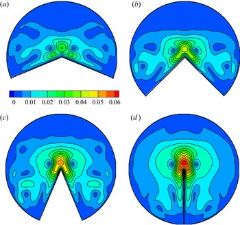
 ${\theta } = 0$. Both of these elements of the secondary flow are described generally by the mechanisms shown schematically in figure 2. The distributions of secondary flow velocity modulus at
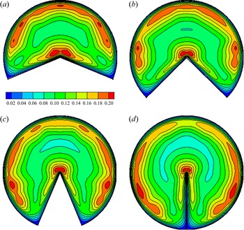
 $Re = 2000$ are shown in figure 14. The maximum of secondary flow velocity near the internal corners in all pipes is about
 $0.014$. The secondary flow velocity in the vicinity of the external corner is much higher. Its maximum is reached on the line
 ${\theta } = 0$ and increases with
 ${\alpha }$ from
 $0.03$ at
 ${\alpha } = 5{\rm \pi} /4$, to
 $0.063$ at
 ${\alpha } = 2 {\rm \pi}$. With an increase in
 $Re$, the velocity of the secondary flow also increases. At
 $Re = 4000$, it reaches
 $0.023$ in the vicinity of the internal corner, and
 $0.056$ on the line
 ${\theta } = 0$.
Secondary flows at  $Re=2000$ and different values of the apex angle
 ${\alpha }$. Points
 $A$,
 $B$ and
 $C$ are the local wall friction extrema closest to the corner point
 $r = 1$,
 ${\theta } = {\alpha } / 2$.

Mean velocity distribution (a) and secondary flows (b) at  $Re=4000$.

Distributions of secondary flow velocity modulus  $(V_r^2+V_{\theta }^2)^{0.5}$ at
 $Re = 2000$.

Secondary flows cause characteristic distortions in the mean velocity distributions: the bulges of the isolines towards the internal corners, and vice versa, towards the centre of the pipe from the external corner. Less noticeable specific details in the  $U(r,{\theta })$ distributions are revealed from the analysis of the local friction
 $\tau _w$ along the pipe walls. Figure 15 shows the graphs of
 $\tau _w / \tau _{w0}$ along the round (
 $r = 1$) and straight (
 ${\theta } = {\alpha } / 2$) sections of the pipe perimeter. As in laminar flow, the local shear stress along the radial boundary has an integrable singularity
 $\tau _w \sim r^{{\rm \pi} / {\alpha }-1}$ at
 $r \to 0$. In the vicinity of the internal corner
 $r = 1$,
 ${\theta } = \pm {\alpha }/2$, wall friction tends to zero. There are noticeable oscillations in
 $\tau _w({\theta })$ along the circular part of the boundary, especially pronounced near the corner point. The variation in
 $\tau _w$ along the circular part of the boundary and the corresponding variation in the gradient of the mean velocity
 ${\rm d}U / {\rm d}r$ is reflected in the
 $U (r,{\theta })$ distributions shown in figure 10. With distance from the corner point along the arc
 $r = 1$, two pronounced maxima
 $| {\rm d}U / {\rm d}r |$ are observed, which are separated by a point of local minimum. In figure 10(a) these extrema are marked by points
 $A$,
 $B$ and
 $C$. Similar extrema
 $|{\rm d}U /{\rm d}r |$ can be traced at all other
 ${\alpha }$.
Local wall friction  $\tau _w/\tau _{w0}$ along the round (a) and radial (b) sections of the pipe perimeter at
 $Re=2000$. Dashed lines are approximations
 ${\sim } r^{{\rm \pi} /{\alpha }-1}$ at
 $r\to 0$. Points
 $A$,
 $B$ and
 $C$ are the local wall friction extrema marked in figures 10(a) and 12(a).

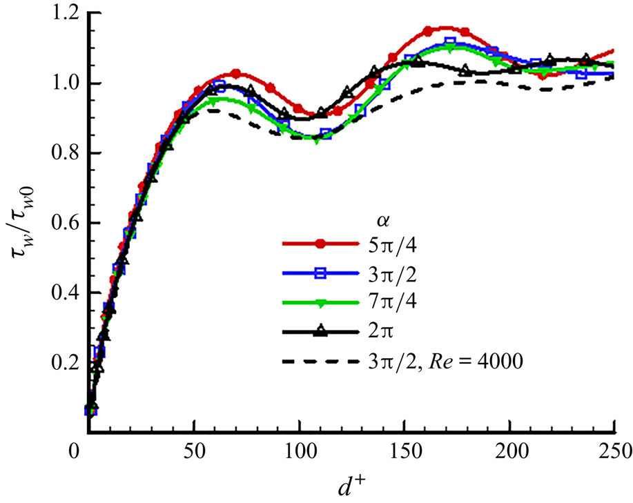
In figure 16, the change in the local friction along the circular boundary is presented as a function of the distance  $d^+ = R^+ ({\alpha } / 2- {\theta })$ from the corner point. Distributions are shown for all five calculated cases. The first maximum (corresponding to point
 $A$ in figure 10a) is located at distance
 $d^+ \approx 60$, the first minimum (point
 $B$) is at distance
 $d^+ \approx 110$, and the second maximum (point
 $C$) is at distance
 $d^+ \approx 170$. The presence of oscillations in the
 $\tau _w (d)$ distributions, and the values of
 $d^+$ at the corresponding extremum points, agree with the results of simulations of flows in square ducts (Gavrilakis Reference Gavrilakis1992; Huser & Biringen Reference Huser and Biringen1993; Pinelli et al. Reference Pinelli, Uhlmann, Sekimoto and Kawahara2010; Pirozzoli et al. Reference Pirozzoli, Modesti, Orlandi and Grasso2018). These oscillations are caused by a change in the direction of secondary flows near the boundary, which can be seen in figure 12, and especially in distributions of the mean longitudinal vorticity
 $\varOmega _x(r,{\theta })$ shown in figure 17.
Local friction  $\tau _w / \tau _{w0}$ along the round boundary of the pipe as a function of the distance
 $d^+$ from the angle
 ${\theta } = {\alpha } / 2$.

Mean longitudinal vorticity  $\varOmega _x$ distributions at
 $Re = 2000$ and different values of the angle
 ${\alpha }$. Negative values are shown by dashed lines. Points
 $A$,
 $B$ and
 $C$ are the local wall friction extrema closest to the corner point
 $r = 1$,
 ${\theta } = {\alpha } / 2$.

The coordinates of the first extrema  $\tau _w (d^+)$ and extrema of
 $\varOmega _x(r, {\theta })$ on the boundary are approximately constant in viscous units as the Reynolds number changes. On the basis of this fact, Pinelli et al. (Reference Pinelli, Uhlmann, Sekimoto and Kawahara2010) speculated that secondary flows in square ducts might be the result of the transformation of organized structures observed in near-wall turbulent flows. As can be seen from figures 12 and 17, at points
 $B$ and
 $C$, the direction of the secondary flow velocity changes. At the point
 $B$, the fluid comes along the wall and goes into the outer flow; at the point
 $C$, on the contrary, the fluid comes from the outer flow and spreads along the wall. Thus at these points, the pictures shown in figures 1(a) and 1(b) are realized, respectively. According to Nikitin (Reference Nikitin2021), a local minimum and a local maximum of the mean pressure should be reached at points
 $B$ and
 $C$. The pressure distributions
 $P (r, {\theta })$ over the pipe cross-section at
 $Re = 2000$ are shown in figure 18. The pressure in an incompressible fluid is determined to within an arbitrary additive constant. In this paper, an additional condition is adopted of a zero mean value of
 $P$ over the pipe section. In accordance with the qualitative mechanisms of the formation of secondary flows in the vicinity of the internal and external corners shown in figure 2, there is an increase in pressure in the vicinity of the internal corners
 $r = 1$,
 ${\theta } = \pm {\alpha } / 2$ and a decrease in pressure in the vicinity of the external corner
 $r = 0$.
Mean pressure distributions  $P (r, {\theta })$ at
 $Re = 2000$ and different values of
 ${\alpha }$. Points
 $A$,
 $B$ and
 $C$ are the local wall friction extrema closest to the corner point
 $r = 1$,
 ${\theta } = {\alpha } / 2$.

Figure 19 shows pressure variations along the round and radial boundaries of the pipe for all considered cases. On the round part of the boundary at distances  $d^+ \approx 110$ and
 $d^+\approx 160$ from the corner
 $r=1$,
 ${\theta }={\alpha }/2$, which correspond to points
 $B$ and
 $C$ in figure 18(a), there are local pressure extrema at
 $Re = 2000$. At the higher
 $Re$, local extrema at these points disappear, although the rate of pressure variation at these points also undergoes some changes. In Nikitin (Reference Nikitin2021), it is hypothesized that the reason for the change in pressure along the perimeter of the pipe may be a change in the curvature of the boundary. In the case under consideration, the curvature of the boundary along the arc
 $r = 1$ does not change, hence the non-monotonic change in pressure is caused by other reasons. A possible reason is the effect of near-wall turbulent structures, which confirms the hypothesis put forward in Pinelli et al. (Reference Pinelli, Uhlmann, Sekimoto and Kawahara2010) about the connection of near-wall turbulent structures with secondary flows at distances
 $d^+ = 100\text {--}200$ from the corner.
Mean pressure variation along the round boundary (a) and along the radial boundary (b).

3.3. Intensities of turbulent fluctuations
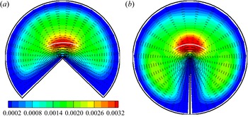
Figures 20 and 21 show the root-mean-square (r.m.s.) intensities of longitudinal  $u'_{rms}$ and transverse
 $(v'^2_{r, rms} + v'^2_{{\theta }, rms})^{0.5}$ velocity fluctuations at
 $Re = 2000$. At
 $Re = 4000$, distributions of r.m.s. intensities as a whole do not undergo significant changes, either qualitatively or quantitatively. The maximum amplitude of longitudinal fluctuations at all values of
 ${\alpha }$ is concentrated in the near-wall region along the round part of the boundary, as well as in a limited region near the external corner. The concentration of longitudinal fluctuations in the near-wall region corresponds to the typical picture of turbulent flow along a smooth wall. The maximum values of
 $u'_{rms}$ reach here
 $\approx 0.2$, which corresponds to
 $u'^+_ {rms} = u'_{rms} Re / Re_\tau \approx 2.86$, which is close to the maximum values of
 $u'^+_ {rms}$ in canonical near-wall turbulent flows. The maximum longitudinal fluctuations are located at distance
 $d \approx 0.1$ or
 $d^+ = d\,Re_\tau \approx 14$ from the wall, which also corresponds to near-wall turbulence. It is interesting that with the exception of the close proximity to the corners, the shapes of the
 $u'_{rms}$ isolines have some similarity to the isolines of the mean velocity (figure 10). This suggests that both of these quantities are subject to the convective effect of secondary flows. At maximum values of
 ${\alpha }$, when secondary flows with a noticeable amplitude capture the entire pipe cross-section (figure 12), their action leads, in particular, to the sweeping out of longitudinal fluctuations from the near-wall region near the axis of symmetry (
 ${\theta } = 0$) towards the corner regions (
 ${\theta } = \pm {\alpha } / 2$). The same effect is probably associated with a lower intensity of longitudinal fluctuations along the radial boundaries where less intense fluctuations from the corner regions are convected. The relationship between transverse fluctuations and secondary flow is less noticeable, although the characteristic deformation of the isolines towards the lower corners is also visible in figures 21(c,d). The maximum amplitude of transverse fluctuations increases monotonically from
 $0.085$ at
 ${\alpha } = 5 {\rm \pi}/ 4$, to
 $0.10$ at
 ${\alpha } = 2 {\rm \pi}$.
Distributions of the r.m.s. amplitude of longitudinal velocity fluctuations  $u'_{rms}$ at
 $Re = 2000$ and different values of
 ${\alpha }$.

Distributions of the r.m.s. amplitude of the transverse velocity fluctuations  $(v'^2_{r,rms} + v'^2_{{\theta },rms})^{0.5}$ at
 $Re = 2000$ and different values of
 ${\alpha }$.

The largest transverse fluctuations are concentrated in a well-defined area above the external corner at a distance  $r \sim 0.2$ from it. Both radial and azimuthal r.m.s. velocity fluctuations have similar distributions above the external corner, and reach 60 % and 80 %, respectively, of the r.m.s. transverse fluctuations. Significant longitudinal fluctuations are also observed above the corner, but the area of their localization is located closer to the corner point on both sides of the bisector. All this indicates that in addition to the mechanism of near-wall turbulence, the flows under consideration may also have another mechanism for generating fluctuations. Such a mechanism can be the linear instability of the mean flow, which is absent in canonical near-wall flows, such as the round pipe flow, as an example. To investigate this possibility, we studied the development of small perturbations against the background of mean flows obtained in simulations at
 $Re = 2000$. The linearized Navier–Stokes equations
 \begin{equation} \frac{{\partial} \tilde{\boldsymbol{u}}}{{\partial} t}+(\boldsymbol{U}\boldsymbol{\cdot}\boldsymbol{\nabla})\tilde{\boldsymbol{u}}+(\tilde{\boldsymbol{u}}\boldsymbol{\cdot}\boldsymbol{\nabla})\boldsymbol{U}={-}\boldsymbol{\nabla} \tilde{p}+\nu\,\nabla^2\tilde{\boldsymbol{u}},\quad \boldsymbol{\nabla}\boldsymbol{\cdot}\tilde{\boldsymbol{u}}=0, \end{equation}
are solved for perturbations of the form  $\tilde {\boldsymbol {u}}(t,x,r,{\theta }) = \hat {\boldsymbol {u}}(t,r,{\theta })\exp ({\rm i}\beta x)$ with some random initial conditions. The mean velocity field
 $(U, V_r, V_{\theta })$ is taken as the main flow
 $\boldsymbol {U} (r,{\theta })$. Integration over time continues until the solution reaches the asymptotic exponential behaviour
 $| \hat {\boldsymbol {u}}(t, r,{\theta }) | \sim \exp \lambda t$, which corresponds to the behaviour of the fastest growing (or least decaying) eigenfunction of operator (3.2a,b). If it turns out that
 $\lambda > 0$, then this means the instability of the main flow to perturbations with a given wavenumber
 $\beta$; otherwise, the flow is stable.
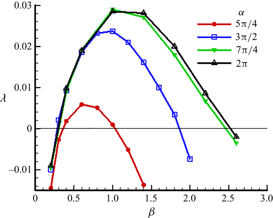
The calculations performed have shown the instability of mean flows at all values of  ${\alpha }$. The dependence of the growth coefficient
 $\lambda$ of the most growing perturbations on the wavenumber
 $\beta$ is shown in figure 22. The degree of flow instability increases with
 ${\alpha }$, the maximum values of
 $\lambda$ increase, and the range of wavenumbers of unstable perturbations expands. This behaviour is consistent with a slight increase in the amplitude of transverse fluctuations with an increase in
 ${\alpha }$ (figure 21).
Dependence of the growth coefficient of small perturbations  $\lambda$ on the wavenumber
 $\beta$ at
 $Re = 2000$ and different values of
 ${\alpha }$.

As expected, the growing perturbations in all cases are concentrated in the region above the external corner. Figure 23 shows the intensity distributions of longitudinal and transverse velocity fluctuations of the most rapidly growing perturbations ( $\beta = 1.0$) in a pipe with angle
 ${\alpha } = 3 {\rm \pi}/ 2$. The intensity of the longitudinal fluctuations is four times the intensity of the transverse fluctuations. Isolines in figure 23 are shown against the background of the mean velocity distribution. The distribution of longitudinal fluctuations (with zero values on the symmetry line
 ${\theta } = 0$) corresponds to the sinous type of instability. The distribution of radial fluctuations has a similar symmetry (not shown in the figure). The distribution of angular velocity fluctuations has the opposite symmetry corresponding to the condition
 ${\partial } / {\partial }{\theta } = 0$ at
 ${\theta } = 0$. The distributions of the longitudinal and transverse velocity fluctuations shown in figures 20 and 21 differ in detail from similar distributions for growing linear perturbations. What is important, however, is a qualitative agreement, consisting of the location of both in the area above the external corner. The latter allows us to hypothesize that noticeable anomalies in the distribution of the intensity of velocity fluctuations in the region above the external corner in the considered turbulent flows are caused by the instability of the mean flow to small perturbations.
Isolines of the amplitude of the longitudinal (a) and transverse (b) fluctuations of the fastest-growing perturbation ( $\beta = 1$) against the background of the mean velocity distribution
 $U (r, {\theta })$ at
 ${\alpha } = 3 {\rm \pi}/ 2$. The intensity of the longitudinal fluctuations is four times the intensity of the transverse fluctuations.

3.4. Formation of secondary flows
Secondary flow is described by the set of Reynolds equations
 \begin{gather} V_r\,\frac{{\partial} V_r}{{\partial} r}+\frac{1}{r}\,V_{\theta}\,\frac{{\partial} V_r}{{\partial}{\theta}}-\frac{V_{\theta}^2}{r}+\frac{1}{Re}\,\frac{1}{r}\,\frac{{\partial}\varOmega_x}{{\partial}{\theta}}+\frac{{\partial} P}{{\partial} r}={-}\frac{{\partial}\overline{v'^2_r}}{{\partial} r}-\frac{1}{r}\,\frac{{\partial}\overline{v'_rv'_{\theta}}}{{\partial}{\theta}}+\frac{\overline{v'^2_{\theta}}-\overline{v'^2_r}}{r}\equiv F_r, \end{gather}
 \begin{gather}V_r\,\frac{{\partial} V_{\theta}}{{\partial} r}+\frac{1}{r}\,V_{\theta}\,\frac{{\partial} V_{\theta}}{{\partial}{\theta}}+\frac{V_rV_{\theta}}{r}-\frac{1}{Re}\,\frac{{\partial}\varOmega_x}{{\partial} r}+\frac{1}{r}\,\frac{{\partial} P}{{\partial}{\theta}}={-}\frac{{\partial}\overline{v'_rv'_{\theta}}}{{\partial} r}-\frac{1}{r}\,\frac{{\partial}\overline{v'^2_{\theta}}}{{\partial}{\theta}}-\frac{2\overline{v'_rv'_{\theta}}}{r}\equiv F_{\theta}, \end{gather}
 \begin{gather}\frac{1}{r}\,\frac{{\partial} rV_r}{{\partial} r}+\frac{1}{r}\,\frac{{\partial} V_{\theta}}{{\partial}{\theta}}=0,\quad \varOmega_x=\frac{1}{r}\,\frac{{\partial} rV_{\theta}}{{\partial} r}-\frac{1}{r}\,\frac{{\partial} V_r}{{\partial}{\theta}} . \end{gather}
In rectilinear flows, secondary flows are uniquely related to the mean longitudinal vorticity  $\varOmega _x$; therefore the analysis of the causes and conditions for the occurrence of secondary flows in most previous works was carried out from the standpoint of studying the mechanisms of generation of
 $\varOmega _x$, which are described by (1.1). This equation does not contain pressure, which makes it potentially more convenient for analysis compared to the equivalent set of Reynolds equations (3.3)–(3.5a,b). The production of
 $\varOmega _x$ is described by the source term
 $S$ on the right-hand side of (1.1), which in turn is expressed in terms of the second derivatives of the Reynolds stresses (1.2). As noted in the Introduction, splitting the expression (1.2) into terms
 $S_1, S_2$ corresponding to normal and shear Reynolds stresses is not very promising, since these quantities are not invariants and therefore have no definite physical meaning. In the considered flows near the external corner, the problem is further complicated by the fact that the corner point is a singularity point, at which infinite values of the gradients of the hydrodynamic parameters should be expected. An attempt to analyse the source term
 $S$ and its constituent terms
 $S_1, S_2$ in the vicinity of the external corner of
 $270^\circ$ was made in Xu (Reference Xu2009). It is noted that the value of
 $S$ increases by several orders of magnitude when approaching the corner point from different sides of the symmetry line. The distributions of each of the terms
 $S_1, S_2$ have a fancy shape in the form of a butterfly with three pairs of wings. Moreover, as in most other flows, the values of
 $S_1, S_2$ are close in magnitude but opposite in sign at the corresponding points. Based on these observations, it is difficult to predict the shape of the emerging secondary flows, not to mention the mechanisms of their occurrence.
In Nikitin et al. (Reference Nikitin, Popelenskaya and Stroh2021), a qualitative explanation of the cause of the secondary flow in a turbulent flow along the external corner is proposed. Secondary flow occurs as a result of the action of the centrifugal force arising during the fluctuating flow around the corner in the plane transverse to the direction of the main flow (figure 2(b) of this paper). To quantify the centrifugal force in a fluctuating flow in Nikitin (Reference Nikitin2021), the concept of a fluctuation trajectory is introduced as a line in a cross-section, the direction of the tangent to which at each point coincides with the principal direction of the Reynolds stress tensor corresponding to larger principal stress. In other words, if  $v_\tau '$ and
 $v_n'$ are tangential and normal components of velocity fluctuations on the trajectory, then
 $\overline {v_\tau '^2}> \overline {v_n'^2}$ and
 $\overline {v_\tau 'v_n'} = 0$.
The principal stresses and principal directions are defined as the eigenvalues and eigenvectors of the Reynolds stress tensor. At each point  $(r,{\theta })$ of the pipe cross-section, the components of the tangent
 ${\boldsymbol {\tau }}=(\tau _r,\tau _{\theta })$ and normal
 ${\boldsymbol {n}}=(n_r,n_{\theta })$ vectors to the fluctuation trajectory are found from the linear equations
 \begin{equation} \begin{pmatrix} \overline{v_r'^2} & \overline{v_r'v_{\theta}'} \\ \overline{v_r'v_{\theta}'} & \overline{v_{\theta}'^2} \end{pmatrix} \begin{pmatrix} \tau_r \\ \tau_{\theta} \end{pmatrix} = \overline{v_\tau'^2} \begin{pmatrix} \tau_r \\ \tau_{\theta} \end{pmatrix} , \quad \begin{pmatrix} \overline{v_r'^2} & \overline{v_r'v_{\theta}'} \\ \overline{v_r'v_{\theta}'} & \overline{v_{\theta}'^2} \end{pmatrix} \begin{pmatrix} n_r \\ n_{\theta} \end{pmatrix} = \overline{v_n'^2} \begin{pmatrix} n_r \\ n_{\theta} \end{pmatrix}, \end{equation}
where
 \begin{align} \overline{v_\tau'^2}=\frac{\overline{v_r'^2}+\overline{v_{\theta}'^2}}{2}+\sqrt{D}, \quad \overline{v_n'^2}=\frac{\overline{v_r'^2}+\overline{v_{\theta}'^2}}{2}-\sqrt{D}, \quad D=\frac{1}{4}\left(\overline{v_r'^2}-\overline{v_{\theta}'^2}\right)^2-\overline{v_r'v_{\theta}'}^2. \end{align}
It is assumed that  $\boldsymbol {n}$ is the vector opposite to the main normal vector, that is, directed towards the convexity of the trajectory. It is shown in Nikitin (Reference Nikitin2021) that the Reynolds-stress force
 $F_n$ acting in the
 ${\boldsymbol {n}}$ direction is expressed as
 \begin{equation} F_n={-}\frac{{\partial}\overline{v_n'^2}}{{\partial} n}+\frac{\overline{v_\tau'^2}-\overline{v_n'^2}}{R_t}. \end{equation}
Here,  $R_t$ is the radius of curvature of the trajectory at the point under consideration. The first term on the right-hand side of (3.8) can have any sign. We can say that the force normal to the trajectory caused by this term is directed towards the decrease in the intensity of normal fluctuations. The second term is always positive, that is, the force corresponding to this term is directed towards the convexity of the trajectory and is proportional to its curvature
 $R_t^{-1}$. It can be interpreted as a centrifugal force.
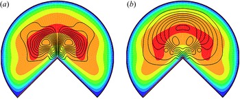
Figure 24 shows the fluctuation trajectories in pipes with apex angles  ${\alpha } = 3 {\rm \pi}/ 2$ and
 $2 {\rm \pi}$ (
 $Re = 2000$). The trajectories are represented by tangent segments at the nodes of the computational grid (every fourth node in each direction is used). The length of the tangent segments is proportional to
 $\overline {v_\tau '^2} - \overline {v_n'^2}$. The fields of
 $\overline {v_n'^2}$ are shown in figure 24 by coloured contours. These diagrams allow estimating the distributions of each term in the right-hand part of the expression (3.8) along the pipe cross-section.
Fluctuation trajectories and contours of  $\overline {v_n'^2}$ at
 $Re=2000$, for (a)
 ${\alpha }=3{\rm \pi} /2$, and (b)
 $2{\rm \pi}$. The length of the line segments is proportional to
 $\overline {v_\tau '^2}-\overline {v_n'^2}$. White curves show the location where
 ${\partial }\overline {v_n'^2}/{\partial } n$ change sign.

The centrifugal force at each point is directed towards the convexity of the trajectory; it is proportional to  $\overline {v_\tau '^2} - \overline {v_n'^2}$ (i.e. the length of the tangent segments in figure 24) and is inversely proportional to the radius of curvature of the trajectory, which can be estimated visually from the figure. The first term in (3.8) is directed along the normal to the trajectory in the direction of decreasing
 $\overline {v_n'^2}$.
Along the boundaries, the trajectories are parallel to the walls. The Reynolds-stress force  $F_n$ acts everywhere towards the wall, which causes an increase in pressure (see figure 18). At the radial boundaries, the fluctuation trajectories are rectilinear and there are no centrifugal forces. Only the first term in (3.8) is responsible for the pressure increase when approaching the radial walls. The trajectories are curvilinear along the round boundaries so that both terms in (3.8) make a positive contribution. In the vicinity of the internal corners (
 $r = 1$,
 ${\theta } = \pm {\alpha } / 2$), the trajectories are strongly curved, which generates a centrifugal force directed towards the corners. This force is noticeable in magnitude due to the large curvature of the trajectories, despite the small value of
 $\overline {v_\tau '^2} - \overline {v_n'^2}$ in this region. Together with the positive contribution of the first term, it creates a significant increase in pressure in the corner regions.
In the vicinity of the external corner, the fluctuation trajectories acquire an  $\varOmega$-shaped form, joining the straight sections along each of the two radial boundaries. When approaching the corner, the curvature of the trajectories tends to infinity, which, as will be shown below, leads to an unlimited increase in the centrifugal force directed away from the corner. Moving away from the corner, the curvature of the trajectories decreases. The difference
 $\overline {v_\tau '^2} - \overline {v_n'^2}$ decreases as well, so that the magnitude of the centrifugal force becomes small. Its effect practically disappears at half the distance to the outer wall, after which it begins to grow again approaching the curvilinear round border.
A significant contribution to the balance of forces acting along the normal to the fluctuation trajectories is made by the presence of intense transverse velocity fluctuations with a maximum in the region  $r = 0.2\text {--}0.25$ above the corner (see figure 21). As shown above, the probable cause of the appearance of intense fluctuations in this region is the linear instability of the mean flow. The intensity
 $\overline {v_n'^2}$ decreases on both sides of the maximum line at
 $r\approx 0.25$, shown by white curves in figure 24. Respectively, the force generated by the first term in (3.8) changes sign from negative at small
 $r$ to positive at the larger
 $r$.
Determining the numerical values of the components of the force  $F_n$ in (3.8) at an arbitrary point requires a rather cumbersome computational procedure. Therefore, we will limit ourselves to estimating these values along the symmetry line
 ${\theta } = 0$. The Reynolds equation along this coordinate line has the form
 \begin{gather} \underbrace{V_r\,\frac{{\partial} V_r}{{\partial} r}}_{{-}Conv}-\underbrace{\frac{1}{Re}\left(\frac{1}{r^2}\,\frac{{\partial}}{{\partial} r}r\,\frac{{\partial} rV_r}{{\partial} r}+\frac{1}{r^2}\,\frac{{\partial}^2V_r}{{\partial}{\theta}^2}\right)}_{{-}Visc}+\underbrace{\frac{{\partial} P}{{\partial} r}}_{{-}Pres}=F_r, \end{gather}
 \begin{gather}F_r=\underbrace{-\frac{{\partial}\overline{v'^2_r}}{{\partial} r}}_{F_{vr}}\underbrace{{}-\frac{1}{r}\,\frac{{\partial}\overline{v'_rv'_{\theta}}}{{\partial}{\theta}}+\frac{\overline{v'^2_{\theta}}-\overline{v'^2_r}}{r}}_{F_{cf}}. \end{gather}
The convective term on the left-hand side of (3.9) has a reduced form because the azimuthal mean-velocity component  $V_{\theta }$ is equal to zero on a symmetry line. The Reynolds-stress force
 $F_r$, which is equal to
 $F_n$ of (3.8), includes
 ${\partial }\overline {v'^2_r}/{\partial } r$, which at
 ${\theta }=0$ coincides with
 ${\partial }\overline {v'^2_n}/{\partial } n$, hence the remaining terms in (3.10) represent the centrifugal force.
Figure 25(a) shows the distributions of all terms of (3.9) and (3.10) along the line  ${\theta } = 0$ in the pipe with
 ${\alpha } = 3 {\rm \pi}/ 2$ and
 $Re = 2000$. The positive value of each of the presented quantities corresponds to the force acting on the fluid element in the positive direction of the coordinate
 $r$. The sum of all forces at each point is zero. In agreement with the qualitative estimates made, the centrifugal force
 $F_{cf}$ is positive for all
 $r$, which reflects the fact that the convexities of fluctuation trajectories that intersect the line
 ${\theta } = 0$ are directed away from the corner. At
 $r \to 0$, the centrifugal force increases, which indicates the probable singularity of
 $F_{cf}(r)$ at
 $r = 0$. The force corresponding to
 $F_{vr}$ is determined by the change in the intensity of the radial fluctuations. At
 $r <0.25$, the intensity of radial fluctuations increases, so that
 $F_{vr}$ is negative. At
 $0.1< r<0.2$, it outweights the centrifugal force, thus the Reynolds-stress force as a whole acts here towards the corner point. Further from the corner,
 $F_{vr}$ first decreases and then changes to positive. The presence of forces acting on a fluid particle in the radial direction causes a reaction in the form of a pressure change. For
 $r <0.04$, while the centrifugal force dominates, the pressure increases, and
 $- {\partial } P / {\partial } r$ is negative. For larger
 $r$, as the intensity of radial fluctuations as well as the velocity of the secondary flow increases,
 $- {\partial } P / {\partial } r$ changes sign to positive. The pressure continues to decrease with increasing
 $r$ up to
 $r = 0.2$ (coordinate of the pressure minimum point in figure 18b). Further, as the sum of the Reynolds-stress forces becomes positive, it is compensated by the negative value of
 $- {\partial } P / {\partial } r$. The main output following from the observation of the variation of various terms in (3.9) and (3.10) is that the characteristic decrease in pressure in the area above the corner point (figure 18) is due to the pressure reaction to the presence of the
 $F_{vr}$ force acting in this area towards the corner. The convective term has a pronounced value, acting first against the direction of the secondary flow, and then (at
 $r> 0.13$) along it. The viscous force is negligible all over
 ${\theta }=0$.


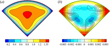
For comparison, figure 25(b) shows the distributions of all terms of (3.9) and (3.10) along the line  ${\theta } = 0$ in a pipe with internal apex angle
 ${\alpha } = {\rm \pi}/ 2$ at
 $Re_H = 2800$. Some results of simulating the turbulent flow in such a pipe are given in figure 26, which shows the mean velocity field, the pressure field, and streamlines of the secondary flow (see also Nikitin Reference Nikitin2021; Nikitin et al. Reference Nikitin, Popelenskaya and Stroh2021). In accordance with the qualitative mechanism for the formation of secondary flows in the internal corners (figure 2a), an increase in pressure occurs in each of the three corner points. The secondary flow is directed from the outer flow along the corner bisector and along the walls away from the corner. The centrifugal force
 $F_{cf}$ on the line
 ${\theta } = 0$ is negative at
 $r <0.62$, which corresponds to the convexity of the fluctuation trajectories towards the corner
 $r = 0$. However, later, near the opposite round wall, the fluctuation trajectories turn towards the wall, and the centrifugal force changes its sign to positive. The force
 $F_{vr} = - {\partial } \overline {v'^2_r} / {\partial } r$ is negative in the near-corner region and positive near the wall
 $r = 1$. This obviously corresponds to an increase and then a decay of radial velocity fluctuations. The pressure force balances the sum
 $F_ {vr} + F_ {cf}$ up to a small sum of viscous and convective forces. Viscous force is positive in the interval
 $r <0.5$ where the secondary flow velocity is directed towards the corner, that is, the viscous force acts against the motion.
Mean velocity distribution (a), and contours of mean pressure and secondary flow streamlines (b), in a pipe with apex angle  ${\alpha }={\rm \pi} /2$.

The inconvenience of using the Reynolds equations (3.3)–(3.5a,b) is due to the fact that they contain pressure, the exact distribution of which is difficult to estimate a priori. Even with the known distributions of the forces  $F_r$ and
 $F_{\theta }$, the prediction of the shape of the secondary flows caused by them is generally non-trivial since part of these forces is balanced by the pressure gradient. A gradient of an arbitrary scalar field can be added in the right-hand parts of (3.3) and (3.4), and this will not change the secondary flow, but will change the pressure distribution. Thus one can say that secondary flows are formed not by the forces
 $F_r$ and
 $F_{\theta }$ themselves, but by their vortical component.
According to the Helmholtz theorem, any sufficiently smooth vector field is decomposed into the sum of the vortical (solenoidal) and potential components. Thus the vector field of Reynolds-stress forces  ${\boldsymbol {F}} = (F_r, F_{\theta })$ can be represented as
 \begin{equation} {\boldsymbol{F}}={\boldsymbol{G}} + \boldsymbol{\nabla} q, \quad \boldsymbol{\nabla}\boldsymbol{\cdot}{\boldsymbol{G}} = 0. \end{equation}
Equations (3.11a,b) lead to the Poisson equation for the potential  $q$, and the condition of zero normal forces on the boundary
 $\varGamma$ leads to the Neumann condition. Thus we get the problem
 \begin{equation} \Delta q = \boldsymbol{\nabla}\boldsymbol{\cdot}{\boldsymbol{F}}, \quad {\partial} q/{\partial} n|_\varGamma = 0 . \end{equation}
Under these conditions, the representation (3.11a,b) is unique. It is shown in Nikitin (Reference Nikitin2021) that the vortical component  $\boldsymbol {G}$ of the Reynolds-stress forces in the vicinity of the
 $90^\circ$ corner reproduces with high accuracy the shape of the secondary flows caused by these forces.
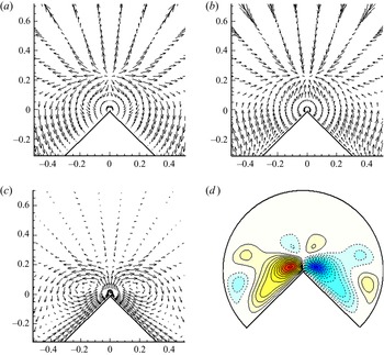
Figure 27 shows the vector fields of force  $\boldsymbol {F}$, potential force
 $- \nabla q$ and their sum
 $\boldsymbol {G}$, constructed for the flow at
 $Re = 2000$ and
 ${\alpha } = 3 {\rm \pi}/ 2$. For clarity, the area adjacent to the corner point
 $r = 0$ is shown. To eliminate large values at
 $r \to 0$, the lengths of all vectors are multiplied by
 $r$. The vector field
 $\boldsymbol {G}$ is solenoidal, which means that it is representable as a curl of the vector potential
 ${\boldsymbol {G}} = \boldsymbol {\nabla } \times A \boldsymbol {i}$ (where
 $\boldsymbol {i}$ is the unit vector along the
 $x$ axis). The scalar function
 $A$ with respect to the vector field
 ${\boldsymbol {G}}$ is analogous to the stream function
 $\varPsi$ with respect to the velocity field of the secondary flow
 $(V_r,V_{\theta })$. The vector lines of
 ${\boldsymbol {G}}$ coincide with the isolines of field
 $A$ that is shown in figure 27(d). This representation gives a more visual impression of the field
 $\boldsymbol {G}$. Visualization of the force field
 $\boldsymbol {F}$ does not give an idea of the secondary flow generated by it. A characteristic feature of this vector field is the presence of a knot-type singular point in the region
 $(r, {\theta }) = (0.2, 0)$. This point coincides with the point of the local maximum of the intensity of transverse velocity fluctuations (figure 21). The potential component
 $- \boldsymbol {\nabla } q$ is very close to the field
 $\boldsymbol {F}$, taken with the opposite sign. A significant difference concerns the near-wall layers, where the original field has a zero tangential component, and
 $- \boldsymbol {\nabla } q$ is non-zero. The sum of these two fields gives the vortical component
 $\boldsymbol {G}$, the field of which already reproduces the main qualitative features of the secondary flow in the vicinity of the external corner: the direction of vector lines along the radial walls towards the corner and from the corner upwise along the bisector. This field, however, contains a noticeable qualitative difference from the secondary flow field in the region above the external corner (figure 12). This difference consists in a change in the direction of the vector field on the line
 ${\theta } = 0$ in the region of the point
 $r = 0.2$, while the secondary flow does not change direction on the line
 ${\theta } = 0$. The reason for the unidirectional nature of the secondary flow is the action of the convective force, which, as can be seen from figure 25, in the region of
 $r = 0.2$ has the greatest positive value. In the regions adjacent to the internal corners (
 $r = 1$,
 ${\theta } = \pm {\alpha } / 2$), convective forces are insignificant, and as a consequence, the vector field
 $\boldsymbol {G}$ reproduces the shape of the secondary flow with good accuracy.
Vector fields of (a) Reynolds-stress forces  $\boldsymbol {F}$, (b) potential component
 $- \boldsymbol {\nabla } q$, and (c) vortical component
 $\boldsymbol {G}$, for
 ${\alpha } = 3 {\rm \pi}/ 2$,
 $Re = 2000$. The arrows in (c) are three times the lengths in (a,b). Panel (d) shows the vector lines of the solenoidal field
 $\boldsymbol {G}$.

4. Summary
In this work, a numerical study of turbulent flows in straight pipes with a cross-section in the form of a circular sector with different values of the apex angle  ${\alpha }$ is carried out. The main attention is paid to flows along the external corners
 ${\alpha }>{\rm \pi}$. Such flows are insufficiently described in the literature, while they have a number of interesting features.
An analytical solution for laminar flow in the geometry under consideration is presented, which differs from that obtained earlier in White (Reference White2006). The law of resistance is determined, and the distribution of the velocity  $U$ over the pipe cross-section is constructed. The main term of the asymptotics of
 $U (r)$ is calculated for
 $r \to 0$, and the singularity of the wall friction
 $\tau _w \sim r^{{\rm \pi} / {\alpha }-1}$ is shown for
 ${\alpha }> {\rm \pi}$.
Turbulent flows were simulated for  $Re = 2000$ and four values of the apex angle,
 ${\alpha } = 5 {\rm \pi}/ 4$,
 $3 {\rm \pi}/ 2$,
 $7 {\rm \pi}/ 4$ and
 $2 {\rm \pi}$. To estimate the dependence of the flow characteristics on the Reynolds number, the flow was simulated for a larger Reynolds number
 $Re = 4000$ and
 ${\alpha } = 3 {\rm \pi}/ 2$. The transition to a turbulent flow is accompanied by a noticeable increase in the friction coefficient
 $C_f$. At
 $Re = 2000$, this increase is from 65 % at
 $\alpha = 5 {\rm \pi}/ 4$, to 80 % at
 ${\alpha } = 2 {\rm \pi}$. For a larger Reynolds number, the value of
 $C_f$ agrees with 1 % accuracy with the Blasius law for pipes of arbitrary cross-section. The maximum mean velocity
 $U_m$ in all variants is about
 $1.4$ (velocities and lengths are normalized by the bulk velocity and by the pipe radius) at
 $Re = 2000$, and about
 $1.26$ at
 $Re = 4000$. This is significantly less than
 $U_m \approx 2.05$ in laminar flow.
The distributions of the mean velocity over the cross-section of the pipe have characteristic features in the form of bulges of isolines towards the internal corners of the cross-section and bulges away from the external corner in the apex of the circular sector. This behaviour of the mean velocity isolines is determined by the behaviour of the secondary flows. The main elements of secondary flows are fluid inflow to the internal corners with a corresponding spreading along the walls, and, conversely, the fluid flow towards the external corner along the radial walls with a further outflow from the corner along the bisector. The secondary flow velocity in the vicinity of the external corner at  $Re = 2000$ increases with
 ${\alpha }$ from
 $0.03$ to
 $0.063$. This is noticeably higher than the secondary flow velocity in the vicinity of internal corners, where it is about
 $0.014$ at all
 ${\alpha }$.
It is found that the wall shear stress distribution along the radial walls is qualitatively similar to that in the laminar flow with the same asymptotics  $\tau _w \sim r^{{\rm \pi} / {\alpha }-1}$ at
 $r \to 0$. On the round boundary, several fluctuations in the
 $\tau _w({\theta })$ distribution are noticeable with distance from the corner points
 ${\theta } = \pm {\alpha } / 2$. The extrema are located at points on the border, near which the secondary flow changes its direction. It is noticed that the distances along the boundary from the corner to the local maximum and minimum points of
 $\tau _w ({\theta })$ are approximately constant when normalized by viscous scales. This circumstance indicates a possible connection between secondary flows in this area with organized near-wall structures of turbulent flow (Pinelli et al. Reference Pinelli, Uhlmann, Sekimoto and Kawahara2010).
The distribution of the intensity of the longitudinal velocity fluctuations near the circular part of the cross-section perimeter as a whole corresponds to the picture of the canonical near-wall turbulent flow. The maximum value  $u'^+ \approx 2.8$ is reached at distance
 $d^+\approx 14$ from the wall. A characteristic feature of the transverse velocity fluctuation pattern is the presence of a rather sharply outlined region of intense fluctuations located above the apex of the external corner (that is, on the bisector of the corner) at distance
 $r \sim 0.2$ from it. The amplitude of transverse fluctuations here reaches half of the maximum of longitudinal fluctuations. The presence of a pronounced region with an increased level of velocity fluctuations indicates that in addition to the mechanism of generation of fluctuations in near-wall flows, an alternative mechanism, for example, a linear instability, can be present in the considered flows. To test this hypothesis, studies of the linear stability of the calculated mean flow fields at all angles
 ${\alpha }$ were carried out. It turned out that indeed, these fields are linearly unstable, and the range of wavenumbers of unstable perturbations and the characteristic growth rates of their growth increase with
 ${\alpha }$. The amplitude of the growing perturbations is concentrated in the region above the apex corner, which confirms the hypothesis about the linear instability of the flow as the cause of the formation of increased intensity of fluctuations in this region.
In this work, considerable attention is paid to the study of the features of the formation of secondary flows. In general, the emerging secondary flows fit into the qualitative mechanism formulated in Nikitin (Reference Nikitin2021) and Nikitin et al. (Reference Nikitin, Popelenskaya and Stroh2021). According to this mechanism, the main driving element that generates secondary flows is the centrifugal force arising from a transverse fluctuating flow around a corner in a turbulent flow. When flowing around the internal corner, the convexity of the curved trajectories of fluid particles, as well as the centrifugal force, are directed towards the corner. On the contrary, when flowing around the external corner, the convexity of the trajectories, and hence the centrifugal force, are directed away from the corner. These forces cannot be balanced fully by the pressure gradient, since a pressure change (pressure increase in the internal corner and a decrease in the external corner) will inevitably cause fluid movement along the surrounding walls (diverging flow from the internal corner and converging towards the external corner).
The described qualitative picture is somewhat disturbed by the presence of increased intensity of transverse velocity fluctuations in the region above the apex of the external corner. Turbulent fluctuations generate a force acting in the direction of their decreasing intensity. Thus a localized spot of intense fluctuations existing above the external corner produces a force acting in all directions from this spot, and in particular, towards the corner, that is, opposite the centrifugal force. To clarify all the details accompanying the formation of the secondary flow in this area, a detailed study of the fluctuation forces in the vicinity of the external corner was carried out. It is shown that in order to neutralize the force generated by the mentioned spot of localized fluctuations, the pressure decreases with distance from the corner along the bisector, which creates a region of minimum pressure at some distance from the apex of the corner.
The inconvenience of using the Reynolds equations to describe secondary flows is due to the fact that they contain pressure, the exact distribution of which is difficult to estimate a priori. Even knowing the distribution of the Reynolds-stress force field  $\boldsymbol {F}$, the prediction of the shape of the secondary flows caused by it is generally non-trivial since some part of this force is compensated by the pressure gradient. Continuing the line of Nikitin (Reference Nikitin2021), it is shown in this work that the vortical component of the field
 $\boldsymbol {F}$, which is calculated using the Helmholtz decomposition, reproduces to a certain extent the shape of secondary flows.
Acknowledgements
The research was carried out using the equipment of the shared research facilities of HPC computing resources at Lomonosov Moscow State University and computing resources of the federal collective usage centre Complex for Simulation and Data Processing for Mega-science Facilities at NRC ‘Kurchatov Institute’ (ministry subvention under agreement RFMEFI62117X0016), http://ckp.nrcki.ru/.
Funding
The reported study was funded by RSF, project no. 18-71-10075.
Declaration of interests
The authors report no conflict of interest.