Bifurcations and pattern formation in a host–parasitoid model with nonlocal effect

Chuang Xiang; Jicai Huang; Min Lu; Shigui Ruan; Hao Wang

doi:10.1017/prm.2024.24

Bifurcations and pattern formation in a host–parasitoid model with nonlocal effect

Part of: Qualitative theory Parabolic equations and systems

Published online by Cambridge University Press: 04 March 2024

Min Lu ,

and

Chuang Xiang: Affiliation:
School of Mathematical Sciences, Nanjing Normal University, Nanjing 210023, P. R. China (1604059603@qq.com) School of Mathematics and Statistics, Central China Normal University, Wuhan, Hubei 430079, P. R. China
Jicai Huang: Affiliation:
School of Mathematics and Statistics, Central China Normal University, Wuhan, Hubei 430079, P. R. China (hjc@ccnu.edu.cn, lumin@mails.ccnu.edu.cn)
Min Lu: Affiliation:
School of Mathematics and Statistics, Central China Normal University, Wuhan, Hubei 430079, P. R. China (hjc@ccnu.edu.cn, lumin@mails.ccnu.edu.cn)
Shigui Ruan: Affiliation:
Department of Mathematics, University of Miami, Coral Gables, FL 33146, USA (ruan@math.miami.edu)
Hao Wang: Affiliation:
Department of Mathematical and Statistical Sciences, University of Alberta, Edmonton, AB T6G 2G1, Canada (hao8@ualberta.ca)

Article contents

Abstract
Introduction
Hopf bifurcation of the ODE system
System () with local intraspecific prey competition
System () with nonlocal intraspecific prey competition
Concluding remarks
References

Rights & Permissions

Abstract

In this paper, we analyse Turing instability and bifurcations in a host–parasitoid model with nonlocal effect. For a ordinary differential equation model, we provide some preliminary analysis on Hopf bifurcation. For a reaction–diffusion model with local intraspecific prey competition, we first explore the Turing instability of spatially homogeneous steady states. Next, we show that the model can undergo Hopf bifurcation and Turing–Hopf bifurcation, and find that a pair of spatially nonhomogeneous periodic solutions is stable for a (8,0)-mode Turing–Hopf bifurcation and unstable for a (3,0)-mode Turing–Hopf bifurcation. For a reaction–diffusion model with nonlocal intraspecific prey competition, we study the existence of the Hopf bifurcation, double-Hopf bifurcation, Turing bifurcation, and Turing–Hopf bifurcation successively, and find that a spatially nonhomogeneous quasi-periodic solution is unstable for a (0,1)-mode double-Hopf bifurcation. Our results indicate that the model exhibits complex pattern formations, including transient states, monostability, bistability, and tristability. Finally, numerical simulations are provided to illustrate complex dynamics and verify our theoretical results.

Keywords

host–parasitoid model Turing instability Hopf bifurcation Turing–Hopf bifurcation double-Hopf bifurcation pattern formation

MSC classification

Primary: 34C23: Bifurcation

Secondary: 35K57: Reaction-diffusion equations 92D25: Population dynamics (general)

Information

Type: Research Article
Information: Proceedings of the Royal Society of Edinburgh Section A: Mathematics , Volume 155 , Issue 5 , October 2025 , pp. 1855 - 1894

DOI: https://doi.org/10.1017/prm.2024.24 [Opens in a new window]
Copyright: © The Author(s), 2024. Published by Cambridge University Press on behalf of The Royal Society of Edinburgh

1. Introduction

Many kinds of predator–prey systems have been developed, refined and widely studied since the Lotka–Volterra system was proposed and analysed, but most of these studies considered specialist predators [Reference Erbach, Lutscher and Seo9, Reference Owen and Lewis27] that rely on a single-prey species to survive and will go extinct in the absence of the prey. However, in the real world, many predators have several alternative prey species as food and can persist by switching to other food sources even when one desired prey species is scarce. Such predators are called generalist predators, such as foxes, common buzzards, cats, etc. Recently, there are some works considering generalist predators (see [Reference Erbach, Lutscher and Seo9, Reference Fagan, Lewis, Neubert and Van Den Driessche11, Reference Hanski, Hansson and Henttonen17, Reference Lindström21, Reference Lu, Huang and Wang23, Reference Magal, Conser, Ruan and Casas26, Reference Schreiber30, Reference van Leeuwen, Jansen and Bright35, Reference Xiang, Huang, Ruan and Xiao38–Reference Xiao and Zhang40] and references therein). Comparing to predator–prey systems with specialist predators, predator–prey systems with generalist predators can undergo richer dynamical behaviours and bifurcation phenomena [Reference Erbach, Lutscher and Seo9, Reference Seo and Wolkowicz31, Reference Xiang, Huang, Ruan and Xiao38–Reference Xiao and Zhang40].

One main method to incorporate generalist predation in predator–prey systems is to assume that alternative resources are constant and the predator's equation is logistic or logistic-like form in the absence of the prey (see [Reference Erbach, Lutscher and Seo9, Reference Lu, Huang and Wang23, Reference Magal, Conser, Ruan and Casas26, Reference Xiang, Huang, Ruan and Xiao38, Reference Xiang, Huang and Wang39] and references therein). For example, in order to explore factors to stop and even sometimes to reverse the invasion of lepidopteron, Magal et al. [Reference Magal, Conser, Ruan and Casas26] developed the following host (prey)–parasitoid (generalist predators) diffusive model:

(1.1)\begin{equation} \begin{cases} \displaystyle\frac{\partial u}{\partial t}=D\Delta u+r_{1}u\bigg(1-\frac{u}{K_{1}}\bigg)-\frac{Euv}{1+Ehu},\\ \displaystyle\frac{\partial v}{\partial t}=D\Delta v+r_{2}v\bigg(1-\frac{v}{K_{2}}\bigg)+\frac{\gamma Euv}{1+Ehu}, \end{cases} \end{equation}

where $u(x,\,t)$ and $v(x,\,t)$ stand for the densities of the hosts (prey) and parasitoids (generalist predators) at location $x\in \Omega$ and time $t\geq 0$, respectively. The parameter $D$ represents the diffusion rate, $r_{1}$ is the growth rate of hosts, $r_{2}$ describes the growth rate of parasitoids, $K_{1}$ is the carrying capacity of hosts and $K_{2}$ denote the carrying capacity of parasitoids in the absence of hosts, $E$ is the encounter rate of hosts and parasitoids, $\gamma$ is the conversion rate of parasitoids, and $h$ describes the harvesting time. In system (1.1), when $u(x,\,t)=0$, the predators can still survive with logistic growth. Under Neumann boundary condition, Magal et al. [Reference Magal, Conser, Ruan and Casas26] performed numerical simulations, such as the existence of travelling waves, to identify the conditions for which the leafminers advance can be stopped and reversed by parasitoids. By considering different diffusion rates for predator and prey, Madec et al. [Reference Madec, Casas, Barles and Suppo25] found that bistability induced by generalist natural enemies can reverse pest invasions. Du and Lou [Reference Du and Lou8] also studied the existence and nonexistence of non-constant positive steady states under different diffusion rates. A wealth of conclusions about system (1.1) are obtained, but the detailed theoretical analysis is not complete.

In studying spatiotemporal dynamics for single and multiple interacting components, it is usually assumed that individuals only interact with their nearby neighbours, which is often termed local interactions [Reference Cantrell and Cosner4]. Furter and Grinfeld [Reference Furter and Grinfeld12] claimed that it is untenable to assume plainly that the interactions among individuals are always local, as organisms may tend to communicate with their peers in certain ranges, which causes nonlocal interactions. Ermentrout and Cowan [Reference Ermentrout and Cowan10] showed that nonlocal spatial interactions in two-component systems can cause higher codimension bifurcations and patterns, when considering the secondary bifurcation of double-Hopf bifurcations, e.g. spatially nonhomogeneous or quasi-periodic solutions. Britton [Reference Britton3] argued that if mobile animals compete for a common resource, considering the depletion of resources, intraspecific competition effects should depend on average population density in the neighbourhood of the current location, which implies that nonlocal intraspecific interactions may be more reasonable, and indeed nonlocal competitions can facilitate the coexistence of two competitors. It turns out that the nonlocal interaction can induce rich and interesting dynamics, which has attracted substantial attention in the past decade [Reference Cao and Jiang6, Reference Chen and Yu7, Reference Liu, Shen, Wang and Jin22, Reference Shi, Wang and Wang33, Reference Sun, Zhang, Chang, Jin, Wang and Ruan34, Reference Wang and Salmaniw36, Reference Wu and Song37].

We would like to mention that there are different methods to model nonlocality. The first approach is to describe nonlocal diffusion by convolution integrals, we refer to the monograph by Andreu-Vaillo et al. [Reference Andreu-Vaillo, Mazon, Rossi and Toledo-Melero1] for fundamental theories of such nonlocal equations and a survey by Bates [Reference Bates2] for applications in materials science. The second approach is to use spatial integrals to characterize nonlocal effects, which has been employed in modelling population dynamics by Britton [Reference Britton3] and Gourley [Reference Gourley14]. We also refer to a review by Ruan [Reference Ruan29] on such nonlocal epidemiological models. In this paper, we follow the second approach, that is, we use a spatial integral to describe the nonlocal intraspecific competition among the prey population. Based on system (1.1) and [Reference Geng and Wang13], we propose the following host–parasitoid model with generalist predation:

(1.2)\begin{equation} \begin{cases} \displaystyle\frac{\partial{u}}{\partial{t}}=d_{1}\Delta{u}+r_{1}u\bigg(1-\frac{1}{K_{1}}\int_{\Omega}G(x,y)u(y,t)\,{\rm d}y\bigg)-\frac{Euv}{1+Ehu},\ x\in\Omega,\;t>0,\\ \displaystyle\frac{\partial{v}}{\partial{t}}=d_{2}\Delta{v}+r_{2}v\bigg(1-\frac{v}{K_{2}}\bigg)+\frac{\gamma Euv}{1+Ehu},\ x\in\Omega,\;t>0,\\ \displaystyle\frac{\partial u}{\partial\nu}=\frac{\partial v}{\partial\nu}=0,\ x\in\partial\Omega,\ t>0, \\ u(x,0)=u_{0}(x)\geq0,\;v(x,0)=v_{0}(x)\geq0,\ x\in\Omega. \end{cases} \end{equation}

The domain $\Omega$ is a region in the Euclidean space $\mathbb {R}^{n}$ with smooth boundary $\partial \Omega$, where $\nu$ is the outward unit vector of the boundary $\partial \Omega$, is bounded in $\mathbb {R}^{n}$. For the rest of this paper, we consider system (1.2) in $\Omega =(0,\,l\pi ),\,l\in \mathbb {R}^+$. The boundary conditions are homogenous Neumann boundary conditions, which means the model is self-contained with zero population flux across the boundary. The constants $d_{1}$ and $d_{2}$ denote diffusion coefficients of prey and predators, respectively. The integral term in the first equation of (1.2) accounts for the nonlocal intraspecies interactions among the prey individuals, i.e. the self-regulation of the prey species depends upon its own spatial average, weighted properly according to the spatial scale. To be more precisely, $G(x,\,y)$ can be regarded a measurement of the competition pressure at location $x$ from the individuals at another location $y$. In this paper, we will analyse the following two situations in turn:

(1) Dirac kernel: $G(x,\,y)=\delta (x-y)$,
(2) Spatial average kernel: $G(x,\,y)={1}/{|\Omega |}$, where $|\Omega |$ denotes the volume of the habitat $\Omega$.

Case (1) is referred to as the local interaction, where $\delta (x)$ is the Dirac measure, which implies that the nonlocal term $\int _{\Omega }G(x,\,y)u(y,\,t)\,{\rm d}y$ in (1.2) is reduced to $u(x,\,t)$; while in case (2), the competition strength among all prey individuals is the same across the habitat, and we call such nonlocal interaction as the global competition, i.e. the competition between any two prey individuals is the same.

To simplify our analysis and calculations, we make the following scaling:

\[ u=K_{1}\bar{u},\quad v=K_{2}\bar{v},\quad t=\frac{\tau}{r_{1}}, \]

then system (1.2) becomes (still denote $\tau$ by $t$ and drop the bar):

(1.3)\begin{equation} \begin{cases} \displaystyle\frac{\partial u}{\partial t}=d_{1}\Delta{u}+u(1-\hat{u})-\frac{buv}{a+u},\ x\in\Omega,\ t>0,\\ \displaystyle\frac{\partial v}{\partial t}=d_{2}\Delta{v}+cv\bigg(1-v+\frac{eu}{a+u}\bigg),\ x\in\Omega,\ t>0,\\ \displaystyle\frac{\partial u}{\partial\nu}=\frac{\partial v}{\partial\nu}=0,\ x\in\partial\Omega,\ t>0,\\ u(x,0)=u_{0}(x)\geq0,\ v(x,0)=v_{0}(x)\geq0,\ x\in\Omega, \end{cases} \end{equation}

where

\begin{align*} & \hat{u}=\int_{\Omega}G(x,y)u(y,t)\,{\rm d}y,\quad a=\frac{1}{EK_{1}h},\quad b=\frac{K_{2}}{r_{1}hK_{1}},\\ & c=\frac{r_{2}}{r_{1}},\quad e=\frac{\gamma}{r_{2}h}, \quad d_{i}\rightarrow\frac{{d}_{i}}{r_{1}},\quad (i=1,2), \end{align*}

and $a,\, b,\, c,\, e,\, d_{1},\, d_{2}$ are all positive constants.

In this paper, we first provide some preliminary analysis on Hopf bifurcation for the local model. Next, for the reaction–diffusion model with local intraspecific prey competition, we show the Turing instability of spatially homogeneous steady states (i.e. diffusion-induced instability), the existence of Hopf bifurcation, and Turing–Hopf bifurcation. We will rigorously prove the existence of two kinds of normal forms with different dynamics for Turing–Hopf bifurcation, where a pair of spatially nonhomogeneous periodic solutions is stable for (8,0)-mode Turing–Hopf bifurcation and unstable for (3,0)-mode Turing–Hopf bifurcation, which were seldom observed and proved in an applied problem. Our results indicate that the model exhibits complex pattern formations, including transient states, monostability, bistability, tristability, etc. Finally, numerical simulations are given to illustrate complex dynamics and verify our theoretical results. For the nonlocal intraspecific prey competition case, we follow the technique of Gourley [Reference Gourley14] and Gourley and Ruan [Reference Gourley and Ruan15], that is, we assume that the spatial kernel takes some specific forms and reduce the nonlocal model into a local one. Then, we study the Hopf bifurcation, Turing bifurcation, and Turing–Hopf bifurcation. In addition, a new bifurcation called double-Hopf bifurcation is investigated. For the case with general spatial kernels, one could use spectral theory to analyse the stability and bifurcation of the model (see [Reference Zhao and Ruan43]), which deserves further consideration.

The remaining part of this paper is organized as follows. In § 2, we investigate the Hopf bifurcation for a ordinary differential equation (ODE) model. In § 3, we consider bifurcations of the reaction–diffusion system with local intraspecific prey competition, including Turing instability of spatially homogeneous steady states, Hopf bifurcation, Turing–Hopf bifurcation, and spatiotemporal patterns via Turing–Hopf bifurcation are provided in this part. In § 4, we focus on a reaction–diffusion system with nonlocal intraspecific prey competition, the criteria for the existence of Hopf bifurcation, Turing bifurcation, and Turing Hopf bifurcation are established, and a new bifurcation double-Hopf bifurcation is studied. Finally, we provide a summary and open problems in § 5.

We use $\mathbb {N}$ to denote a set of all positive integers, and $\mathbb {N}_0:=\mathbb {N}\cup 0$ in this paper.

2. Hopf bifurcation of the ODE system

In this section, we consider system (1.3) without spatial effects, i.e. the local system:

(2.1)\begin{equation} \begin{cases} \displaystyle\frac{{\rm d}u}{{\rm d}t}=u\bigg(1-u-\frac{bv}{a+u}\bigg),\\ \displaystyle\frac{{\rm d}v}{{\rm d}t}=cv\bigg(1-v+\frac{eu}{a+u}\bigg). \end{cases} \end{equation}

According to Xiang et al. [Reference Xiang, Huang, Ruan and Xiao38], system (2.1) always has three boundary equilibria: hyperbolic unstable node $B_{1}(0,\,0)$, hyperbolic saddles $B_{2}(1,\,0)$, and $B_{3}(0,\,1)$ if $a>b$.

The positive equilibrium $(u,\,v)$ of system (2.1) satisfies

(2.2)\begin{equation} \begin{array}{ll} f(u)\triangleq u^{3}+(2a-1)u^{2}+(a^2-2a+be+b)u+a(b-a)=0. \end{array} \end{equation}

System (2.1) has a unique positive equilibrium $E_{*}(u_{*},\,v_{*})$ if $(a,\,b,\,c,\,e)\in {U_{1}}$, where $0< u_{*}<1$, $v_{*}={((1-u_{*})(a+u_{*}))}/{b}$ and

(2.3)\begin{equation} \displaystyle\begin{array}{ll} U_{1}\triangleq\left\{(a,b,c,e)|a>b, a\geq\dfrac{1}{2}, c>0, e>0\right\}. \end{array} \end{equation}

The Jacobian matrix of system (2.1) at $E_{*}$ is

\[ {J(E_{*}) }=J_{0}\triangleq{\left(\begin{array}{@{}cc@{}} s_{1}-u_* & -\delta_{1}\\ c\delta_{2} & -cv_{*} \end{array}\right),} \]

where

(2.4)\begin{equation} s_{1}=\frac{u_{*}(1-u_{*})}{a+u_{*}},\quad \delta_{1}=\frac{bu_{*}}{a+u_{*}}, \quad \delta_{2}=\frac{aev_{*}}{(a+u_{*})^{2}}. \end{equation}

Then, we have

(2.5)\begin{align} {\rm Det}(J_0)& =\mathcal{M}_{0}\triangleq c(\delta_{1}\delta_{2}-(s_{1}-u_*)v_{*})=cu_{*}v_{*}\left(1+\frac{abe}{(a+u_{*})^{3}}-\frac{bv_{*}}{(a+u_{*})^{2}}\right),\nonumber\\ {\rm Tr}(J_0)& =\mathcal{T}_{0}\triangleq{(s_{1}-u_*)-cv_{*}}=\frac{1}{a+u_{*}}\left[(1-a-2u_{*})u_{*}-c(a+(1+e)u_{*})\right]. \end{align}

A simple calculation shows that

(2.6)\begin{equation} {\rm Det}(J_0)=\mathcal{M}_{0}=\frac{cs_1}{b}f'(u_{*})>0. \end{equation}

Let

(2.7)\begin{equation} c^{H}_0\triangleq\frac{s_1-u_*}{v_*}=\frac{u_{*}(1-a-2u_{*})}{a+(1+e)u_{*}}, \end{equation}

we have the following results.

Lemma 2.1 If $(a,\,b,\,c,\,e)\in {U_{1}}$, then system (2.1) has a unique positive equilibrium $E_{*}$, which is unstable for ${\rm Tr}(J_0)>0$, and locally asymptotically stable for ${{\rm Tr}(J_0)<0}$. More precisely:

(I) if $u_{*}\geq {(1-a)}/{2}$, then $E_{*}$ is locally asymptotically stable;
(II) if $u_{*}<{(1-a)}/{2}$ and
1. (i) $0< c< c^{H}_0$, then $E_{*}$ is unstable;
2. (ii) $c=c^{H}_0$, then $E_{*}$ is a centre-type equilibrium;
3. (iii) $c>c^{H}_0$, then $E_{*}$ is locally asymptotically stable.

We next consider case (II)(ii) in lemma 2.1, and explore the existence of Hopf bifurcation at $E_{*}$. Using the formula in Perko [Reference Perko28], we obtain the first Lyapunov coefficient:

(2.8)\begin{equation} \sigma_{1}=\frac{u_{*}(1-a-2u_{*})\sigma_{11}}{8(a+u_{*})^{6}(1-u_{*})\mathcal{M}_{0}}, \end{equation}

where $\mathcal {M}_{0}$ is given in (2.5) and

\[ \sigma_{11}=(2a^{2}+a(1+3u_{*})u_{*}+(1-3u_{*}+4u^{2}_{*})u_{*})ab-2(a+u_{*})^{2}(a^{2}-u^{3}_{*})(1-u_{*}). \]

Theorem 2.2 If $(a,\,b,\,c,\,e)\in {U_{1}}$, $u_{*}<{(1-a)}/{2}$ and $a<1$, then system (2.1) undergoes a Hopf bifurcation at $E_{*}$ for $c=c^{H}_0$. Moreover,

(i) if $\sigma _{11}<0$, then the Hopf bifurcation is supercritical and the bifurcating periodic orbit is stable;
(ii) if $\sigma _{11}>0$, then the Hopf bifurcation is subcritical the bifurcating periodic orbit is unstable.

Example 2.3 In order to verify the conclusions of theorem 2.2, we fix $a=\frac {1}{2}$, $b=\frac {1}{4}$, and $e=\frac {95}{16}$. Select $c$ as bifurcation parameter, then system (2.1) can be written as

(2.9)\begin{equation} \begin{cases} \displaystyle\frac{{\rm d}u}{{\rm d}t}=u\bigg(1-u-\frac{v}{2+4u}\bigg),\\ \displaystyle\frac{{\rm d}v}{{\rm d}t}=cv\bigg(1+\frac{95u}{8+16u}-v\bigg),\\ u(0)=0.2,\ v(0)=1.5. \end{cases} \end{equation}

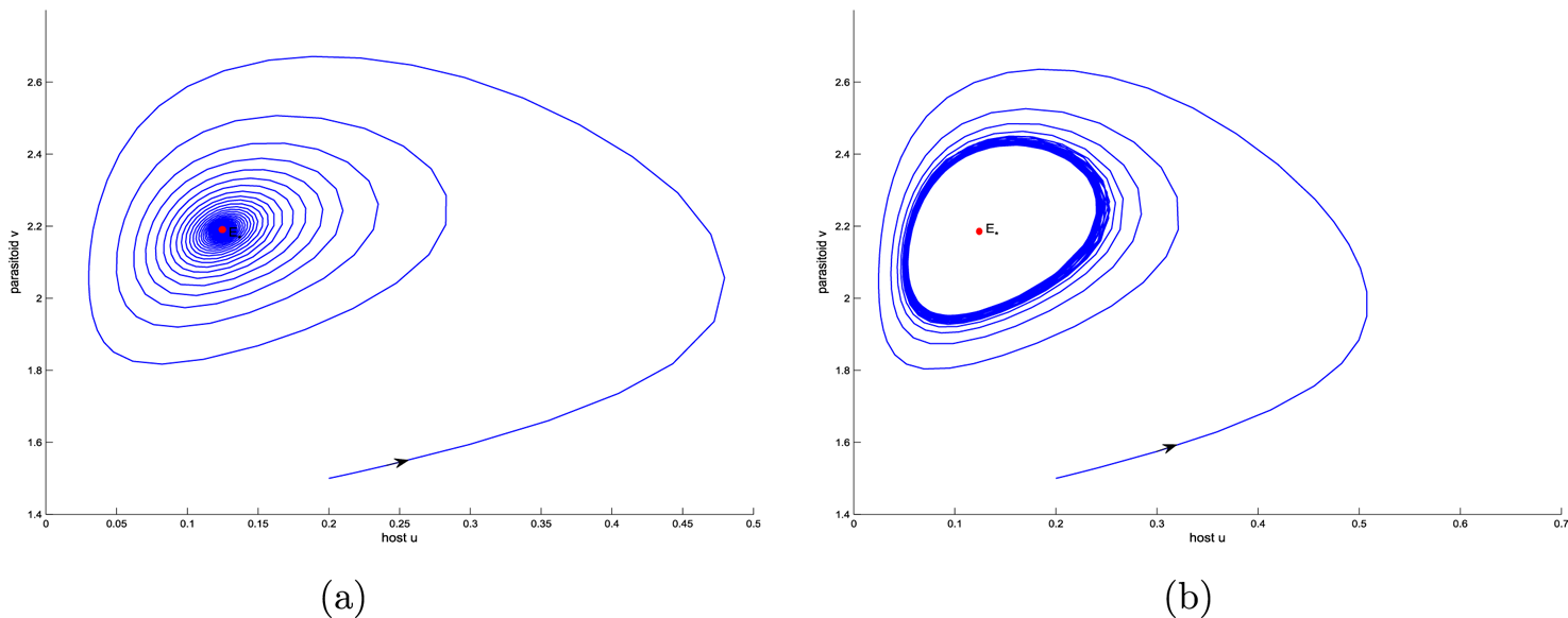
It is easy to check that $E_{*}$ is stable when $c=\frac {1}{40}>c^{H}_0=\frac {4}{175}$ (figure 1(a)), and a stable limit cycle, bifurcating from supercritical Hopf bifurcation at $E_{*}$, occurs when $c=\frac {1}{50}< c^{H}_0$ (figure 1(b)).

Figure 1.

(a) $E_{*}$ of system (2.1) is stable when $c=\frac {1}{40}>c^{H}_0=\frac {4}{175}$; (b) $E_{*}$ of system (2.1) is unstable and surrounded by a stable limit cycle when $c=\frac {1}{50}< c^{H}_0$.

3. System (1.3) with local intraspecific prey competition

In this section, we consider system (1.3) with local intraspecific prey competition, i.e. the nonlocal term $\hat {u}$ in (1.3) is reduced to $u(x,\,t)$.

3.1. Turing instability of the reaction–diffusion system

In this subsection, we consider the Turing instability of the positive constant steady state $E_{*}$ in reaction–diffusion system (1.3) when $(a,\,b,\,c,\,e)\in {U_{1}}$.

Proposition 3.1 The solutions of (1.3) are non-negative. Moreover, the non-negative solution $(u,\,v)$ of system (1.3) satisfies

\[ \mathop{\limsup}\limits_{t\rightarrow\infty}\mathop{\max}\limits_{\bar{\Omega}}u(x,t)\leq1,\quad \mathop{\limsup}\limits_{t\rightarrow\infty}\mathop{\max}\limits_{\bar{\Omega}}v(x,t)\leq1+\frac{e}{1+a}. \]

Proof. Since both the $u$-axis and $v$-axis are invariant lines, if the initial values are non-negative, then solutions of system (1.3) are also non-negative. According to comparison principle, we have

\[ u(1-u)-\frac{buv}{a+u}\leq u(1-u),\quad (x,t)\in\Omega\times[0,\infty), \]

hence, there exists a $T\in (0,\,\infty )$ such that $u(x,\,t)\leq 1+\epsilon$ in $\bar {\Omega }\times [T,\,\infty )$ for any $\epsilon >0$. Moreover,

\[ cv\left(1+\frac{eu}{a+u}-v\right)\leq cv\left(1+\frac{e(1+\epsilon)}{a+1+\epsilon}-v\right),\quad x\in\bar{\Omega},\quad t\in[T,\infty), \]

then again by comparison principle, we have

\[ \mathop{\limsup}\limits_{t\rightarrow\infty}\mathop{\max}\limits_{\bar{\Omega}}v(x,t)\leq1+\frac{e+\epsilon}{1+a+\epsilon}, \]

by the arbitrariness of $\epsilon$, the conclusion holds.

The linear part of system (1.3) is

(3.1)\begin{equation} \begin{array}{@{}ll@{\vskip-6pt}} \left(\begin{array}{@{}cc@{}} \displaystyle\dfrac{\partial{u}}{\partial{t}}\\ \displaystyle\dfrac{\partial{u}}{\partial{t}} \end{array}\!\!\!\right)=L\left(\begin{array}{@{}cc@{}} u\\ v\end{array}\!\!\!\right)=D\left(\begin{array}{@{}cc@{}}u_{xx}\\v_{xx}\end{array}\!\!\!\right)+J\left(\begin{array}{@{}cc@{}} u\\ v\end{array}\!\!\!\right)\end{array} \end{equation}

where

\[ {D}={\left(\begin{array}{@{}cc@{}} d_{1} & 0\\ 0 & d_{2}\end{array}\right),} \]

and $J=J_{0}$. $L$ is a linear operator with domain $D_{L}=X_{C}:=X\oplus {\rm i}X=\{x_{1}+{\rm i}x_{2}:x_{1},\,x_{2}\in X\}$ and

\begin{align*} X& :=\{(u,v)\in H^{2}[(0,l\pi)]\times H^{2}[(0,l\pi)]\big{|}u_{x}(0,t)=u_{x}(l\pi,t)\\& =v_{x}(0,t)=v_{x}(l\pi,t)=0\}, \end{align*}

where $H^{2}[(0,\,l\pi )]$ represent a standard Sobolev space.

Define ($k\in \mathbb {N}$):

\[ {J_{k}}={\left(\begin{array}{@{}cc@{}} s_{1}-u_*-d_{1}\left(\dfrac{k}{l}\right)^{2} & -\delta_{1}\\ c\delta_{2} & -cv_{*}-d_{2}\left(\dfrac{k}{l}\right)^{2}\end{array}\right),} \]

then the corresponding characteristic equation of $J_{k}$ is

(3.2)\begin{equation} \mathcal{P}_{k}(\lambda)={\lambda}^{2}-\mathcal{T}_{k}\lambda+\mathcal{M}_{k}, \end{equation}

in which

\begin{align*} \mathcal{T}_{k}& =\mathcal{T}_{0}-(d_{1}+d_{2})\left(\frac{k}{l}\right)^{2},\\ \mathcal{M}_{k}& =d_{1}d_{2}\left(\frac{k}{l}\right)^{4} +(cv_{*}d_{1}-(s_{1}-u_*)d_{2})\left(\frac{k}{l}\right)^{2}+\mathcal{M}_{0}. \end{align*}

Obviously, $B_{i}$ ($i=1,\,2,\,3$) and $E_{*}$ are all constant steady states. When $(a,\,b,\,c,\,e)\in {U_{1}}$, $B_{i}$ ($i=1,\,2,\,3$) are still unstable, and $E_{*}(u_{*},\,v_{*})$ is locally asymptotically stable for system (1.3) if and only if one of the following conditions holds:

(i) $u_{*}\geq {(1-a)}/{2}$;
(ii) $u_{*}<{(1-a)}/{2}$, $c>c^{H}_0$, $cv_{*}d_{1}-(s_{1}-u_*)d_{2}\geq 0$.

Next, we study the instability and stability of the positive constant steady state $E_{*}$ induced by diffusion.

Because $\mathcal {T}_k<0$ and $\mathcal {M}_{k}>0$ for any $k\geq 0$ when $u_{*}\geq {(1-a)}/{2}$ and $(a,\,b,\,c,\,e)\in {U}_{1}$, we consider Turing instability under the following conditions:

(3.3)\begin{equation} c>c^{H}_0,\quad u_{*}<\frac{1-a}{2},\quad (a,b,c,e)\in{U}_{1}, \end{equation}

where $U_{1}$ and $c^{H}_0$ are given in (2.3) and (2.7), respectively. Note that $\mathcal {T}_{k}<0$ for any positive integer $k$ if $u_{*}<{(1-a)}/{2}$ and $c>c^{H}_0$, thus to make sure Turing instability occurs, we need find the parameter conditions for $\mathcal {M}_{k}<0$. Define:

(3.4)\begin{equation} U_{2}=\left\{(a,b,c,e,u_{*})|u_{*}<\frac{1-a}{2},\ 1>a\geq\frac{1}{2}, \ a>b>0, \ c>0, \ e>0\right\}. \end{equation}

Next, we discuss diffusion-induced instability at $E_{*}$ for system (1.3).

We define

(3.5)\begin{equation} \mathcal{B}=(s_{1}-u_*)d_{2}-cv_{*}d_{1}. \end{equation}

To ensure that Turing instability occurs, we need to find appropriate parameter conditions such that $\mathcal {M}_{k}<0$ for some $k\in \mathbb {N}$. Hence, we let:

\[ \mathcal{B}>0\quad {\rm and}\quad (\mathcal{M}_{k})_{\min}=\mathcal{M}_{l\sqrt{{\mathcal{B}}/{2d_{1}d_{2}}}}=\mathcal{M}_{0}-\frac{{\mathcal{B}}^{2}}{4d_{1}d_{2}}<0, \]

which are equivalent to

\[ \mathcal{B}>2\sqrt{d_{1}d_{2}\mathcal{M}_{0}}, \]

then we have the following results.

Lemma 3.2 Suppose $(a,\,b,\,c,\,e,\,u_{*})\in {U}_{2}$, $c>c^{H}_0$ and $\mathcal {B}>2\sqrt {d_{1}d_{2}\mathcal {M}_{0}}$, then diffusion-induced Turing instability occurs for system (1.3).

Example 3.3 Choosing $(a,\,b,\,c,\,e,\,d_{1},\,d_{2})=(\frac {1}{2},\,\frac {1}{3},\,\frac {1}{25},\,\frac {203}{48},\,\frac {1}{18},\,3)$, we can get $(u_{*},\,v_{*})=(\frac {1}{12},\,\frac {77}{48})$, and

(i) if $l=1$, then for any positive integer $k$, we have $\mathcal {M}_{k}>0$. Hence, $E_{*}$ is a stable constant steady state with respect to systems (1.3) (see figure 2(a));
(ii) if $l=3$, then there exists a unique positive integer $k=2$, such that $\mathcal {M}_{2}=-\frac {5921}{453\,600}<0$. Hence, $E_{*}$ is an unstable equilibrium with respect to system (1.3) (see figure 2(b)).

Figure 2.

Turing instability of the spatially homogeneous steady state $E_*(u_*,\,v_*)$: (a) $l=1$, $E_{*}$ is stable with respect to systems (1.3); (b) $l=3$, $E_{*}$ is unstable with respect to system (1.3). $u_{0}(x)=\frac {1}{12}-0.001\cos (x),\, v_{0}(x)=\frac {77}{48}+0.001\cos (x)$.

3.2. Bifurcations of the reaction–diffusion system

In this subsection, we discuss the Hopf bifurcation and Turing–Hopf bifurcation for system (1.3) around $E_{*}$ under the parameter condition $U_{2}$, where $U_{2}$ is given in (3.4).

3.2.1. Hopf bifurcation.

In theorem 2.2 we discussed the existence of temporal periodic solutions for system (1.3) when all the diffusion coefficients are equal to zero. Now, we want to explore the Hopf bifurcation when the diffusion coefficients are not all zero and $(a,\,b,\,c,\,e,\,u_{*})\in {U_{2}}$, where $U_{2}$ is given in (3.4).

Here, we still use $c$ as the bifurcation parameter, the necessary conditions for a Hopf bifurcation at $c=c^{H}_{i}$ ($i=0,\,1,\,2,\ldots$) are

(3.6)\begin{align} & \mathcal{T}_{i}|_{c=c^{H}_{i}}=0,\quad \mathcal{M}_{i}|_{c=c^{H}_{i}}>0, \end{align}

(3.7)\begin{align} & \mathcal{T}_{j}|_{c=c^{H}_{i}}\neq0,\quad \mathcal{M}_{j}|_{c=c^{H}_{i}}\neq0,\quad j\neq i, \end{align}

where $\mathcal {T}_{k}$ and $\mathcal {M}_{k}$ are given in (3.2).

Next, we first explore the existence and bifurcating direction of spatially homogeneous periodic orbits for system (1.3), i.e. $i=0$, $c=c^{H}_0$ in (3.6) and (3.7). Obviously, $\mathcal {T}_{0}=0$ and $\mathcal {M}_{0}>0$ hold for $c=c^{H}_0$ and $(a,\,b,\,c,\,e,\,u_{*})\in {U_{2}}$. Moreover, at $c=c^{H}_0$, $\mathcal {T}_{k}<0$ for any positive integer $k$. According to the expression of $\mathcal {M}_{k}$, we let:

(3.8)\begin{equation} 2\sqrt{d_1d_2\mathcal{M}_{0}}>\mathcal{B}, \end{equation}

which implies that

(3.9)\begin{equation} (\mathcal{M}_{k})_{\min}>0 \end{equation}

for any positive integer $k$. Under these conditions, we have a single pair of complex eigenvalues with zero real part given by $\lambda =\pm \beta _{0}{\rm i}$ (where $\beta _{0}=\sqrt {\mathcal {M}_{0}}$) and

(3.10)\begin{equation} \frac{{\rm d} {\rm Re}(\lambda(c))}{{\rm d}c}\bigg | _{c=c^{H}}={-}\frac{v_{*}}{2}\neq0. \end{equation}

To get the stability of the bifurcated periodic solutions we need to know the behaviour of system (1.3) in its centre manifold at the bifurcation point. First, we define a conjugate operator of $L$ which was defined in (3.1) as follows:

(3.11)\begin{equation} \begin{array}{@{}ll@{}} L^{*}{\left(\begin{array}{@{}cc@{}} u\\ v\end{array}\!\!\!\right)}=D{\left(\begin{array}{@{}cc@{}}u_{xx}\\ v_{xx}\end{array}\!\!\!\right)}+J^{*}{\left(\begin{array}{@{}cc@{}} u\\ v\end{array}\!\!\!\right)}. \end{array} \end{equation}

Here, $J^{*}=J^{T}(E_{*})$ and $L^{*}$ are also defined in domain $X\!$.

Let:

\[ q={\left(\begin{array}{@{}cc@{}}q_{1}\\q_{2}\end{array}\!\!\!\right)}={\left(\begin{array}{@{}cc@{}}1\\ \displaystyle\dfrac{s_{1}-u_*}{\delta_{1}}-\dfrac{\beta_{0}}{\delta_{1}}{\rm i}\end{array}\!\!\!\right)},\quad q^{*}={\left(\begin{array}{@{}cc@{}} q^{*}_1\\ q^{*}_{2}\end{array}\!\!\!\right)}=\frac{1}{2l\beta_{0}\pi}{\left(\begin{array}{@{}cc@{}} \beta_{0}+(s_1-u_*){\rm i} \\ - \delta_{1}{\rm i}\end{array}\!\!\!\right),} \]

where $\beta _{0}=\beta (c^{H})$ and $\langle m,\,n\rangle =\int _{0}^{l\pi }\overline {m}^{T}n\,{\rm d}x$ for any $m\in D_{L^{*}}$ and $n\in D_{L}$, which denotes the inner product in $L^{2}[(0,\,\pi )]\times L^{2}[(0,\,\pi )]$. It is easy to check that $\langle L^{*}m,\,n\rangle =\langle m,\,Ln\rangle$, $Lq={\rm i}\beta _{0}q$, $L^{*}q^{*}=-{\rm i}\beta _{0}q^{*}$, $\langle q^{*},\,q\rangle =1$ and $\langle q^{*},\,\bar {q}\rangle =0$.

Following the calculating procedure in Hassard et al. [Reference Hassard, Kazarinoff and Wan18] (see also [Reference Yi, Wei and Shi42]), we obtain:

\[ {\rm Re}(\sigma_{1}(c^{H}_0))=4\frac{u_{*}(1-a-2u_{*})}{8(a+u_{*})^{6}(1-u_{*})\mathcal{M}_{0}}\sigma_{11}, \]

where $\sigma _{11}$ is given in (2.8). Then, we have the following results.

Theorem 3.4 If $(a,\,b,\,c,\,e,\,u_{*})\in {U_{2}}$ and $2\sqrt {d_1d_2\mathcal {M}_{0}}>\mathcal {B}$, then system (1.3) undergoes a 0-mode Hopf bifurcation around $E_{*}$ at $c=c^{H}_0\!$. Moreover,

(1) if $\sigma _{11}<0$, then the Hopf bifurcation is supercritical and the bifurcating (spatially homogeneous) periodic solutions are asymptotically stable;
(2) if $\sigma _{11}>0$, then the Hopf bifurcation is subcritical and the bifurcating (spatially homogeneous) periodic solutions are unstable.

Example 3.5 Fix $a=\frac {1}{2}$, $b=d_{2}=\frac {1}{3}$, and $e=\frac {7}{2}$, choose $d_{1}=0.015$ and $c=0.03<0.031=c^{H}_0$, then we have ${\rm Re}(\sigma _{1}(c^{H}_0))=-1.615<0$, which means that the bifurcating periodic solutions are orbitally asymptotically stable (see figure 3).

Figure 3.

Stable spatially homogeneous periodic solution bifurcating from 0-mode Hopf bifurcation in system (1.3), where $(a,\,b,\,e)=(\frac {1}{2},\,\frac {1}{3},\,\frac {7}{2})$, $l=2$, $(d_{1},\,d_{2})=(0.015,\,\frac {1}{3})$, $c=0.03< c^{H}=0.031$, $(u_{0}(x),\,v_{0}(x))=(0.1-0.01 \cos (1.5x),\,1.8-0.05\cos (1.5x))$.

Next, we consider the spatially nonhomogeneous Hopf bifurcations for system (1.3) with $k\geq 1$.

Define:

(3.12)\begin{equation} \mathcal{A}_{1}=\delta_{1}\delta_{2}-(s_{1}-u_*)v_{*},\quad \mathcal{A}_{2}=\sqrt{\delta_{1}\delta_{2}(\delta_{1}\delta_{2}-(s_{1}-u_*)v_{*})}, \end{equation}

where $\mathcal {A}_{1}>0$ since ${\rm Det}(J(E_{*}))>0$.

If $d_{1}+d_{2}\geq (s_{0}-u_*)l^{2}$, then $\mathcal {T}_k<0$ for any positive integer $k$. If $d_{1}+d_{2}< (s_{1}-u_*)l^{2}$, then there exists a largest positive integer $\check {k}$ such that $(d_{1}+d_{2})k^{2}< (s_{1}-u_*)l^{2}$ for $1\leq k\leq \check {k}$, and $(d_{1}+d_{2})k^{2}\geq (s_{1}-u_*)l^{2}$ for $k>\check {k}$. Moreover, from $\mathcal {T}_k=0$ ($1\leq k\leq \check {k}$), we have $c=c_{k}^{H}$, where

(3.13)\begin{equation} c_{k}^{H}=\frac{(s_{1}-u_*)l^{2}-(d_{1}+d_{2})k^{2}}{v_{*}l^{2}} \quad (1\leq k\leq\check{k}). \end{equation}

On the other hand, substituting $c_{k}^{H}$ into $\mathcal {M}_{k}$, we have

\[ \mathcal{M}_{k}=\left((s_{1}-u_*)-d_1\left(\frac{k}{l}\right)^2\right)\left(d_1\left(\frac{k}{l}\right)^2+\frac{\mathcal{A}_{1}}{v_*}\right)-d_2\left(\frac{k}{l}\right)^2\frac{(s_{1}-u_*)v_*+\mathcal{A}_{1}}{v_*}, \]

it is obvious that $\mathcal {M}_{k}<0$ for any positive integer $k$ if $(s_{1}-u_*)\leq d_1({1}/{l})^2$. If $(s_{1}-u_*)> d_1({1}/{l})^2$, then there exists a largest positive integer $\hat {k}$ such that $(s_{1}-u_*)> d_1({k}/{l})^2$ for $1\leq k\leq \hat {k}$, and $(s_{1}-u_*)\leq d_1({k}/{l})^2$ for $k>\hat {k}$. It is easy to see that $\check {k}\leq \hat {k}$. From $\mathcal {M}_{k}=0$, we have $d_2=d_2^{k}\triangleq ({(\mathcal {A}_{1}l^{2}+d_{1}v_{*}k^{2})((s_{1}-u_*)l^{2}-d_{1}k^{2})})/({k^{2}l^{2}(\mathcal {A}_{1}+(s_{1}-u_*)v_{*})})$, and $d_2^{k}$ is decreasing with respect to $k^2$. Let:

(3.14)\begin{equation} d_{2}^{*}=\frac{(\mathcal{A}_{1}l^{2}+d_{1}v_{*}{\hat{k}}^{2})((s_{1}-u_*)l^{2}-d_{1}{\hat{k}}^{2})}{{\hat{k}}^{2}l^{2}(\mathcal{A}_{1}+(s_{1}-u_*)v_{*})}, \end{equation}

where $c_{0}$ and $\mathcal {A}_{1}$ are given in (2.4) and (3.12), respectively. We have the following results.

Theorem 3.6 Assume $(a,\,b,\,c,\,e,\,u_{*})\in {U_{2}}$, $d_{1}+d_{2}< (s_{1}-u_*)l^{2}$ and $d_{2}< d_{2}^{*}$ hold, then system (1.3)undergoes a $k$-mode Hopf bifurcation at $c=c_{k}^{H}$ for $k\in [1,\,\check {k}]$, where the characteristic equation $\mathcal {P}_{k}(\lambda )=0$ has a pair of purely imaginary roots and other roots of $P_{k}(\lambda )=0$ with non-zero real parts.

Proof. By $(a,\,b,\,c,\,e,\,u_{*})\in {U_{2}}$, we have $(s_{1}-u_*)>0$. For fixed $k\in [1,\,\check {k}]$ and $c=c_{k}^{H}$, we have $\mathcal {T}_k=0$ and $\mathcal {M}_{k}>0$ since $d_{1}+d_{2}<(s_{1}-u_*)l^{2}$ and $d_{2}< d_{2}^{*}$. Moreover, for other integer $k\geq 0$, we have $\mathcal {T}_k\neq 0$ and $\mathcal {M}_{k}\neq 0$. These complete the proof.

Example 3.7 Fixed $a=\frac {1}{2}$, $b=\frac {1}{4}$, and $e=\frac {95}{16}$, if we chose $d_{1}=\frac {1}{4}$, $d_{2}=\frac {1}{28}$, and $l=8$, then $\hat {k}=\check {k}=3$ and $d^{*}_{2}=\frac {4807}{46\,080}>\frac {1}{28}$. Hence, according to theorem 3.6, system (1.3) exhibits a $k$-mode Hopf bifurcation for $k=1,\,2,\,3$, which are spatially nonhomogeneous.

3.2.2. Turing–Hopf bifurcation.

In this subsection, we consider the existence of Turing–Hopf bifurcations around $E_{*}$ in system (1.3) under the condition $U_{2}$, where $U_{2}$ is given in (3.4).

According to Jiang et al. [Reference Jiang, An and Shi19], if there exists a positive integer $k_{1}$ and a non-negative integer $k_{2}$ ($k_{2}\neq {k}_{1}$) such that $\mathcal {P}_{k_{1}}(\lambda )=0$ has a simple zero root and $\mathcal {P}_{k_{2}}(\lambda )=0$ has a pair of purely imaginary roots, while all other eigenvalues of $\mathcal {P}_{k}(\lambda )=0$ have non-zero real parts, and the corresponding transversal conditions hold, then we say that a $(k_{1},\,k_{2})$-mode Turing–Hopf bifurcation occurs.

Let $\mathcal {P}_{k}(0)=0$ ($k\in \mathbb {N}$), then we have

\[ d_{1}d_{2}\left(\frac{k}{l}\right)^{4}+(cv_{*}d_{1}-(s_{1}-u_*)d_{2})\left(\frac{k}{l}\right)^{2}+c(\delta_{1}\delta_{2}-(s_{1}-u_*)v_{*})=0, \]

from which we have

(3.15)\begin{equation} c=c_{k}(d_{1})\triangleq\frac{{d}_{2}k^{2}((s_{1}-u_*)l^{2}-d_{1}k^{2})}{v_{*}d_{1}k^{2}l^{2}+\mathcal{A}_{1}l^{4}},\quad d_{1}\in\bigg(0,\frac{l^{2}}{k^{2}}(s_{1}-u_*)\bigg), \end{equation}

where $\mathcal {A}_{1}$ is defined in (3.12). Thus, system (1.3) may undergo $k$-mode Turing bifurcation if $c=c_{k}(d_{1})$, $d_{1}\in (0,\,{((s_{1}-u_*)l^{2})}/{k^{2}})$ and $k\in \mathbb {N}$.

Theorem 3.8 Assume $(a,\,b,\,c,\,e,\,u_{*})\in {U_{2}}$, if $k\geq k_{*}=\left \lfloor {l}\sqrt {{\mathcal {A}_{1}}/{d_{2}v_{*}}}\right \rfloor +1$, then system (1.3) undergoes a $(k,\,0)$-mode Turing–Hopf bifurcation at $E_{*}$ for $(d_{1},\,c)=(d_{1}^{k},\,c^{H}_0)$. Moreover, when $(d_{1},\,c)=(d_{1}^{k^{*}_{0}},\,c^{H}_0)$, system (1.3) undergoes a $(k^{*}_{0},\,0)$-mode Turing–Hopf bifurcation, where all other eigenvalues of $\mathcal {P}_{k}(\lambda )=0$ have negative real parts except a simple zero eigenvalue and a pair of pure imaginary eigenvalues.

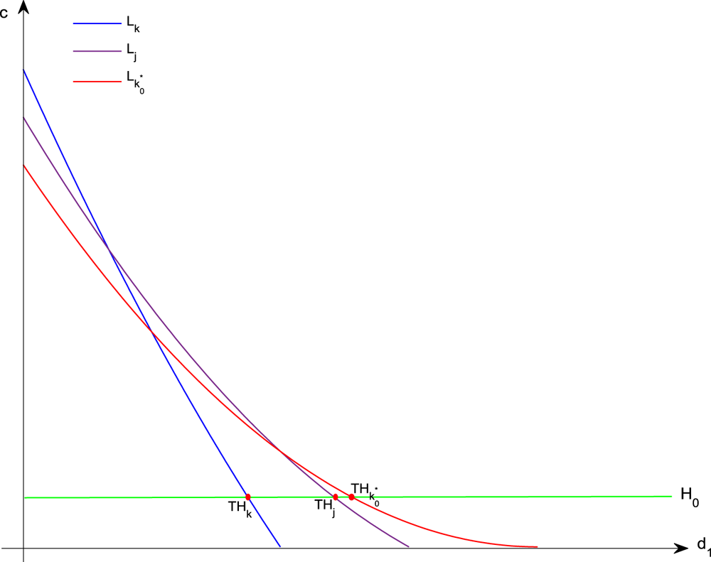
Proof. First, we denote the curves $c=c_{k}(d_{1})$ in the $(d_{1},\,c)$-plane by $L_{k}$, i.e.:

\[ L_{k}:c=c_{k}(d_{1}),\quad 0< d_{1}<\frac{(s_{1}-u_*)l^{2}}{k^{2}},\quad k\in\mathbb{N}, \]

and denote the 0-mode Hopf bifurcation curve in the $(d_{1},\,c)$-plane by $H_0$, i.e.:

\[ H_{0}:c=c^{H}_0, \]

where $c^{H}_0$ is defined in (2.6).

Second, we explore the existence of Turing–Hopf bifurcation point. From (3.15) we have ${{\rm d}c_{k}(d_{1})}/{{\rm d}d_{1}}=-({{\rm d}_{2}\delta _{1}\delta _{2}k^{4}}/({(v_{*}d_{1}k^{2}+\mathcal {A}_{1}l^2)^{2}}))<0$, which implies that $c_{k}(d_{1})$ is monotonically decreases in $d_{1}$. By straightforward calculation we have $\lim \nolimits _{d_{1}\rightarrow 0^+}c_{k}(d_{1})=({(s_{1}-u_*)d_{2}k^{2}})/{\mathcal {A}_{1}l^{2}}>{(s_{1}-u_*)}/{v_{*}}=c^{H}_0$ if $k\geq k_{*}\triangleq \left \lfloor l\sqrt {{\mathcal {A}_{1}}/{d_{2}v_{*}}}\right \rfloor +1$ ($\lfloor \cdot \rfloor$ denotes the floor function). Combining the above results with $\lim \nolimits _{d_{1}\rightarrow {((s_{1}-u_*)l^{2})}/{k^{2}}}c_{k}(d_{1})=0$, we know that there exists a unique $d_{1}= d_{1}^{k}\in (0,\,{(l^2(s_{1}-u_*))}/{k^{2}})$ such that $c_{k}(d^{k}_{1})=c^{H}_0$ for $k\geq k_{*}$ (see figure 4). Thus, the Turing–Hopf bifurcation point ${TH}_k( d_{1}^{k},\,c^{H}_0)$ exists for $k\geq k_{*}$, where

(3.16)\begin{equation} d_{1}^{k}=\frac{(s_{1}-u_*)(v_{*}d_{2}k^{2}-\mathcal{A}_{1}l^{2})l^{2}}{v_{*}k^{2}((s_{1}-u_*)l^{2}+d_{2}k^{2})}, \quad k\geq{k_{*}}. \end{equation}

Moreover, we have

\[ \frac{{\rm d}d_{1}^{k}}{{\rm d}k^{2}}= \frac{(s_{1}-u_*)l^{2}({-}v_{*}d^{2}_{2}k^{4}+2d_{2}\mathcal{A}_{1}l^{2}k^{2}+(s_{1}-u_*)\mathcal{A}_{1}l^{4})}{v_*k^{4}((s_{1}-u_*)l^{2}+d_{2}k^{2})^{2}}. \]

Next, we discuss the sign of ${{\rm d}d_{1}^{k}}/{{\rm d}k^{2}}$. It is obviously that ${{\rm d}d_{1}^{k}}/{{\rm d}k^{2}}$ has the same sign with $\varphi (k^{2})\triangleq -v_{*}d^{2}_{2}k^{4}+2d_{2}\mathcal {A}_{1}l^{2}k^{2}+(s_{1}-u_*)\mathcal {A}_{1}l^{4}$. Let $w=k^{2}$, then $\varphi (w)=-v_{*}d_{2}^{2}w^{2}+2d_{2}\mathcal {A}_{1}l^{2}w+(s_{1}-u_*)\mathcal {A}_{1}l^{4}$. Since $\lim \nolimits _{w\rightarrow 0^+}\varphi (w)=(s_{1}-u_*)\mathcal {A}_{1}l^{4}>0$, and $\lim \nolimits _{w\rightarrow \infty }\varphi (w)=-\infty$, there exists a unique positive $w_{*}$ satisfying $\varphi (w_{*})=0$, and $\varphi (w)>0$ in the interval $[0,\,w_{*})$. Denote:

\[ k_{m}^{0}\triangleq\lfloor \sqrt{w_{*}} \rfloor=\left\lfloor l\sqrt{\frac{\mathcal{A}_{2}+\mathcal{A}_{1}}{v_{*}d_{2}}}\right\rfloor, \]

where $\mathcal {A}_{2}$ is defined in (3.12). Define $k_{m}\triangleq \max \{k_{*},\,k_{m}^{0}\}$, then $d_{1}^{k}$ monotonically increases in the interval $[k_{*},\,k_{m}]$ for $k_{m}\geq k_{*}$, and monotonically decreases in the interval $[k_{m}+1,\,\infty )$ in $k$.

Figure 4.

Turing bifurcation curves $L_k,\, L_j,\, L_{k^{*}_{0}}$, Hopf bifurcation curve $H_0$ and Turing–Hopf bifurcation points $TH_k,\, TH_j,\, TH_{k^{*}_{0}}$ in the $(d_{1},\,c)$-plane.

We denote:

\[ k_{0}^{*}=\begin{cases} k_{m},\ \text{if}\ d_{1}^{k_{m}}>d_{1}^{k_{m}+1},\\ k_{m}+1, \ \text{if}\ d_{1}^{k_{m}}< d_{1}^{k_{m}+1},\end{cases} \]

then for any given $c=c^H_0$, $d^{k^{*}_{0}}_{1}=\max \nolimits _{k\in \mathbb {N}}\{d_{1}^{k}\}$, which is the abscissa of Turing–Hopf bifurcation point ${TH}_{k^{*}_{0}}( d^{k^{*}_{0}}_{1},\, c^{H}_0)$ (see figure 4). Thus, system (1.3) may undergo a $(k^{*}_{0},\,0)$-mode Turing–Hopf bifurcation, where all other eigenvalues of $\mathcal {P}_{k}(\lambda )=0$ have negative real parts except a simple zero eigenvalue and a pair of pure imaginary eigenvalues. If $d^{k_{m}}_{1}=d^{k_{m}+1}_{1}$, then diffusive system (1.3) may undergo Turing–Turing–Hopf bifurcation, which is a codimension-3 bifurcation, we leave it for future consideration.

When $(d_1,\,c)=(d^{k^{*}_{0}}_{1},\,c^{H}_0)$, we have $\mathcal {T}_{0}=0$, $\mathcal {M}_{0}>0$, $\mathcal {T}_{k^{*}_{0}}<0$, and $\mathcal {M}_{k^{*}_{0}}=0$. In addition, we have $\mathcal {T}_{k}<0$ for any positive integer $k$, and $\mathcal {M}_{k}>0$ for any $k\neq {k^{*}_{0}}$ since $d^{k^{*}_{0}}_{1}=\max \nolimits _{k\in \mathbb {N}}\{d_{1}^{k}\}$. This implies that the real parts of the eigenvalues of $\mathcal {P}_{k}(\lambda )=0$ ($k\neq 0,\,\;k^{*}_{0}$) are all negative. Moreover, suppose $\lambda _{1}=\alpha _{1}+{\rm i}\beta _{1}$ and $\lambda _{2}=\alpha _{2}+{\rm i}\beta _{2}$, where $\beta _{1}=\sqrt {\mathcal {M}_{0}}$ and $\alpha _{1}=\alpha _{2}=\beta _{2}=0$ when $(d_{1},\,c)=(d_{1}^{k^{*}_{0}},\,c^{H}_0)$, then we have the transversality conditions:

(3.17)\begin{align} \frac{{\rm d}\alpha_{1}}{{\rm d}c}\bigg |_{c=c^{H}_0}={-}\frac{v_{*}}{2}<0, \quad \frac{{\rm d}\alpha_{2}}{{\rm d}d_{1}}\bigg |_{d_{1}=d^{k^{*}_{0}}_{1}}=\frac{(d_{2}\left({k}/{l}\right)^{2}+(s_{1}-u_*))\left({k}/{l}\right)^{2}}{T_{k^{*}_{0}}}<0,\quad c=c^{H}_0. \end{align}

The proof is completed.

3.3. Spatiotemporal patterns via Turing–Hopf bifurcation

In this section, we calculate the normal forms of the $(k^{*}_{0},\,0)$-mode Turing–Hopf bifurcation for reaction–diffusion system (1.3) at $E_{*}$. We choose $d_{1}$ and $c$ as bifurcation parameters, let $d_{1}=d_{1}^{k^{*}_{0}}+\mu _{1},\,\;c=c^{H}_0+\mu _{2}$, and obtain the unfolding system from system (1.3) as follows:

(3.18)\begin{equation} \begin{cases} \displaystyle\frac{\partial{u}}{\partial{t}}-(d_{1}^{k^{*}_{0}}+\mu_{1})\Delta u=u\bigg(1-u-\frac{bv}{a+u}\bigg),\ x\in(0,l\pi),\ t>0,\\ \displaystyle\frac{\partial{v}}{\partial{t}}-d_{2}\Delta v=(c^{H}_0+\mu_{2})v\bigg(1-v+\frac{eu}{a+u}\bigg),\ x\in(0,l\pi),\ t>0. \end{cases} \end{equation}

The constant steady state of system (3.18) is $E_{*}$, where $u_{*}$ satisfies $f(u_{*})=0$ and $v_{*}={((1-u_{*})(a+u_{*}))}/{b}$. To apply the generic formulas developed by Jiang et al. [Reference Jiang, An and Shi19], we consider the transformation $\breve {u}=u-u_{*},\,\breve {v}=v-v_{*}$ and drop the breves, then system (3.18) is transformed into:

(3.19)\begin{equation} \begin{cases} \displaystyle\frac{\partial{u}}{\partial{t}}-(d_{1}^{k^{*}_{0}}+\mu_{1})\Delta u=(u+u_{*})\left(1-(u+u_{*})-\frac{b(v+v_{*})}{a+(u+u_{*})}\right),\\ \displaystyle\frac{\partial{v}}{\partial{t}}-d_{2}\Delta v=(c^{H}_0+\mu_{2})(v+v_{*})\left(1-(v+v_{*})+\frac{e(u+u_{*})}{a+(u+u_{*})}\right). \end{cases} \end{equation}

According to [Reference Jiang, An and Shi19], by a series of calculations, the normal form of system (1.3) restricted on the centre manifold up to third order at the Turing–Hopf singularity is

(3.20)\begin{equation} \begin{cases} \dot{z}_{1}=a_{1}(\mu)z_{1}+a_{200}z_{1}^{2}+a_{011}z_{2}\bar{z}_{2}+a_{300}z_{1}^{3}+a_{111}z_{1}z_{2}\bar{z}_{2}+h.o.t.,\\ \dot{z}_{2}={\rm i}\omega_{0}z_{2}+b_{2}(\mu)z_{2}+b_{110}z_{1}z_{2}+b_{210}z_{1}^{2}z_{2}+b_{021}z^{2}_{2}z\bar{z}_{2}+h.o.t.,\\ \dot{\bar{z}}_{2}={-}{\rm i}\omega_{0}\bar{z}_{2}+\bar{b}_{2}(\mu)\bar{z}_{2}+\bar{b}_{110}z_{1}\bar{z}_{2}+\bar{b}_{210}z_{1}^{2}\bar{z}_{2} +\bar{b}_{021}z_{2}\bar{z}_{2}^{2}+h.o.t.,\\ \end{cases} \end{equation}

where the coefficients can be directly calculated according to [Reference Jiang, An and Shi19]; here, we omit the expressions for brevity. Instead, we derive concrete expressions for normal form (3.20) by fixing parameters. Then, we present bifurcation diagrams of the Turing–Hopf bifurcation and the corresponding phase portraits to exhibit spatiotemporal dynamics for diffusive system (1.3) near the Turing–Hopf singularity.

3.3.1. $(3,\,0)$-mode Turing–Hopf bifurcation.

In this subsection, we set $(a,\,b,\,e, d_{2},\,l)=(\frac {1}{2},\,\frac {1}{3},\,\frac {7}{2},\,\frac {1}{3},\,2)$. By straightforward calculations for system (1.3), we have $s_{1}-u_*=0.0505$, $\mathcal {M}_{0}=0.01169$, $(u_{*},\,v_{*})=(0.109,\,1.629)$, $k^{*}_{0}=3$, and $d^{k^{*}_{0}}_{1}=0.014534$. Then, we have $k_{1}=3$ and $k_{2}=0$. The Turing bifurcation curve is

\begin{align*} L_{3}:c& =c_{3}(d_{1})=\frac{{\rm d}_{2}k^{2}(l^{2}c_{0}-d_{1}k^{2})}{v_{*}d_{1}l^{2}k^{2}+(\delta_{1}\delta_{2}-c_{0}v_{*})l^{4}}\\ & =\frac{0.0103-0.4604d_{1}}{d_{1}+0.1028},\quad 0< d_{1}<0.0224, \end{align*}

Hopf bifurcation curve is $c=c^{H}_0=0.031$, and $(3,\,0)$-mode Turing–Hopf bifurcation point is $(d_1,\, c)=(0.014534,\, 0.031)$.

Furthermore, for the above given parameters, the normal form system (3.20) truncated to order 3 for the $(3,\,0)$-mode Turing–Hopf bifurcation is

(3.21)\begin{align} \dot{z}_{1}& ={-}(2.3011\mu_{1}+0.5495\mu_{2})z_{1}-3.2542z_{1}^{3}-5.9346z_{1}z_{2}\bar{z}_{2},\nonumber\\ \dot{z}_{2}& =0.1081iz_{2}+(1.7432i-0.8141)\mu_{2}z_{2}+(0.01822i-2.1171)z_{1}^{2}z_{2}\nonumber\\ & \quad -(1.6147+1.2983i)z_{2}^{2}\bar{z}_{2},\nonumber\\ \dot{\bar{z}}_{2}& ={-}0.1081i\bar{z}_{2}-(1.7432i+0.8141)\mu_{2}\bar{z}_{2}-(0.01822i+2.1171)z_{1}^{2}\bar{z}_{2}\nonumber\\ & \quad-(1.6147-1.2983i)z_{2}\bar{z}^{2}_{2}. \end{align}

Let $z_{1}=r$, $z_{2}=\rho \cos \theta +{\rm i}\rho \sin \theta$, $\bar {z}_{2}=\rho \cos \theta -{\rm i}\rho \sin \theta$, and drop the equation of $\theta$, then system (3.21) becomes

(3.22)\begin{align} \dot{r}& ={-}(2.3011\mu_{1}+0.5495\mu_{2})r-3.2542r^3-5.9346r\rho^{2},\nonumber\\ \dot{\rho}& ={-}0.8141\mu_{2}\rho-2.1171r^{2}\rho-1.6147\rho^{3}. \end{align}

The equilibria for system (3.22) are

\begin{align*} E_{0}& =(0,0),\\ E^{{\pm}}_{1}& =({\pm}\sqrt{-(0.7071\mu_{1}+0.1689\mu_{2})},0),\;\;{\rm for}\;\;0.7071\mu_{1}+0.1689\mu_{2}<0,\\ E_{2}& =(0,\sqrt{-0.5042\mu_{2}}),\;\;{\rm for}\;\;\mu_{2}<0,\\ E^{{\pm}}_{3}& =({\pm}\sqrt{0.5083\mu_{1}-0.5396\mu_{2}},\sqrt{-0.6665\mu_{1}+0.2033\mu_{2}}),\;\;{\rm for}\;\;0.5083\mu_{1}\\ & \quad-0.5396\mu_{2}>0,\quad -0.6665\mu_{1}+0.2033\mu_{2}>0. \end{align*}

The critical bifurcation curves for system (3.22) are

(3.23)\begin{align} H_{0}:\;\mu_{2}& =0; \quad T:\;\mu_{2}={-}4.1876\mu_{1};\nonumber \\ \quad T_{1}:\;\mu_{2}& =0.9421\mu_{1},\;\;\mu_{1}\leq0; \quad T_{2}:\;\mu_{2}=3.2786\mu_{1},\;\;\mu_{1}\leq0, \end{align}

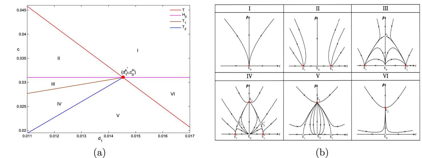
the dynamics and bifurcations for system (3.22) are similar to Case Ib in section 7.5 of [Reference Guckenheimer and Holmes16]. Therefore, the bifurcation curves in the $(d_{1},\,c)$-plane, still denoted by $H_{0}$, $T$, $T_{1}$, and $T_{2}$, respectively, are shown in figure 5(a), where

(3.24)\begin{align} & H_{0}:\,c=c^{H}_0,\quad T:\;c=c^{H}_0-4.1876(d_{1}-d^{k^{*}_{0}}_{1}),\nonumber\\ & T_{1}:\,c=c^{H}_0+0.9421(d_{1}-d^{k^{*}_{0}}_{1}),\quad d_{1}\leq d^{k^{*}_{0}}_{1},\nonumber\\ & T_{2}:\;c=c^{H}_0+3.2786(d_{1}-d^{k^{*}_{0}}_{1}),\quad d_{1}\leq d^{k^{*}_{0}}_{1}. \end{align}

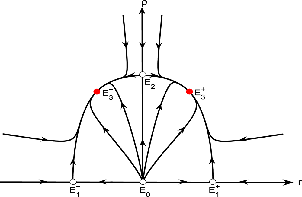
The small neighbourhood around the point $(d^{k_{0}^{*}}_{1},\,c^{H}_0)$ in the $(d_{1},\,c)$-plane is divided into six regions by these bifurcation curves. In each region, the dynamics of system (3.22) can be described by the corresponding phase portraits in figure 5(b).

Figure 5.

$(3,\,0)$-mode Turing–Hopf bifurcation diagram in the $(d_{1},\,c)$-plane for system (1.3) and the corresponding phase portraits for system (3.22).

The equilibria $E_{0}$, $E_{1}$, $E^{\pm }_{2}$, and $E^{\pm }_{3}$ of normal form system (3.22) corresponding to the positive constant steady state, the spatially homogeneous periodic solution, the positive non-constant steady states, and spatially nonhomogeneous periodic solutions of system (1.3) (or (3.18)), respectively. Thus, the dynamics of system (1.3) (or (3.18)) near the Turing–Hopf bifurcation singularity in the $(d_{1},\,c)$-plane can be classified as follows:

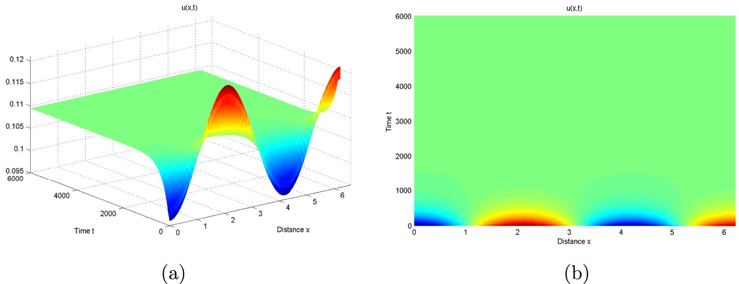
(1) When $(d_{1},\,c)=(0.0155,\,0.032)\in {\rm I}$, system (3.18) exhibit monostability: a spatially homogeneous steady state, which is asymptotically stable in region I and unstable in other regions (see figure 6).
(2) When $(d_{1},\,c)=(0.0135,\,0.032)\in {\rm II}$, system (1.3) exhibits bistability: a pair of spatially nonhomogeneous steady states. For different initial values, system (3.18) converges to one of these two spatially nonhomogeneous steady states (see figure 7).
(3) When $(d_{1},\,c)=(0.01,\,0.03)\in {\rm III}$, an unstable spatially homogeneous periodic solution occurs, and system (3.18) still exhibits bistability: a pair of spatially nonhomogeneous steady states. Moreover, system (3.18) evolves from the transient spatially homogeneous periodic solution to one of spatially nonhomogeneous steady states (see figure 8).
(4) When $(d_{1},\,c)=(0.0135,\,0.029)\in {\rm IV}$, a pair of unstable spatially nonhomogeneous periodic solutions occur, and system (3.18) exhibits tristability: two spatially nonhomogeneous steady states and a spatially homogeneous periodic solution. For different initial values, system (3.18) evolves from the spatially homogeneous steady state to a transient spatially nonhomogeneous periodic solution, and finally to the stable spatially homogeneous periodic solution (see figure 9(a) and (b)), or finally tends to one of spatially nonhomogeneous steady states (see figure 9(c)–(f)).
(5) When $(d_{1},\,c)=(0.014,\,0.025)\in {\rm V}$, a pair of unstable spatially nonhomogeneous periodic solutions disappear and system (3.18) exhibits monostability: a spatially homogeneous periodic solution (see figure 10).
(6) When $(d_{1},\,c)=(0.0155,\,0.028)\in {\rm VI}$, a pair of unstable spatially nonhomogeneous steady states disappear and system (3.18) exhibits monostability: a spatially homogeneous periodic solution (see figure 11).

Figure 6.

When $(d_{1},\,c)\in {\rm I}$ in figure 5(a) for the $(3,\,0)$-mode Turing–Hopf bifurcation, system (3.18) exhibits monostability: a positive constant steady state $E_{*}(0.109,\,1.629)$.

Figure 7.

When $(d_{1},\,c)\in {\rm II}$ in figure 5(a) for the $(3,\,0)$-mode Turing–Hopf bifurcation, system (3.18) exhibits bistability: (a),(b) One spatially nonhomogeneous steady state and (c,d): the other spatially nonhomogeneous steady state.

Figure 8.

When $(d_{1},\,c)\in {\rm III}$ in figure 5(a) for the $(3,\,0)$-mode Turing–Hopf bifurcation, system (3.18) exhibits an unstable spatially homogeneous periodic solution and bistability: (a, b) system (3.18) evolves from the transient spatially homogeneous periodic solution to one spatially nonhomogeneous steady stateand (c, d) to the other spatially nonhomogeneous steady state.

Figure 9.

When $(d_{1},\,c)\in {\rm IV}$ in figure 5(a) for the $(3,\,0)$-mode Turing–Hopf bifurcation, system (3.18) exhibits a pair of unstable spatially nonhomogeneous periodic solutions and tristability: (a, b) transient spatially nonhomogeneous periodic solutions to a stable spatially homogeneous periodic solution, (c, d) one stable spatially nonhomogeneous steady state,and (e, f) the other stable spatially nonhomogeneous steady state.

Figure 10.

When $(d_{1},\,c)\in {\rm V}$ in figure 5(a) for the $(3,\,0)$-mode Turing–Hopf bifurcation, a pair of unstable spatially nonhomogeneous periodic solutions disappear and system (3.18) exhibits monostability: a spatially homogeneous periodic solution.

Figure 11.

When $(d_{1},\,c)\in {\rm VI}$ in figure 5(a) for the $(3,\,0)$-mode Turing–Hopf bifurcation, a pair of unstable spatially nonhomogeneous steady states disappear and system (3.18) exhibits monostability: a spatially homogeneous periodic solution.

3.3.2. $(8,\,0)$-mode Turing–Hopf bifurcation.

In this subsection, we set $(a,\,b,\,e, d_{2},\,l)=(\frac {1}{2},\,\frac {1}{4},\,\frac {1199}{100},\,\frac {1}{2},\,6)$. By straightforward calculations for system (1.3), we have $s_{1}-u_*=\frac {2}{55}$, $\mathcal {M}_{0}=\frac {501}{33\,275}$, $(u_{*},\,v_{*})=(\frac {1}{20},\,\frac {209}{100})$, $k^{*}_{0}=8$ and $d^{k^{*}_{0}}_{1}=\frac {46\,539}{4\,433\,440}$. Then, we have $k_{1}=8$ and $k_{2}=0$. The Turing bifurcation curve in the $(d_{1},\,c)$-plane is

\begin{align*} L_{8}:c=c_{8}(d_{1})& =\frac{{\rm d}_{2}k^{2}(l^{2}c_{0}-d_{1}k^{2})}{v_{*}d_{1}l^{2}k^{2}+(\delta_{1}\delta_{2}-c_{0}v_{*})l^{4}}\\& =\frac{3200(9-440d_{1})}{171(4509+19\,360d_{1})},\quad 0< d_{1}<\frac{9}{440}. \end{align*}

The Hopf bifurcation curve is $c=c^{H}_0=\frac {40}{2299}$, and the $(8,\,0)$-mode Turing–Hopf bifurcation point is $(d_{1},\,c)=(\frac {46\,539}{4\,433\,440},\, {\frac {40}{2299}})$.

Furthermore, for above given parameters, the normal form system (3.20) truncated to order 3 is

(3.25)\begin{align} \dot{z}_{1}& ={-}(1.8124\mu_{1}+0.9965\mu_{2})z_{1}-5.3167z_{1}^{3}-5.5792z_{1}z_{2}\bar{z}_{2},\nonumber\\ \dot{z}_{2}& =0.1227iz_{2}+(3.5262i-1.045)\mu_{2}z_{2}-(2.5151i+0.5623)z_{1}^{2}z_{2}\nonumber\\& \quad -(8.1415i+1.8222)z_{2}^{2}\bar{z}_{2},\nonumber\\ \dot{\bar{z}}_{2}& ={-}0.12271i\bar{z}_{2}-(3.5262i+1.045)\mu_{2}\bar{z}_{2}+(2.5151i-0.5623)z_{1}^{2}\bar{z}_{2}\nonumber\\& \quad+(8.1415i-1.8222)z_{2}\bar{z}^{2}_{2}. \end{align}

Again let $z_{1}=r$, $z_{2}=\rho \cos \theta +{\rm i}\rho \sin \theta$, $\bar {z}_{2}=\rho \cos \theta -{\rm i}\rho \sin \theta$, and drop the equation of $\theta$, then system (3.25) becomes

(3.26)\begin{align} \dot{r}& ={-}(1.8124\mu_{1}+0.9965\mu_{2})r-5.3167r^3-5.5792r\rho^{2},\nonumber\\ \dot{\rho}& ={-}1.045\mu_{2}\rho-0.5623r^{2}\rho-1.8222\rho^{3}. \end{align}

System (3.26) has equilibria

\begin{align*} E_{0}& =(0,0),\\ E^{{\pm}}_{1}& =({\pm}\sqrt{-(0.3409\mu_{1}+0.1874\mu_{2})},0),\;\;{\rm for}\;\;0.3409\mu_{1}+0.1874\mu_{2}<0,\\ E_{2}& =(0,\sqrt{-0.5735\mu_{2}}),\;\;{\rm for}\;\;\mu_{2}<0,\\ E^{{\pm}}_{3}& =({\pm}\sqrt{-0.5041\mu_{1}+0.6128\mu_{2}},\sqrt{0.1556\mu_{1}-0.7626\mu_{2}}),\;\;{\rm for}\;\;-0.5041\mu_{1}\\ & \quad +0.6128\mu_{2}>0,\quad 0.1556\mu_{1}-0.7626\mu_{2}>0. \end{align*}

Similar to the $(3,\,0)$-mode Turing–Hopf bifurcation, the critical bifurcation curves are

(3.27)\begin{align} & H_{0}:\;\mu_{2}=0;\;\;T:\;\mu_{2}={-}1.8177\mu_{1};\;\;T_{1}:\;\mu_{2}=0.204\mu_{1},\nonumber\\ & \mu_{1}\leq0;\;\;T_{2}:\;\mu_{2}=0.8227\mu_{1},\;\;\mu_{1}\leq0. \end{align}

The dynamics and bifurcations for system (3.26) are similar to Case Ia in section 7.5 of [Reference Guckenheimer and Holmes16]. Therefore, the bifurcation curves in the $(d_{1},\,c)$-plane are (still denoted by $H_{0}$, $T$, $T_{1}$, and $T_{2}$, respectively):

(3.28)\begin{align} & H_{0}:\;c=c^{H}_0, \quad T:\;c=c^{H}_0-1.8177(d_{1}-d^{k^{*}_{0}}_{1}),\nonumber\\ & T_{1}:\;\mu_{2}=c^{H}_0+0.204(d_{1}-d^{k^{*}_{0}}_{1}),\;\;d_{1}\leq{d^{k^{*}_{0}}_{1}},\nonumber\\ & T_{2}:\;\mu_{2}=c^{H}_0+0.8227(d_{1}-d^{k^{*}_{0}}_{1}),\;\;d_{1}\leq{d^{k^{*}_{0}}_{1}}. \end{align}

Compared with the $(3,\,0)$-mode Turing–Hopf bifurcation (similar to Case Ib in [Reference Guckenheimer and Holmes16]), the $(8,\,0)$-mode Turing–Hopf bifurcation (similar to Case Ia in [Reference Guckenheimer and Holmes16]) only has some differences in region IV of figure 5, where a pair of spatially nonhomogeneous steady states and a spatially homogeneous periodic solution all turn into unstable, and a pair of spatially nonhomogeneous periodic solutions become stable (see figures 12 and 13).

Figure 12.

Phase portrait of system (3.26) for the $(8,\,0)$-mode Turing–Hopf bifurcation when $(\mu _{1},\,\mu _{2})\in {\rm IV}$ in figure 5(a).

Figure 13.

When $(d_1,\,c)\in {\rm IV}$ in figure 5(a) for the $(8,\,0)$-mode Turing–Hopf bifurcation, a spatially homogeneous steady state, a pair of spatially nonhomogeneous steady states and a spatially homogeneous periodic solution are all unstable, while a pair of spatially nonhomogeneous periodic solutions is stable: (a, b) one stable spatially nonhomogeneous periodic solution, (c, d) the other stable spatially nonhomogeneous periodic solution, where $u_{0}(x)=0.05\pm 0.03{\rm cos}(\frac {4}{3}x),\,\;v_{0}(x)=2.09-0.01{\rm cos}(\frac {4}{3}x)$, $(\mu _1,\,\mu _2)=(-0.001,\,-0.0006)$.

4. System (1.3) with nonlocal intraspecific prey competition

In this section, we consider system (1.3) with nonlocal intraspecific prey competition, i.e. the nonlocal term $\hat {u}$ takes the following form:

(4.1)\begin{equation} \hat{u}:=\frac{1}{l\pi}\int_{0}^{l\pi}u(y,t)\,{\rm d}y, \end{equation}

then the linearized system of (1.3) at $E_{*}(u_*,\,v_*)$ is given by

(4.2)\begin{equation} \begin{cases} \displaystyle\frac{\partial u}{\partial t}=d_{1}\Delta{u}-u_*\hat{u}+\frac{u_*(1-u_*)}{a+u_*}u-\frac{bu_*}{a+u_*}v,\\ \displaystyle\frac{\partial v}{\partial t}=d_{2}\Delta{v}+\frac{acev_*}{(a+u_*)^2}u-cv_*v,\\ u_x(0,t)=v_x(0,t)=u_x(l\pi,t)=v_x(l\pi,t)=0, \end{cases} \end{equation}

where $x\in (0,\,l\pi )$. Then, the characteristic equations of (4.2) are

(4.3)\begin{equation} \mathcal{P}_{k}(\lambda)=\lambda^2-\mathcal{T}_{k}(c)\lambda+\mathcal{M}_{k}(c)=0,\quad k\in\mathbb{N}_{0}, \end{equation}

where

(4.4)\begin{equation} \mathcal{T}_{0}=s_1-u_*-cv_*,\quad \mathcal{M}_{0}=(s_2-(s_1-u_*)v_*)c, \end{equation}

and for $k\in \mathbb {N}$

(4.5)\begin{align} & \mathcal{T}_k(c)=s_1-cv_*-\frac{(d_1+d_2)k^2}{l^2},\nonumber\\ & \mathcal{M}_{k}(c)=\frac{{\rm d}_1d_2k^4}{l^4}+(cv_*d_1-s_1d_2)\frac{k^2}{l^2}+(s_2-s_1v_*)c, \end{align}

where $s_1$ is given in (2.4) and

\[ s_2=\frac{aeu_*(1-u_*)}{(a+u_*)^2}>0. \]

To guarantee the existence of Turing bifurcation, here we suppose $s_2-s_1v_*>0$, i.e.:

(4.6)\begin{equation} u_*<\min\left\{1,\frac{(e-1)a}{1+e}\right\}, \quad e>1. \end{equation}

Define:

(4.7)\begin{equation} U_3:=\left\{(a,b,e,u_*)|a\geq\frac{1}{2},a>b>0, e>1, 0< u_*<\min\left\{1,\frac{(e-1)a}{1+e}\right\} \right\}. \end{equation}

4.1. Hopf and double-Hopf bifurcation

In this section, we study the existence and nonexistence of Hopf bifurcation for system (1.3). Define:

(4.8)\begin{align} & \Gamma_1:=\left\{k\in\mathbb{N}|k^2<\frac{s_1l^2}{d_1}\right\},\nonumber\\ & c^{T}_{k}:=\frac{(s_1-{{d}_1k^2}/{l^2})d_2({k^2}/{l^2})}{s_2-v_*s_1+v_*d_1({k^2}/{l^2})},\quad k\in\Gamma_1. \end{align}

Lemma 4.1 For any $l,\,d_2>0$, $(a,\,b,\,e,\,u_*)\in {U}_3$, suppose $0< d_1< s_1l^2$, then $\Gamma _1\neq \emptyset$.

(1) If $k\in \mathbb {N}_0\backslash \Gamma _1$, then $\mathcal {M}_k(c)>0$ for any $c>0$.
(2) If $k\in \Gamma _1$, then $\mathcal {M}_k(c)>0$ for all $c>c^{T}_{k^*}$, where $k^*$ is defined as follows:
(4.9)\begin{equation} k^*:=\begin{cases} k_0,\ \text{if} \ c^T_{k_0}>c^T_{k_0+1},\\ k_0+1,\ \text{if} \ c^T_{k_0}< c^T_{k_0+1}, \end{cases} \end{equation}
with
(4.10)\begin{equation} k_0:=\left\lfloor l\sqrt{\frac{\sqrt{(s_2-s_1v_*)s_2}-(s_2-s_1v_*)}{v_*d_1}}\right\rfloor. \end{equation}

Proof. For any $l,\,d_2>0$ and $(a,\,b,\,e,\,u_*)\in {U}_3$, the assumption $0< d_1< s_1l^2$ guarantees that $\Gamma _1\neq \emptyset$. By straightforward calculation we have

(4.11)\begin{equation} \mathcal{M}_k(c)=\left(s_2-s_1v_*+v_*d_1 \frac{k^2}{l^2}\right)(c-c^{T}_k),\quad k\in\mathbb{N}. \end{equation}

(1) If $k=0$, then $\mathcal {M}_0(c)>0$ for any $c>0$ by (2.6). For any $k\notin \Gamma _1$ and $k\in \mathbb {N}$, that is, $s_1< d_1({k^2}/{l^2})$, then according to (4.8), one can get $c^{T}_{k}<0$, then for any $c>0$, we have $c-c^{T}_k>0$, i.e. $\mathcal {M}_k(c)>0$.
(2) In view of the expression of $c^{T}_{k}$ in (4.8), define $\rho (\xi )$ as follows:

\[ \rho(\xi)=\frac{s_1\xi-d_1\xi^2}{s_2-s_1v_*+d_1v_*\xi},\quad \xi>0. \]

Through simple calculation, there exists a unique $\xi ^*=(\sqrt {(s_2-s_1v_*)s_2}-(s_2- s_1v_*))/{v_*d_1}$, such that $\rho (\xi )$ is increasing in $(0,\,\xi ^*)$, decreasing in $(\xi ^*,\,\infty )$, and attains the maximum at $\xi =\xi ^*$. Obviously, $\xi ^*<{s_1}/{d_1}$, that is, $k_0\in \Gamma _1$, where $k_0$ is defined in (4.10). If $c^{T}_{k_0}>c^{T}_{k_0+1}$, then $c^{T}_k$ attains the maximum in $k$ at $k=k_0$; while if $c^{T}_{k}\leq c^{T}_{k+1}$, by $k_1\in \Gamma _1$, we have $c^{T}_{k_0+1}>c^{T}_{k_0}$, which implies that $k_0+1\in \Gamma _1$, i.e. $c^{T}_k$ attains the maximum at $k=k_0+1$. According to the definition of $k^*$ in (4.9), $c^T_k$ attains the maximum in $k$ at $k=k^*$. By (4.8) and (4.11), we know $\mathcal {M}_k(c)>0$ if $c>c^T_k$. Hence, if $c>c^T_{k^*}$, then $\mathcal {M}_k(c)>0$ for each $k\in \Omega _1$.

Based upon the expression of $\mathcal {T}_0(c)$ in (4.4), the set $U_3$ can be divided into two disjoint regions: $U_{31}$ and $U_{32}$, where

(4.12)\begin{align} U_{31}& :=\left\{(a,b,e,u_*)|a\geq1,a>b>0,e>1,0< u_*<\min\left\{1,\frac{(e-1)a}{1+e}\right\}\right\}\nonumber\\ & \quad\cup\left\{(a,b,e,u_*)|1>a\geq\frac{1}{2},a>b>0,e>1,\frac{1-a}{2}< u_*<\frac{(e-1)a}{1+e}\right\},\nonumber\\ U_{32}& :=\!\left\{(a,b,e,u_*)|1>a\geq\frac{1}{2},a>b>0,e>1,0< u_*<\min\left\{\frac{1-a}{2},\frac{(e-1)a}{1+e}\right\}\right\}\!. \end{align}

We have the following results about the nonexistence of Hopf bifurcation.

Lemma 4.2

(1) For any $d_1$, $d_2$, $l>0$, if $(a,\,b,\,e,\,u_*)\in {U}_{31}$, then $\mathcal {T}_0(c)<0$, which implies that there is no $0$-mode Hopf bifurcation of system (1.3) for any $c>0$.
(2) For any $d_2$, $l>0$ and $(a,\,b,\,e,\,u_*)\in {U}_3$, if $d_1\geq s_1 l^2$, then for each $k\in \mathbb {N}$, $\mathcal {T}_k(c)<0$, which implies that there is no $k$-mode Hopf bifurcation for any $c>0$.

Define:

(4.13)\begin{align} c^H_k& :=\frac{s_1-(d_1+d_2)({k^2}/{l^2})}{v_*},\nonumber\\ d^k_{2k^*}& :=\frac{(s_1-d_1({k^2}/{l^2}))(s_2-s_1v_*+v_*d_1({(k^*)^2}/{l^2}))}{v_*(s_1-d_1({(k^*)^2}/{l^2}))({(k^*)^2}/{l^2})+(s_2-s_1v_*+v_*d_1({(k^*)^2}/{l^2}))({k^2}/{l^2})}. \end{align}

Next, we list the result about the existence of Hopf bifurcation.

Theorem 4.3 For any $l>0$ and $(a,\,b,\,e,\,u_*)\in {U}_{31}$, assume that $0< d_1< s_1 l^2$. Then, for each $k\in \Gamma _1$, if $0< d_2< d^{k}_{2k^*}$, system (1.3) undergoes a $k$-mode Hopf bifurcation near $E_*$ at $c=c^{H}_k$, and the bifurcating periodic orbits are spatially nonhomogeneous, where $k^*\in \Omega _1$ is defined in (4.9).

Proof. For any $l>0$ and $(a,\,b,\,e,\,u_*)\in {U}_{31}$, the assumption $0< d_1< s_1 l^2$ guarantees that $\Gamma _1$ is nonempty. Let $\mathcal {T}_k(c)=0$, then one can get $c=c^H_k$ with $c^H_k$ defined in (4.13). By simple calculation

(4.14)\begin{equation} \begin{cases} c^H_k(d_2)>c^T_{k^*}(d_2),\ {\rm for}\ 0< d_2< d^k_{2k^*},\\ c^H_k(d_2)=c^T_{k^*}(d_2),\ {\rm for}\ d_2=d^k_{2k^*},\\ c^H_k(d_2)< c^T_{k^*}(d_2),\ {\rm for}\ d_2>d^k_{2k^*}, \end{cases} \end{equation}

and $d^k_{2k^*}$ is given in (4.13). Obviously, $c^H_k(d_2)>0$ for $0< d_2< d^k_{2k^*}$. Hence, $c^H_k(d_2)>c^T_{k^*}(d_2)$ if $0< d_2< d^k_{2k^*}$. By lemma 4.1(2), we can know that $\mathcal {M}_j(c^H_k(d_2))>0$ for any $j\in \Omega _1$. By lemma 4.1(1), $\mathcal {M}_j(c)>0$ for any $j\in \mathbb {N}_0\backslash \Gamma _1$ and $c>0$. Hence, $\mathcal {M}_j(c^H_k(d_2))>0$.

For each $k\in \Gamma _1$, $\mathcal {T}_k(c^H_k(d_2))=0$. According to lemma 4.2, $\mathcal {T}_0(c)<0$ for all $c>0$ as $(a,\,b,\,e,\,u_*)\in {U}_{31}$. In particular, $\mathcal {T}_0(c^H_k(d_2))<0$. For any $j\in \mathbb {N}$, $j\neq k$, note that $\mathcal {T}_j(c^H_k(d_2))\neq 0$ since $\mathcal {T}_j(c)$ is decreasing in $j$. Therefore, $\mathcal {P}_k(\lambda )=0$ has a pair of purely imaginary eigenvalues, all other eigenvalues have nonzero real parts. Moreover, suppose that $\lambda _1(c)=\alpha _1(c)\pm {\rm i}\omega _1(c)$ is a pair of roots of the characteristic equation $\mathcal {P}_k(\lambda )=0$ near $c=c^H_k$ with $\alpha _1(c^H_k)=0$, $\omega _1(c^H_k)>0$, then

(4.15)\begin{equation} \frac{{\rm d}(\alpha_1(c^H_k))}{{\rm d}c}={-}\frac{v_*}{2}<0, \end{equation}

which implies that the transversality condition is fulfilled. The proof is complete.

Next, we define the Hopf bifurcation curves in the $(d_2,\,c)$-plane as

(4.16)\begin{align} & H_0:\ c=c^H_0=\frac{s_1-u_*}{v_*},\nonumber\\ & H_k:\ c=c^H_k(d_2),\ 0< d_2<\frac{sl^2}{k^2}-d_1,\ k\in\Gamma_1. \end{align}

Theorem 4.4 For any $l>0$, $(a,\,b,\,e,\,u_*)\in {U}_{32}$ and $u_* l^2\leq d_1< s_1 l^2$, we have the following statements hold:

(1) If $0< d_2< d^0_{2k^*}$, then system (1.3) undergoes a $0$-mode Hopf bifurcation near $E_*$ at $c=c^H_0$, the bifurcating periodic orbit is spatially homogeneous, where $c^{H}_0$ and $k^*$ are defined in (4.16) and (4.9), respectively:
(4.17)\begin{equation} d^0_{2k^*}:=\frac{(s_1-u_*)(s_2-s_1 v_*+v_* d_1 ({(k^*)^2}/{l^2}))}{v_*(s_1-d_1 ({(k^*)^2}/{l^2}))({(k^*)^2}/{l^2})}. \end{equation}
(2) For each $k\in \Gamma _1$, if $0< d_2< d^k_{2k^*}$, then system (1.3) undergoes a $k$-mode Hopf bifurcation near $E_*$ at $c=c^T_k$, and the bifurcating periodic orbit is spatially nonhomogeneous, where $c^H_k$ and $d^k_{2k^*}$ are defined in (4.13).

Proof. For any $l>0$ and $(a,\,b,\,e,\,u_*)\in {U}_{32}$, then $s_1>u_*$, hence, $c^H_0>0$. According to (4.4), we have $\mathcal {T}_0(c^H_0)=0$ and $\mathcal {M}_0(c^H_0)>0$. Since $u_*l^2\leq d_1< s_1l^2$, then $\Gamma _1$ is nonempty, and for any $k\in \Gamma _1$, $H_0$ is above $H_k$, i.e. $c^H_0>c^H_k(d_2)$ for any $d_2>0$.

(1) By direct calculation we have

(4.18)\begin{equation} \begin{cases} c^H_0>c^T_{k^*}(d_2),\ {\rm for}\ 0< d_2< d^0_{2k^*},\\ c^H_0=c^T_{k^*}(d_2),\ {\rm for}\ d_2=d^0_{2k^*},\\ c^H_0< c^T_{k^*}(d_2),\ {\rm for}\ d_2>d^0_{2k^*}, \end{cases} \end{equation}

then, $c^H_0>c^T_{k^*}(d_2)$ if $0< d_2< d^0_{2k^*}$. By lemma 4.1(2), $\mathcal {M}_j(c^H_0)>0$ for each $j\in \Gamma _1$. For any $j\in \mathbb {N}_0\backslash \Gamma _1$, according to lemma 4.1(1), $\mathcal {M}_j(c)>0$ for all $c>0$. Hence, $\mathcal {M}_j(c^H_0)>0$.

Obviously, $\mathcal {T}_0(c^H_0)=0$. For each $j\in \Gamma _1$, $\mathcal {T}_j(c^H_j)=0$ by (4.4) and (4.13). Since $\mathcal {T}_j(c)$ is decreasing in $c$ and $c^H_0>c^H_k(d_2)$ for any $d_2>0$, then $\mathcal {T}_j(c^H_0)<\mathcal {T}_j(c^H_j)=0$. Note that for each $j\in \mathbb {N}\backslash \Gamma _1$, $d_1 j^2>s_1 l^2$, then $\mathcal {T}_j(c)<-cv_*-d_2({k^2}/{l^2})<0$ for any positive $c$. Hence, the characteristic equation $\mathcal {P}_0(\lambda )=0$ has a pair of purely imaginary eigenvalues, and all the other eigenvalues have nonzero real parts. Moreover, here we suppose $\lambda _1(c)=\alpha _1(c)\pm {\rm i}\omega _1(c)$ is a pair of roots of characteristic equation $\mathcal {P}_0(\lambda )=0$ near $c=c^H_0$ with $\alpha _1(c^H_0)=0$ and $\omega _1(c^H_0)>0$. By simple calculation:

(4.19)\begin{equation} \frac{{\rm d}\alpha_1(c^H_0)}{{\rm d}c}={-}\frac{v_*}{2}<0, \end{equation}

thus the transversality condition holds.

(2) For each $k\in \Gamma _1$, we have $\mathcal {T}_k(c^H_k)=0$, $\mathcal {T}_0(c^H_k)>0$, since $c^H_0>c^H_k(d_2)$ for any $d_2>0$, and $\mathcal {T}_0(c)$ is decreasing in $c$. By lemma 4.1(1), $\mathcal {M}_0(c^H_k)>0$, then we can prove result (2) by using a similar argument as in the proof of theorem 4.3.

Define:

(4.20)\begin{align} & \Gamma_2:=\left\{k\in\mathbb{N}|k^2<\frac{u_* l^2}{d_1}\right\},\nonumber\\ & \bar{d}_{2k}:=\frac{u_* l^2}{k^2}-d_1,\quad k\in\Gamma_2. \end{align}

Theorem 4.5 For any $l>0$ and $(a,\,b,\,e,\,u_*)\in {U}_{32}$, if $0< d_1< u_* l^2$, then we have the following statements hold:

(1) for any $k\in \Gamma _2$ and $\bar {d}_{2k}< d^0_{2k^*}$:
1. (a) if $0< d_2< d^0_{2k^*}$ and $d_2\neq \bar {d}_{2j}$ for all $j\in \Gamma _2$, then system (1.3) undergoes a $0$-mode Hopf bifurcation near $E_*$ at $c=c^H_0$, and the bifurcating periodic orbit is spatially homogeneous;
2. (b) if $0< d_2< d^k_{2k^*}$ and $d_2\neq \bar {d}_{2k}$, then system (1.3) undergoes a $k$-mode Hopf bifurcation near $E_*$ at $c=c^H_k$, the bifurcating periodic orbit is spatially nonhomogeneous.
(2) For each $k\in \Gamma _2$ and $\bar {d}_{2k}>d^0_{2k^*}$, or $k\in \Gamma _1\backslash \Gamma _2$, the same conclusion as in theorem 4.4 holds,

where $c^H_k$, $d^k_{2k^*}$, and $d^0_{2k^*}$ are given in (4.13) and (4.17), respectively.

Proof. For simplicity, we only prove case (1), since case (2) can be proved by the same argument as in theorem 4.3.

For any $l>0$ and $(a,\,b,\,e,\,u_*)\in {U}_{32}$, we have $s_1>u_*$, then $c^H_0>0$. If $0< d_2< u_* l^2$, then $\Gamma _2$ is nonempty, $H_0$ and $H_k$ can intersect at $d_2=\bar {d}_{2k}$ for $k\in \Gamma _2$, which implies that $\mathcal {T}_0(\bar {d}_{2k})=\mathcal {T}_k(\bar {d}_{2k})=0$ for each $j\in \Gamma _2$.

(1)(a) If $0< d_2< d^{0}_{2k^*}$, according to (4.18), $c^H_0>c^T_k(d_2)$. Then, by lemma 4.1(2), $\mathcal {M}_j(c^H_0)>0$ holds for each $j\in \Gamma _1$. While for $j\in \mathbb {N}_0\backslash \Gamma _1$, by lemma 4.1(1), ${\mathcal {M}_j(c)>0}$ for any $c>0$, which means, $\mathcal {M}_j(c^H_0)>0$.

In addition, we know that $\mathcal {T}_0(c^H_0)=0$. Since $d_2\neq \bar {d}_{2j}$ for any $j\in \Gamma _2$, then $\mathcal {T}_j(c^H_0)\neq 0$ for each $j\in \Gamma _2$. For any $j\notin \Gamma _2$, i.e. $d_1 j^2>u_* l^2$, then

\[ \mathcal{T}_j(c^H_0)=s_1-v_*c^H_0-(d_1+d_2)\frac{j^2}{l^2}\leq s_1-u_*-v_*c^H_0-d_2\frac{j^2}{l^2}={-}d_2\frac{j^2}{l^2}<0. \]

Thus, the characteristic equation $\mathcal {P}_0(\lambda )=0$ has a pair of purely imaginary eigenvalues, and all the other eigenvalues have nonzero real parts.

(1)(b) If $0< d_2< d^k_{2k^*}$, by using the same methods as in the proof of theorem 4.3, one can easily check that $\mathcal {M}_{j}(c^H_i)>0$ for any $j\in \mathbb {N}_0$. In addition, ${\mathcal {T}_j(c^H_j)=0}$. As $d_2\neq \bar {d}_{2k}$, then $\mathcal {T}_0(c^H_j)\neq 0$. Note that $\mathcal {T}_j$ is decreasing in $j$, then for any $k\in \mathbb {N}$ and $k\neq j$, $\mathcal {T}_k(c^H_j)\neq 0$. Hence, the characteristic equation $\mathcal {P}(\lambda )=0$ has a pair of purely imaginary eigenvalues, an all other eigenvalues have nonzero real parts. Moreover, the corresponding transversality conditions are given by (4.19) and (4.15), respectively. The proof of (1) is complete.

According to the definition of double-Hopf bifurcation, we know that system (1.3) exhibits a double-Hopf bifurcation if the corresponding linear system has two pairs of purely imaginary eigenvalues at a singular point, and all the other eigenvalues have nonzero real parts. Next, we consider the interactions among Hopf bifurcations with different spatial modes and determine when system (1.3) will exhibit double-Hopf bifurcation. By (4.13), we know that $c^H_k$ is decreasing in $k$, which implies that for any distinct positive integers $k$ and $j$, there is no $(k,\,j)$-mode double-Hopf bifurcation. For the existence of $(0,\,k)$-mode double-Hopf bifurcation we have the following result.

Theorem 4.6 For any $l>0$ and $(a,\,b,\,e,\,u_*)\in {U}_{32}$, assume that $0< d_1< u_* l^2$ and $\bar {d}_{2k}< d^0_{2k^*}$, then for each $k\in \Gamma _2$, system (1.3) undergoes a $(0,\,k)$-mode double-Hopf bifurcation near $E_*$ at $(d_2,\,c)=(\bar {d}_{2k},\,c^H_0)$, where $c^H_0$, $d^0_{2k^*}$, $\bar {d}_{2k}$, and $\Gamma _2$ are defined in (4.16), (4.17) and (4.20), respectively.

Proof. For any $l>0$ and $(a,\,b,\,e,\,u_*)\in {U}_{32}$, we have $s_1>u_*$, then $c^H_0>0$. If $0< d_1< u_* l^2$, then $\Gamma _1$ and $\Gamma _2$ are nonempty, which means that $H_0$ and $H_k$ can intersect at $(d_2,\,c)=(\bar {d}_{2k},\,c^H_0)$ for each $k\in \Gamma _2$, i.e. $\mathcal {T}_0(c^H_0)=\mathcal {T}_k(c^H_0)$ for each $k\in \Gamma _2$. Since $c^H_k$ is decreasing in $k$, then $\mathcal {T}_j(c^H_0)\neq 0$ for any positive integer $j$ ($j\neq k$).

If $0< d_2< d^0_{2k*}$, by (4.18), $c^H_0>c^T_{k^*}$, then according to lemma 4.1(2) we have $\mathcal {M}_j(c^H_0)>0$ for any $j\in \Gamma _1$. For $j\in \mathbb {N}_0\backslash \Gamma _1$, according to lemma 4.1(1) $\mathcal {M}_j(c)>0$ holds for any positive $c$. Hence, for any $j\in \mathbb {N}_0$, $\mathcal {M}_j(c^H_0)>0$ holds. Thus, $\mathcal {P}_0(\lambda )=0$ and $\mathcal {P}_k(\lambda )=0$ ($k\in \Gamma _2$) have a pair of pure imaginary eigenvalues, and all other eigenvalues have nonzero real parts. Moreover, by (4.19) and (4.15) the corresponding transversality conditions are fulfilled.

Remark 4.7 By (3.2), we know that when system (1.3) has local intraspecific prey competition, it will not exhibit double-Hopf bifurcation, that is, the local interactions cannot induce double-Hopf bifurcation.

4.2. Turing and Turing–Hopf bifurcations

In this subsection, we consider the Turing and Turing–Hopf bifurcations, and derive the sufficient conditions for the existence of Turing–Hopf and Turing–double-Hopf bifurcations.

By lemma 4.1(1) we know that if $d_1\geq s_1 l^2$, $\mathcal {M}_k(c)>0$ for any $c>0$, which implies that there is no Turing bifurcation of (1.3) for each $k\in \mathbb {N}$. Next, we consider the existence of Turing bifurcation.

Lemma 4.8 Suppose $0< d_1< s_1 l^2$ and $c^T_{k_0}\neq c^T_{k_0+1}$, then we have the following statements hold:

(1) if $(a,\,b,\,e,\,u_*)\in {U}_{31}$, then for $d_2>d^1_{2k^*}$, system (1.3) undergoes a $k^*$-mode Turing bifurcation near $E_*$ at $c=c^T_{k^*}$.
(2) if $(a,\,b,\,e,\,u_*)\in {U}_{32}$, then for $d_2>\max \left \{d^0_{2k^*},\,d^1_{2k^*}\right \}$, system (1.3) undergoes a $k^*$-mode Turing bifurcation near $E_*$ at $c=c^T_{k^*}$.

Proof. The assumption $0< d_1< s_1 l^2$ guarantees that $\Gamma _1$ is nonempty, and according to lemma 4.1(2), $k^*\in \Gamma _1$, and $c^T_{k^*}>0$.

(1) If $(a,\,b,\,e,\,u_*)\in {U}_{31}$, then $\mathcal {T}_0(c)<0$ for any $c>0$, which implies that $\mathcal {T}_0(c^T_{k^*})<0$. If $d_2>d^1_{2k^*}$, according to (4.14) we have $c^T_{k^*}(d_2)>c^H_{1}(d_2)$, then for each $k\in \mathbb {N}$:

(4.21)\begin{equation} \mathcal{T}_k(c^T_{k^*}(d_2))\leq\mathcal{T}_1(c^T_{k^*}(d_2))<\mathcal{T}_1(c^H_1(d_2))=0. \end{equation}

Moreover, $\mathcal {M}_{k}(c^T_{k^*}(d_2))=0$, that is the characteristic equation $\mathcal {P}_{k^*}(\lambda )=0$ has a simple zero eigenvalue. Next, we will show that all other eigenvalues have nonzero real parts. According to (4.21) and $\mathcal {T}_{0}(c^T_{k^*})<0$, for each non-negative integer $k$, $\mathcal {P}_k(\lambda )=0$ has no purely imaginary eigenvalues. If $k\notin \Gamma _1$, then by lemma 4.1(1), $\mathcal {M}_k(c)>0$ for any $c>0$. For $k\in \Gamma _1$ and $k\neq k^*$, according to lemma 4.1(2), $\mathcal {M}_k(c^T_{k^*})>0$ as $c^T_{k_0}\neq c^T_{k_0+1}$. Hence, $\mathcal {P}_k(\lambda )=0$ has no zero real part eigenvalue for each $k\neq k^*$.

(2) If $(a,\,b,\,e,\,u_*)\in {U}_{32}$, then $c^H_0>0$. When $d_2>\max \left \{d^0_{2k^*},\,d^1_{2k^*}\right \}$, according to (4.14) and (4.18), we have $c^T_{k^*}(d_2)>\max \{c^H_0,\,c^H_1(d_2)\}$, that is $\mathcal {T}_0(c^T_{k^*}(d_2))<0$ and $\mathcal {T}_0(c^T_{k}(d_2))<0$ for each $k\in \mathbb {N}$. In addition, as $c^T_{k_0}\neq c^{T}_{k_0+1}$, by lemma 4.1, $\mathcal {M}_k(c^T_{k^*})>0$ for any $k\in \mathbb {N}$ and $k\neq k^*$. Then, $\mathcal {P}_{k^*}(\lambda )=0$ has a simple zero eigenvalue and all other eigenvalues have nonzero real parts.

Moreover, suppose that $\lambda _2(c)=\alpha _2(c)+{\rm i}\omega _2(c)$ is a complex eigenvalue of the characteristic equation $\mathcal {P}_{k^*}(\lambda )=0$ near $c=c^T_{k^*}$ with $\alpha _2(c^T_{k^*})=\omega _2(c^T_{k^*})=0$. By straightforward calculation:

(4.22)\begin{equation} \frac{{\rm d}(\alpha_{2}(c^T_{k^*}))}{{\rm d}c}=\frac{s_2-s_1 v_*+v_* d_1({(k^*)^2}/{l^2})}{\mathcal{T}_{k^*}(c^T_{k^*})}<0. \end{equation}

Thus, the transversality condition is fulfilled.

Remark 4.9 $c^T_{k_0}=c^T_{k_0+1}$ is equivalent to $d_1$ taking some special values, in this case system (1.3) may undergo a $(k_0,\,k_0+1)$-mode Turing–Turing bifurcation, this left for our future work.

Now, we analyse the Turing–Hopf bifurcation. By theorems 4.3–4.5 and lemma 4.8, we know that the positive constant steady state may be destabilized through a $0$-mode or $k$-mode Hopf bifurcation (or $k$-mode Turing bifurcation). Next, we turn to study the $(k,\,0)$-mode and $(k,\,1)$-mode Turing–Hopf bifurcations.

Define:

(4.23)\begin{align} & T_{k^*}: c=c^T_{k^*}(d_2),\quad d_2>0,\nonumber\\ & c^0_{k^*}:=c^H_0,\nonumber\\ & c^1_{k^*}:=c^H_1(d^1_{2k^*}), \end{align}

where $c^T_{k^*}$ and $k^*$ are defined in (4.8) and (4.9), respectively.

Theorem 4.10 For any $l>0$ and $(a,\,b,\,e,\,u_*)\in {U}_{31}$, assume that $0< d_1< s_1 l^2$, $k^*>1$, and $c^T_{k_0}\neq c^T_{k_0+1}$, then system (1.3) undergoes a $(k^*,\,1)$-mode Turing–Hopf bifurcation near $E_*$ at $(d_2,\,c)=(d^1_{2k^*},\,c^1_{k^*})$. 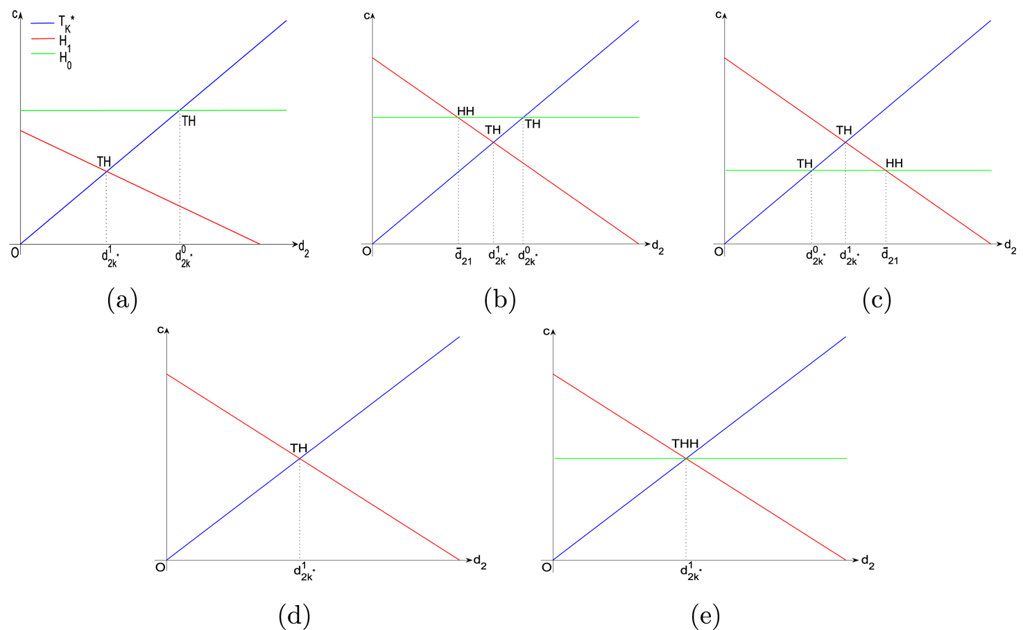Moreover, the real parts of other eigenvalues for the characteristic equation (4.3) are negative except for a pair of purely imaginary eigenvalues and a simple zero eigenvalue, where $k^*$, $k_0$, $d^1_{2k^*}$, and $c^1_{k^*}$ are given in (4.9), (4.10), (4.13), and (4.23), respectively (see figure 14(d)).

Figure 14.

Turing–Hopf, double-Hopf, and Turing–double-Hopf bifurcations of system (1.3) near $E_*$ in the $(d_2,\,c)$-plane for any $l>0$: (a) $(a,\,b,\,e,\,u_*)\in {U}_{32}$ and $u_* l^2\leq d_1< s_1 l^2$; (b) $(a,\,b,\,e,\,u_*)\in {U}_{32}$, $0< d_1< u_* l^2$ and $d^0_{2k^*}>\bar {d}_{21}$; (c) $(a,\,b,\,e,\,u_*)\in {U}_{32}$, $0< d_1< u_* l^2$ and $d^0_{2k^*}<\bar {d}_{21}$; (d) $(a,\,b,\,e,\,u_*)\in {U}_{31}$; (e) $(a,\,b,\,e,\,u_*)\in {U}_{32}$ and $d^0_{2k^*}=\bar {d}_{21}$. $H_0$, $H_1$, and $T_{k^*}$ represent the $0$-mode, $1$-mode Hopf bifurcation, and $k^*$-mode Turing bifurcation curves, respectively. $TH$, $HH$, and $THH$ represent Turing–Hopf bifurcation, double-Hopf bifurcation, and Turing–double-Hopf bifurcation, respectively.

Proof. By lemma 4.2, we know that there is no $0$-mode Hopf bifurcation if $(a,\,b,\,e,\,u_*)\in {U}_{31}$. The assumption $0< d_1< s_1 l^2$ guarantees that $\Gamma _1$ is nonempty. Let $c^H_1(d_2)=c^T_{k^*}(d_2)$, we can obtain the intersection of $H_1$ and $T_{k^*}$ is $(d^1_{2k^*},\,c^1_{k^*})$.

When $(d_2,\,c)=(d^1_{2k^*},\,c^1_{k^*})$, $\mathcal {T}_0(d^1_{2k^*},\,c^1_{k^*})<0$ for $(a,\,b,\,e,\,u_*)\in {U}_{31}$, and $\mathcal {T}_1(d^1_{2k^*},\,c^1_{k^*})=0$. Since $\mathcal {T}_k$ is decreasing in $k$, then for any $k\in \mathbb {N}$:

\[ \mathcal{T}_k(d^1_{2k^*},c^1_{k^*})<\mathcal{T}_1(d^1_{2k^*},c^1_{k^*})=0, \]

which implies that $\mathcal {T}_{k^*}(d^1_{2k^*},\,c^1_{k^*})<0$ as $k^*>1$. In addition, $\mathcal {M}_{k^*}(d^1_{2k^*},\,c^1_{k^*})=0$. Thus, $\mathcal {P}_{k^*}(\lambda )=0$ has a simple zero, and for any $k\neq 1$, $\mathcal {P}_{k}(\lambda )=0$ has no purely imaginary roots.

For any $k\in \Gamma _1$ and $k\neq k^*$, we have $c^1_{k^*}=c^H_1(d^1_{2k^*})=c^T_{k^*}(d^1_{2k^*})>c^T_{k}(d^1_{2k^*})$, then according to lemma 4.1(2) and $c^T_{k_0}\neq c^T_{k_0+1}$, $\mathcal {M}_k(d^1_{2k^*},\,c^1_{k^*})>0$ holds for each $k\in \Gamma _1$ and $k\neq k^*$. Since $k^*>1$, then $\mathcal {M}_1(d^1_{2k^*},\,c^1_{k^*})>0$. By lemma 4.1(1), $\mathcal {M}_k(d^1_{2k^*},\,c^1_{k^*})>0$ for any $k\notin \Gamma _1$. Hence, $\mathcal {P}_1(\lambda )=0$ has a pair of purely imaginary roots, and for any $k\neq k^*$, $\mathcal {P}_k(\lambda )=0$ has no zero eigenvalue.

Moreover, according to (4.15) and (4.22) the transversality conditions are fulfilled. Therefore, system (1.3) undergoes a $(k^*,\,1)$-mode Turing–Hopf bifurcation near positive constant steady state $E_*$ at $(d_2,\,c)=(d^1_{2k^*},\,c^1_{k^*})$.

Remark 4.11 When $k^*=1$, a Bogdanov–Takens bifurcation may occur. To reduce the length of the paper, we ignore the case $k^*=1$.

Theorem 4.12 For any $l>0$ and $(a,\,b,\,e,\,u_*)\in {U}_{32}$, assume that $0< d_1< s_1 l^2$, $k^*>1$, and $c^T_{k_0}\neq c^T_{k_0+1}$, then the following statements hold:

(1) if $u_* l^2\leq d_1< s_1 l^2$, system (1.3) undergoes a $(k^*,\,0)$-mode Turing–Hopf bifurcation near constant steady state $E_*$ at $(d^0_{2k^*},\,c^0_{k^*})$.
(2) if $0< d_1< u_* l^2$, then we have the following result:
1. (i) when $d^0_{2k^*}>\bar {d}_{21}$, then system (1.3) undergoes a $(k^*,\,0)$-mode Turing–Hopf bifurcation near constant steady state $E_*$ at $(d^0_{2k^*},\,c^0_{k^*})$;
2. (ii) when $d^0_{2k^*}<\bar {d}_{21}$, then system (1.3) undergoes a $(k^*,\,1)$-mode Turing–Hopf bifurcation near constant steady state $E_*$ at $(d^1_{2k^*},\,c^1_{k^*})$.

Moreover, the real parts of other eigenvalues for the characteristic equation (4.3) are negative except for a pair of purely imaginary eigenvalues and a simple zero eigenvalue. Here, $d^1_{2k^*}$, $d^0_{2k^*}$, $\bar {d}_{21}$, $c^1_{k^*}$, and $c^0_{k^*}$ are given in (4.13), (4.17), (4.20), and (4.23), respectively.

Proof. (1) As $(a,\,b,\,e,\,u_*)\in {U}_{32}$, then $c^H_0>0$. Let $c^H_0=c^H_{k^*}$, we obtain the intersection of $H_0$ and $T_{k^*}$, given by $(d^0_{2k^*},\,c^0_{k^*})$, and $(d^0_{2k^*},\,c^0_{k^*})$ is above $(d^1_{2k^*},\,c^1_{k^*})$ in the $(d_2,\,c)$-plane. When $(d_2,\,c)=(d^0_{2k^*},\,c^0_{k^*})$, $\mathcal {T}_0(d^0_{2k^*},\,c^0_{k^*})=0$. If $u_* l^2\leq d_1< s_1 l^2$, then $\mathcal {T}_1(d^0_{2k^*},\,c^0_{k^*})=-v_*c^0_{k^*}+s_1-{{d}_1}/{l^2}-{{d}^0_{2k^*}}/{l^2}=u_* l^2-{{d}_1}/{l^2}-{{d}^0_{2k^*}}/{l^2}<0$. Since $\mathcal {T}_k$ is decreasing in $k$, then for any positive integer $k$, $\mathcal {T}_k(d^0_{2k^*},\,c^0_{k^*})\leq \mathcal {T}_1(d^0_{2k^*},\,c^0_{k^*})<0$ hold, which implies that $\mathcal {T}_{k^*}(d^0_{2k^*},\,c^0_{k^*})<0$. On the other hand, for $(d_2,\,c)=(d^0_{2k^*},\,c^0_{k^*})$, $\mathcal {M}_{k^*}(d^0_{2k^*},\,c^0_{k^*})=0$. Hence, $\mathcal {P}_{k^*}(\lambda )=0$ has a simple zero, and for any $k\neq 0$, $\mathcal {P}_k(\lambda )=0$ has no purely imaginary roots.

For any $k\notin \Gamma _1$, by lemma 4.1(1), $\mathcal {M}_k(c)>0$ for any $c>0$, thus ${\mathcal {M}_k(d^0_{2k^*},\,c^0_{k^*})>0}$, and we also have $\mathcal {M}_0(d^0_{2k^*},\,c^0_{k^*})>0$. When $k^*>1$ and $c^T_{k_0}\neq c^T_{k_0+1}$, by the definition of $k^*$, we have $c^0_{k^*}=c^H_0=c^T_{k^*}(d^0_{2k^*})\geq c^T_k(d^0_{2k^*})$ for any $k\in \mathbb {N}$, then $\mathcal {M}_k(d^0_{2k^*},\,c^0_{k^*})>0$ for $k\in \Gamma _1$ and $k\neq k^*$, which implies that $\mathcal {P}_0(\lambda )=0$ has a pair purely imaginary roots, and for any $k\neq k^*$, $\mathcal {P}_k(\lambda )=0$ has no zero eigenvalue. Moreover, the transversality conditions hold via (4.19) and (4.22). Hence, system (1.3) undergoes a $(k^*,\,0)$-mode Turing–Hopf bifurcation at $(d_2,\,c)=(d^0_{2k^*},\,c^0_{k^*})$.

(2) If $0< d_1< u_* l^2$, then $H_0$ and $H_1$ intersect at $(d_2,\,c)=(\bar {d}_{21},\,c^H_0)$. According to the relationship between $\bar {d}_{21}$ and $d^0_{2k^*}$, we have the following two cases:

(i) if $\bar {d}_{21}< d^0_{2k^*}$, then $(d^0_{2k^*},\,c^0_{k^*})$ is above $(d^1_{2k^*},\,c^1_{k^*})$ in the $(d_2,\,c)$-plane, see figure 14(b);
(ii) if $\bar {d}_{21}>d^0_{2k^*}$, then $(d^0_{2k^*},\,c^0_{k^*})$ is below $(d^1_{2k^*},\,c^1_{k^*})$ in the $(d_2,\,c)$-plane, see figure 14(c).

Case (2) can be proved by using the same argument as in the proofs of theorem 4.10 and case (1).

Corollary 4.13 For any $l>0$ and $(a,\,b,\,e,\,u_*)\in {U}_{32}$, assume that $0< d_1< s_1 l^2$, $k^*>1$, and $c^T_{k_0}\neq c^T_{k_0+1}$, then system (1.3) undergoes a $(k^*,\,1,\,0)$-mode Turing–double-Hopf bifurcation near the constant steady state $E_*$ at $(d^1_{2k^*},\,c^1_{k^*})$, when $d^0_{2k^*}=\bar {d}_{21}$. Moreover, the real parts of other eigenvalues for the characteristic equation (4.3) are negative except for two pairs of purely imaginary eigenvalues and a simple zero eigenvalue (see figure 14(e)).

4.3. Spatiotemporal patterns via double-Hopf bifurcation

In this subsection, we use the formulas derived by Geng and Wang [Reference Geng and Wang13] to compute the $(0,\,1)$-mode double-Hopf bifurcation normal form, which may help us to find some interesting spatiotemporal patterns. Let:

\[ d_2=\bar{d}_{21}+\eta_1,\quad c=c^H_0+\eta_2, \]

where $\bar {d}_{21}$ and $c^H_0$ are given in (4.20) and (4.16), respectively. Define:

\[ V(t)=(u(t),v(t))^T, \quad \hat{V}(t)=\frac{1}{l\pi}\int\nolimits_{0}^{l\pi}V(y,t)\,{\rm d}y, \]

and system (1.3) can be transformed into:

(4.24)\begin{equation} \dot{V}(t)=D_0(\eta)\Delta{V}(t)+L(\eta)V(t)+\hat{L}(\eta)\hat{V}(t)+G(V(t),\hat{V}(t),\eta), \end{equation}

in which

\begin{align*} & {D(\eta)}={\left(\begin{array}{@{}cc@{}} d_{1} & 0\\ 0 & \bar{d}_{21}+\eta_1\end{array}\right),}\\ & \begin{array}{ll} L(\eta)=\begin{pmatrix} s_{1} & -\displaystyle\dfrac{b u_*}{a+u_*}\\ \displaystyle\dfrac{aev_*}{(a+u_*)^2}c^H_0 & -v_* c^H_0 \end{pmatrix},\quad \hat{L}(\eta)=\begin{pmatrix} -u_{*} & 0 \\ 0 & 0 \end{pmatrix}, \end{array}\\ & {G({\bf u},\hat{{\bf u}},\eta)}={\left(\begin{array}{@{}cc@{}} (u+u_*)(1-\hat{u}-u_*)-\displaystyle\dfrac{b(u+u_*)(v+v_*)}{a+u+u_*}+u_*\hat{u}-s_1 u_1+\dfrac{b u_*}{a+u_*}v\\ (c^H_0+\eta_2)(v+v_*)\bigg(1-v-v_*+\displaystyle\dfrac{e(u+u_*)}{a+u+u_*}\bigg)-(c^H_0+\eta_2)\bigg(\dfrac{aev_*}{(a+u_*)^2}u-v_* v\bigg)\end{array}\!\!\!\right),} \end{align*}

and ${\bf u}=(u,\,v)^T$, $\hat {{\bf u}}=(\hat {u},\,\hat {v})^T:=({1}/{l\pi })\int \nolimits _{0}^{l\pi }{\bf u}(\zeta,\,t){\rm d}\zeta$, $\eta =(\eta _1,\,\eta _2)$. Then

\begin{align*} & D_0(\eta)=\begin{pmatrix} d_{1} & 0\\ 0 & \bar{d}_{21} \end{pmatrix},\quad D_1(\eta)=\begin{pmatrix} 0 & 0 \\ 0 & \eta_1 \end{pmatrix},\\ & \begin{array}{ll} L_0=\begin{pmatrix} s_{1} & -\displaystyle\dfrac{b u_*}{a+u_*}\\ \displaystyle\dfrac{aeu_*(1-u_*)}{(a+u_*)^2}c^H_0 & -v_* c^H_0 \end{pmatrix},\quad L_1(\eta)=\begin{pmatrix} 0 & 0 \\ \displaystyle\dfrac{aeu_*}{(a+u_*)^2}\eta_2 & -v_*\eta_2 \end{pmatrix}, \end{array}\\ & \begin{array}{ll} \hat{L}(0)(\eta)=\begin{pmatrix} -u_{*} & 0\\ 0 & 0 \end{pmatrix},\quad \hat{L}_1(\eta)=\begin{pmatrix} 0 & 0 \\ 0 & 0 \end{pmatrix}, \end{array}\\ & {Q({\bf V},{\bf V})}={\left(\begin{array}{@{}cc@{}} \displaystyle\dfrac{2a(1-u_*)}{(a+u_*)^2}u^2-\dfrac{2ab}{(a+u_*)^2}u v-2 u_* u \hat{u} - \dfrac{2aev_*c^H_0}{(a+u_*)^3}u^2+\dfrac{2aec^H_0}{(a+u_*)^2}u v-2 c^H_0 v^2\end{array}\!\!\!\right),}\\ & {C({\bf V},{\bf V}, {\bf V})}={\left(\begin{array}{@{}cc@{}} -\displaystyle\dfrac{6a(1-u_*)}{(a+u_*)^3}u^3+\dfrac{6ab}{(a+u_*)^3}u^2 v\\ \displaystyle\dfrac{6aev_*c^H_0}{(a+u_*)^4}u^3-\dfrac{6aec^H_0}{(a+u_*)^3}u^2 v\end{array}\!\!\!\right),} \end{align*}

where ${\bf V}={(\begin{array}{cc}{\bf u}\\ \hat {{\bf u}}\end{array})}$. For the $(0,\,1)$-mode double-Hopf bifurcation, according to [Reference Geng and Wang13], the eigenfunctions $\phi _1$, $\bar {\phi }_i$, $\psi _1$, $\bar {\psi }_i$ ($i=1,\,2$) satisfying $\psi _i\phi _i=1$, $\psi _i\phi _j=1$ for $i, j=1,\,2$ ($j\neq i$) are

\[ \begin{array}{ll} \phi_1=\begin{pmatrix} 1\\ \phi_{12} \end{pmatrix},\quad \phi_2=\begin{pmatrix} 1\\ \phi_{22} \end{pmatrix},\quad \psi_1=\begin{pmatrix} \displaystyle\dfrac{1}{N_1}\\ \displaystyle\dfrac{\psi_{12}}{N_1} \end{pmatrix}^T,\quad \psi_2=\begin{pmatrix} \displaystyle\dfrac{1}{N_2}\\ \displaystyle\dfrac{\psi_{22}}{N_2} \end{pmatrix}^T, \end{array} \]

where

\begin{align*} \phi_{12}& =\frac{(a+u_*)(s_1-u_*- {\rm i}\omega_1)}{bu_*},\quad \phi_{22}=\frac{(a+u_*)(s_1-{\rm i}\omega_2-{{d}_1}/{l^2})}{bu_*},\\ \psi_{12}& ={-}\frac{bu_*}{(a+u_*)({\rm i}\omega_1+c^H_0 v_*)},\quad \psi_{22}={-}\frac{bu_*}{(a+u_*)({\rm i}\omega_2+c^H_0 v_*+{\bar{d}_{21}}/{l^2})},\\ N_1& =1+\phi_{12}\psi_{12},\quad N_2=1+\phi_{22}\psi_{22}. \end{align*}

Next, we fix the parameters of (1.3) except $d_2$, $c$ as follows:

\[ a=0.5,\quad b=0.25,\quad e=5.9375,\quad d_1=0.5,\quad l=3. \]

For $(k_1,\,k_2)=(0,\,1)$, according to Lemma 3.4 and Proposition 3.5 in [Reference Geng and Wang13], we have the following statements.

Proposition 4.14 For system (1.3) with $(d_1,\,a,\,b,\,e,\,l)=(0.5,\,0.5,\,0.25,\,5.9375,\,3)$, the positive constant steady state $E_*$ is $(0.125,\,2.1875)$, and there exist critical values $(\bar {d}_{21},\,c^H_0,\,\omega _1,\,\omega _2)\doteq (0.625,\,0.02286,\,0.1285,\,0.03762)$ such that when $(d_2,\,c)=(\bar {d}_{21},\,c^H_0)$, all eigenvalues of $\mathcal {P}_k(\lambda )$ have negative real parts other than two pairs of purely imaginary roots $\pm {\rm i}\omega _1$, $\pm {\rm i}\omega _2$, and system (1.3) undergoes a $(0,\,1)$-mode double-Hopf bifurcation near $E_*$.

By Lemma 3.4 and Proposition 3.5 in [Reference Geng and Wang13], the coefficients of the normal form up to third order are as follows:

(4.25)\begin{align} a_1(\eta)& ={-}(1.09375-2.80989{\rm i})\eta_2 ,\nonumber\\ b_2(\eta)& ={-}(0.055556+0.1756399{\rm i})\eta_1-(1.09375-7.57567{\rm i})\eta_2,\nonumber\\ a_{2100}& ={-}1.28834-3.135{\rm i}, \quad a_{1011}={-}21.5985-41.8235{\rm i},\nonumber\\ b_{0021}& =10.0251-6.5363{\rm i}, \quad b_{1110}= 28.6488+141.7397{\rm i}, \end{align}

by making the following transformations successively:

\begin{align*} & z_1=r_1\cos(\theta)+{\rm i}r_1\sin(\theta),\quad z_2=r_2\cos(\theta)+{\rm i}r_2\sin(\theta);\\ & \sqrt{|{\rm Re}(a_{2100})|}{\rm sign}({\rm Re}(a_{2100}) r_1\rightarrow r_1, \enspace \sqrt{|{\rm Re}(b_{0021})|}r_2\rightarrow r_2,\enspace {\rm sign}({\rm Re}(a_{2100}))t\rightarrow t, \end{align*}

then the corresponding planar system is

(4.26)\begin{align} \dot{r}_1& = r_1(1.09375\eta_2+r^2_1-2.1545r^2_2),\nonumber\\ \dot{r}_2& = r_2(0.0555556\eta_1+1.09375\eta_2-22.237r^2_1-r^2_2), \end{align}

and all equilibria of system (4.26) are

\begin{align*} E_0& =(0,0),\quad E_1=(\sqrt{-1.0938\eta_2},0),\ {\rm for} \ \eta_2<0,\\ E_2& =(0,\sqrt{0.055556\eta_1+1.0938\eta_2}),\ {\rm for}\ \eta_2>{-}0.050794\eta_1,\\ E_3& =(\sqrt{0.002447\eta_1+0.02582\eta_2},\sqrt{0.001136 \eta_1+0.5197 \eta_2}),\\ & \quad {\rm for}\ 0.002447\eta_1+0.02582\eta_2>0\ {\rm and}\ 0.001136 \eta_1+0.5197 \eta_2>0. \end{align*}

It follows from ${\rm Re}(a_{2100})=-1.28834<0$ that the Case VIII of the unfolding in Chapter 7 of [Reference Guckenheimer and Holmes16] occurs. The critical bifurcation lines in the $(d_2,\,c)$-plane are as follows:

(4.27)\begin{align} & H_0: c=c^H_0,\quad H_1: c=c^H_0-0.050794(d_2-\bar{d}_{21}),\nonumber\\ & L_1: c=c^H_0-0.09479(d_2-\bar{d}_{21}), \quad d_2<\bar{d}_{21},\nonumber\\ & L_2: c=c^H_0-0.002186(d_2-\bar{d}_{21}), \quad d_2>\bar{d}_{21}. \end{align}

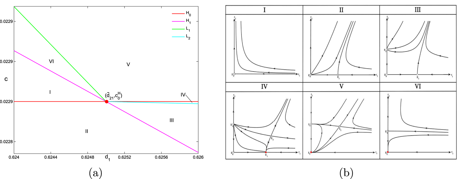
As shown in figure 15(a), the $(d_2,\,c)$-plane is divided into six disjoint regions around $(\bar {d}_{21},\,c^H_0)$, and the corresponding phase portraits are given in figure 15(b). The equilibria $E_0$, $E_{1}$, $E_2$, and $E_3$ of normal form system (4.26) corresponding to the positive constant steady state, the spatially homogeneous periodic solution, the spatially nonhomogeneous periodic solution, and spatially nonhomogeneous quasi-periodic solution of system (1.3), respectively. Thus, the dynamics of system (1.3) near the $(0,\,1)$-mode double-Hopf bifurcation singularity in the $(d_2,\,c)$-plane can be classified as follows:

(1) When $(d_2,\,c)\in \mathrm {I}$, $E_*$ is unstable.
(2) When $(d_2,\,c)\in \mathrm {II}$, $E_*$ remain unstable, and an unstable spatially homogeneous periodic solution $\bar {E}_1$ bifurcates from $E_*$.
(3) When $(d_2,\,c)\in \mathrm {III}$, $E_*$, and the spatially homogeneous periodic solution $\bar {E}_1$ are unstable, and an unstable spatially nonhomogeneous periodic solution $\bar {E}_2$ appears.
(4) When $(d_2,\,c)\in \mathrm {IV}$, $E_*$, and the spatially homogeneous periodic solution $\bar {E}_1$ are unstable, the spatially nonhomogeneous periodic solution $\bar {E}_2$ becomes locally asymptotically stable, and an unstable spatially nonhomogeneous quasi-periodic solution $\bar {E}_3$ appears.
(5) When $(d_2,\,c)\in \mathrm {V}$, $E_*$ becomes locally asymptotically stable, the spatially homogeneous periodic solution $\bar {E}_2$ becomes unstable, the quasi-periodic solution $\bar {E}_3$ remain unstable, and there is no spatially homogeneous periodic solution $\bar {E}_1$.
(6) When $(d_2,\,c)\in \mathrm {VI}$, $E_*$ remains locally asymptotically stable, the spatially nonhomogeneous quasi-periodic solution $\bar {E}_3$ disappears, and the spatially nonhomogeneous periodic solution $\bar {E}_2$ still unstable.

Figure 15.

(a) Bifurcation set of system (4.26) near $(\bar {d}_{21},\,c^H_0)$ in the $(d_2,\,c)$-plane. (b) The corresponding phase portraits in I–VI, where $H_0$, $H_1$, $L_1$, and $L_2$ represent critical bifurcation curves defined as in (4.27).

5. Concluding remarks

In this paper, we formulated and rigorously studied a host–parasitoid model with generalist predation and diffusion, where the predators have alternative food. After performing a detailed bifurcation analysis, our results revealed that system (1.3) exhibits complex dynamics and rich bifurcations. For a local model, we provided some preliminary analysis on Hopf bifurcation. For a reaction–diffusion model with local intraspecific prey competition, we first obtained the Turing instability of spatially homogeneous steady states or spatially homogeneous periodic solutions. Then, we showed that the model with diffusion undergoes Hopf bifurcation and Turing–Hopf bifurcation. Especially, we found two different normal forms for the Turing–Hopf bifurcation, where a pair of spatially nonhomogeneous periodic solutions is stable for a (8,0)-mode Turing–Hopf bifurcation and unstable for a (3,0)-mode Turing–Hopf bifurcation. Our results indicate that the model exhibits complex pattern formations, including transient states (spatially homogeneous or nonhomogeneous periodic solutions), monostability (a spatially nonhomogeneous steady state or a spatially homogeneous periodic solution), bistability (a pair of spatially nonhomogeneous steady states or a pair of spatially nonhomogeneous periodic solutions), tristability (a pair of spatially nonhomogeneous steady states and a spatially homogeneous periodic solution), and heteroclinic orbits (connecting a spatially nonhomogeneous periodic solution to a non-constant steady state or a spatially homogeneous periodic solution, connecting a spatially homogeneous periodic solution to non-constant steady states and vice versa). Finally, numerical simulations are provided to illustrate complex dynamics and verify our theoretical results.

It is worth noting that we found two kinds of normal forms with different dynamics for Turing–Hopf bifurcation (see § 3), i.e. the (8,0)-mode Turing–Hopf bifurcation with a pair of stable spatially nonhomogeneous periodic solutions, and the (3,0)-mode Turing–Hopf bifurcation with a pair of unstable spatially nonhomogeneous periodic solutions. These two are similar to the Cases Ia and Ib in section 7.5 of [Reference Guckenheimer and Holmes16]. Recently, although Turing–Hopf bifurcation and the corresponding spatiotemporal patterns are discussed in different systems (see [Reference Cao and Jiang5, Reference Jiang, An and Shi19, Reference Lu, Xiang, Huang and Wang24, Reference Shi and Ruan32, Reference Yang and Song41] and references therein), normal forms with different modes having different dynamics for Turing–Hopf bifurcation in an applied problem are rare (see [Reference Jiang, An and Shi19, Reference Jiang, Wang and Cao20]).

After replacing the local intraspecific prey competition by nonlocal intraspecific prey competition in diffusion model (1.3), we obtained more complex dynamics, such as (i) both $(k,\,0)$-mode and $(k,\,1)$-mode Turing–Hopf bifurcations can destabilize the constant equilibrium $E^{*}$, whereas in contrast only $(k,\,0)$-mode for system with local interactions; (2) nonlocal interaction can induce double-Hopf and Turing–double-Hopf bifurcations, while local interaction cannot; (3) when $k^*=1$, a 1-mode Bogdanov–Takens bifurcation may occur; and (4) double-Hopf bifurcation can induce a superposition of time-periodic solutions with different spatial modes.

The spatially nonhomogeneous periodic solutions are stable for some parameter values (according to the result of the (8,0)-mode Turing–Hopf bifurcation) and unstable for other parameter values (according to the result of the (3,0)-mode Turing–Hopf bifurcation), which implies that system (1.3) may have a degenerate spatially nonhomogeneous Hopf bifurcation around $E_{*}$. Moreover, our results in [Reference Xiang, Huang, Ruan and Xiao38] showed that the local system of (1.3) exhibits degenerate Hopf bifurcation with codimension up to 2 at $E_{*}$, then we can discuss Turing instability of degenerate spatially homogeneous periodic solutions. We leave these as open questions.

Acknowledgements

Research was partially supported by NSFC (No. 12231008), NSERC (RGPIN-2020-03911 and RGPAS-2020-00090) and NSF (DMS-2052648).

References

Andreu-Vaillo, F., Mazon, J. M., Rossi, J. D. and Toledo-Melero, J. J., Nonlocal Diffusion Problems, Mathematical Surveys and Monographs, Vol. 165 (American Mathematical Society, Providence, RI, 2010).CrossRef Google Scholar

Bates, P. W., On some nonlocal evolution equations arising in materials science, in ‘Nonlinear Dynamics and Evolution Equations’, H. Brunner, X.-Q. Zhao and X. Zou (eds.), Fields Institute Communications 48 (2006), 13–52.Google Scholar

Britton, N. F.. Aggregation and the competitive exclusion principle. J. Theor. Biol. 136 (1989), 57–66.CrossRef Google Scholar PubMed

Cantrell, R. S. and Cosner, C., Spatial Ecology via Reaction–Diffusion Equations, Wiley Series in Mathematical and Computational Biology (John Wiley & Sons, 2003).CrossRef Google Scholar

Cao, X. and Jiang, W.. Turing–Hopf bifurcation and spatiotemporal patterns in a diffusive predator–prey system with Crowley–Martin functional response. Nonlinear Anal. Real World Appl. 43 (2018), 428–450.CrossRef Google Scholar

Cao, X. and Jiang, W.. Double zero singularity and spatiotemporal patterns in a diffusive predator–prey model with nonlocal prey competition. Discrete Contin. Dyn. Syst. Ser. B 25 (2020), 3461–3489.CrossRef Google Scholar

Chen, S. and Yu, J.. Stability and bifurcation in predator–prey systems with nonlocal prey competition. Discrete Contin. Dyn. Syst. 38 (2018), 43–61.CrossRef Google Scholar

Du, Y. and Lou, Y.. Qualitative behavior of positive solutions of a predator–prey model: effects of saturation. Proc. R. Soc. Edinburgh Sect. A 131 (2001), 321–349.CrossRef Google Scholar

Erbach, A., Lutscher, F. and Seo, G.. Bistability and limit cycles in generalist predator–prey dynamics. Ecol. Complex 14 (2013), 48–55.CrossRef Google Scholar

Ermentrout, G. B. and Cowan, J. D.. Secondary bifurcation in neuronal nets. SIAM J. Appl. Math. 39 (1980), 323–340.CrossRef Google Scholar

Fagan, W. F., Lewis, M. A., Neubert, M. G. and Van Den Driessche, P.. Invasion theory and biological control. Ecol. Lett. 5 (2002), 148–157.CrossRef Google Scholar

Furter, J. and Grinfeld, M.. Local vs. nonlocal interactions in population dynamics. J. Math. Biol. 27 (1989), 65–80.CrossRef Google Scholar

Geng, D. and Wang, B.. Normal form formulations of double-Hopf bifurcation for partial functional differential equations with nonlocal effect. J. Differ. Equ. 309 (2022), 741–785.CrossRef Google Scholar

Gourley, S.. Travelling front solutions of a nonlocal Fisher equation. J. Math. Biol. 41 (2000), 272–284.CrossRef Google Scholar PubMed

Gourley, S. and Ruan, S.. Spatio-temporal delays in plankton models: local stability and bifurcations. Appl. Math. Comput. 145 (2003), 391–412.Google Scholar

Guckenheimer, J. and Holmes, P.. Nonlinear Oscillations, Dynamical Systems, and Bifurcations of Vector Fields (New York, Springer, 1983).CrossRef Google Scholar

Hanski, I., Hansson, L. and Henttonen, H.. Specialist predators, generalist predators and the microtine rodent cycle. J. Anim. Ecol. 60 (1991), 353–367.CrossRef Google Scholar

Hassard, B. D., Kazarinoff, N. D. and Wan, Y. H.. Theory and Application for Hopf Bifurcation (Cambridge, Cambridge University Press, 1981).Google Scholar

Jiang, W., An, Q. and Shi, J.. Formulation of the normal form of Turing–Hopf bifurcation in partial functional differential equations. J. Differ. Equ. 268 (2020), 6067–6102.CrossRef Google Scholar

Jiang, W., Wang, H. and Cao, X.. Turing instability and Turing–Hopf bifurcation in diffusive Schnakenberg system with gene expression time delay. J. Dyn. Differ. Equ. 31 (2019), 2223–2247.CrossRef Google Scholar

Lindström, T.. Qualitative analysis of a predator–prey system with limit cycles. J. Math. Biol. 31 (1993), 541–561.CrossRef Google Scholar

Liu, Z., Shen, Z., Wang, H. and Jin, Z.. Analysis of a diffusive SIR model with seasonality and nonlocal incidence of infections. SIAM J. Appl. Math. 79 (2019), 2218–2241.CrossRef Google Scholar

Lu, M., Huang, J. and Wang, H.. An organizing center of codimension four in a predator–prey model with generalist predator: from tristability and quadristability to transients in a nonlinear environmental change. SIAM J. Appl. Dyn. Syst. 22 (2023), 694–729.CrossRef Google Scholar

Lu, M., Xiang, C., Huang, J. and Wang, H.. Bifurcations in the diffusive Bazykin model. J. Differ. Equ. 323 (2022), 280–311.CrossRef Google Scholar

Madec, S., Casas, J., Barles, G. and Suppo, C.. Bistability induced by generalist natural enemies can reverse pest invasions. J. Math. Biol. 75 (2017), 543–575.CrossRef Google Scholar PubMed

Magal, C., Conser, C., Ruan, S. and Casas, J.. Control of invasive hosts by generalist parasitoids. Math. Med. Biol. 25 (2008), 1–20.CrossRef Google Scholar PubMed

Owen, M. R. and Lewis, M. A.. How predation can slow, stop or reverse a prey invasion. Bull. Math. Biol. 63 (2001), 655–684.CrossRef Google Scholar PubMed

Perko, L.. Differential Equations and Dynamical Systems (3rd ed., New York, Springer, 2006).Google Scholar

Ruan, S., Spatial–temporal dynamics in nonlocal epidemiological models, in ‘Mathematics for Life Science and Medicine’, Y. Takeuchi, K. Sato, and Y. Iwasa (eds.), (Springer-Verlag, Berlin, 2007, pp. 97–122).CrossRef Google Scholar

Schreiber, S. J.. On coexistence of species sharing a predator. J. Differ. Equ. 196 (2004), 209–225.CrossRef Google Scholar

Seo, G. and Wolkowicz, G. S. K.. Pest control by generalist parasitoids: a bifurcation theory. Discrete Contin. Dyn. Syst. Ser. S 13 (2020), 3157–3187.CrossRef Google Scholar

Shi, H. and Ruan, S.. Spatial, temporal and spatiotemporal patterns of diffusive predator–prey models with mutual interference. IMA J. Appl. Math. 80 (2015), 1534–1568.CrossRef Google Scholar

Shi, J., Wang, C. and Wang, H.. Diffusive spatial movement with memory and maturation delays. Nonlinearity 32 (2019), 3188–3208.CrossRef Google Scholar

Sun, G., Zhang, H., Chang, L., Jin, Z., Wang, H. and Ruan, S.. On the dynamics of a diffusive foot-and-mouth disease model with nonlocal infections. SIAM J. Appl. Math. 82 (2022), 1587–1610.CrossRef Google Scholar

van Leeuwen, E., Jansen, V. A. A. and Bright, P. W.. How population dynamics shape the functional response in a one-predator–two-prey system. Ecology 88 (2007), 1571–1581.CrossRef Google Scholar

Wang, H. and Salmaniw, Y.. Open problems in PDE models for knowledge-based animal movement via nonlocal perception and cognitive mapping. J. Math. Biol. 86 (2023), 71.CrossRef Google Scholar PubMed

Wu, S. and Song, Y.. Stability and spatiotemporal dynamics in a diffusive predator–prey model with nonlocal prey competition. Nonlinear Anal. Real World Appl. 48 (2019), 12–39.CrossRef Google Scholar

Xiang, C., Huang, J., Ruan, S. and Xiao, D.. Bifurcation analysis in a host–generalist parasitoid model with Holling II functional response. J. Differ. Equ. 268 (2020), 4618–4662.CrossRef Google Scholar

Xiang, C., Huang, J. and Wang, H.. Linking bifurcation analysis of Holling–Tanner model with generalist predator to a changing environment. Stud. Appl. Math. 149 (2022), 124–163.CrossRef Google Scholar

Xiao, D. and Zhang, K. F.. Multiple bifurcations of a predator–prey system. Discrete Contin. Dyn. Syst. Ser. B 8 (2007), 417–437.CrossRef Google Scholar

Yang, R. and Song, Y.. Spatial resonance and Turing–Hopf bifurcations in the Gierer–Meinhardt model. Nonlinear Anal. Real World Appl. 31 (2016), 356–387.CrossRef Google Scholar

Yi, F., Wei, J. and Shi, J.. Bifurcation and spatiotemporal patterns in a homogeneous diffusive predator–prey system. J. Differ. Equ. 246 (2009), 1944–1977.CrossRef Google Scholar

Zhao, G. and Ruan, S.. Spatial and temporal dynamics of a nonlocal viral infection model. SIAM J. Appl. Math. 78 (2018), 1954–1980.CrossRef Google Scholar

Figure 1. (a) $E_{*}$ of system (2.1) is stable when $c=\frac {1}{40}>c^{H}_0=\frac {4}{175}$; (b) $E_{*}$ of system (2.1) is unstable and surrounded by a stable limit cycle when $c=\frac {1}{50}< c^{H}_0$.

Figure 2. Turing instability of the spatially homogeneous steady state $E_*(u_*,\,v_*)$: (a) $l=1$, $E_{*}$ is stable with respect to systems (1.3); (b) $l=3$, $E_{*}$ is unstable with respect to system (1.3). $u_{0}(x)=\frac {1}{12}-0.001\cos (x),\, v_{0}(x)=\frac {77}{48}+0.001\cos (x)$.

Figure 3. Stable spatially homogeneous periodic solution bifurcating from 0-mode Hopf bifurcation in system (1.3), where $(a,\,b,\,e)=(\frac {1}{2},\,\frac {1}{3},\,\frac {7}{2})$, $l=2$, $(d_{1},\,d_{2})=(0.015,\,\frac {1}{3})$, $c=0.03< c^{H}=0.031$, $(u_{0}(x),\,v_{0}(x))=(0.1-0.01 \cos (1.5x),\,1.8-0.05\cos (1.5x))$.

Figure 4. Turing bifurcation curves $L_k,\, L_j,\, L_{k^{*}_{0}}$, Hopf bifurcation curve $H_0$ and Turing–Hopf bifurcation points $TH_k,\, TH_j,\, TH_{k^{*}_{0}}$ in the $(d_{1},\,c)$-plane.

Figure 5. $(3,\,0)$-mode Turing–Hopf bifurcation diagram in the $(d_{1},\,c)$-plane for system (1.3) and the corresponding phase portraits for system (3.22).

Figure 6. When $(d_{1},\,c)\in {\rm I}$ in figure 5(a) for the $(3,\,0)$-mode Turing–Hopf bifurcation, system (3.18) exhibits monostability: a positive constant steady state $E_{*}(0.109,\,1.629)$.

Figure 7. When $(d_{1},\,c)\in {\rm II}$ in figure 5(a) for the $(3,\,0)$-mode Turing–Hopf bifurcation, system (3.18) exhibits bistability: (a),(b) One spatially nonhomogeneous steady state and (c,d): the other spatially nonhomogeneous steady state.

Figure 8. When $(d_{1},\,c)\in {\rm III}$ in figure 5(a) for the $(3,\,0)$-mode Turing–Hopf bifurcation, system (3.18) exhibits an unstable spatially homogeneous periodic solution and bistability: (a, b) system (3.18) evolves from the transient spatially homogeneous periodic solution to one spatially nonhomogeneous steady stateand (c, d) to the other spatially nonhomogeneous steady state.

Figure 9. When $(d_{1},\,c)\in {\rm IV}$ in figure 5(a) for the $(3,\,0)$-mode Turing–Hopf bifurcation, system (3.18) exhibits a pair of unstable spatially nonhomogeneous periodic solutions and tristability: (a, b) transient spatially nonhomogeneous periodic solutions to a stable spatially homogeneous periodic solution, (c, d) one stable spatially nonhomogeneous steady state,and (e, f) the other stable spatially nonhomogeneous steady state.

Figure 10. When $(d_{1},\,c)\in {\rm V}$ in figure 5(a) for the $(3,\,0)$-mode Turing–Hopf bifurcation, a pair of unstable spatially nonhomogeneous periodic solutions disappear and system (3.18) exhibits monostability: a spatially homogeneous periodic solution.

Figure 11. When $(d_{1},\,c)\in {\rm VI}$ in figure 5(a) for the $(3,\,0)$-mode Turing–Hopf bifurcation, a pair of unstable spatially nonhomogeneous steady states disappear and system (3.18) exhibits monostability: a spatially homogeneous periodic solution.

Figure 12. Phase portrait of system (3.26) for the $(8,\,0)$-mode Turing–Hopf bifurcation when $(\mu _{1},\,\mu _{2})\in {\rm IV}$ in figure 5(a).

Figure 13. When $(d_1,\,c)\in {\rm IV}$ in figure 5(a) for the $(8,\,0)$-mode Turing–Hopf bifurcation, a spatially homogeneous steady state, a pair of spatially nonhomogeneous steady states and a spatially homogeneous periodic solution are all unstable, while a pair of spatially nonhomogeneous periodic solutions is stable: (a, b) one stable spatially nonhomogeneous periodic solution, (c, d) the other stable spatially nonhomogeneous periodic solution, where $u_{0}(x)=0.05\pm 0.03{\rm cos}(\frac {4}{3}x),\,\;v_{0}(x)=2.09-0.01{\rm cos}(\frac {4}{3}x)$, $(\mu _1,\,\mu _2)=(-0.001,\,-0.0006)$.

Figure 14. Turing–Hopf, double-Hopf, and Turing–double-Hopf bifurcations of system (1.3) near $E_*$ in the $(d_2,\,c)$-plane for any $l>0$: (a) $(a,\,b,\,e,\,u_*)\in {U}_{32}$ and $u_* l^2\leq d_1< s_1 l^2$; (b) $(a,\,b,\,e,\,u_*)\in {U}_{32}$, $0< d_1< u_* l^2$ and $d^0_{2k^*}>\bar {d}_{21}$; (c) $(a,\,b,\,e,\,u_*)\in {U}_{32}$, $0< d_1< u_* l^2$ and $d^0_{2k^*}<\bar {d}_{21}$; (d) $(a,\,b,\,e,\,u_*)\in {U}_{31}$; (e) $(a,\,b,\,e,\,u_*)\in {U}_{32}$ and $d^0_{2k^*}=\bar {d}_{21}$. $H_0$, $H_1$, and $T_{k^*}$ represent the $0$-mode, $1$-mode Hopf bifurcation, and $k^*$-mode Turing bifurcation curves, respectively. $TH$, $HH$, and $THH$ represent Turing–Hopf bifurcation, double-Hopf bifurcation, and Turing–double-Hopf bifurcation, respectively.

Figure 15. (a) Bifurcation set of system (4.26) near $(\bar {d}_{21},\,c^H_0)$ in the $(d_2,\,c)$-plane. (b) The corresponding phase portraits in I–VI, where $H_0$, $H_1$, $L_1$, and $L_2$ represent critical bifurcation curves defined as in (4.27).

Article contents

Bifurcations and pattern formation in a host–parasitoid model with nonlocal effect

Abstract

Keywords

MSC classification

Information

1. Introduction

2. Hopf bifurcation of the ODE system

3. System (1.3) with local intraspecific prey competition

3.1. Turing instability of the reaction–diffusion system

3.2. Bifurcations of the reaction–diffusion system

3.2.1. Hopf bifurcation.

3.2.2. Turing–Hopf bifurcation.

3.3. Spatiotemporal patterns via Turing–Hopf bifurcation

3.3.1. $(3,\,0)$-mode Turing–Hopf bifurcation.

3.3.2. $(8,\,0)$-mode Turing–Hopf bifurcation.

4. System (1.3) with nonlocal intraspecific prey competition

4.1. Hopf and double-Hopf bifurcation

4.2. Turing and Turing–Hopf bifurcations

4.3. Spatiotemporal patterns via double-Hopf bifurcation

5. Concluding remarks

Acknowledgements

References

Save article to Kindle

Save article to Dropbox

Save article to Google Drive

Reply to: Submit a response

Your details

You have entered the maximum number of contributors

Conflicting interests