



1 Introduction
A refined global and modal energy flow analysis is provided of a time-resolved three-dimensional (3D) turbulent wake from an experiment generalizing the frameworks of Rempfer & Fasel (Reference Rempfer and Fasel1994a ,Reference Rempfer and Fasel b ), Couplet, Sagaut & Basdevant (Reference Couplet, Sagaut and Basdevant2003) and Noack, Papas & Monkewitz (Reference Noack, Papas and Monkewitz2005). The modal decomposition aims to characterize the influence of the dynamics associated with coherent structures, which play an important role in turbulent flows. These large-scale structures underlie the mean flow, and thus aerodynamic forces via the Reynolds stress, and they feed the normal energy cascade towards dissipative small-scale structures via the production term. One exchange currency of these interactions is energy. Here, a modal decomposition is provided of the base-flow variation and the coherent structure of a highly modulated pyramid wake. The instantaneous and time-averaged energy flows between these modes, the mean flow and the unresolved fluctuations are deduced and quantified from the flow data. From the ensuing analysis, the contributions of the individual terms in the mean and turbulent kinetic energy balances can be studied. From a global perspective, this approach yields insights into the inter-modal transfer dynamics. A more detailed consideration of the local distributions of these terms can be linked to the principal flow features and thus, for example, an energy-based description of vortex interactions. More generally, the resulting analysis provides Navier–Stokes-based energy flow terms, as can be obtained from experimental particle image velocimetry (PIV) data and from unsteady Reynolds-averaged Navier–Stokes (URANS) simulations. For example, the modal energy or the relative importance of the individual energy balance terms can be compared directly. Thus, an energetic litmus test for the discrepancy between experiments and simulations is offered.
The modal energy interactions and nonlinear couplings are studied in the wake behind a wall-mounted low-aspect-ratio pyramid protruding through the boundary layer and with one face placed normal to the oncoming flow. The wake is described as turbulent with a highly 3D quasi-periodic flow. Such flows are of applied engineering interest. For example, these are representative of: the wake behind non-conventional buildings, affecting wind loading or urban comfort and safety; the influence of upstream mountain or rough terrain on the energy extraction potential of wind turbines; or mixing devices as found in combustors. More fundamentally, the bluff-body wake is a heuristic model for the study of large-scale coherent structures and vortex interaction dynamics.
The low-aspect-ratio wall-mounted pyramid flow shares similarities with that of the square-section finite cylinder counterpart. In both cases, the flow separates at the sharp leading edges and gives rise to a highly 3D turbulent wake to form a chain of linked vortex loops. The wake flow is characterized by strong quasi-periodic fluctuations, which are, unlike the case of the cantilevered circular cylinder (Okamoto & Sunabashiri Reference Okamoto and Sunabashiri1992; Adaramola et al. Reference Adaramola, Akinlade, Sumner, Bergstrom and Schenstead2006; Krajnović Reference Krajnović2011), strongly correlated over the entire height of the obstacle (McClean & Sumner Reference McClean and Sumner2012). For the cantilevered finite cylinder wakes, the periodicity can be attributed to the shedding of Kármán-type structures that are highly distorted due to the interactions with the separated shear layer at the free end and the boundary layer (Wang & Zhou Reference Wang and Zhou2009; Bourgeois, Sattari & Martinuzzi Reference Bourgeois, Sattari and Martinuzzi2011; Hosseini, Bourgeois & Martinuzzi Reference Hosseini, Bourgeois and Martinuzzi2013) in the wall–obstacle junction region. As the structures shed, the instantaneous location of the vortex centres in the region downstream of the obstacle tip lags those in the core region of the wake (Wang et al. Reference Wang, Zhou, Chan and Lam2006) to form a chain of linked vortex loops (Bourgeois et al. Reference Bourgeois, Sattari and Martinuzzi2011).
In comparison, the pyramid wake is even richer in vortex dynamics, due to the influence of the obstacle taper. Similarly to observations for wall-mounted triangular plates (Castro & Rogers Reference Castro and Rogers2002; Castro & Watson Reference Castro and Watson2004), the modulation of the wake fluctuation amplitude is much greater and there is a stronger low-frequency drift than is observed for cantilevered cylinder flows. Studies of the surface pressure distribution on the side faces of several low-aspect-ratio pyramids (AbuOmar & Martinuzzi Reference Abuomar and Martinuzzi2008; Martinuzzi Reference Martinuzzi2008) suggest important differences between the cylinder and pyramid flows. For both geometries, the dominant spectral peak of the surface pressure fluctuations matches the shedding frequency. For the cylinder, the fluctuations are in phase, within a small lag, over the entire side face. In contrast, the surface pressure fluctuations on the upper half are out of phase with those on the lower half of the pyramid face and the phase relation changes abruptly at about mid-height. Moreover, based on PIV measurements along planes normal to the flow, it was noted that an additional vortex was often present of similar strength to the vortices normally associated with the shedding process. From these observations, it was inferred that a second vortex forms near the tip region, referred to as the hairpin vortex based on its mean flow topology, which interacts with the shed structures forming in the base region – see, for example, figure 13 of Martinuzzi (Reference Martinuzzi2008). The interaction between these structures is believed to be closely linked to the dynamic behaviour observed in the pyramid wake. Hence, this work is a study of the inter-modal couplings and energy transfer mechanisms with the aim of better understanding the transient dynamics related to such interactions.
Intriguingly, key features of turbulent vortex shedding can be understood and modelled in the framework of weakly nonlinear stability analysis for the onset of the oscillatory instability. The onset of the vortex shedding in the prototypical cylinder wake is described with an instability of the Hopf bifurcation type, consisting of a pair of harmonic eigenmodes with a positive growth rate (unstable modes) and the remaining eigenmodes that are highly damped (stable modes) (Sreenivasan, Strykowski & Olinger Reference Sreenivasan, Strykowski, Olinger and Ghia1987; Schumm, Berger & Monkewitz Reference Schumm, Berger and Monkewitz1994). The transient dynamics are modelled using the mean-field ansatz, which consists of the steady solution, the unstable eigenmodes and a non-oscillatory mode that represents the mean-field deformation (Stuart Reference Stuart1971). The transient trajectory falls on a paraboloid in the phase space defined by the unstable pair and the non-oscillatory mode (Zielinska et al. Reference Zielinska, Goujon-Durand, Dušek and Wesfreid1997) as shown schematically in figure 1. The non-oscillatory mode is referred to as the shift mode, as it represents the shift of the short-time-averaged mean. Inclusion of the shift mode and its energy transfer with the harmonic pair is crucial in modelling the transient dynamics (Noack et al. Reference Noack, Afanasiev, Morzyński, Tadmor and Thiele2003). Interestingly, the cylinder wake transition from two-dimensional (2D) periodic vortex shedding to the 3D modes A and B is described by the coupled Landau model (Sheard, Thompson & Hourigan Reference Sheard, Thompson and Hourigan2003). Mathematically, this model is a generalization of the model describing the first bifurcation.
Schematic of the mean-field paraboloid in phase space:
 $a_{{\it\Delta}}$
and
 $a_{1},a_{2}$
correspond, respectively, to the amplitudes of the non-oscillatory mode and the fundamental harmonic pair.

The mean-field behaviour is also observed in the turbulent wake behind wall-mounted finite cylinders (Bourgeois, Noack & Martinuzzi Reference Bourgeois, Noack and Martinuzzi2013). Even in the presence of 3D effects, the global modes follow the mean-field paraboloid and a reduced-order model using the mean-field invariant manifold approximation successfully captures the main dynamics. For the current pyramid flow, however, the validity of mean-field theory cannot be assumed a priori given the existence of more complex interactions between multiple vortex structures. Whether the mean-field approximation in the presence of such nonlinear interactions is able to describe the prevalent dynamic behaviour has hitherto remained an open question.
The procedure enabling the analysis of the global flow field is based on earlier work. To isolate the coherent contribution and construct the global energetic modes, a modal subspace is defined based on the proper orthogonal decomposition (POD) following Bourgeois et al. (Reference Bourgeois, Noack and Martinuzzi2013) and Hosseini, Martinuzzi & Noack (Reference Hosseini, Martinuzzi and Noack2015). The POD provides an objective approach to educe the global modes in non-homogeneous flows and provides the natural basis to build the dynamical system of the coherent structures using a relatively small number of modes (cf. Tinney, Glauser & Ukeiley Reference Tinney, Glauser and Ukeiley2008a ). Here, the basis is carefully constructed using the benefits of the POD, appropriate choices of spatial filtering to incorporate the symmetry properties (Holmes et al. Reference Holmes, Lumley, Berkooz and Rowley2012) and to cleanly distil the base-flow variations and periodic modes. Such a basis is optimal in making an objective link to the physical mechanisms, as the basis modes can be associated with a physical interpretation.
In the following sections, a detailed modal energy analysis, based on the aforementioned basis modes, is performed to identify the sequence and direction of the energy flow among various scales of motion and to characterize the nonlinear couplings. The dataset includes time-resolved planar velocity measurements, synchronized with surface pressure measurements using a sensor-based estimation technique, taken for the wake behind a pyramid with apex angle
 ${\it\zeta}=60^{\circ }$
at a moderate Reynolds number of
 $28\,000$
. In § 2 the experimental set-up and flow conditions are described. The velocity modal decomposition and energy balance equations are summarized in § 3. In § 4 the detailed energy analysis for the considered flow are presented, followed by a summary of the main findings and concluding remarks in § 5. For self-consistency, the sensor-based estimation technique is summarized in appendix A.
2 Experimental set-up
The measurements were performed in an open-test-section suction-type wind tunnel schematically shown in figure 2 for the wake of a low-aspect-ratio pyramid with apex angle of
 ${\it\zeta}=60^{\circ }$
corresponding to a base width and height of
 $d=45~\text{mm}$
and
 $h=39~\text{mm}$
, respectively. The pyramid was mounted on a sharp-leading-edge flat plate with one face normal to the free stream. The free-stream velocity and Reynolds number were set to
 $U_{\infty }=10~\text{m}~\text{s}^{-1}$
and
 $Re_{d}=U_{\infty }d/{\it\nu}=28\,000$
, with a measured turbulence intensity of less than
 $0.8\,\%$
, where
 ${\it\nu}$
is the kinematic viscosity of air. The naturally developing boundary layer measured with laser Doppler velocimetry (LDV) (figure 3) follows a turbulent boundary layer profile and has a thickness of
 ${\it\delta}/h=0.25$
at the location of the pyramid. The origin is set at the centre of the pyramid base, with a Cartesian grid
 $\boldsymbol{x}=(x,y,z)$
defined as in figure 2. The
 $x$
-axis is aligned with the oncoming flow and the
 $z$
-axis is parallel to the pyramid axis. The velocity
 $\boldsymbol{u}$
has components
 $u$
,
 $v$
and
 $w$
in the
 $x$
,
 $y$
and
 $z$
directions, respectively.
Schematic of the experimental set-up and configuration of the measurement planes. The pressure is taken at
 $z/h=0.22,0.45,0.68$
and
 $x/d=0$
on the pyramid side faces and at
 $x/d=1,1.5$
and
 $y/d=\pm 0.25$
on the boundary layer plate.

The boundary layer profile and root-mean-square streamwise velocity fluctuations at the location of the obstacle. The displacement thickness
 ${\it\delta}^{\ast }$
, momentum thickness
 ${\it\theta}$
and shape factor
 $H={\it\delta}^{\ast }/{\it\theta}$
are shown in the graph.

A high-frame-rate stereoscopic PIV system was used to measure three-component velocity vectors at 20
 $(x{-}y)$
planes in the range
 $0<z/d<1.27$
with a separation of
 $0.067d$
, spanning
 $0.8<x/d<2.3$
and
 $-0.8<y/d<0.8$
. The configuration of the experimental planes is shown schematically in figure 2. The PIV system includes (i) a 10 mJ per pulse Photonics Industries 527 nm Nd:YLF laser system forming a 2 mm thick laser sheet, (ii) Laskin nozzle nebulizers generating
 $1~{\rm\mu}\text{m}$
olive oil particles that were illuminated in the laser sheet, and (iii) two Photron Fastcam SA4 cameras of
 $1024\times 1024$
pixels. The PIV configuration and processing parameters were selected after a lengthy trial-and-error process. Close attention was paid to the effect of the camera angles, time separation for the image pairs, particle density and distribution.
For the present experiments, the cameras were mounted symmetrically at a
 $45^{\circ }$
angle to the laser sheet. Image pairs with a time separation of
 $18~{\rm\mu}\text{s}$
were taken at a sampling rate of
 $f_{s}=500~\text{Hz}$
capturing approximately 10 data points per shedding cycle. For each plane, results are reported for three 4 s long trials, with a total of 6000 image pairs spanning 600 shedding cycles being taken. The velocity vectors were processed using the LaVision DaVis 8.2 software, with interrogation windows of
 $32\times 32$
pixels with
 $50\,\%$
overlap giving a vector spacing of 1.2 mm (
 $0.027d$
). For these acquisition parameters, it was verified that peak locking did not occur. Data sequences containing more than 1 % ‘bad vectors’ were rejected. The estimated uncertainty (Westerweel Reference Westerweel2000) on individual vector measurements is
 ${\rm\Delta}u/U_{\infty }=\pm 0.025$
. Using this value and the maximum measured variance, over 600 independent cycles, the statistical uncertainty for the mean velocity components is estimated to be
 ${\rm\Delta}U/U_{\infty }=\pm 0.008$
within a 95 % confidence level. Individual trials were repeated if the mean velocity field did not satisfy the estimated uncertainty. Based on a similar analysis for the higher-order moments, the maximum uncertainty is estimated to be: for the Reynolds stresses,
 ${\rm\Delta}\overline{u_{i}^{\prime }u_{j}^{\prime }}/U_{\infty }^{2}\approx 0.001$
; for the triple correlations,
 ${\rm\Delta}\overline{u_{i}^{\prime }u_{j}^{\prime }u_{k}^{\prime }}/U_{\infty }^{3}\approx 0.0005$
; and for the mean-field gradients
 ${\approx}0.02U_{\infty }/h$
. Based on an error propagation method, the maximum uncertainty for the mean and turbulent kinetic energy transport terms was estimated and is reported in the pertinent figures.
The estimation of the global modes from the isolated planar measurements was performed using the fluctuating surface pressure,
 $p^{\prime }$
, as the sensor data. Ten high-speed AllSensors Corp. pressure sensors were placed at pyramid side faces (
 $z/h=0.22,0.45,0.68$
at either sides) and the flat plate (
 $x/d=1,1.5$
at
 $y/d=\pm 0.25$
). The pressure data taken at a rate of 10.24 kHz were low-pass-filtered at 210 Hz with an eighth-order Butterworth filter. To keep the phase unchanged, the filtering was performed a second time in the reverse order.
The flow variables are non-dimensionalized with the free-stream velocity
 $U_{\infty }$
, the fluid density
 ${\it\rho}$
and pyramid base width
 $d$
. The rectangular observation domain is denoted by
 ${\it\Omega}$
with boundaries of
 $\partial {\it\Omega}$
, and the time and temporal window length of the measurements are respectively denoted by
 $t$
and
 $\mathscr{T}$
.
Before proceeding to the energy flow analysis, a brief overview of the flow characteristics is provided. Samples of the mean flow field are shown for the planes
 $y=0$
and
 $z/h=0.23$
in figure 4. In the plane
 $z/h=0.23$
(
 $z/d=0.20$
), the in-plane
 $x,y$
components
 $U$
and
 $V$
are shown as vectors, while the
 $z$
component,
 $W$
, is represented as flooded isocontours. The markers ‘
 $\boldsymbol{\times }$
’ indicate locations at which time series, as discussed below, are extracted. The mean field shows mirror symmetry about the plane
 $y=0$
to within the experimental uncertainty. The
 $W$
component is comparable in magnitude to the
 $V$
component over much of the wake, emphasizing the 3D nature of the wake. In the symmetry plane
 $y=0$
,
 $V=0$
and the
 $U,W$
vectors are shown together with the flooded isocontours representing
 $\overline{u^{\prime }w^{\prime }}$
. These Reynolds stresses are largest in regions of large gradients in
 $W$
, as is seen towards the tip region of the wake. In both planes, the mean shear layer bounding the recirculation zone can be identified.
The Reynolds stresses, shown in figure 5 for the plane
 $z/h=0.23$
, also show mirror symmetry about
 $y=0$
. High values of
 $\overline{u^{\prime 2}}$
and
 $\overline{u^{\prime }v^{\prime }}$
are concentrated along the shear layers, while those for
 $\overline{u^{\prime 2}}$
, indicating the end of the formation region, are concentrated immediately downstream of the mean recirculation region. Higher values of
 $\overline{w^{\prime 2}}$
are concentrated in the base region. In this plane,
 $\overline{u^{\prime }w^{\prime }}$
and
 $\overline{v^{\prime }w^{\prime }}$
are typically 2–3 times smaller than those for
 $\overline{u^{\prime }v^{\prime }}$
and are thus not negligible, but are not shown for brevity. Larger magnitudes of Reynolds stress containing
 $w^{\prime }$
fluctuations are generally observed along the shear layer in the tip region as seen, for example, in figure 4.
Mean velocity field along the symmetry plane
 $y=0$
and in the plane
 $z/h=0.23$
(
 $z/d=0.20$
). In the plane
 $y=0$
,
 $V=0$
and the in-plane vectors represent
 $U$
and
 $W$
components. The coloured isocontours represent
 $\overline{u^{\prime }w^{\prime }}$
. In the plane
 $z/h=0.23$
, vectors show the in-plane components
 $U$
and
 $V$
, while the out-of-plane
 $W$
component is shown as coloured isocontours. Points at which time series are extracted are indicated by ‘
 $\boldsymbol{\times }$
’. Flow is from left to right. For clarity, only every second vector is shown.

Coloured isocontours of the Reynolds stress field along the plane
 $z/h=0.23$
. Points at which time series are extracted are indicated by ‘
 $\boldsymbol{\times }$
’.

Spectra of the velocity fluctuations at the location
 $x/d=2.1,\,y/d=-0.3$
in the plane
 $z/h=0.23$
are shown in figure 6. A strong peak corresponding to the shedding frequency is observed for the two in-plane components. In contrast, the
 $w^{\prime }$
fluctuations appear only weakly correlated to the shedding process. The
 $w^{\prime }$
fluctuations, however, are more closely associated with the slowly varying base-flow fluctuations. As discussed in §§ 4 and 4.1, this association with the slowly varying base flow is maintained over the entire height of the pyramid. However, towards the tip region (typically
 $z/h>0.5$
), the
 $w^{\prime }$
fluctuations show a significant periodic component related to the passage of the shed vortices. Excerpts of the time sequences and the corresponding autocorrelation functions at the locations shown in figure 4 are shown in figure 7. The
 $u^{\prime }$
fluctuations remain correlated over a large number of cycles. Whereas for the points at
 $x/d=1.7$
and 2.3, the fluctuations are correlated with the shedding frequency, those for
 $x/d=1.3,\,y/d=0$
are correlated at twice the shedding frequency, suggesting that the second harmonic is locally important. For completeness, an excerpt of the
 $v^{\prime }$
fluctuations at
 $x/d=2.1,\,y/d=-0.3$
and its autocorrelation function is also shown in figure 7. These also illustrate a strong correlation over a large number of cycles.
Normalized power spectral density function (PSDF) for the three fluctuating velocity components at the location
 $x/d=2.1,\,y/d=-0.3$
in the plane
 $z/h=0.23$
. Here
 $f_{c}$
indicates the normalized shedding frequency. The PSDF is normalized by the signal variance.

Excerpts of the time series and autocorrelation functions,
 $R_{uu}$
, for the
 $u^{\prime }$
fluctuations at three locations (as indicated in the figure) in the plane
 $z/h=0.23$
. Also shown are
 $v^{\prime }$
and
 $R_{vv}$
at the location
 $x/d=2.1,\,y/d=-0.3$
in the plane
 $z/h=0.23$
. The time
 $t$
and temporal lag
 ${\it\tau}$
are in seconds.

Two-point cross-correlations for the
 $u^{\prime }$
and
 $v^{\prime }$
fluctuations are shown in figure 8. Within the observation domain, the fluctuations associated with the shed vortices are coherent, remaining strongly correlated in space over a large number of cycles. Also shown in figure 8 is a longitudinal spatial correlation function for
 $u^{\prime }$
along the line
 $y/d=-0.3$
. The observed wave form is consistent with the regular passage of large-scale coherent structures as associated with quasi-periodic vortex shedding.
(a,b) Two-point cross-correlation functions for
 $u^{\prime }$
and
 $v^{\prime }$
fluctuations in the plane
 $z/h=0.23$
between locations shown in the panels; the time lag
 ${\it\tau}$
is in seconds. (c) The longitudinal (spatial) cross-correlation function of
 $u^{\prime }$
as a function of the separation to the reference point,
 ${\rm\Delta}x$
, along
 $y/d=-0.3$
with the reference point at
 $x/d=2.1$
,
 $y/d=-0.3$
in the plane
 $z/h=0.23$
.

Spectra for the pressure fluctuations at two locations on the pyramid side faces and at a location on the wall in the pyramid wake are shown in figure 9. The peak associated with the shedding frequency is observed at all sensor locations. Note that, for the wake sensor, a weak energy accumulation at twice the shedding frequency can also be discerned. The times series excerpt and its autocorrelation function, also shown in figure 9, suggest that the pressure fluctuations also remain strongly correlated over a large number cycles.
(a) The normalized PSDF as a function of the normalized frequency for surface pressure measurements at two locations on the pyramid side face (at
 $x/d=0$
: red,
 $z/h=0.22$
; black,
 $z/h=0.45$
) and in the wall in the wake (blue,
 $x/d=1.0,\,y/d=-0.25$
). The PSDF are offset by
 $10^{3}$
for clarity. (b,c) An excerpt of the normalized pressure time series and its autocorrelation function,
 $R_{pp}$
, for the wake wall sensor.

3 Energy flow analysis
In this section, we propose a generalized modal energy flow analysis. First (§ 3.1), the construction of the modal expansion from PIV data is discussed. In § 3.2, time-averaged energy flow analysis is proposed. Finally, in § 3.3, refined instantaneous and inter-modal energy flows are presented.
The observation domain
 ${\it\Omega}$
is a rectangular volume, defined by the aforementioned measurement planes, behind the pyramid. The modal decomposition is based on the standard inner product between two square integrable velocity fields
 $\boldsymbol{u},\boldsymbol{v}\in \mathscr{L}^{2}({\it\Omega})$
:
 $$\begin{eqnarray}\displaystyle (\boldsymbol{u},\boldsymbol{v})_{{\it\Omega}}:=\int _{{\it\Omega}}\boldsymbol{u}\boldsymbol{\cdot }\boldsymbol{v}\,\text{d}\boldsymbol{x}, & & \displaystyle\end{eqnarray}$$
with the associated norm
 $\Vert \boldsymbol{u}\Vert _{{\it\Omega}}:=\sqrt{(\boldsymbol{u},\boldsymbol{ u})_{{\it\Omega}}}$
.
For later reference, we also introduce the time average for the velocity field
 $\boldsymbol{u}$
:
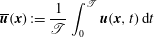 $$\begin{eqnarray}\displaystyle \overline{\boldsymbol{u}}(\boldsymbol{x}):=\frac{1}{\mathscr{T}}\int _{0}^{\mathscr{T}}\boldsymbol{u}(\boldsymbol{x},t)\,\text{d}t & & \displaystyle\end{eqnarray}$$
and analogously for other quantities. The integration period
 $\mathscr{T}$
is considered to be infinitely long, so that all moments can be considered as converged.
For the Navier–Stokes operations, we follow the notation of Noack, Morzyński & Tadmor (Reference Noack, Morzyński and Tadmor2011). The
 $\boldsymbol{{\rm\nabla}}$
and
 ${\rm\Delta}$
operators are defined as
 $\boldsymbol{{\rm\nabla}}:=(\partial _{x},\partial _{y},\partial _{z})$
and
 ${\rm\Delta}:=\partial _{xx}^{2}+\partial _{yy}^{2}+\partial _{zz}^{2}$
, where
 $\partial _{{\it\alpha}}$
and
 $\partial _{{\it\alpha}{\it\alpha}}^{2}$
denote the first and second partial derivatives with respect to
 ${\it\alpha}$
. The volume integral over the domain
 ${\it\Omega}$
is denoted as
 $(\unicode[STIX]{x1D641})_{{\it\Omega}}:=\int _{{\it\Omega}}\unicode[STIX]{x1D641}\,\text{d}\boldsymbol{x}$
and the surface integral as
 $[\unicode[STIX]{x1D641}]_{\partial {\it\Omega}}:=\oint _{\partial {\it\Omega}}\unicode[STIX]{x1D641}\boldsymbol{\cdot }\text{d}\boldsymbol{A}$
. Moreover, the Euclidean inner product is denoted by
 $\cdot$
, which contracts the inner indices. The double contraction
 $\boldsymbol{ : }$
for two matrices
 $\unicode[STIX]{x1D641}$
and
 $\unicode[STIX]{x1D642}$
reads
 $\unicode[STIX]{x1D641}\boldsymbol{ : }\unicode[STIX]{x1D642}=\sum _{{\it\alpha}=1}^{3}\sum _{{\it\beta}=1}^{3}F_{{\it\alpha}{\it\beta}}G_{{\it\beta}{\it\alpha}}$
, where
 ${\it\alpha}$
and
 ${\it\beta}$
are dummy variables over the Cartesian coordinates.
3.1 Three-dimensional modal expansion
In this section, we present the construction of an orthonormal Galerkin expansion of the 3D time-resolved velocity field from 2D PIV data. The starting point is the Reynolds decomposition of the velocity field into the mean
 $\boldsymbol{u}_{0}:=\overline{\boldsymbol{u}}$
and fluctuation
 $\boldsymbol{u}^{\prime }:=\boldsymbol{u}-\boldsymbol{u}_{0}$
, i.e.
 $$\begin{eqnarray}\displaystyle \boldsymbol{u}=\boldsymbol{u}_{0}+\boldsymbol{u}^{\prime }. & & \displaystyle\end{eqnarray}$$
The fluctuation is expanded with orthonormal modes
 ${\bf\phi}_{i}$
and corresponding temporal amplitudes
 $a_{i}$
. Following the elegant notation of Rempfer & Fasel (Reference Rempfer and Fasel1994b
), we express the velocity field by
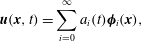 $$\begin{eqnarray}\displaystyle \boldsymbol{u}(\boldsymbol{x},t)=\mathop{\sum }_{i=0}^{\infty }a_{i}(t){\bf\phi}_{i}(\boldsymbol{x}), & & \displaystyle\end{eqnarray}$$
where the base flow has been included as the zeroth mode with
 $a_{0}\equiv 1$
. In practice, the expansion will be truncated after a finite number of modes
 $N$
, yielding a resolved part of the velocity field
 $$\begin{eqnarray}\displaystyle \boldsymbol{u}^{[0\ldots N]}(\boldsymbol{x},t)=\mathop{\sum }_{i=0}^{N}a_{i}(t){\bf\phi}_{i}(\boldsymbol{x}) & & \displaystyle\end{eqnarray}$$
and the residual
 $\boldsymbol{u}^{[N+1\ldots \infty ]}$
.
The 3D velocity fields are estimated from the planar velocity measurements and fluctuating surface pressure, obtained at the 10 locations identified in § 2, following the sensor-based estimation technique of Hosseini et al. (Reference Hosseini, Martinuzzi and Noack2015). To render a consistent flow topology and accurately represent the phase-space trajectory and transient dynamics of the coherent motions, the extended proper orthogonal decomposition (EPOD) technique (Borée Reference Borée2003) is modified in four respects. (1) The estimation basis is changed to an optimal orthonormal basis; the basis is carefully constructed by incorporating the symmetry properties (Holmes et al. Reference Holmes, Lumley, Berkooz and Rowley2012) and using appropriate choices of filtering, to distil the base-flow variations and harmonic oscillations. (2) The sensor history is used to recover velocity cyclical behaviour through the multi-time-delay approach (Durgesh & Naughton Reference Durgesh and Naughton2010). (3) The sensor-velocity phase difference for the non-harmonic mode is taken into account by including a time delay in the estimation found from peak of the pressure–velocity cross-correlation. (4) Finally, the estimation of the higher harmonics is improved using quadratic correlation terms. By including these improvements, the residual is significantly reduced and transient dynamics are recovered. The details of this procedure can be found in Hosseini et al. (Reference Hosseini, Martinuzzi and Noack2015) and a summary is provided for consistency in appendix A.
Tinney et al. (Reference Tinney, Glauser and Ukeiley2008a ) and Tinney, Ukeiley & Glauser (Reference Tinney, Ukeiley and Glauser2008b ) have laid out an alternative elegant spectral POD approach for state estimation. This approach solves problems (2)–(4) in a single algorithmic step. In this study, we chose to restrict the sensing data to a moving finite-time window to mitigate the effects of drifts and to prepare a causal framework for planned flow control experiments. The price of a causal estimation is the mentioned need to introduce parameters like the sampling frequency, the time horizon and the time delay. Similar parameters are, for instance, needed for ARMAX-based control (Hervé et al. Reference Hervé, Sipp, Schmid and Samuelides2012).
3.2 Time-averaged energy balance equations
The starting point of the energy balance equations is the Navier–Stokes equations in a steady domain
 ${\it\Omega}$
:
 $$\begin{eqnarray}\displaystyle \boldsymbol{R}[\boldsymbol{u}]:=\partial _{t}\boldsymbol{u}+\boldsymbol{{\rm\nabla}}\boldsymbol{\cdot }(\boldsymbol{u}\boldsymbol{u})-{\it\nu}{\rm\Delta}\boldsymbol{u}+\boldsymbol{{\rm\nabla}}p\equiv 0, & & \displaystyle\end{eqnarray}$$
where
 $\boldsymbol{R}$
denotes the Navier–Stokes residual,
 ${\it\nu}$
the kinematic viscosity, and
 $\boldsymbol{u}$
and
 $p$
respectively the velocity vector field and pressure. In writing the residual as a function of the velocity alone, the pressure is considered a function of the velocity field. This can be considered as a valid approximation for the considered steady domains with no-slip conditions on the ground and ambient flow at infinity. A trivial corollary of (3.6) is the weak form of the Navier–Stokes equation, i.e. that the projection of the Navier–Stokes residual on an arbitrary test function
 $\boldsymbol{v}$
vanishes,
 $$\begin{eqnarray}\displaystyle (\boldsymbol{v},\boldsymbol{R}[\boldsymbol{u}])_{{\it\Omega}}=0. & & \displaystyle\end{eqnarray}$$
In particular, the time-averaged projection of
 $\boldsymbol{R}$
on a potentially time-varying test function
 $\boldsymbol{v}$
vanishes, too:
 $$\begin{eqnarray}\displaystyle \overline{\left(\boldsymbol{v},\boldsymbol{R}[\boldsymbol{u}]\right)_{{\it\Omega}}}=0. & & \displaystyle\end{eqnarray}$$
The beauty of these corollaries is that most equations of the Galerkin method and of statistical fluid mechanics can be derived from (3.7) and (3.8). For example,
 $\boldsymbol{v}:={\bf\phi}_{i}$
and
 $\boldsymbol{u}=\sum _{i=0}^{N}a_{i}{\bf\phi}_{i}$
in (3.7) yields the Galerkin system
 $$\begin{eqnarray}\displaystyle \frac{\text{d}}{\text{d}t}a_{i}={\it\nu}\mathop{\sum }_{i=0}^{N}l_{ij}^{{\it\nu}}a_{i}+\mathop{\sum }_{j,k=0}^{N}q_{ijk}^{c}a_{j}a_{k}+\mathop{\sum }_{j,k=0}^{N}q_{ijk}^{p}a_{j}a_{k}, & & \displaystyle\end{eqnarray}$$
where the left-hand side represents the local acceleration,
 $l_{ij}^{{\it\nu}}=({\bf\phi}_{i},{\rm\Delta}{\bf\phi}_{j})_{{\it\Omega}}$
parametrizes the viscous term,
 $q_{ijk}^{c}=-({\bf\phi}_{i},\boldsymbol{{\rm\nabla}}\boldsymbol{\cdot }{\bf\phi}_{j}{\bf\phi}_{k})_{{\it\Omega}}$
originates from the convective term, and
 $q_{ijk}^{p}$
may arise from the pressure term (Noack et al.
Reference Noack, Papas and Monkewitz2005). For later reference, we introduce a convection Galerkin coefficient density
 $\tilde{q}_{ijk}^{c}$
as the integrand leading to
 $q_{ijk}^{c}$
,
 $$\begin{eqnarray}\displaystyle q_{ijk}^{c}=(\tilde{q}_{ijk}^{c})_{{\it\Omega}},\quad \text{where }\tilde{q}_{ijk}^{c}=-{\bf\phi}_{i}\boldsymbol{\cdot }\boldsymbol{{\rm\nabla}}\boldsymbol{\cdot }{\bf\phi}_{j}{\bf\phi}_{k}. & & \displaystyle\end{eqnarray}$$
Similarly, a drag or lift equation can be obtained from (3.8) with the unit vectors
 $\boldsymbol{e}_{x}$
and
 $\boldsymbol{e}_{y}$
as test functions pointing in the streamwise and orthogonal directions, respectively. Several other balance equations can be obtained (Noack et al.
Reference Noack, Morzyński and Tadmor2011).
In this study, we focus on the energy balance equations. Choosing
 $\boldsymbol{v}=\boldsymbol{u}$
in (3.8) yields the balance equation for the total mechanical energy. Exploiting the Reynolds decomposition
 $\boldsymbol{u}=\boldsymbol{u}_{0}+\boldsymbol{u}^{\prime }$
(3.3), this balance equation can be separated into a contribution for the mean flow energy
 $$\begin{eqnarray}\displaystyle K_{0}:=\Vert \boldsymbol{u}_{0}\Vert _{{\it\Omega}}^{2}/2 & & \displaystyle\end{eqnarray}$$
and one for the fluctuation
 $$\begin{eqnarray}\displaystyle K:=\Vert \overline{\boldsymbol{u}^{\prime }\boldsymbol{\cdot }\boldsymbol{u}^{\prime }}\Vert _{{\it\Omega}}^{2}/2. & & \displaystyle\end{eqnarray}$$
The first is obtained from (3.8) with the test function
 $\boldsymbol{v}=\boldsymbol{u}_{0}$
. This mean kinetic energy (MKE) equation has four terms: the convection of the MKE into the domain
 $C_{0}$
, the transfer to the fluctuations
 $T_{0}$
, the direct dissipation
 $D_{0}$
, and the mean pressure work,
 $F_{0}$
, i.e.
 $$\begin{eqnarray}\displaystyle 0=C_{0}+T_{0}+D_{0}+F_{0}. & & \displaystyle\end{eqnarray}$$
The terms on the right-hand side are given explicitly in table 1. The left-hand side
 $\overline{\text{d}K_{0}/\text{d}t}$
vanishes because we have assumed a sufficiently long integration period
 $\mathscr{T}$
.
Energy terms in the balance equations for mean flow
 $\boldsymbol{u}_{0}$
and fluctuation
 $\boldsymbol{u}^{\prime }$
.
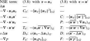
The second contribution is derived from (3.8) with the test function
 $\boldsymbol{v}=\boldsymbol{u}^{\prime }$
and is known as the turbulent kinetic energy (TKE) equation. This equation includes five terms: production
 $P$
, convection
 $C$
, transfer
 $T$
, dissipation
 $D$
and pressure work
 $F$
, i.e.
 $$\begin{eqnarray}\displaystyle 0=P+C+T+D+F. & & \displaystyle\end{eqnarray}$$
These terms are also summarized in table 1. Where applicable, the Gauss integral formula is implemented to reduce the volume integrals to surface integrals (Noack et al. Reference Noack, Afanasiev, Morzyński, Tadmor and Thiele2003).
We emphasize that the sum of (3.13) and (3.14) yields the total mechanical energy balance. Moreover, the TKE production results in a loss of mean energy,
 $$\begin{eqnarray}\displaystyle P=-T_{0}-[\overline{\boldsymbol{u}^{\prime }\boldsymbol{\cdot }\Vert \boldsymbol{u}^{\prime }\Vert ^{2}}]_{\partial {\it\Omega}} & & \displaystyle\end{eqnarray}$$
to within a small surface integral.
The TKE balance can be decomposed into modal contributions by starting with (3.8) but projecting on the modal fluctuation contribution
 $\boldsymbol{v}:=\boldsymbol{u}^{[i]}=a_{i}{\bf\phi}_{i}$
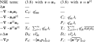
. The resulting modal energy flow equation (3.16) has analogous terms as (3.14), i.e. a modal production
 $P_{i}$
, convection
 $C_{i}$
, transfer
 $T_{i}$
, dissipation
 $D_{i}$
and pressure work
 $F_{i}$
(Noack et al.
Reference Noack, Papas and Monkewitz2005):
 $$\begin{eqnarray}\displaystyle 0=P_{i}+C_{i}+T_{i}+D_{i}+F_{i}. & & \displaystyle\end{eqnarray}$$
These terms are summarized in table 2 using
 ${\it\lambda}_{i}=\overline{a_{i}^{2}}$
. Table 2 also features the terms of the MKE equation exploiting the Galerkin expansion (3.4). Here, Galerkin coefficients are generalized for the projection on the mean flow, i.e.
 $i=0$
.
Energy terms in modal and base-flow balance equations.
3.3 Instantaneous modal energy flow analysis
In § 3.2, time-averaged energy equations have been discussed for the mean flow, the fluctuation and individual modes employing (3.8) for the projection on
 $\boldsymbol{v}=\boldsymbol{u}_{0}$
,
 $\boldsymbol{v}=\boldsymbol{u}^{\prime }$
and
 $\boldsymbol{v}=\boldsymbol{u}^{[i]}$
, respectively. Evidently, analogous instantaneous energy equations can be obtained by employing (3.7) instead of (3.8). We distinguish between averaged and instantaneous energy terms by omission or inclusion of ‘
 $(t)$
’ as argument, respectively. As will be shown in § 4.4 the instantaneous energy flows elucidate important inter-modal couplings that would be neglected by a time-averaged analysis.
Subsequently, we describe a detailed investigation of triadic interactions
 $T_{ijk}(t)=q_{ijk}^{c}a_{i}a_{j}a_{k}$
. Throughout the paper, in referring to the individual terms of the triadic interactions, the first harmonic pair modes are denoted by the subscript indices
 $i=1,2$
, the second pair modes by the indices
 $i=3,4$
, and the slow-drift mode by the index
 ${\it\Delta}$
. The energy transfer, however, occurs in groups as opposed to individual modes. These groups can consist of a large number of modes, making the representation cumbersome. Therefore, to simplify the notation, we group the modes based on their frequency content and study the energy transfer between the groups as opposed to individual modes. Based on the characteristics of the global modes (see § 4.1), three groups are considered:
-
(1) the first harmonic pair, which is an antisymmetric pair, denoted by the index
 $a$
;
-
(2) the second harmonic pair, which is a symmetric pair, denoted by the index
$s$
; and -
(3) the slow-drift mode, denoted by the index
${\it\Delta}$
.


The interactions between these three groups are represented by a total of six terms:
-
(i)
$T_{{\it\Delta}a}(t)$
,
$T_{a{\it\Delta}}(t)$
, transfer between the slow-drift mode and the antisymmetric pair; -
(ii)
$T_{sa}(t)$
,
$T_{as}(t)$
, transfer between the symmetric and antisymmetric pairs; -
(iii)
$T_{{\it\Delta}s}(t)$
,
$T_{s{\it\Delta}}(t)$
, transfer between the slow-drift mode and the symmetric pair.


Each term includes all the possible interactions between the two groups. For example,
 $T_{{\it\Delta}a}(t)$
is the sum of all the instantaneous inter-modal transfer terms
 $T_{ijk}(t)=q_{ijk}^{c}a_{i}a_{j}a_{k}$
with
 $i={\it\Delta}$
and at least one other index from group
 $a$
:
 $$\begin{eqnarray}\displaystyle T_{{\it\Delta}a} & = & \displaystyle T_{{\it\Delta}11}+T_{{\it\Delta}22}+T_{{\it\Delta}12}+T_{{\it\Delta}21}+T_{{\it\Delta}1{\it\Delta}}+T_{{\it\Delta}{\it\Delta}1}+T_{{\it\Delta}2{\it\Delta}}+T_{{\it\Delta}{\it\Delta}2}\nonumber\\ \displaystyle & & \displaystyle +\,T_{{\it\Delta}13}+T_{{\it\Delta}31}+T_{{\it\Delta}23}+T_{{\it\Delta}32}+T_{{\it\Delta}14}+T_{{\it\Delta}41}+T_{{\it\Delta}24}+T_{{\it\Delta}42}.\end{eqnarray}$$
In this equation, the argument ‘
 $(t)$
’ has been omitted for convenience. The harmonic content of each term is easily assessed. The first four terms have strong slowly varying (nearly constant with shedding cycle) and weak second harmonic contributions, the next four are harmonic, while the remaining ones contain first and third harmonics. Numerically, we observe that most transfer terms practically vanish or that groups of terms almost vanish in all six agglomerate transfer terms. Equation (3.17), for instance, is well approximated by
 $T_{{\it\Delta}a}\approx T_{{\it\Delta}11}+T_{{\it\Delta}22}$
. The negligibility of the other terms can be justified by the symmetry of the modes and by assuming that
 $q_{ijk}+q_{kji}=0$
holds. The latter equality is based on a surface integral, which can also be shown to vanish for reasons of symmetry. We shall not pause to side-track the discussion on decomposition-dependent symmetry arguments. Further elaboration on this topic and properties of the triadic terms can be found in Noack et al. (Reference Noack, Schlegel, Ahlborn, Mutschke, Morzyński, Comte and Tadmor2008, Reference Noack, Morzyński and Tadmor2011).
4 Results and discussion
For each measurement plane, the procedure described in § 3.1 is performed using a fixed pressure dataset to obtain an estimation of the coherent contributions, which is synchronized over the observation domain. The coherent velocity field is then obtained over the 3D measurement grid using a trilinear interpolation of the planar estimations. The time-averaged and constructed instantaneous vortex structures at three successive snapshots, separated by shedding phase increments of
 ${\rm\pi}/5$
, are shown in figures 10 and 11, respectively. The streamwise vorticity plot shown at three planes in figure 10(b) shows four concentrated vorticity regions, a counter-rotating pair (downwash-inducing) at the tip region and another (upwash-inducing) at the base region. The base vorticity however is weak and is not observed at further downstream planes, and as a result cannot be associated with a vortex structure using the
 ${\it\lambda}_{2}<0$
criterion of Jeong & Hussain (Reference Jeong and Hussain1995).
Characterization of the mean wake structure in terms of the mean vorticity distribution. (a) Time-averaged vortex structures identified by isosurfaces of
 ${\it\lambda}_{2}=-0.01$
. (b) Isocontours of streamwise vorticity
 ${\it\Omega}_{x}$
at planes
 $x/d=1.2,1.6,2$
. The solid/dashed lines indicate positive/negative vorticity values for isocontours at intervals of 0.4.

Instantaneous vortex structures at three successive snapshots for
 $a_{{\it\Delta}}=0$
, separated by phase increments of
 ${\rm\pi}/5$
of the shedding period, identified by isosurfaces of
 ${\it\lambda}_{2}=-0.01$
and isocontour lines, at intervals of 0.4, of the streamwise vorticity,
 ${\it\Omega}_{x}$
, with dashed lines indicating negative values.

Even though the mean vortex topology resembles that of the cylinder wake (Bourgeois et al. Reference Bourgeois, Sattari and Martinuzzi2011; Hosseini et al. Reference Hosseini, Bourgeois and Martinuzzi2013), the instantaneous vortex structures are significantly different. While an alternate shedding is observed, it involves two coexisting vortex structures that are highly distorted and having a strong streamwise vorticity component. The streamwise vorticity of the horizontally oriented parts are consistent with a forward-tilted Kármán-type structure at the base and a backward-tilted structure at the tip region. As seen from the vorticity contours in figure 11, the cores of the structures are distinct, but remain in relative proximity, suggesting important interactions. In contrast, for cantilevered cylinders, only the Kármán-type structures are observed and these are tilted backwards. This significantly different topology for the pyramid wake motivated the present work to perform a detailed energy analysis to identify the modal couplings and differences in the energy transfer sequence compared to those in the cylinder wake (Noack et al. Reference Noack, Papas and Monkewitz2005).
Note that the vortex structures shown in figure 11 are examples close to the limit cycle (
 $a_{{\it\Delta}}=0$
). The structures are constantly perturbed away from the limit cycle and get distorted. As will be discussed in the next sections, distinct energetic interactions occur during these cycles, which contribute to important dynamics of the studied modulated wake.
4.1 Constructed global modes
The modal decomposition of Hosseini et al. (Reference Hosseini, Martinuzzi and Noack2015), briefly summarized in appendix A, is performed on the 3D estimated field to obtain the global modes and coefficients shown in figures 12–15. The characteristics of the first five energetic modes are analogous to the planar modes, with the first two composing the fundamental pair, the third representing the base-flow variations, and the fourth and fifth modes composing the second (symmetric) harmonics. The contributions of the modes in percentages of the total TKE in the considered spatial domain are shown in figure 12. The coherent energy captured by these five modes is approximately
 $49.4\,\%$
. Figure 12 also shows one of the advantages of the pressure-based estimation technique. The coherent velocity field is estimated on a finer temporal grid than that for the original PIV data, while maintaining the statistical confidence levels. Although the sampling of the PIV data is set at
 $f_{s}=500~\text{Hz}$
, or approximately 10 points per shedding cycle, the modal coefficients are estimated at the sampling intervals of the pressure data, at a frequency of 20 times higher than the original PIV data. The procedure benefits the reliability of the calculated temporal derivatives when considering the evolution of the flow field and the quantification of the energy transfer terms. The spatial distribution of the global slow-drift mode in figure 13 suggests underlying structural differences in the wake behind the obstacle tip and base region. The global modes for the first harmonic pair in figure 14 are consistent with the observation that the
 $w^{\prime }$
field is more strongly correlated with the shedding activity downstream of the tip than in the base region. This distinction is not easily observed in the second harmonic modes in figure 15.
Temporal evolution of the global modal coefficients for the constructed 3D modes:
 $a_{{\it\Delta}}$
is the slow drift,
 $a_{u}^{(1)}$
and
 $a_{u}^{(2)}$
are the fundamental, and
 $a_{u}^{(3)}$
and
 $a_{u}^{(4)}$
are the second harmonic pairs. The corresponding energies in percentages of the total TKE are quantified on the right side of each panel.

Isosurfaces of the 3D constructed slow-drift mode. Blue and yellow surfaces correspond to values of
 $-0.2$
and
 $+0.2$
, respectively.

Same as figure 13 but for constructed first (antisymmetric) harmonic pair.

Same as figure 13 but for constructed second (symmetric) harmonic pair.

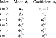
The energy analysis as described in § 3 is performed for the constructed global modes and the mean flow. Note that since the time-averaged and the constructed fluctuating coherent velocity fields are now available over the entire observation volume, the spatial derivatives can be calculated directly. Here, a second-order centred scheme was used to calculate the gradients. As summarized in table 3, the mean flow is denoted by index
 $i=0$
, and
 $i=1,2$
refer to antisymmetric (first) harmonic pair,
 $i=3,4$
to symmetric (second) harmonic pair, and
 $i={\it\Delta}$
to the slow-drift mode.
Indices used to denote the constructed global modes considered in the energy analysis.
4.2 Total energy flow
The energy terms in (3.13) and (3.14) are shown in figure 16. Each of the three terms
 $C_{0}$
,
 $T_{0}$
and
 $D_{0}$
in the mean base-flow energy equation are calculated from the measured data, and the pressure work
 $F_{0}$
is estimated from the residual. With the dissipation being negligible, the convected MKE into the domain is balanced by the mean pressure work and the energy interactions of the mean flow with turbulent fluctuations (loss to turbulence).
Energy terms in the modal and base-flow energy balance equations. Grey and white bars show positive and negative values, respectively. The estimated uncertainty for the individual terms is 0.008.

As is expected for a sufficiently large observation domain, the TKE transfer term
 $T$
is negligible. Consequently, the magnitude of the transfer from the mean to fluctuations
 $T_{0}$
in the MKE equations is almost equal to the production of turbulence
 $P$
in the TKE equation as implied by (3.15). Hence, in the MKE equation,
 $T_{0}$
acts as a sink, while in the TKE equation,
 $P$
is the only source term.
Approximately
 $28\,\%$
of the TKE production is convected from the domain, giving a residual of
 $72\,\%$
, which, neglecting the pressure work, provides an estimate for the transfer to the unresolved modes and dissipation to heat in the small-scale fluctuations. Generally, three-dimensionality has a mitigating effect on the role of the pressure term in the Galerkin model. By analogy to the 3D shear layer, the pressure work is expected to be two orders of magnitude smaller than the production or dissipation terms (Noack et al.
Reference Noack, Papas and Monkewitz2005). The dissipation term is significantly larger than the convection term. Consider that the observation domain encompasses the end of the formation region and the very near wake. When compared to the similar region of a 2D cylinder wake in a low-Reynolds-number transitional regime, similar observations are made (Noack Reference Noack2006).
In the cylinder study, the wake was subdivided into three observation domains: the first extending from the cylinder to 10 diameters downstream; the second from 10 to 20 diameters; and the third further downstream. In the first domain, where the shedding is described as 2D, with the shed vortices (rollers) undergoing little spanwise deformation, the production term exceeds the dissipation (losses to higher-order modes) by a factor of 2–3 times. The convection term is also observed to be significantly larger than the dissipation term. In the second domain, where the deformation of the roller vortices is increasingly significant, the magnitude of the production term is only slightly larger than that of the dissipation and, in comparison, the convection term is significantly smaller. Further downstream, production decreases further and convection is negligible.
Noack (Reference Noack2006) attributes the high dissipation rates of wake and mixing layers to increased three-dimensionality due to the effect of mode B rib structures deforming the relatively stronger shed roller vortices. In the present flow, this 3D effect is expected to be even more pronounced due to the interaction of the two coexisting and strong structures in the base and tip regions (see § 4.5). These structures arise in the immediate obstacle wake, suggesting that the 3D effects arise earlier. The present results are consistent with a more rapid evolution when compared to the relatively less complex cylinder wake. For the pyramid case, for which the observation domain extends from
 $0.8d$
to
 $2.3d$
, the relative contributions of the energy terms resemble those observed in the second domain of the cylinder case: the production is larger but comparable to the dissipation, while the convection term is significantly smaller.
4.3 Modal energy flows
The modal contributions of (3.16) are shown in figure 17. Approximately
 $60\,\%$
of the total production arises in the fundamental harmonic pair, and only
 $1.2\,\%$
in the second harmonics. Consistent with a forward energy cascade, the energy is transferred from the fundamental pair (negative) to the second harmonics (positive). The residual represents the transfer to the unresolved scales, i.e. higher-order modes (HOM), since the fluctuating pressure work can be considered small. The energy transfer of both the resolved harmonics is negative, suggesting a transfer from the large scales to smaller-scale turbulence. As is discussed below in considering the distribution of the Galerkin coefficient densities, the transfer to HOM can be linked to the shear layer (Noack et al.
Reference Noack, Papas and Monkewitz2005). The rather large transfer to HOM observed in this work emphasizes that the 3D shear layer has a stronger influence in exciting the higher harmonics, when compared to 2D wakes.
Time-averaged modal energy contributions and the residual inferred to approximate the unresolved transfer terms for the TKE balance of (3.16). The right-hand axis shows the magnitude as a percentage of the total mean production. The uncertainty for the individual terms is estimated to be 0.0015.

Figure 18 summarizes the average energy flow between the resolved scales (the slow-drift mode, fundamental and second harmonic pair), and all the other unresolved scales lumped into one term (HOM). This map includes the modal contributions of figure 17 as well as the production, convection and dissipation contributions of the unresolved scales, estimated from (3.14) by subtracting the contribution of the resolved scales. The unresolved terms gain
 $85.9\,\%$
from the mean and interactions with the fundamental and second harmonic pairs, from which
 $72.1\,\%$
is dissipated and the rest is convected. The dissipation, therefore, is an important energy mechanism in the considered measurement domain.
Considering only the time-averaged flow misleadingly ignores surprisingly important transient dynamics. The highest values and the standard deviations of these mean values are also shown in figure 18. The variations are quite large: the production of the fundamental pair can be up to
 $140\,\%$
of the mean total production, and the transfer to the HOM up to
 $110\,\%$
. While a forward energy cascade is observed in the mean, temporal variations show backscatter of TKE as well. More noticeable is the energy transfer of the slow-drift mode. While no significant contributions are indicated on average, this mode has an active role away from the limit cycle. Temporal variations show that the instantaneous energy transfer between this mode and the fundamental pair can be up to
 $\pm 30\,\%$
of the mean total production. Time averaging hides these large interactions. In the next section, closer consideration is given to the temporal variations of the transfer terms and couplings of the slow-drift mode with the fundamental harmonic pair.
The mean values of the energy flow (as percentages of the mean total production) and standard deviations with arrows indicating the average direction. The maximum and minimum values are presented in brackets
 $[\min ,\max ]$
, with negative values indicating reversal of the energy flows.

4.4 Temporal evolution of modal energy flows
The temporal variations of the energy transfers of the first harmonic pair with the slow-drift mode
 $T_{{\it\Delta}a}$
and the second harmonics
 $T_{sa}$
are shown in figure 19, together with the corresponding time traces for
 $a_{{\it\Delta}}$
and
 $a_{u}^{(1)}$
for reference. Note that no significant energy transfer is present between the slow-drift mode and the second harmonics, i.e.
 $T_{{\it\Delta}s}\equiv 0$
. The temporal variations of
 $T_{sa}$
show that the forward energy cascade is dominant, with few instances of low backscatter of energy.
Transfer of the fundamental harmonic pair (b) with the symmetric pair
 $T_{sa}$
(blue) and the slow-drift mode
 $T_{{\it\Delta}a}$
(red), with the modal coefficients (a). The highlighted intervals show examples of relatively low
 $a_{{\it\Delta}}$
, when delayed energy transfers to the second harmonics occur. The right-hand axis shows the magnitude as a percentage of the total mean production.

Another important observation is the energy flow sequence. At high-amplitude cycles with
 $a_{{\it\Delta}}>0$
, energy flows from the first harmonic pair, at the same time, to both the slow-drift mode and the second harmonic pair, i.e.
 $T_{{\it\Delta}a}>0$
,
 $T_{sa}>0$
. At low-amplitude cycles with
 $a_{{\it\Delta}}<0$
, energy flows from the slow-drift mode to the first harmonics and then with a delay transfers to the second harmonics, i.e.
 $T_{{\it\Delta}a}<0$
,
 $T_{sa}>0$
. Two examples of the latter are highlighted in figure 19. At the third highlighted interval, the energy of the first harmonic pair remains low for a long period and the energy flow to the second pair is almost zero.
The coupling and energy exchange between the slow-drift mode with the fundamental pair is consistent with the mean-field theory. Figure 20 shows two examples away from the limit cycle: (1) a cycle above the average cycle with an amplitude larger than the average, and (2) another below the average cycle with an amplitude smaller than the average. In case (1) the transfer from slow-drift mode to the antisymmetric pair is positive, whereas in case (2) the transfer is in the opposite direction. In both of these cases, the energy exchange drives the flow state towards the mean (oscillatory) solution. The distribution
 $a_{{\it\Delta}}$
versus
 $T_{{\it\Delta}a}$
, shown in figure 20(c), emphasizes that the direction of the energy transfer depends explicitly on the sign of
 $a_{{\it\Delta}}$
for all observed cycles.
The aforementioned dynamic behaviour may be interpreted as the response of a stable nonlinear oscillator to perturbations, where the average solution represents an attractor. As a heuristic example, if a shear layer feeding the forming vortices is perturbed, which corresponds to a base-flow fluctuation and deviation from
 $a_{{\it\Delta}}=0$
, the vorticity flux to the vortex is modified (i.e. the amplitude of the fundamental pair is altered), which in turn induces a change in the base flow, tending to restore the average cycle. The source of the perturbations results from the instantaneous effect of a combination of the other modes, that is, the background turbulence. This can be seen explicitly by considering the evolution equations for the individual modes, obtained simply by taking the inner product of the mode of interest and the Navier–Stokes equations (Couplet et al.
Reference Couplet, Sagaut and Basdevant2003). This operation results in the appearance of terms involving products of the temporal mode coefficients, analogous to the Reynolds-stress terms. While these terms must vanish identically under temporal averaging, these are instantaneously non-zero and act as source/sink terms. These Reynolds-stress-like terms form the contributions to the triadic interactions found in the transfer and production terms involving
 $q_{ijk}^{c}$
and
 $q_{ii0}^{c}$
, respectively. Thus, energy can be transferred directly and independently to the individual modes, as is represented in figure 18. The transfer term
 $T_{{\it\Delta}a}$
then acts to drive the solution towards the average cycle.
Direction of the energy transfer between the slow-drift mode and fundamental pair. (a) The
 $a_{u}^{(2)}$
versus
 $a_{u}^{(1)}$
phase portrait for two representative cycles, one above (red) and one below (blue) the average cycle (
 $a_{{\it\Delta}}=0$
, indicated in black). In both cases, the motion is clockwise. (b) Plot of
 $a_{{\it\Delta}}$
versus
 $a_{u}^{(1)}$
for all measurements (green dots) and the representative cycles of (a) with corresponding colours. The arrows indicate that the energy exchange drives the flow towards the average cycle. At high amplitudes of the fundamental,
 $a_{{\it\Delta}}>0$
,
 $T_{{\it\Delta}a}>0$
and energy flows to the slow-drift mode and the amplitude of the oscillations is dampened. Conversely, at low amplitudes,
 $a_{{\it\Delta}}<0$
,
 $T_{{\rm\Delta}a}<0$
and energy flows to the fundamental pair, tending to amplify the oscillation. (c) Plot of
 $a_{{\it\Delta}}$
versus
 $T_{{\it\Delta}a}$
showing that the direction of the energy flow depends explicitly on the sign of
 $a_{{\it\Delta}}$
.

4.5 Local distributions and link to physics
The results presented so far are the net global events summed over the whole spatial domain. The local distributions can provide more details about the interactions, and help to identify the links between energetic events and topological differences. As per (3.10),
 $\widetilde{q}_{ijk}^{c}$
denotes the convection Galerkin coefficient density to differentiate from the integral Galerkin coefficients
 $q_{ijk}^{c}$
.
For a clearer illustration of the local distributions in figures 21–24, the limits of the isosurfaces are selected objectively by taking the values that enclose a specific fraction of the modal contributions. Two limits are considered, the surface enclosing
 $95\,\%$
(transparent) of the contribution, and another enclosing
 $50\,\%$
(opaque) to identify localized areas of concentration. The blue/teal and yellow/red colours indicate negative and positive values, respectively.
The isosurfaces of the local Galerkin coefficient densities
 $\widetilde{q}_{0ii}^{c}$
are shown in figure 21. This term includes two contributions, loss to turbulence, which is equal and opposite to modal production, and transfer of mean kinetic energy by fluctuations. The contribution of the transport terms integrated over the spatial domain is zero, as discussed in § 4.2. This redistributed nature of the transfer terms can be deduced from figure 21. The positive contributions are concentrated on the low-speed side of the shear layer (i.e. inside the wake core, see figure 4 for reference). These are offset by the negative contributions at the wake boundaries on the high-speed side of the shear layers.
Isosurfaces of the Galerkin transfer modal coefficient densities
 $\widetilde{q}_{0ii}^{c}$
representing interactions of the mean flow with the (a) first and (b) second harmonic pairs. Transparent and opaque volumes, respectively, contain
 $95\,\%$
and
 $50\,\%$
of the summed contribution, with blue/teal and red/yellow showing negative and positive values, respectively. The displayed rectangle corresponds to the observation domain and has a similar orientation as in figure 10.

Same as figure 21 but for modal production coefficient densities
 $\widetilde{q}_{ii0}^{c}$
.

The distribution of the modal production coefficient densities
 $\widetilde{q}_{ii0}^{c}$
is shown in figure 22 for the fundamental and second harmonic pairs. As expected, these terms are positive (source) terms. The modal production coefficients of the fundamental pair, shown in figure 22(a), are extremely localized at regions close to the wall where the mean velocity gradients are high. Similar to the cylinder wake, the contribution from the shear layer is not large. On the other hand, for the second harmonics, the shear layer plays a significant role. As shown in figure 22(b) the high-production regions are closer to the boundaries of the wake. Moreover, they occur further downstream of the regions where the production of the fundamental pair is concentrated. These observations are consistent with the expected energy flow sequence from larger to smaller scales. The production of the largest scales is related to the vorticity flux at the solid boundaries, while the smaller scales arise from 3D vortex dynamics as occurring, for instance, in the shear layers.
Same as figure 21 but for modal convection coefficient densities
 $\widetilde{q}_{i0i}^{c}$
.

Same as figure 21 but for modal transfer coefficients,
 $\widetilde{q}_{{\rm\Delta}ii}^{c}$
, representing interactions of the slow-drift mode with the fundamental harmonic pair.

The differences between the distributions of the transfer
 $\widetilde{q}_{0ii}^{c}$
and production
 $\widetilde{q}_{ii0}^{c}$
terms highlight the different roles played by the fluctuating and mean field in the energy flow. As can be seen in table 1, the transfer terms contain the spatial gradients of the fluctuating components, while the production terms contain the mean velocity gradients.
The modal convection coefficients in figure 23 show regions of positive and negative values, as is expected from the periodic nature of the flow. Similar to the production terms, concentrated regions are observed close to the pyramid and the wall where gradients are high for the fundamental pair, and closer to the edge of the wake for the second harmonics.
The global couplings of the slow-drift mode and the fundamental pair were discussed in § 4.4. The transfer term as defined in § 3.3 includes 16 terms, from which only two terms have significant contributions. The modal coefficient densities for these two terms are shown in figure 24. The sign of both terms changes in the region close to the mean vortex pair at the tip. In the wake core region, both coefficients are positive (yellow coloured) and the local direction of the energy flow matches that observed with the global behaviour: energy is extracted by the slow-drift mode when
 $a_{{\it\Delta}}>0$
and is lost to the fundamental pair when
 $a_{{\it\Delta}}<0$
. The local energy flow in the tip region (blue coloured), however, is in the opposite direction.
The aforementioned local change in the energy flow direction can be related to the interaction between the base and tip region vortices. Consider the vortex topology at three characteristic snapshots, taken at the same shedding phase, with (i)
 $a_{{\it\Delta}}<0$
, (ii)
 $a_{{\it\Delta}}=0$
(the typical or average cycle) and (iii)
 $a_{{\it\Delta}}<0$
as shown in figure 25. Significant topological differences are observed. The vortex topology is characterized with two types of vortex structures. In case (i) the base vortex is stronger than the second vortex with a streamwise part in the tip region. Here, the energy transfer with the slow-drift mode tends to strengthen the tip region vortex and weaken the base vortex. In contrast, in case (ii) the second vortex with a streamwise part at the tip region is stronger and the energy flow is reversed. The transfer term
 $T_{{\it\Delta}a}$
for a point on the average cycle is negligible. It thus appears that the exchange between the slow-drift mode and the fundamental pair are physically expressed as interplay between these vortex structures about the average flow state.
Isosurfaces of
 ${\it\lambda}_{2}=-0.01$
representing the vortex structures at an instant of (a) negative, (b) zero and (c) positive slow-drift coefficients, coloured with transfer term
 $T_{{\it\Delta}a}$
.

5 Conclusions
A detailed modal energy analysis is presented for the 3D velocity modes of the highly modulated turbulent wake. The modes were constructed from planar PIV measurements and simultaneous wall pressure data using a sensor-based estimation technique that renders the main features of the wake and vortex topology (Hosseini et al. Reference Hosseini, Martinuzzi and Noack2015).
The oscillatory pyramid wake is found to have significantly different energy mechanisms as compared to the 2D cylinder wake. The excitation of the higher harmonics is stronger and the energy transfer plays an important role in damping the energy. The fundamental pair contributes to
 $60\,\%$
of the total production. Approximately
 $78\,\%$
of this contribution is transferred to higher harmonics, which eventually gets dissipated in small-scale turbulence. The dissipation, rather than convection (Noack et al.
Reference Noack, Papas and Monkewitz2005; Noack Reference Noack2006), is shown to be the dominant energy sink.
Even in the presence of such significant differences, strong couplings are observed between the slow-drift (non-oscillatory) mode and the fundamental (unstable) pair. Surprisingly, the transient dynamics are still described with such couplings that were originally derived for the vortex shedding instability at transitional Reynolds number
 $Re_{crit}=47$
.
The temporal variations indicate sequences of large energy transfers in the transitional states. Two characteristic events are generally observed: (i) in-phase energy transfer from the fundamental pair to the slow-drift mode and second harmonics at instances with
 $a_{{\it\Delta}}>0$
; and (ii) out-of-phase transfer from the slow-drift mode to the fundamental pair and subsequently to second harmonics at instances with
 $a_{{\it\Delta}}<0$
.
The spatial distributions of the temporally averaged energy terms indicate extremely localized concentrations of production and convection. While the fundamental pair is mainly created at regions close to the wall, the second harmonics are created at the wake boundaries close to the shear layer. Observing the topology of the shed vortices, the transfer dynamics in the shear layer appear to be linked to the interaction between two coexisting structures. This feature distinguishes the pyramid wake flow from that of the cantilevered finite cylinder flow, where only the Kármán-type structures are observed.
Looking forward, this work offers a different perspective for exploiting experimental data. The modal analysis results in an elegant and quantifiable description of coherent structure interactions in terms of energy flows and the path along the energy cascades towards small-scale motion. It highlights the significance of instantaneous exchanges, ultimately underlying the generation of Reynolds stresses, which are masked in the time-averaged terms. Further scrutiny provides localized details of vortex interaction phenomenology. Such insights are often critical guides in formulating flow control strategies as seen in Mills, Sheridan & Hourigan (Reference Mills, Sheridan and Hourigan2003). The remarkable link to mean-field theory motivates our work in developing dynamically consistent reduced-order models towards applications in flow control theory (Brunton & Noack Reference Brunton and Noack2015).
More generally, the present analysis potentially contributes to an original framework for comparing data from PIV and URANS simulations. On a kinematic level, the estimation technique can extract base-flow deformations and the oscillatory structures that a URANS simulation can be expected to predict. On a dynamic level, the energy flows between base flow, oscillatory structures and residual have been quantified from PIV data in the proposed analysis. Thus production, convection, dissipation and transfer terms of URANS simulations can be locally and globally compared with the inferred experimental data. Finally, further analysis of the residual field can form the basis for subsequent refinement of modelled terms. As alternative to URANS simulations, Liu has pioneered shear turbulence models with stability modes for the coherent structures and energy transfer models accounting for the stochastic fluctuations (Liu Reference Liu1989).
Acknowledgements
The authors acknowledge funding from the Natural Sciences and Engineering Research Council of Canada (NSERC) and the ANR Chair of Excellence TUCOROM (ANR-CEXC-2010-0015). The authors thank the anonymous reviewers for their insightful comments and suggestions, which have contributed to strengthening this paper.
Appendix. Estimation technique
As a starting point, the salient features of EPOD (Borée Reference Borée2003) are reiterated for continuity. First, the spatio-temporal pressure data acquired at locations
 $\boldsymbol{y}$
from
 $N_{p}$
sensors are expanded onto the POD basis:
 $p(\boldsymbol{y},t)=\sum _{n=1}^{N_{p}}a_{p}^{(n)}(t){\it\phi}_{p}^{(n)}(\boldsymbol{y})$
, where
 $a_{p}^{(n)}(t)$
and
 ${\it\phi}_{p}^{(n)}(\boldsymbol{y})$
denote the
 $n$
th temporal coefficient and spatial modes, respectively. The extended velocity modes are then defined,
 ${\bf\psi}_{u}^{(n)}(\boldsymbol{x})=\langle a_{p}^{(n)}(t)\boldsymbol{u}(\boldsymbol{x},t)\rangle /{\it\lambda}_{p}^{(n)}$
, where
 $\langle \cdot \rangle$
denotes the time-averaging operator,
 ${\it\lambda}_{p}^{(n)}=\langle a_{p}^{(n)}(t)a_{p}^{(n)}(t)\rangle$
and
 $\boldsymbol{x}$
denotes the velocity spatial domain. The velocity, then, is estimated using
 $$\begin{eqnarray}\displaystyle \hat{\boldsymbol{u}}(\boldsymbol{x},t_{est})=\mathop{\sum }_{n=1}^{N_{mode}}a_{p}^{(n)}(t_{est}){\bf\psi}_{u}^{(n)}(\boldsymbol{x}), & & \displaystyle\end{eqnarray}$$
where
 $t_{est}$
denotes the estimation time and
 $N_{mode}\leqslant N_{p}$
. If all extended modes are used (i.e.
 $N_{mode}=N_{p}$
) the linear stochastic estimation technique is recovered. To render a consistent flow topology and the transient dynamics, the EPOD technique is modified in four respects:
Expansion onto the optimal basis. The fluctuating velocity component is expanded onto a basis, which, by construction, is orthonormal following the procedure depicted in figure 26. Briefly, after subtraction of the time-averaged mean, the fluctuations are decomposed into symmetric and antisymmetric fields according to:
 $$\begin{eqnarray}\displaystyle \left.\begin{array}{@{}c@{}}u_{s}(x,y,z,t)=[u^{\prime }(x,y,z)+u^{\prime }(x,-y,z)]/2,\\ u_{a}(x,y,z,t)=[u^{\prime }(x,y,z)-u^{\prime }(x,-y,z)]/2,\\ v_{s}(x,y,z,t)=[v^{\prime }(x,y,z)-v^{\prime }(x,-y,z)]/2,\\ v_{a}(x,y,z,t)=[v^{\prime }(x,y,z)+v^{\prime }(x,-y,z)]/2,\\ w_{s}(x,y,z,t)=[w^{\prime }(x,y,z)+w^{\prime }(x,-y,z)]/2,\\ w_{a}(x,y,z,t)=[w^{\prime }(x,y,z)-w^{\prime }(x,-y,z)]/2.\end{array}\right\} & & \displaystyle\end{eqnarray}$$
This decomposition confers beneficial convergence behaviour for the spatial modes (Holmes et al. Reference Holmes, Lumley, Berkooz and Rowley2012), which is paramount to the accuracy of the estimation. The benefits have been verified to outweigh the potential risk due to cross-talk arising from experimental uncertainty.
Algorithm used to obtain the orthonormal subspace onto which the velocity data are expanded.

The antisymmetric harmonic modes are determined from a POD of the antisymmetric field. The symmetric field is decomposed into a slowly varying part using the Gaussian short-time averaging operator and a fast varying part. The most energetic mode of the slowly varying part is taken to represent the low-frequency base-flow variations (slow-drift mode) and the symmetric harmonic modes are obtained from the POD of the fast varying part.
The five most energetic modes in plane
 $z/h=0.23$
are shown in figure 27. The two most energetic modes compose the fundamental antisymmetric pair with frequency
 $f_{c}$
, the shedding frequency. The third most energetic mode is the slow-drift mode following with the symmetric harmonic pair with frequency
 $2f_{c}$
. The combination of these five modes contributes to
 $60.8\,\%$
of the total TKE of this plane.
(a) Contours of velocity spatial modes at the plane
 $z/h=0.23$
. The dashed lines indicate negative values. Subscripts
 $a$
,
 $s$
and
 ${\it\Delta}$
indicate the antisymmetric, symmetric and slow-drift modes, respectively. (b) The PSDFs of the corresponding temporal coefficients. Spectra are in log–log scale and offset for clarity.

By expanding the velocity data onto the orthonormal basis as in (A 3), the correlations between the spatio-temporal velocity data and the pressure coefficients of
 ${\bf\psi}_{u}^{(n)}$
reduce to correlations between the temporal coefficients as per (A 4):
 $$\begin{eqnarray}\displaystyle & \displaystyle \hat{\boldsymbol{u}}(\boldsymbol{x},t_{est})=\mathop{\sum }_{k=1}^{N_{u}}\hat{a}_{u}^{(k)}(t_{est}){\bf\phi}_{u}^{(k)}(\boldsymbol{x}), & \displaystyle\end{eqnarray}$$
 $$\begin{eqnarray}\displaystyle & \displaystyle \hat{a}_{u}^{(k)}(t_{est})=\mathop{\sum }_{n=1}^{N_{mode}}a_{p}^{(n)}(t_{est})\frac{\langle a_{p}^{(n)}(t)a_{u}^{(k)}(t)\rangle }{{\it\lambda}_{p}^{(n)}}, & \displaystyle\end{eqnarray}$$
 ${\bf\phi}_{u}^{(k)}(\boldsymbol{x})$
and
 $a_{u}^{(k)}(t)$
are, respectively, velocity basis modes and corresponding temporal coefficients. This simplification significantly reduces the computational effort and makes it possible to explicitly detect and extract the existing correlations in given data. Only the pressure modes for which the correlation with the velocity field is non-vanishing are used in the estimation. Hence, this approach eliminates the need for additional ranking criteria for selection and reduces the experimental uncertainty introduced by including non-contributing modes (cf. Sicot et al.
Reference Sicot, Perrin, Tran and Borée2012; Clark, Naghib-Lahouti & Lavoie Reference Clark, Naghib-Lahouti and Lavoie2014). Here, when considering only the non-vanishing correlations, the estimation of the velocity coefficients for the first harmonic pair (
 $k=1,2$
) and the slow-drift (
 ${\it\Delta}$
) reduce to
 $$\begin{eqnarray}\displaystyle \left.\begin{array}{@{}c@{}}\displaystyle \hat{a}_{u}^{(k)}(t_{est})=a_{p}^{(1)}(t_{est})\frac{\langle a_{p}^{(1)}(t)a_{u}^{(k)}(t)\rangle }{{\it\lambda}_{p}^{(1)}}+a_{p}^{(2)}(t_{est})\frac{\langle a_{p}^{(2)}(t)a_{u}^{(k)}(t)\rangle }{{\it\lambda}_{p}^{(2)}},\\ \displaystyle \hat{a}_{{\it\Delta}}(t_{est})=a_{p}^{G}(t_{est})\frac{\langle a_{p}^{G}(t)a_{{\it\Delta}}(t)\rangle }{{\it\lambda}_{p}^{G}},\end{array}\right\} & & \displaystyle\end{eqnarray}$$
where
 $a_{p}^{(1)}$
and
 $a_{p}^{(2)}$
are the antisymmetric pair coefficients, and
 $a_{p}^{G}$
is the slowly varying coefficient of the pressure data, found from a similar decomposition to that used for the
 $u$
component of the velocity field.
Sensor history for harmonic mode estimation. The multi-time-delay approach improves the estimation by forcing the convergence of the pressure harmonic modes (Lasagna, Orazi & Iuso Reference Lasagna, Orazi and Iuso2013) and accounting for the phase shift between the pressure and velocity harmonic coefficients (Durgesh & Naughton Reference Durgesh and Naughton2010). Briefly, the spatial information of the sensor data is obtained by treating the time-delayed signal as originating from a virtual sensor located downstream of the physical sensor. For
 $N$
physical sensors, and
 $M$
time-delayed signals, the POD is performed for a system of
 $N_{p}=N\times (M+1)$
sensors. The selection of time-delay interval
 ${\it\tau}_{T}$
and number of delayed signals
 $M$
is shown to affect the accuracy of the estimation (Durgesh & Naughton Reference Durgesh and Naughton2010; Sicot et al.
Reference Sicot, Perrin, Tran and Borée2012; Clark et al.
Reference Clark, Naghib-Lahouti and Lavoie2014; Hosseini et al.
Reference Hosseini, Martinuzzi and Noack2015). Following Hosseini et al. (Reference Hosseini, Martinuzzi and Noack2015), a time-delay interval of
 ${\it\tau}_{T}\approx 1/f_{c}$
and
 $M=10$
time-delayed signals are used to ensure that the first and second pressure harmonics follow the expected cyclical behaviour. The error of the estimation does not change significantly by addition of further delayed signals.
Fixing the phase of the slow-drift mode. The estimation of the velocity field is improved by including a time delay for the non-harmonic modes separately. Omitting this step introduces an artificial and random phase lag between the non-harmonic and harmonic fluctuations, resulting in a misrepresentation of the coherent strain field and the dynamics of the coherent motion. For the slow-drift mode, the time delay
 ${\it\tau}_{{\it\Delta}}$
is found from the peak of the cross-correlation function of the pressure,
 $a_{p}^{G}$
, and the velocity,
 $a_{{\it\Delta}}$
, coefficients. The correct phase in the estimation
 $\hat{a}_{{\it\Delta}}$
is recovered as shown in (A 6):
 $$\begin{eqnarray}\displaystyle \hat{a}_{{\it\Delta}}(t_{est})=a_{p}^{G}(t_{est}-{\it\tau}_{{\it\Delta}})\frac{\langle a_{p}^{G}(t-{\it\tau}_{{\it\Delta}})a_{{\it\Delta}}(t)\rangle }{{\it\lambda}_{p}^{G}}. & & \displaystyle\end{eqnarray}$$
Estimation of higher harmonics. The onset of vortex shedding in the bluff-body wake is of a Hopf bifurcation type and consists of a single pair of unstable eigenmodes with a positive growth rate and a range of stable modes that are highly damped. The system is approximated with an invariant manifold model (Noack et al. Reference Noack, Afanasiev, Morzyński, Tadmor and Thiele2003), where the active coordinates are aligned with the unstable modes and the stable modes are slaved to the active modes. Consistent with this model, it was shown in Hosseini et al. (Reference Hosseini, Martinuzzi and Noack2015) that a better estimation is obtained using a quadratic invariant-manifold approximation as in (A 7):
 $$\begin{eqnarray}\displaystyle \hat{a}_{u}^{(k)}=h_{k11}a_{p}^{(1)}a_{p}^{(1)}+h_{k22}a_{p}^{(2)}a_{p}^{(2)}+h_{k12}a_{p}^{(1)}a_{p}^{(2)}+\ell _{k3}a_{p}^{(3)}+\ell _{k4}a_{p}^{(4)}, & & \displaystyle\end{eqnarray}$$
where
 $k=3,4$
denote the second harmonic modes and
 $h_{kij}$
,
 $\ell _{ki}$
are the correlation coefficients. As shown in figures 11 and 14 of Hosseini et al. (Reference Hosseini, Martinuzzi and Noack2015), inclusion of the quadratic terms results in an increase of up to 300 % of the energy represented in the estimated second harmonic modes and improves the estimation of the streamline topology and the region covered by the vortex cores, when compared to the measured flow field.
Normally, the velocity field is well approximated with a linear mapping from pressure sensors. However, the mode coefficients associated with the second harmonics of the velocity field were shown to be much more accurately estimated as a quadratic function of the first harmonics of the pressure signal as compared to a linear relation with the second sensor harmonics. The phase and amplitude relation between first and second harmonics of the flow is thus exploited while the second sensor harmonics with low signal-to-noise ratio can be avoided. The Volterra series enables an elegant alternative estimation approach for broadband dynamics without simplifications based on harmonically related components (Baars & Tinney Reference Baars and Tinney2014).



