1 Introduction
Many physiological media exhibit non-Newtonian properties and are frequently viscoelastic due to the presence of high-molecular-weight long-chain solutes. Mammalian sperm cells migrate through the female reproductive tract, traversing highly viscoelastic liquids such as cervix mucus and cumulus cell matrix surrounding the egg (Suarez & Pacey Reference Suarez and Pacey2006; Okabe Reference Okabe2013). Similarly numerous bacteria and other infectious micro-organisms are capable of penetrating the viscoelastic mucosal barrier protecting many epithelia in the body (Ribet & Cossart Reference Ribet and Cossart2015), particularly the 30–
 $40~\text{m}^{2}$
of the human intestinal tract (Helander & Fandriks Reference Helander and Fandriks2014). More generally, the ubiquity of rheological fluids in biology and physiology, together with the need for cells to move through these, has extensively motivated the study of microswimmers in a viscoelastic medium.
In modelling the impact of the viscoelasticity of physiological media on microswimming, a variety of constitutive relations have been considered with diverse microswimmers, as comprehensively detailed by Spagnolie (Reference Spagnolie2015). For instance, one of the earliest classical studies was by Chaudhury (Reference Chaudhury1979), who considered an infinite two-dimensional swimming sheet – the eponymous Taylor sheet – within a second-order fluid model. An important step enabling simple, if approximate, modelling progress for analysing the motility of flagellates such as sperm was the extension of resistive force theory to linear viscoelasticity by Fulford, Katz & Powell (Reference Fulford, Katz and Powell1998). More recently, the explosion of interest in the theory of microswimming has led to numerous theoretical studies concerning the impact of viscoelasticity, particularly for flagellates and active filaments (Fu, Powers & Wolgemuth Reference Fu, Powers and Wolgemuth2007; Fu, Wolgemuth & Powers Reference Fu, Wolgemuth and Powers2008; Teran, Fauci & Shelley Reference Teran, Fauci and Shelley2010), as well as the motility of spherical squirmers (Zhu, Lauga & Brandt Reference Zhu, Lauga and Brandt2012; Yazdi, Ardekani & Borhan Reference Yazdi, Ardekani and Borhan2014, Reference Yazdi, Ardekani and Borhan2015; Corato, Greco & Maffettone Reference Corato, Greco and Maffettone2015). This has also been accompanied by numerous theoretical studies (e.g. Boehme & Mueller Reference Boehme and Mueller2015; Krieger, Spagnolie & Powers Reference Krieger, Spagnolie and Powers2015; Riley & Lauga Reference Riley and Lauga2015; Elfring & Goyal Reference Elfring and Goyal2016), numerical investigations (e.g. Thomases & Guy Reference Thomases and Guy2014; Salazar, Roma & Ceniceros Reference Salazar, Roma and Ceniceros2016) and experimental explorations (e.g. Godinez et al. Reference Godinez, Koens, Montenegro-Johnson, Zenit and Lauga2015; Gagnon & Arratia Reference Gagnon and Arratia2016; Gomez et al. Reference Gomez, Godinez, Lauga and Zenit2016), together with a recent extensive review (Patteson, Gopinath & Arratia Reference Patteson, Gopinath and Arratia2016) and research monograph (Spagnolie Reference Spagnolie2015), where further details on this fascinating subject may be found. However, a substantive difficulty is that there appears to be no characteristic response of inertialess swimmers to non-Newtonian rheologies, with differing observations on a case-by-case basis (Curtis & Gaffney Reference Curtis and Gaffney2013; Thomases & Guy Reference Thomases and Guy2014; Godinez et al. Reference Godinez, Koens, Montenegro-Johnson, Zenit and Lauga2015), especially for nonlinear media.
Given such complexity, there is merit in studying the simplest viscoelastic non-Newtonian constitutive relationship, namely linear viscoelasticity. Furthermore, the behaviour of particles and swimmers in such media is experimentally accessible. For particles this is illustrated by studies of micrometre-scale linear viscoelasticity (Gomez-Solano & Bechinger Reference Gomez-Solano and Bechinger2015), while a linear Maxwell model is observed to be a good approximation for the dilute methylcellulose solutions used as mucous analogues in studies of sperm motility (Smith et al. Reference Smith, Gaffney, Gadêlha, Kapur and Kirkman-Brown2009b ). Nonetheless, the linearly viscoelastic constitutive relation does not possess frame independence and hence it can only ever be an approximation (Spagnolie Reference Spagnolie2015). However, such corrections are degree two or higher in the fluid velocity and thus at sufficiently low velocity scales they are subdominant and can be consistently neglected at leading orders (Lauga Reference Lauga2014).
In addition, treating the swimmer deformation amplitude as sufficiently small also entails that the study of motility for a deforming body within a general non-Newtonian viscoelastic medium can, at leading order, be reduced to the study of swimming in a linearly viscoelastic medium (Lauga Reference Lauga2009, Reference Lauga2014). Importantly, given small deformations, the swimmer velocities and thus the swimmer dynamics are identical to those obtained for Newtonian Stokes flow, as first highlighted with resistive force theory and thus slender bodies by Fulford et al. (Reference Fulford, Katz and Powell1998) and more generally demonstrated for an arbitrary swimmer shape with an infinitesimally small deformation by Lauga (Reference Lauga2014).
Thus Purcell’s scallop theorem (Purcell Reference Purcell1977), which states that a microswimmer within a Newtonian Stokes medium cannot generate net locomotion by a reciprocal deformation (Ishimoto & Yamada Reference Ishimoto and Yamada2012), holds for small-deformation inertialess swimming in linear viscoelastic media. However, it is unclear whether this generalises to finite-amplitude swimming, not least due to the correspondence between inertialess linear viscoelastic flows on the one hand and unsteady Stokes flow on the other (Xu, Forest & Klapper Reference Xu, Forest and Klapper2007; Feng et al. Reference Feng, Cordoba, Hernandez, Indei, Li, Li and Schieber2016), noting that Purcell’s theorem does not hold for the latter. Hence one of our objectives below will be the consideration of Purcell’s theorem for finite-deformation swimming in a linear Maxwell fluid.
More fundamentally, our aims will concern the numerical simulation of microswimmer dynamics in linear viscoelastic media. Microswimmer computations have had a long tradition, with the initial seminal paper of Gray & Hancock (Reference Gray and Hancock1955) developing resistive force theory to enable the computation of approximate microswimming speeds by active slender bodies such as sperm. Since this time, many numerical methods have also been developed, and the boundary element method has emerged as a popular framework for computational simulation, enabling highly accurate prediction for swimmer dynamics in inertialess Newtonian flows with relatively small computational cost (Pozrikidis Reference Pozrikidis1992). This framework has also been applied in the solution of viscoelastic flows, treating the viscoelastic contribution to the stress tensor as a body force, necessitating either integration or the solution of elliptic partial differential equations over the three-dimensional flow domain. Hence a major advantage of the boundary element method formalism is lost, namely the ability to reduce to the system to integral equations over surfaces, thus avoiding the numerical meshing over the whole flow field (Phan-Thien, Tran-cong & Ramia Reference Phan-Thien, Tran-cong and Ramia1987; Zheng & Phan-Thien Reference Zheng and Phan-Thien1992; Phan-Thien & Fan Reference Phan-Thien and Fan2002).
In contrast, here, our prime objective is to construct an essentially standard boundary element framework, but with the novelty that this can be used to predict linearly viscoelastic inertialess swimmer dynamics, without recourse to considering the domain of the whole flow field, by using an analogy between the solutions for Newtonian Stokes flow and linear viscoelastic flow. While a more general linear viscoelastic boundary element method is developed in appendix A, in the main text we focus on the boundary element method for a linear Maxwell fluid, which also provides a generalisation of Purcell’s theorem for inertialess finite-deformation swimmers within linear Maxwell fluids.
We subsequently examine the dynamics of swimmers near boundaries, for the finite-deformation swimming of a tangential squirmer, a monotrichous (singly flagellated) bacterium and a mammalian sperm. In particular we examine the impact of linear Maxwell viscoelasticity and generalising previous works to assess whether it influences the mechanics of microswimmer boundary scattering and boundary accumulation, with the latter referring to the tendency of flagellated microswimmers to swim adjacent to surfaces.
Such studies are important in numerous contexts as exemplified by Pedley & Kessler (Reference Pedley and Kessler1992) emphasising the importance of preferential surface swimming for sperm to the fluid dynamics community. Subsequent studies on this topic have for instance greatly influenced our understanding of sperm guidance cues, such as whether surfaces are required for mammalian sperm rheotaxis, a candidate for long-range sperm navigation in the female reproductive tract (Miki & Clapham Reference Miki and Clapham2013; Ishimoto & Gaffney Reference Ishimoto and Gaffney2015; Zhang et al. Reference Zhang, Liu, Meriano, Ru, Xie, Luo and Sun2016). Further applications concern understanding and predicting sperm behaviours at the surface of the egg (Ishimoto, Cosson & Gaffney Reference Ishimoto, Cosson and Gaffney2016; Ishimoto & Gaffney Reference Ishimoto and Gaffney2016) and in microengineered devices (Denissenko et al. Reference Denissenko, Kantsler, Smith and Kirkman-Brown2012; Kantsler, Dunkel & Goldstein Reference Kantsler, Dunkel and Goldstein2013; Nosrati et al. Reference Nosrati, Driouchi, Yip and Sinton2015), which have many prospective applications from sperm sorting to precision in vitro fertilisation devices. The influence of bacterial motility near surfaces for biofilm initiation was first reported at least 20 years ago (Frymier & Ford Reference Frymier and Ford1997). Furthermore, given the importance of biofilm formation across society, for instance with over one million annual hospital acquired infections via medical devices in the USA (Bryers Reference Bryers2008), there is a major impetus to understanding bacterial motility on the approach to surfaces and whether surface design can reduce colonisation (Shum et al. Reference Shum, Tripathi, Yeomans and Balazs2013). As a final exemplar, we will use boundary elements to briefly consider the motion of a magnetically driven microswimmer, once more generalising to consider a linear viscoelastic fluid, noting that such devices are under intensive development, due to their potential in novel targeted drug delivery and medical diagnostic systems (Fusco et al. Reference Fusco, Ullrich, Pokki, Chatzipirpiridis, Ozkale, Sivaraman, Ergeneman, Pane and Nelson2014; Qiu et al. Reference Qiu, Lee, Mark, Morozov, Münster, Mierka, Turek, Leshansky and Fischer2014; Qiu & Nelson Reference Qiu and Nelson2015; Kim et al. Reference Kim, Lee, Lee, Nelson, Zhang and Choi2016).
All these examples are physiological and biological in nature since numerous biological fluids, and also their mimics in experimental settings, are viscoelastic. Thus the impact of viscoelasticity on motility in such circumstances is particularly relevant and linear viscoelasticity is the simplest extension from Newtonian media, well suited to dilute long-chain molecule solutions, as verified with dilute methylcellulose for instance (Smith et al. Reference Smith, Gaffney, Gadêlha, Kapur and Kirkman-Brown2009b ). All such investigations are contingent on external forces and torques, due either to magnetic fields or to boundary–swimmer interactions (Frymier et al. Reference Frymier, Ford, Berg and Cummings1995; Klein, Clapp & Dickinson Reference Klein, Clapp and Dickinson2003), and hence allow us to additionally highlight that external forces and torques must be handled differently in the linear viscoelastic framework developed below compared to the standard Newtonian boundary element method.
2 Problem settings
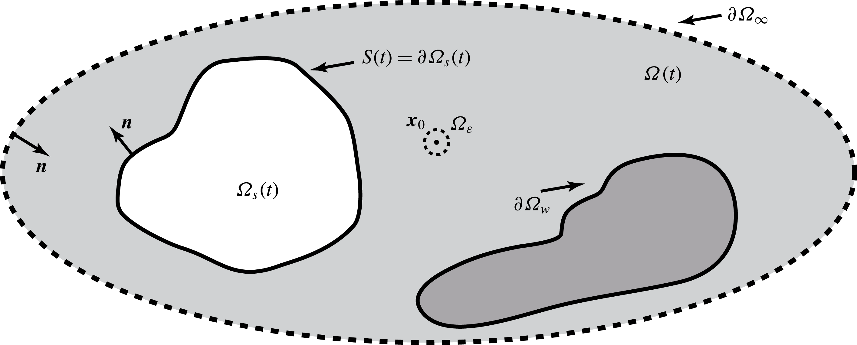
The regions external and internal to the swimmer are respectively denoted by
 $\unicode[STIX]{x1D6FA}(t)$
and
 $\unicode[STIX]{x1D6FA}_{s}(t)$
, and both are functions of time
 $t$
and depicted in the schematic of figure 1. The boundary of the internal region is
 $S=\unicode[STIX]{x2202}\unicode[STIX]{x1D6FA}_{s}$
and the boundary of the fluid region
 $\unicode[STIX]{x2202}\unicode[STIX]{x1D6FA}(t)$
is given by the union of
 $S$
, the time-independent wall boundary
 $\unicode[STIX]{x2202}\unicode[STIX]{x1D6FA}_{w}$
and the far boundary at spatial infinity
 $\unicode[STIX]{x2202}\unicode[STIX]{x1D6FA}_{\infty }$
, i.e.
 $\unicode[STIX]{x2202}\unicode[STIX]{x1D6FA}=\unicode[STIX]{x2202}\unicode[STIX]{x1D6FA}_{s}\cup \unicode[STIX]{x2202}\unicode[STIX]{x1D6FA}_{w}\cup \unicode[STIX]{x2202}\unicode[STIX]{x1D6FA}_{\infty }$
.
A schematic of the regions and boundaries of the system, as detailed in the text.

Around a microswimmer, the flow is effectively inertialess and characterised by a negligible Reynolds number, with the momentum balance given by
 $$\begin{eqnarray}\unicode[STIX]{x1D735}\boldsymbol{\cdot }\unicode[STIX]{x1D748}=0,\end{eqnarray}$$
where the stress tensor is defined as
 $\unicode[STIX]{x1D70E}_{ij}=-p\unicode[STIX]{x1D6FF}_{ij}+\unicode[STIX]{x1D70F}_{ij}$
(
 $i,j=1,2,3$
) for a pressure field
 $p$
and a deviatoric stress tensor
 $\unicode[STIX]{x1D749}$
. In a Newtonian fluid, i.e. Stokes flow, one has
 $\unicode[STIX]{x1D749}=2\unicode[STIX]{x1D707}\boldsymbol{D}$
, where
 $$\begin{eqnarray}D_{ij}=\frac{1}{2}\left(\frac{\unicode[STIX]{x2202}u_{i}}{\unicode[STIX]{x2202}x_{j}}+\frac{\unicode[STIX]{x2202}u_{i}}{\unicode[STIX]{x2202}x_{i}}\right)\end{eqnarray}$$
is the rate-of-strain tensor,
 $\unicode[STIX]{x1D707}$
is the constant viscosity of the fluid and
 $\boldsymbol{u}$
is the flow velocity, which also satisfies the incompressibility condition,
 $\unicode[STIX]{x1D735}\boldsymbol{\cdot }\boldsymbol{u}=0$
.
We impose no-slip boundary conditions on the wall and the swimmer surface. The equations of motion for the swimmer, with negligible inertia, reduce to the constraint that the swimmer experiences no net force or torque in the absence of external forcing.
In this paper, we generalise to consider a linear viscoelastic medium, focusing on a Maxwell fluid in the main text, where the deviatoric stress tensor satisfies the constitutive relation
 $$\begin{eqnarray}{\mathcal{L}}\unicode[STIX]{x1D749}:=\unicode[STIX]{x1D706}\frac{\unicode[STIX]{x2202}\unicode[STIX]{x1D749}}{\unicode[STIX]{x2202}t}+\unicode[STIX]{x1D749}=2\unicode[STIX]{x1D707}\boldsymbol{D},\end{eqnarray}$$
which approximates the flow properties of media such as dilute methylcellulose solutions (Smith et al.
Reference Smith, Gaffney, Gadêlha, Kapur and Kirkman-Brown2009b
), with
 $\unicode[STIX]{x1D706}$
the elastic relaxation time. In appendix A, we also consider a more general linear viscoelastic constitutive relation,
 $$\begin{eqnarray}{\mathcal{L}}\unicode[STIX]{x1D749}=2\unicode[STIX]{x1D707}{\mathcal{M}}\boldsymbol{D}:=2\unicode[STIX]{x1D707}\boldsymbol{D}+2\unicode[STIX]{x1D707}\unicode[STIX]{x1D6FE}\frac{\unicode[STIX]{x2202}\boldsymbol{D}}{\unicode[STIX]{x2202}t},\end{eqnarray}$$
where
 $\unicode[STIX]{x1D6FE}$
is a further response time scale.
The surface velocity of the swimmer
 $\boldsymbol{u}(\boldsymbol{x})$
is the combination of the linear, angular and shape deformation velocities,
 $\boldsymbol{U}+\unicode[STIX]{x1D734}\times \boldsymbol{x}+\boldsymbol{v}$
. We consider a swimmer with a prescribed shape deformation, and a swimmer forced by an external magnetic field, in both cases examining the resulting prediction of the linear and angular velocities
 $\boldsymbol{U}$
and
 $\unicode[STIX]{x1D734}$
. To proceed, we introduce two coordinate systems: the inertial reference frame with orthonormal Cartesian basis vectors
 $\{\boldsymbol{e}_{i}\}$
and the body-fixed frame with orthonormal basis vectors
 $\{\hat{\boldsymbol{e}}_{i}\}$
,
 $i\in \{1,2,3\}$
. The rotation from the body-fixed frame to the inertial reference coordinate frame is given by the matrix
 $\unicode[STIX]{x1D609}_{ij}=\boldsymbol{e}_{i}\boldsymbol{\cdot }\hat{\boldsymbol{e}}_{j}$
, and thus the deformation velocity in the reference frame is expressed by
 $v_{i}=\unicode[STIX]{x1D609}_{ij}(\text{d}\hat{x}_{j}/\text{d}t)$
, where
 $\text{d}\hat{x}_{j}/\text{d}t$
is a deformation velocity in the body-fixed frame and prescribed.
3 Boundary integrals
3.1 Reciprocal relations
The boundary integrals associated with the boundary element method are constructed via the reciprocal relation, which imposes a constraint on two sets of solutions
 $(\boldsymbol{u},\unicode[STIX]{x1D748})$
and
 $(\boldsymbol{u}^{\prime },\unicode[STIX]{x1D748}^{\prime })$
for the fluid equations within the same domain but with different boundary conditions. For Stokes flow, the reciprocal relation is (Pozrikidis Reference Pozrikidis1992)
 $$\begin{eqnarray}\frac{\unicode[STIX]{x2202}}{\unicode[STIX]{x2202}x_{j}}(u_{i}^{\prime }\unicode[STIX]{x1D70E}_{ij}-u_{i}\unicode[STIX]{x1D70E}_{ij}^{\prime })=0,\end{eqnarray}$$
with
 $\unicode[STIX]{x1D749}=2\unicode[STIX]{x1D707}\boldsymbol{D}$
. However, this no longer holds for linear viscoelastic media such as the Maxwell fluid we are considering, where
 ${\mathcal{L}}\unicode[STIX]{x1D749}=2\unicode[STIX]{x1D707}\boldsymbol{D}$
.
With the latter deviatoric stress,
 ${\mathcal{L}}\unicode[STIX]{x1D749}=2\unicode[STIX]{x1D707}\boldsymbol{D}$
, we consider
 ${\mathcal{L}}\unicode[STIX]{x1D70E}_{ij}$
instead of
 $\unicode[STIX]{x1D70E}_{ij}$
, and derive a similar reciprocal relation for a linearly viscoelastic fluid, given below by (3.9). The derivation is directly analogous to that presented in Pozrikidis (Reference Pozrikidis1992) for Newtonian flows, where further details may be found. To proceed, first consider the identity
 $$\begin{eqnarray}u_{i}^{\prime }\frac{\unicode[STIX]{x2202}}{\unicode[STIX]{x2202}x_{j}}({\mathcal{L}}\unicode[STIX]{x1D70E}_{ij})=\frac{\unicode[STIX]{x2202}}{\unicode[STIX]{x2202}x_{j}}(u_{i}^{\prime }{\mathcal{L}}\unicode[STIX]{x1D70E}_{ij})-\frac{\unicode[STIX]{x2202}u_{i}^{\prime }}{\unicode[STIX]{x2202}x_{j}}{\mathcal{L}}\unicode[STIX]{x1D70E}_{ij}.\end{eqnarray}$$
Focusing on the second term of the right-hand side above, note that the pressure term in the stress tensor does not contribute due to fluid incompressibility, so that
 $$\begin{eqnarray}\frac{\unicode[STIX]{x2202}u_{i}^{\prime }}{\unicode[STIX]{x2202}x_{j}}{\mathcal{L}}\unicode[STIX]{x1D70E}_{ij}=-\frac{\unicode[STIX]{x2202}u_{i}^{\prime }}{\unicode[STIX]{x2202}x_{i}}{\mathcal{L}}p+\frac{\unicode[STIX]{x2202}u_{i}^{\prime }}{\unicode[STIX]{x2202}x_{j}}{\mathcal{L}}\unicode[STIX]{x1D70F}_{ij}=\frac{\unicode[STIX]{x2202}u_{i}^{\prime }}{\unicode[STIX]{x2202}x_{j}}{\mathcal{L}}\unicode[STIX]{x1D70F}_{ij}=2\unicode[STIX]{x1D707}\frac{\unicode[STIX]{x2202}u_{i}^{\prime }}{\unicode[STIX]{x2202}x_{j}}D_{ij},\end{eqnarray}$$
where the last equality holds from the constitutive relation (2.3).
Hence we have
 $$\begin{eqnarray}u_{i}^{\prime }\frac{\unicode[STIX]{x2202}}{\unicode[STIX]{x2202}x_{j}}({\mathcal{L}}\unicode[STIX]{x1D70E}_{ij})=\frac{\unicode[STIX]{x2202}}{\unicode[STIX]{x2202}x_{j}}(u_{i}^{\prime }{\mathcal{L}}\unicode[STIX]{x1D70E}_{ij})-2\unicode[STIX]{x1D707}\frac{\unicode[STIX]{x2202}u_{i}^{\prime }}{\unicode[STIX]{x2202}x_{j}}D_{ij}.\end{eqnarray}$$
By analogy, we have the symmetric relation
 $$\begin{eqnarray}u_{i}\frac{\unicode[STIX]{x2202}}{\unicode[STIX]{x2202}x_{j}}({\mathcal{L}}\unicode[STIX]{x1D70E}_{ij}^{\prime })=\frac{\unicode[STIX]{x2202}}{\unicode[STIX]{x2202}x_{j}}(u_{i}{\mathcal{L}}\unicode[STIX]{x1D70E}_{ij}^{\prime })-2\unicode[STIX]{x1D707}\frac{\unicode[STIX]{x2202}u_{i}}{\unicode[STIX]{x2202}x_{j}}D_{ij}^{\prime }.\end{eqnarray}$$
Here, noting the definition of
 $D_{ij}$
and relabelling by
 $i\rightarrow j$
and
 $j\rightarrow i$
, we have
 $$\begin{eqnarray}\frac{\unicode[STIX]{x2202}u_{i}^{\prime }}{\unicode[STIX]{x2202}x_{j}}D_{ij}=\frac{\unicode[STIX]{x2202}u_{i}}{\unicode[STIX]{x2202}x_{j}}D_{ij}^{\prime },\end{eqnarray}$$
yielding the relation
 $$\begin{eqnarray}u_{i}^{\prime }\frac{\unicode[STIX]{x2202}}{\unicode[STIX]{x2202}x_{j}}({\mathcal{L}}\unicode[STIX]{x1D70E}_{ij})-u_{i}\frac{\unicode[STIX]{x2202}}{\unicode[STIX]{x2202}x_{j}}({\mathcal{L}}\unicode[STIX]{x1D70E}_{ij}^{\prime })=\frac{\unicode[STIX]{x2202}}{\unicode[STIX]{x2202}x_{j}}(u_{i}^{\prime }{\mathcal{L}}\unicode[STIX]{x1D70E}_{ij}-u_{i}{\mathcal{L}}\unicode[STIX]{x1D70E}_{ij}^{\prime }).\end{eqnarray}$$
The left-hand side of this relation, however, vanishes from the momentum-balance equations as
 $$\begin{eqnarray}u_{i}^{\prime }\frac{\unicode[STIX]{x2202}}{\unicode[STIX]{x2202}x_{j}}({\mathcal{L}}\unicode[STIX]{x1D70E}_{ij})=u_{i}^{\prime }{\mathcal{L}}\frac{\unicode[STIX]{x2202}\unicode[STIX]{x1D70E}_{ij}}{\unicode[STIX]{x2202}x_{j}}=0.\end{eqnarray}$$
Hence we finally obtain the reciprocal relation for linearly viscoelastic flow,
 $$\begin{eqnarray}\frac{\unicode[STIX]{x2202}}{\unicode[STIX]{x2202}x_{j}}(u_{i}^{\prime }{\mathcal{L}}\unicode[STIX]{x1D70E}_{ij}-u_{i}{\mathcal{L}}\unicode[STIX]{x1D70E}_{ij}^{\prime })=0.\end{eqnarray}$$
As with the Newtonian case (Pozrikidis Reference Pozrikidis1992), this reciprocal relation provides the keystone for the boundary element numerical methods, as detailed below.
3.2 Viscoelastic Stokeslet
In this subsection, we consider a Stokeslet for the linear viscoelastic fluid
 $G_{ij}$
, which is the Green function of this linear system and thus the velocity field when a point force at
 $\boldsymbol{x}_{0}$
is applied, defined as
 ${\mathcal{L}}(\unicode[STIX]{x1D735}\boldsymbol{\cdot }\unicode[STIX]{x1D748}^{\prime })_{ij}=-\unicode[STIX]{x1D6FF}_{ij}\unicode[STIX]{x1D6FF}(\boldsymbol{x}-\boldsymbol{x}_{0})$
, or
 $$\begin{eqnarray}-\frac{\unicode[STIX]{x2202}}{\unicode[STIX]{x2202}x_{i}}{\mathcal{L}}P_{j}+2\unicode[STIX]{x1D707}\unicode[STIX]{x1D6FB}^{2}G_{ij}=-\unicode[STIX]{x1D6FF}_{ij}\unicode[STIX]{x1D6FF}(\boldsymbol{x}-\boldsymbol{x}_{0}),\end{eqnarray}$$
where
 $P_{j}$
is the associated pressure and the singularity location,
 $\boldsymbol{x}_{0}$
, in general may be a function of time. We can therefore express the Stokeslet for the linear viscoelastic fluid by the solutions for the Newtonian Stokes flow,
 $$\begin{eqnarray}G_{ij}=G_{ij}^{S}\quad \text{and}\quad {\mathcal{L}}P_{j}=P_{j}^{S},\end{eqnarray}$$
with the superscript
 $S$
referring to Stokes flow.
Let the constant vector
 $\boldsymbol{q}$
be a force strength, and introduce a set of solutions for the linear viscoelastic fluid flow,
 $$\begin{eqnarray}u_{i}^{\prime }=\frac{1}{8\unicode[STIX]{x03C0}\unicode[STIX]{x1D707}}G_{ij}(\boldsymbol{x},\boldsymbol{x}_{0})q_{j},\quad p^{\prime }=\frac{1}{8\unicode[STIX]{x03C0}}P_{j}q_{j},\quad \unicode[STIX]{x1D70E}_{ij}^{\prime }=\frac{1}{8\unicode[STIX]{x03C0}}T_{ijk}q_{k},\end{eqnarray}$$
whereby we have
 $$\begin{eqnarray}{\mathcal{L}}\unicode[STIX]{x1D70E}_{ij}^{\prime }=-({\mathcal{L}}P_{m})q_{m}\unicode[STIX]{x1D6FF}_{ij}+2\unicode[STIX]{x1D707}D_{ij}^{\prime }=-\frac{1}{8\unicode[STIX]{x03C0}}P_{m}^{S}q_{m}+\frac{1}{8\unicode[STIX]{x03C0}}\left(\frac{\unicode[STIX]{x2202}G_{ip}^{S}}{\unicode[STIX]{x2202}x_{j}}+\frac{\unicode[STIX]{x2202}G_{jp}^{S}}{\unicode[STIX]{x2202}x_{i}}\right)q_{p}.\end{eqnarray}$$
This is equivalent to
 $$\begin{eqnarray}{\mathcal{L}}\unicode[STIX]{x1D70E}_{ij}^{\prime }=\unicode[STIX]{x1D70E}_{ij}^{\prime S},\end{eqnarray}$$
where
 $\unicode[STIX]{x1D70E}_{ij}^{\prime S}$
is the stress tensor for the Newtonian Stokes flow, given by
 $\unicode[STIX]{x1D70E}_{ij}^{\prime S}=(1/8\unicode[STIX]{x03C0})T_{ijp}^{S}q_{p}$
. Thus (3.14) can be rephrased as
 $$\begin{eqnarray}{\mathcal{L}}T_{ijp}=T_{ijp}^{S}.\end{eqnarray}$$
In principle there is an undetermined freedom regarding the initial condition. We thus assume the flow is stationary at initial time,
 $t_{0}$
, and then in turn
 $\unicode[STIX]{x1D70E}_{ij}^{\prime }$
is uniquely specified as the operator
 ${\mathcal{L}}$
is linear.
More generally, note that, in developing a boundary element method, one is constructing the flow field from the linear superposition of singularity solutions (Pozrikidis Reference Pozrikidis1992), and the choice of singularity solutions is the same as choosing a basis for a representation of the velocity field. Thus here we are using Newtonian velocity singularities, since
 $G_{ij}=G_{ij}^{S}$
, but the associated singularity pressure and stress fields are now more complex, and given by
 ${\mathcal{L}}P_{j}=P_{j}^{S}$
,
 ${\mathcal{L}}T_{ijp}=T_{ijp}^{S}$
, to ensure the reciprocal theorem holds. The latter in turn enables the construction of the boundary element method to find the decomposition of the flow field into singularity solutions even with linear viscoelasticity. However, the pressure and stress fields do not enter the final formalism and thus the net influence of linear viscoelasticity only significantly arises in the force and torque balances for the swimmer, which are, at most, modified in a simple manner. In turn, this enables a rapid adaptation of standard boundary element codes to study swimming in linearly viscoelastic media, as we shall derive and detail below.
3.3 Boundary integral equations
Based on the relations derived above, we are in a position to formulate the viscoelastic boundary integral equations, starting with the reciprocal relation (3.9). Substitution of the velocity and the stress of the point force flow
 $(\boldsymbol{u}^{\prime },\unicode[STIX]{x1D748}^{\prime })$
, obtained in (3.11) and (3.15), into the reciprocal relation gives us the relation for the velocity and the stress of our swimmer problem
 $(\boldsymbol{u},\unicode[STIX]{x1D748})$
as
 $$\begin{eqnarray}\frac{\unicode[STIX]{x2202}}{\unicode[STIX]{x2202}x_{j}}\left(\frac{1}{8\unicode[STIX]{x03C0}\unicode[STIX]{x1D707}}G_{ip}^{S}q_{p}({\mathcal{L}}\unicode[STIX]{x1D70E}_{ij})-\frac{1}{8\unicode[STIX]{x03C0}}u_{i}T_{ijp}^{S}q_{p}\right)=0.\end{eqnarray}$$
This relation is integrated over the fluid region except for a small sphere of radius
 $\unicode[STIX]{x1D716}$
around the singular point
 $\boldsymbol{x}_{0}$
,
 $\unicode[STIX]{x1D6FA}\backslash \unicode[STIX]{x1D6FA}_{\unicode[STIX]{x1D716}}$
, as depicted in figure 1. Noting the zero-velocity constraint on the wall boundary and at infinity, we have
 $$\begin{eqnarray}\int _{S\cup \unicode[STIX]{x2202}\unicode[STIX]{x1D6FA}_{\unicode[STIX]{x1D716}}}(G_{ip}^{S}({\mathcal{L}}\unicode[STIX]{x1D70E}_{ij})-\unicode[STIX]{x1D707}u_{i}T_{ipj}^{S})\boldsymbol{n}_{j}\,\text{d}S=0,\end{eqnarray}$$
where the vector
 $\boldsymbol{n}_{j}$
denotes the outward normal of the surface region, as in figure 1. The time derivative implicit within the operator
 ${\mathcal{L}}$
on the swimmer surface
 $S$
should be clarified. We take a larger region that covers the surface
 $S$
, with separation
 $\unicode[STIX]{x1D6FF}>0$
from it, and consider the time derivatives for the variables outside
 $S$
but in the larger region, where the derivative is unambiguously defined, before taking the limit of
 $\unicode[STIX]{x1D6FF}\rightarrow 0$
.
Exactly as in the Newtonian case (Pozrikidis Reference Pozrikidis1992, p. 26), the integral over
 $\unicode[STIX]{x2202}\unicode[STIX]{x1D6FA}_{\unicode[STIX]{x1D716}}$
converges to
 $8\unicode[STIX]{x03C0}\unicode[STIX]{x1D707}u_{p}(\boldsymbol{x}_{0})$
in the limit of
 $\unicode[STIX]{x1D716}\rightarrow 0$
, yielding the viscoelastic boundary integral equation,
 $$\begin{eqnarray}u_{p}(\boldsymbol{x}_{0})=-\frac{1}{8\unicode[STIX]{x03C0}\unicode[STIX]{x1D707}}\int _{S}G_{ip}^{S}({\mathcal{L}}\unicode[STIX]{x1D70E}_{ij})\boldsymbol{n}_{j}\,\text{d}S+\frac{1}{8\unicode[STIX]{x03C0}}\int _{S}u_{i}T_{ipj}^{S}\boldsymbol{n}_{j}\,\text{d}S.\end{eqnarray}$$
The first of these integrals is known as a single-layer boundary integral, while the second is known as a double-layer boundary integral. The latter requires care in its treatment, as the integrand is singular, and not just weakly singular. The evaluation of these integrals in the Newtonian case is fully documented (e.g. Pozrikidis Reference Pozrikidis1992) and immediately generalises to (3.18), as the double-layer singularity,
 $T_{ijk}^{S}$
, is the Newtonian singularity. However, we do not follow this approach here. Instead we explicitly assume the swimmer volume is invariant. Then it is much simpler to eliminate the second integral of (3.18), and write
 $u_{p}(\boldsymbol{x}_{0})$
in terms of only a single-layer boundary integral, as is well known for the Newtonian boundary element method (Pozrikidis Reference Pozrikidis1992) and as we now demonstrate for linear viscoelasticity.
To proceed, let
 $^{\ast }$
denote variables associated with a fictitious virtual flow within the interior of the swimmer
 $\unicode[STIX]{x1D6FA}_{s}(t)$
on making the supposition that the swimmer interior is constituted from the same linear viscoelastic medium as external to the swimmer. For example, let
 $\boldsymbol{u}^{\ast }$
denote the velocity field of this internal swimmer flow; its incompressibility immediately requires the restriction that swimmer volume is invariant. Given this, the same reciprocal relation (3.9) then holds in the interior region
 $\unicode[STIX]{x1D6FA}_{s}$
, and integrating over this region yields
 $$\begin{eqnarray}0=\int _{\unicode[STIX]{x1D6FA}_{s}}\frac{\unicode[STIX]{x2202}}{\unicode[STIX]{x2202}x_{j}}(G_{ip}^{S}{\mathcal{L}}\unicode[STIX]{x1D70E}_{ij}^{\ast }-\unicode[STIX]{x1D707}u_{i}^{\ast }T_{ipj}^{S})\,\text{d}V=\int _{S}(G_{ip}^{S}{\mathcal{L}}\unicode[STIX]{x1D70E}_{ij}^{\ast }-\unicode[STIX]{x1D707}u_{i}T_{ipj}^{S})\boldsymbol{n}_{j}\,\text{d}S,\end{eqnarray}$$
after using the divergence theorem and continuity of velocity at the cell surface. The vector
 $\boldsymbol{n}_{j}$
again denotes the outward normal to the swimmer surface. We use the solutions
 $(\boldsymbol{u}^{\prime },\unicode[STIX]{x1D748}^{\prime })$
and
 $(\boldsymbol{u}^{\prime \ast },\unicode[STIX]{x1D748}^{\prime \ast })$
for a point force at
 $\boldsymbol{x}_{0}$
outside
 $\unicode[STIX]{x1D6FA}_{s}$
, and substituting (3.19) into (3.18) we have the single-layer integral equation,
 $$\begin{eqnarray}u_{p}(\boldsymbol{x}_{0})=-\frac{1}{8\unicode[STIX]{x03C0}\unicode[STIX]{x1D707}}\int _{S}G_{ip}^{S}(\boldsymbol{x},\boldsymbol{x}_{0}){\mathcal{L}}(\unicode[STIX]{x1D70E}_{ij}(\boldsymbol{x})-\unicode[STIX]{x1D70E}_{ij}^{\ast }(\boldsymbol{x}))\boldsymbol{n}_{j}\,\text{d}S_{\boldsymbol{x}}.\end{eqnarray}$$
We therefore find the same expression for the single-layer integral equation as in the Newtonian case with
 $$\begin{eqnarray}f_{i}^{VE}={\mathcal{L}}(\unicode[STIX]{x1D70E}_{ij}-\unicode[STIX]{x1D70E}_{ij}^{\ast })\boldsymbol{n}_{j}\end{eqnarray}$$
giving the linear viscoelastic generalisation of the jump in the traction between the exterior and interior flows. When we take the limit of
 $\boldsymbol{x}_{0}$
approaching the swimmer surface
 $S$
, we obtain the single-layer boundary integral equation for the surface velocity,
 $$\begin{eqnarray}u_{p}(\boldsymbol{x}_{0})=-\frac{1}{8\unicode[STIX]{x03C0}\unicode[STIX]{x1D707}}\int _{S}G_{ip}^{S}(\boldsymbol{x},\boldsymbol{x}_{0})f_{i}^{VE}(\boldsymbol{x})\,\text{d}S_{\boldsymbol{ x}}.\end{eqnarray}$$
3.4 Force and torque balance equations
For the swimmer problem, we seek the linear and angular velocities
 $\boldsymbol{U}$
and
 $\unicode[STIX]{x1D734}$
of the swimmer when its deformation is given. In addition to the no-slip boundary condition on the swimmer surface, equation (3.22), the equations of motion for the swimming body are required to close the system. At negligible Reynolds number, these reduce to the conditions of zero force and zero torque on the swimmer, given there are no external forces and torques. The zero-force condition,
 $$\begin{eqnarray}\int _{S(t)}\unicode[STIX]{x1D70E}_{ij}\boldsymbol{n}_{j}\,\text{d}S=0,\end{eqnarray}$$
needs to be expressed in terms of the viscoelastic traction jump,
 $\boldsymbol{f}^{VE}$
. From the momentum balance (2.1) and the divergence theorem, we have
 $$\begin{eqnarray}{\mathcal{L}}\int _{S(t)}\unicode[STIX]{x1D70E}_{ij}\boldsymbol{n}_{j}\,\text{d}S=-{\mathcal{L}}\int _{\unicode[STIX]{x2202}\unicode[STIX]{x1D6FA}_{w}\cup \unicode[STIX]{x2202}\unicode[STIX]{x1D6FA}_{\infty }}\unicode[STIX]{x1D70E}_{ij}\boldsymbol{n}_{j}\,\text{d}S=-\int _{\unicode[STIX]{x2202}\unicode[STIX]{x1D6FA}_{w}\cup \unicode[STIX]{x2202}\unicode[STIX]{x1D6FA}_{\infty }}({\mathcal{L}}\unicode[STIX]{x1D70E}_{ij})\boldsymbol{n}_{j}\,\text{d}S,\end{eqnarray}$$
with the temporal operator in
 ${\mathcal{L}}$
commuting with integration on the right-hand side, as the integration domain is time-invariant. Using the momentum-balance relation and the divergence theorem once more gives the general commutation of the surface integral and the linear operator
 ${\mathcal{L}}$
:
 $$\begin{eqnarray}{\mathcal{L}}\int _{S(t)}\unicode[STIX]{x1D70E}_{ij}\boldsymbol{n}_{j}\,\text{d}S=\int _{S(t)}({\mathcal{L}}\unicode[STIX]{x1D70E}_{ij})\boldsymbol{n}_{j}\,\text{d}S.\end{eqnarray}$$
Furthermore, note that for the virtual interior flow
 $$\begin{eqnarray}\int _{S(t)}({\mathcal{L}}\unicode[STIX]{x1D70E}_{ij}^{\ast })\boldsymbol{n}_{j}\,\text{d}S=\int _{\unicode[STIX]{x1D6FA}_{s}}\frac{\unicode[STIX]{x2202}}{\unicode[STIX]{x2202}x_{j}}({\mathcal{L}}\unicode[STIX]{x1D70E}_{ij}^{\ast })\,\text{d}V=\int _{\unicode[STIX]{x1D6FA}_{s}}{\mathcal{L}}\frac{\unicode[STIX]{x2202}\unicode[STIX]{x1D70E}_{ij}^{\ast }}{\unicode[STIX]{x2202}x_{j}}\,\text{d}V=0,\end{eqnarray}$$
and hence we obtain the relation
 $$\begin{eqnarray}{\mathcal{L}}\int _{S(t)}\unicode[STIX]{x1D70E}_{ij}\boldsymbol{n}_{j}\,\text{d}S=\int _{S(t)}{\mathcal{L}}(\unicode[STIX]{x1D70E}_{ij}-\unicode[STIX]{x1D70E}_{ij}^{\ast })\boldsymbol{n}_{j}\,\text{d}S=\int _{S(t)}f_{i}^{VE}\,\text{d}S.\end{eqnarray}$$
The zero-force condition (3.23) therefore entails
 $$\begin{eqnarray}\int _{S(t)}f_{i}^{VE}\,\text{d}S=0,\end{eqnarray}$$
for all time.
The zero-torque condition
 $$\begin{eqnarray}\int _{S(t)}\unicode[STIX]{x1D716}_{ipq}x_{p}\unicode[STIX]{x1D70E}_{qj}\boldsymbol{n}_{j}\,\text{d}S=0\end{eqnarray}$$
is rewritten in a similar manner. Applying the operator
 ${\mathcal{L}}$
to this integral together with the divergence theorem gives us
 $$\begin{eqnarray}{\mathcal{L}}\int _{S(t)}\unicode[STIX]{x1D716}_{ipq}x_{p}\unicode[STIX]{x1D70E}_{qj}\boldsymbol{n}_{j}\,\text{d}S=-{\mathcal{L}}\int _{\unicode[STIX]{x2202}\unicode[STIX]{x1D6FA}_{w}\cup \unicode[STIX]{x2202}\unicode[STIX]{x1D6FA}_{\infty }}\unicode[STIX]{x1D716}_{ipq}x_{p}\unicode[STIX]{x1D70E}_{qj}\boldsymbol{n}_{j}\,\text{d}S+{\mathcal{L}}\int _{\unicode[STIX]{x1D6FA}(t)}\frac{\unicode[STIX]{x2202}}{\unicode[STIX]{x2202}x_{j}}(\unicode[STIX]{x1D716}_{ipq}x_{p}\unicode[STIX]{x1D70E}_{qj})\,\text{d}V.\end{eqnarray}$$
The integrand of the volume integral vanishes due to the momentum balance and the symmetry of the stress tensor, with the same reasoning applying to the internal flow relationship:
 $$\begin{eqnarray}\int _{S(t)}\unicode[STIX]{x1D716}_{ipq}x_{p}({\mathcal{L}}\unicode[STIX]{x1D70E}_{qj}^{\ast })\boldsymbol{n}_{j}\,\text{d}S=\int _{\unicode[STIX]{x1D6FA}_{s}}\frac{\unicode[STIX]{x2202}}{\unicode[STIX]{x2202}x_{j}}(\unicode[STIX]{x1D716}_{ipq}x_{p}({\mathcal{L}}\unicode[STIX]{x1D70E}_{qj}^{\ast }))\,\text{d}V=0.\end{eqnarray}$$
Thus the integral (3.30) reduces to
 $$\begin{eqnarray}{\mathcal{L}}\int _{S(t)}\unicode[STIX]{x1D716}_{ipq}x_{p}\unicode[STIX]{x1D70E}_{qj}\boldsymbol{n}_{j}\,\text{d}S=\int _{S(t)}\unicode[STIX]{x1D716}_{ipq}x_{p}({\mathcal{L}}\unicode[STIX]{x1D70E}_{qj})\boldsymbol{n}_{j}\,\text{d}S=\int _{S(t)}\unicode[STIX]{x1D716}_{ipq}x_{p}f_{q}^{VE}\,\text{d}S,\end{eqnarray}$$
which yields the zero-torque condition
 $$\begin{eqnarray}\int _{S(t)}\unicode[STIX]{x1D716}_{ipq}x_{p}f_{q}^{VE}\,\text{d}S=0.\end{eqnarray}$$
Equations (3.22), (3.28) and (3.33) complete the swimmer problem, which gives us the swimmer velocities,
 $\boldsymbol{U}$
and
 $\unicode[STIX]{x1D734}$
. This set of equations has the same form as the Newtonian case, though the corresponding tractions are not identical. Thus the swimmer velocities, and therefore the swimmer trajectories, are identical to those in the Newtonian Stokes flow for any finite prescribed shape deformation, regardless of the linear viscoelasticity of the Maxwell medium. Hence Purcell’s scallop theorem holds for finite-deformation swimming in a linear Maxwell fluid.
4 Swimmer–wall interactions
As we have seen, the swimming trajectory in a linear Maxwell fluid is identical to that in the Newtonian Stokes fluid, if no external forces and torques are applied. However, once the swimmer experiences such forces, the motion may be affected by the fluid viscoelasticity. As detailed in the introduction, the behaviour of swimmers near a surface is a very important subject of study in numerous contexts, and thus below we consider swimming near a flat plane wall.
4.1 Wall interaction
When a swimmer is less than submicrometre length scales from a boundary, we can no longer neglect molecular-based swimmer–wall interactions. While there are no comprehensive data on such interactions, it has been reported that the wall interaction of Escherichia coli can be attractive or repulsive according to the solutes present (Klein et al. Reference Klein, Clapp and Dickinson2003) and on a length scale of approximately 100 nm. One also regularly observes that sperm easily stick to naked glass, requiring the use of dilute albumin to enable swimming adjacent to coverslips (Smith et al. Reference Smith, Gaffney, Gadêlha, Kapur and Kirkman-Brown2009b ). Also, particular proteins distributed on the sperm head can bind to biological surfaces such as the epithelium of the mammalian oviduct and the zona pellucida (Okabe Reference Okabe2013; Suarez Reference Suarez2016).
Hence, as used in previous studies (Ishimoto et al.
Reference Ishimoto, Cosson and Gaffney2016; Ishimoto & Gaffney Reference Ishimoto and Gaffney2016) and assuming conditions that the swimmer does not bind to the surface, we introduce a repulsive interaction potential for a repulsive force per unit area between the wall and the swimmer surface at the position
 $\boldsymbol{x}$
. This is given via
 $$\begin{eqnarray}\boldsymbol{f}_{wall}(\boldsymbol{x})=g\frac{\text{e}^{-r/d}}{1-\text{e}^{-r/d}}\boldsymbol{e}_{r},\end{eqnarray}$$
where
 $r$
is the distance from the surface and
 $\boldsymbol{e}_{r}$
denotes the outward normal of the wall, which we consider hereafter as a no-slip rigid infinite plane boundary, and the constants
 $g$
and
 $d$
represent the force strength and the force length scale, respectively.
The force and torque balance equations, (3.28) and (3.33), thus need to be modified to accommodate this wall interaction. The force balance is given by
 $$\begin{eqnarray}\int _{S}\unicode[STIX]{x1D70E}_{ij}\boldsymbol{n}_{j}\,\text{d}S+\int _{S}(f_{wall})_{i}\,\text{d}S=0.\end{eqnarray}$$
Applying the operator
 ${\mathcal{L}}$
to both sides, and using (3.25) and arguments analogous to those presented in the previous section, we have
 $$\begin{eqnarray}\int _{S}f_{i}^{VE}\,\text{d}S_{\boldsymbol{ x}}+{\mathcal{L}}\int _{S}(f_{wall})_{i}\,\text{d}S=0.\end{eqnarray}$$
The torque balance equation is similarly obtained, to give
 $$\begin{eqnarray}\int _{S}\unicode[STIX]{x1D716}_{ipq}x_{p}f_{q}^{VE}\,\text{d}S_{\boldsymbol{ x}}+{\mathcal{L}}\int _{S}\unicode[STIX]{x1D716}_{ipq}x_{p}(f_{wall})_{q}\,\text{d}S=0.\end{eqnarray}$$
Note that the singularity solution used in the boundary integral equation (3.18) or (3.22) satisfies appropriate boundary conditions of no slip on
 $\unicode[STIX]{x2202}\unicode[STIX]{x1D6FA}_{w}$
and zero for
 $\unicode[STIX]{x2202}\unicode[STIX]{x1D6FA}_{\infty }$
. Hence the integral kernel in the presence of a wall,
 $G_{ip}^{S}$
, is that of the Blakelet (Blake Reference Blake1971), which we employ for numerical computation below. Finally, observe that the structure of the equations is that of the standard, Stokes flow, boundary element method, enabling rapid generalisation of existing boundary element numerical libraries for linear viscoelastic calculations.
4.2 Numerical implementation
Here we use the single-layer formulation for microswimming problems (Ishimoto & Gaffney Reference Ishimoto and Gaffney2014a
,Reference Ishimoto and Gaffney
b
) to consider deformation swimming in a linear Maxwell fluid with a constitutive relation given by
 ${\mathcal{L}}\unicode[STIX]{x1D749}=2\unicode[STIX]{x1D707}\boldsymbol{D}$
. This requires solving the linear set of equations (3.22), (4.3) and (4.4), in which the traction
 $\boldsymbol{f}^{VE}(\boldsymbol{x})$
and the velocities
 $\boldsymbol{U}$
and
 $\unicode[STIX]{x1D734}$
are unknown but the swimmer deformation
 $\boldsymbol{v}$
is given. The only difference from the Newtonian case is the additional operator
 ${\mathcal{L}}$
in the force and torque balance equations (4.3) and (4.4). The swimmer surface
 $S$
is discretised by
 $N$
triangular meshes, and the surface integrals are numerically performed by Gaussian quadratures supported by the BEMLIB library (Pozrikidis Reference Pozrikidis2002). The resulting
 $3N+6$
coupled linear equations are then solved via an LU decomposition. The time marching of the system is implemented by the Heun method (Smith et al.
Reference Smith, Gaffney, Blake and Kirkman-Brown2009a
). As exemplars, we consider a spherical tangential squirmer, a bacterial swimmer and a sperm-like swimmer, as detailed in the following sections.
4.3 Spherical tangential squirmer
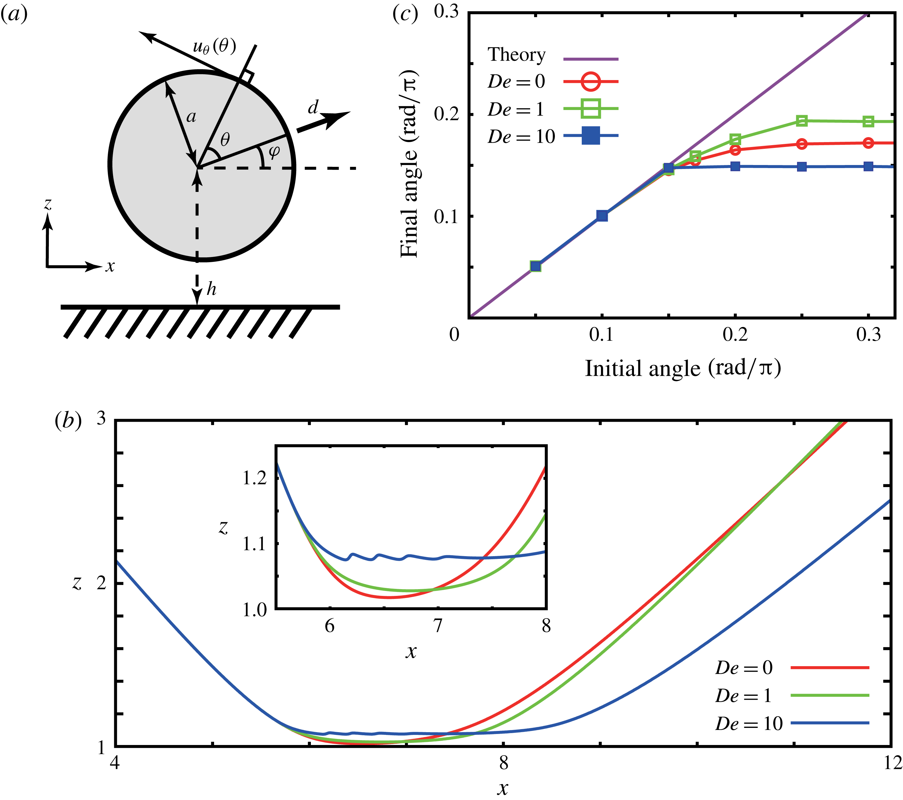
The first example swimmer is a spherical squirmer, which is driven via a tangential surface velocity profile on its surface. In particular, we consider a sphere of radius
 $a$
with its centre a height
 $h$
above an infinite plane wall at
 $z=0$
, and introduce a swimmer orientation vector
 $\boldsymbol{d}$
within the
 $xz$
plane, making an angle
 $\unicode[STIX]{x1D711}$
with the plane wall; see figure 2. The surface velocity profile is given by
 $$\begin{eqnarray}u_{\unicode[STIX]{x1D703}}(\unicode[STIX]{x1D703})=V\sin \unicode[STIX]{x1D703},\end{eqnarray}$$
where the angle
 $\unicode[STIX]{x1D703}$
is measured from the orientation vector
 $\boldsymbol{d}$
, as also depicted in figure 2. This swimmer is also known as a neutral squirmer (Ishikawa, Simmons & Pedley Reference Ishikawa, Simmons and Pedley2006), and is repelled by the wall in the absence of wall interactions (Ishimoto & Gaffney Reference Ishimoto and Gaffney2013).
(a) A schematic of the spherical squirmer. (b) Example swimmer trajectories near a wall with an enlarged view shown in the inset. (c) Relation of the initial and final scattering angles for wall scattering, including Newtonian theoretical predictions for shallow scattering.

The sphere radius and the surface velocity are non-dimensionalised to a unit radius and a non-dimensional velocity
 $V=3/2$
. Owing to this scaling, the non-dimensional swimming velocity in the absence of a wall becomes unity. The number of mesh elements on the swimmer surface is
 $N=2048$
, and the meshes are iteratively generated by the BEMLIB library accompanying Pozrikidis (Reference Pozrikidis2002). The discretisation for each time step is given by
 $\unicode[STIX]{x0394}t=1/400$
, and the constants of the wall interactions are set as
 $(g\unicode[STIX]{x1D707}/T,d/a)=(400,1/50)$
. The large scale of the interaction strength entails the repulsive force is very large once the swimmer is in the vicinity of the wall, while the small interaction length scale entails that the swimmer has to be very close to the wall to experience the repulsive force.
We performed numerical computations, changing the initial angle of attack and the Deborah number, which is the non-dimensional relaxation time, given by
 $De=\unicode[STIX]{x1D706}/T$
, where
 $T=3a/2V$
is the characteristic time scale of this system. In figure 2(b), the computed trajectories of the squirmer are plotted for an initial angle of attack
 $\unicode[STIX]{x1D711}_{init}=0.2\unicode[STIX]{x03C0}$
with the Deborah numbers
 $De\in \{0,1,10\}$
. It is found that the viscoelasticity weakly increases the surface repulsion and weakly influences the scattering angle and the duration that the swimmer remains near the wall. In particular, on varying the initial angles of attack for these swimmers, the relation between the initial and final scattering angles
 $(\unicode[STIX]{x1D711}_{init},\unicode[STIX]{x1D711}_{fin})$
is plotted in figure 2(c). In these simulations, the swimmer is initially located at
 $(x,z)=(0,5)$
and the final angles are obtained from the trajectory only once the simulation times reaches
 $50T$
, so that the swimmer is in the very far field of the wall. In the plots of figure 2(c), for the cases with shallow initial angles, the swimmer does not approach the area with wall interactions, and thus the scattering angles are well explained by the far-field point singularity theory,
 $$\begin{eqnarray}\unicode[STIX]{x1D711}_{fin}=\sqrt{\unicode[STIX]{x1D711}_{init}^{2}+1/64},\end{eqnarray}$$
provided by Spagnolie & Lauga (Reference Spagnolie and Lauga2012). Nonetheless, as the initial angle steepens, the final angles deviate from the shallow-angle theoretical prediction and vary non-monotonically with the Deborah number.
4.4 Bacterial swimmer
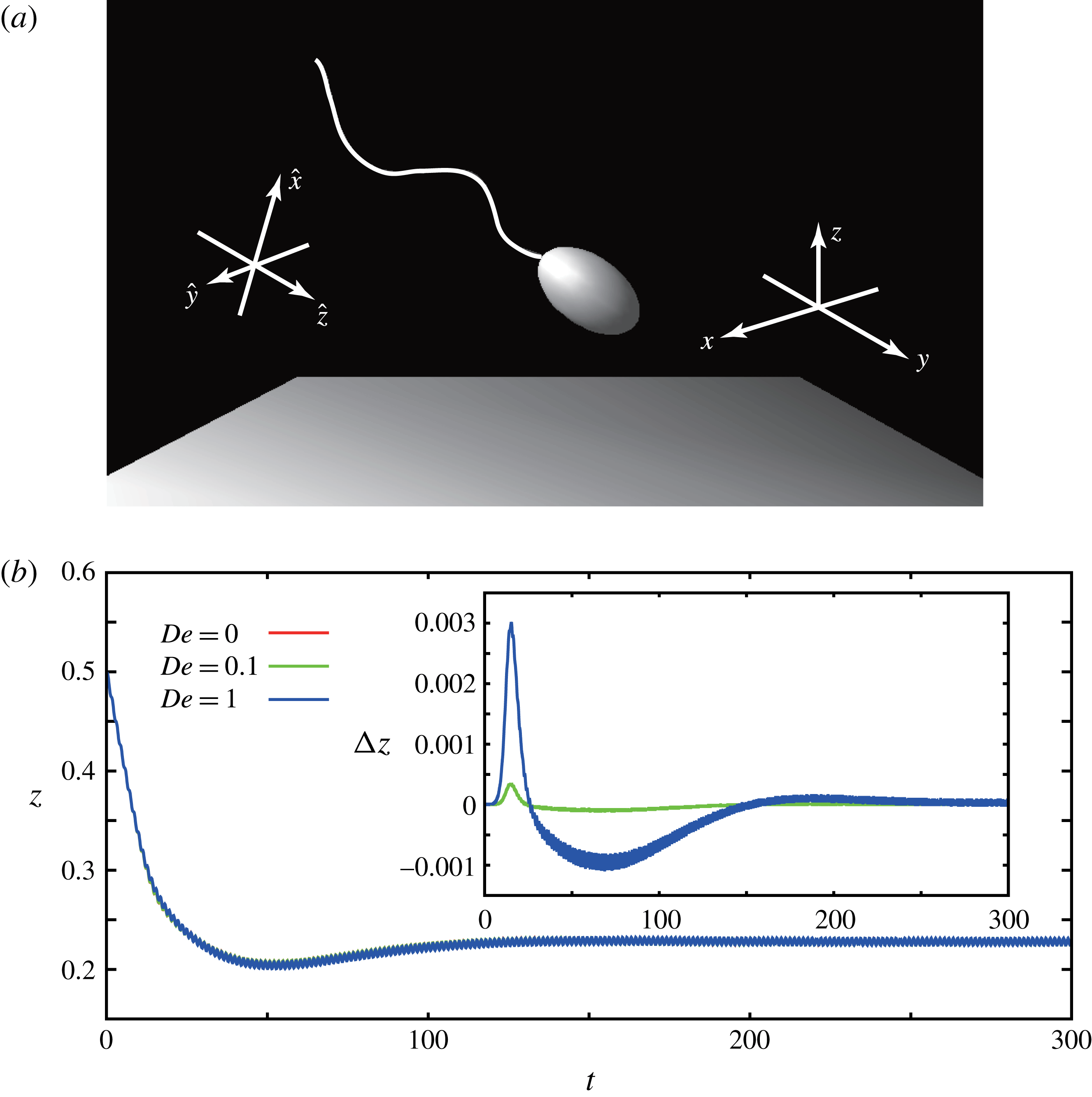
(a) A schematic of the monotrichous bacterial swimmer with its flagellum, together with the axes of the inertial and body-fixed reference frames and the underlying no-slip wall. (b) The time evolution of the separation distance from the proximal flagellum to the wall, with differences of
 $z$
from the
 $De=0$
case depicted for
 $De=0.1$
and
 $De=1$
in the inset.

The second example is a monotrichous bacterial swimmer, which is known to accumulate near a no-slip wall (Berke et al. Reference Berke, Turner, Berg and Lauga2008) and numerical simulations have shown that hydrodynamic interactions are sufficient to explain even the subtle aspects of this accumulation behaviour (Giacché, Ishikawa & Yamaguchi Reference Giacché, Ishikawa and Yamaguchi2010; Goto, Nakai & Aoki Reference Goto, Nakai and Aoki2010; Shum, Gaffney & Smith Reference Shum, Gaffney and Smith2010). Hence this example examines the extent to which viscoelastic effects may alter stable swimming near a surface, as opposed to the scattering of the previous example.
The virtual bacterium consists of a spheroidal cell body, whose polar radius and equatorial radius are, respectively,
 $a_{1}$
and
 $a_{2}$
, together with a single cylindrical flagellum of length
 $L$
and radius
 $r$
(figure 3
a). Following Shum et al. (Reference Shum, Gaffney and Smith2010), the flagellum waveform is taken to be a helical wave, and the centreline of the flagellum is given in terms of the body-fixed coordinates
 $(\hat{x}(\hat{z},t),{\hat{y}}(\hat{z},t),\hat{z})$
by
 $$\begin{eqnarray}\displaystyle & \displaystyle \hat{x}=A(1-\text{e}^{-k_{E}^{2}\hat{z}^{2}})\cos (k\hat{z}+\unicode[STIX]{x1D714}t), & \displaystyle\end{eqnarray}$$
 $$\begin{eqnarray}\displaystyle & \displaystyle {\hat{y}}=A(1-\text{e}^{-k_{E}^{2}\hat{z}^{2}})\sin (k\hat{z}+\unicode[STIX]{x1D714}t), & \displaystyle\end{eqnarray}$$
where
 $A$
is the amplitude of the helix,
 $k$
is the wavenumber and
 $\unicode[STIX]{x1D714}=2\unicode[STIX]{x03C0}/T$
is the angular velocity in terms of the time period
 $T$
. The parameter
 $k_{E}$
governs the scale of the initial increase in the flagellar envelope as the flagellum leaves its junction with the cell body at
 $\hat{\boldsymbol{x}}=\mathbf{0}$
. The functions (4.7) and (4.8) are defined for
 $\hat{z}\in [\hat{z}_{end},0]$
, where the coordinate of the flagellar distal end
 $\hat{z}_{end}<0$
is given by
 $$\begin{eqnarray}L=\int _{\hat{z}_{end}}^{0}\sqrt{1+\left(\frac{\text{d}\hat{x}}{\text{d}\hat{z}}\right)^{2}+\left(\frac{\text{d}{\hat{y}}}{\text{d}\hat{z}}\right)^{2}}\,\text{d}\hat{z}.\end{eqnarray}$$
In the simulation, the parameters of the model bacterium are those of optimal power efficiency, as obtained by Shum et al. (Reference Shum, Gaffney and Smith2010) and given by
 $a_{1}/L=0.154$
,
 $a_{2}/L=0.0922$
,
 $k_{E}L=10.0$
,
 $A/L=0.079$
,
 $kL/2\unicode[STIX]{x03C0}=1.953$
and
 $r/L=0.003$
. The system is non-dimensionalised using the flagellum length for the length scale
 $L$
, the flagellum rotation period for the time scale
 $T$
and the medium viscosity for the force scale, such that the non-dimensional viscosity is unity. Note however that, for the virtual bacterial model discussed by Shum et al. (Reference Shum, Gaffney and Smith2010), the flagellum rotates with a constant applied torque at its proximal end. In this study, in contrast, the flagellum motion is fully prescribed in the body-fixed frame by the functions (4.7) and (4.8), and the bacterial motion is therefore subject to the same kinematical problem as the squirmer case.
The surface meshes are generated as in Shum et al. (Reference Shum, Gaffney and Smith2010), with the head mesh constructed in the same way as the squirmer, with a subsequent stretching to generate the ellipsoidal head shape. The flagellum is meshed as a hexagonal tube with hemispherical caps at the ends, noting a small cell–flagellum gap is introduced in practice to numerically accommodate the relative motion of these surfaces as in previous studies (Shum et al.
Reference Shum, Gaffney and Smith2010; Ishimoto & Gaffney Reference Ishimoto and Gaffney2014a
). The total number of mesh elements on the swimmer surface is set to
 $N=494$
, and the discretisation for each time step is given by
 $\unicode[STIX]{x0394}t=1/400$
. The constants of the wall interactions are once more set to
 $(g\unicode[STIX]{x1D707}/T,d/L)=(400,1/50)$
.
We conducted numerical simulations with different Deborah numbers
 $De=\unicode[STIX]{x1D706}/T\in \{0,0.1,1\}$
. Note that at high Deborah numbers the forces and torques acting on the flagellum can differ substantially relative to the Newtonian case, and therefore the flagellar motion may change even if the internal torque generation is invariant. In such a highly elastic medium, the prescribed motion is in fact likely to be altered. In contrast to the previous idealised example of a squirmer, which we assumed can always maintain the prescribed deformation even with large elastic forces, here we focus on moderate values of the Deborah number. In figure 3(b), the time evolution of the distance from the wall boundary and the flagellar proximal end is plotted, and the differences are relatively minor, as particularly emphasised by the inset. The swimmer is initially located so that the flagellar proximal end is at
 $\boldsymbol{x}=(0,0,0.5)$
and its initial angle of attack relative to the wall is
 $0.2\unicode[STIX]{x03C0}$
. After the swimmer reaches the region where the wall interaction is significant, the cell body rotates away from the surface and the cell subsequently relaxes to stable swimming adjacent to the wall.
4.5 Sperm-like swimmer
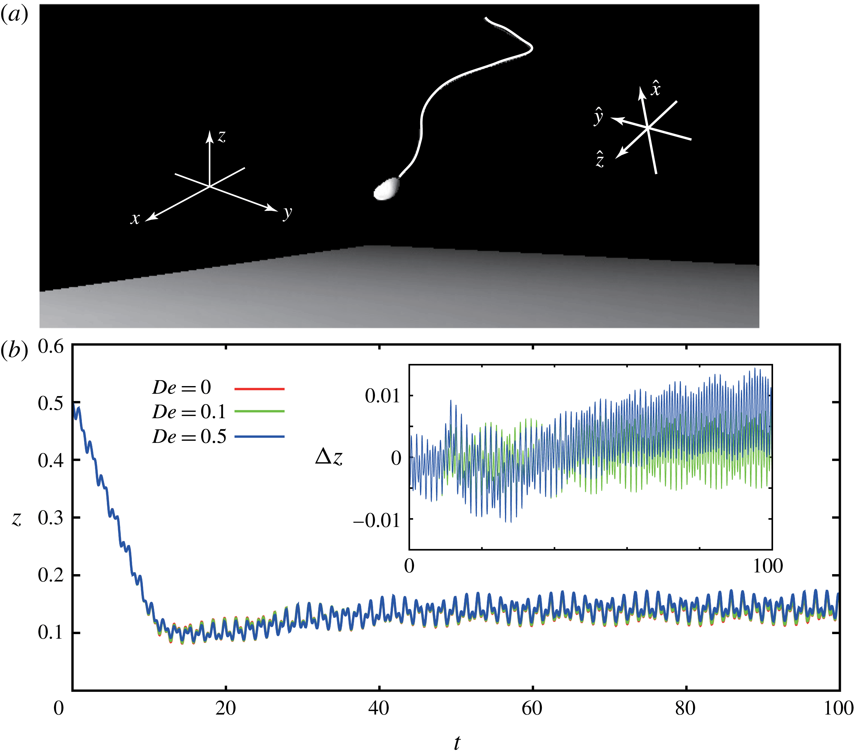
The third example swimmer is based on the morphology of a sperm, as illustrated in figure 4(a). Sperm in particular can be significantly affected by steric interactions when a sudden change in surface topography induces scattering (Kantsler et al. Reference Kantsler, Dunkel and Goldstein2013). In addition, it is theoretically predicted that steric interactions significantly influence the behaviour of a sperm cell near a boundary (Montenegro-Johnson, Gadelha & Smith Reference Montenegro-Johnson, Gadelha and Smith2015; Ishimoto & Gaffney Reference Ishimoto and Gaffney2015, Reference Ishimoto and Gaffney2016) where, in the latter citation, we examine the impact of viscoelasticity on beating cells adhered to a wall. Hence, here we consider how viscoelasticity impacts sperm swimming trajectories near a wall, which necessitates a viscoelastic boundary element method in the absence of the simplification associated with cell attachment.
(a) A schematic of the sperm-like swimmer with its flagellum above a no-slip plane boundary, together with body-fixed and inertial reference frame axes. (b) The time evolution of the separation distance of the cell body–flagellum junction from the wall, with differences of
 $z$
from the Newtonian case shown for
 $De=0.1$
and
 $De=0.5$
in the inset.

The virtual sperm-like swimmer has a flattened ellipsoidal head of human sperm and a cylindrical tail flagellum of length
 $L$
and radius
 $r$
. The head and tail morphologies are motivated by the human sperm geometrical model provided in Ishimoto & Gaffney (Reference Ishimoto and Gaffney2016), with a prescribed flagellar waveform that is an ellipsoidal helical wave (Smith et al.
Reference Smith, Gaffney, Blake and Kirkman-Brown2009a
), with an ellipsoidal cone envelope. The centreline of the flagellum is again defined as a function of
 $\hat{z}\in [\hat{z}_{end},0]$
, via
 $$\begin{eqnarray}\displaystyle & \hat{x}=\unicode[STIX]{x1D6FC}A|\hat{z}|\cos (k\hat{z}+\unicode[STIX]{x1D714}t), & \displaystyle\end{eqnarray}$$
 $$\begin{eqnarray}\displaystyle & {\hat{y}}=A|\hat{z}|\sin (k\hat{z}+\unicode[STIX]{x1D714}t), & \displaystyle\end{eqnarray}$$
where the parameter
 $\unicode[STIX]{x1D6FC}$
represents the major to minor aspect ratio of the elliptical cross-section through the enveloping cone of the flagellar beat, and
 $\hat{z}_{end}<0$
satisfies the fixed length constraint given by (4.9). The parameters used in the simulation are taken from Ishimoto & Gaffney (Reference Ishimoto and Gaffney2016), where morphological justification is provided; in particular we have
 $\unicode[STIX]{x1D6FC}=0.2$
,
 $A/L=0.2$
,
 $kL/2\unicode[STIX]{x03C0}=1.5$
and
 $r/L=0.0223$
. As with the bacterial swimmer, the system is non-dimensionalised using the flagellum length
 $L$
for the length scale, the beat period
 $T$
for the time scale and the medium viscosity for the force scale, such that the non-dimensional viscosity is unity.
The surface meshes are generated in a similar manner to the bacterial swimmer, details of which are provided in our previous studies (Ishimoto & Gaffney Reference Ishimoto and Gaffney2014a
, Reference Ishimoto and Gaffney2016). The total number of mesh elements on the swimmer surface is again
 $N=494$
, and the discretisation for each time step is given by
 $\unicode[STIX]{x0394}t=1/1600$
. The constants of the wall interactions are set to
 $(g\unicode[STIX]{x1D707}/T,d/L)=(400,1/50)$
while the swimmer is initially located so that the head–flagellum junction is at
 $\boldsymbol{x}=(0,0,0.5)$
and its angle of attack to the wall is
 $0.2\unicode[STIX]{x03C0}$
.
The results of similar numerical simulations with different Deborah numbers
 $De=\unicode[STIX]{x1D706}/T\in \{0,0.1,0.5\}$
are shown in figure 4(b) at integer times, or every beat cycle, with enlarged views inset. As with the bacterium, we do not consider large elasticity, because the prescribed waveform is unlikely to be conserved; instead, we consider moderate Deborah numbers once more. In figure 4(b), the time evolution of the distance between the wall and the head–flagellum junction is plotted, and the differences are relatively minor here too, as emphasised by the inset. Similarly to the bacterial case, the swimmer rotates on encountering the wall interactions, but the sperm head is slightly directed towards the wall. Furthermore, when the cell trajectory has asymptoted to boundary swimming, the conical envelope of the flagellum has rotated sufficiently downwards so as to induce intermittent wall interactions during the beat period. However, despite the fact that these interactions differ in the contribution to the momentum balances for the cell according to medium rheology, the actual trajectory of the sperm is not significantly altered on comparing swimming in a Newtonian fluid to that in a linear Maxwell fluid.
5 Magnetic swimmer
For a different application of the linear viscoelastic formulation, we consider a neutrally buoyant rigid helix with a permanent magnetisation, which can be induced to swim via an external magnetic field, as motivated by studies of externally guided helical microswimmers for many applications such as drug delivery (Qiu & Nelson Reference Qiu and Nelson2015).
5.1 Model
The magnetic swimmer is taken to be a rigid helix of length
 $L$
and radius
 $r$
, as considered in the section discussing the bacterial swimmer and depicted in figure 3. The centreline of the helix is given in terms of the body-fixed coordinates
 $(\hat{x}(\hat{z}),{\hat{y}}(\hat{z}))$
by
 $$\begin{eqnarray}\hat{x}=A\cos (k\hat{z})\quad \text{and}\quad {\hat{y}}=A\sin (k\hat{z}),\end{eqnarray}$$
where
 $A$
is the radius of the helix and
 $k$
is the wavenumber, with the latter giving the pitch of the helix. The
 $\hat{z}$
coordinate (
 $\hat{z}\in [\hat{z}_{end},0]$
) is related to the arclength via the fixed length constraint given by (4.9).
We assume the swimmer is a hard magnet with a fixed magnetisation
 $\boldsymbol{M}=M_{0}\hat{\boldsymbol{e}}_{x}$
along the body-fixed
 $\hat{x}$
axis. Therefore the helix experiences a force and torque in the presence of a magnetic flux density
 $\boldsymbol{B}$
given by (Qiu & Nelson Reference Qiu and Nelson2015)
 $$\begin{eqnarray}\displaystyle & \boldsymbol{F}_{ext}=C_{0}(\boldsymbol{M}\boldsymbol{\cdot }\unicode[STIX]{x1D735})\boldsymbol{B}, & \displaystyle\end{eqnarray}$$
 $$\begin{eqnarray}\displaystyle & \boldsymbol{T}_{ext}=C_{0}\boldsymbol{M}\times \boldsymbol{B}, & \displaystyle\end{eqnarray}$$
where
 $C_{0}$
is the constant magnetic volume of the object. We further assume the external magnetic flux density is that of a uniform rotating magnetic field given with respect to the inertial-frame basis via
 $$\begin{eqnarray}\boldsymbol{B}=B_{0}\left(\cos \left(\frac{2\unicode[STIX]{x03C0}t}{T}\right)\boldsymbol{e}_{x}+\sin \left(\frac{2\unicode[STIX]{x03C0}t}{T}\right)\boldsymbol{e}_{y}\right),\end{eqnarray}$$
where
 $B_{0}$
is constant and
 $T$
is the period of rotation. Note that such fields are commonly using to guide magnetic particles (Qiu & Nelson Reference Qiu and Nelson2015) and also that an inspection of (5.2) reveals that the magnetic force on the helix vanishes due to the spatial uniformity of the magnetic flux density.
5.2 Computational results
The effects of linear viscoelasticity can be treated by considering the torque balance equation. Similarly to the wall interaction case (4.4), we have
 $$\begin{eqnarray}\int _{S}\unicode[STIX]{x1D716}_{ipq}x_{p}f_{q}^{VE}+{\mathcal{L}}((T_{ext})_{i})=0,\end{eqnarray}$$
where we consider the linear Maxwell model,
 ${\mathcal{L}}=1+\unicode[STIX]{x1D706}\unicode[STIX]{x2202}/\unicode[STIX]{x2202}t$
, and the Deborah number is given by
 $De=\unicode[STIX]{x1D706}/T$
.
For the shape parameters, we set
 $A/L=0.05$
,
 $r/L=0.003$
and
 $kL/2\unicode[STIX]{x03C0}=10$
, which gives the pitch of the helix to be
 $0.2L$
. We proceed by non-dimensionalising the length, time and force scales such that in the non-dimensional model the swimmer length, time period and viscosity are given by
 $L=1$
,
 $T=1$
and
 $\unicode[STIX]{x1D707}=1$
, which results in a non-dimensionalised constant representing the strength of the magnetic torque, given by
 $F_{mag}=C_{0}M_{0}B_{0}(\unicode[STIX]{x1D707}L^{3}/T)$
. We also set the initial condition of the magnetic helix so that the body-fixed frame and the inertial reference frame coincide, and we denote the origin of the body-fixed frame relative to the inertial frame by
 $\boldsymbol{X}(t)$
. With these initial conditions, the swimmer experiences no torque at the initial time
 $t=0$
. The resulting boundary integral equations are analogous to those in figure 3 and are computed with
 $N=366$
mesh elements and the time discretisation
 $\unicode[STIX]{x0394}t/T=1/500$
.
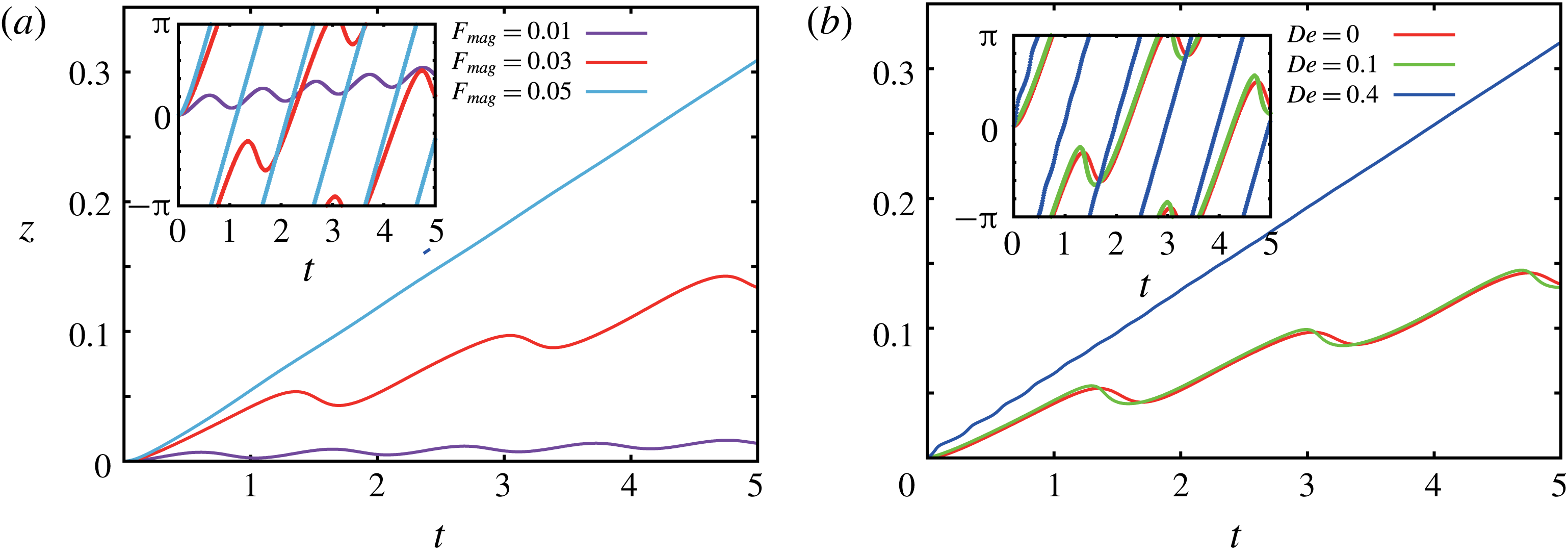
The dynamics of permanently magnetised swimmers. (a) The movement of the helical magnetic swimmer within a Newtonian fluid for a rotating magnetic flux density and varying non-dimensional magnetic torque,
 $F_{mag}$
. The inset indicates the time evolution of the orientation of the swimmer magnetisation vector, as measured by
 $\unicode[STIX]{x1D703}_{mag}$
, the angle between
 $\boldsymbol{e}_{x}$
and
 $\hat{\boldsymbol{e}}_{x}$
, measured from the
 $x$
axis. (b) Movement of the helical magnetic swimmer with a non-dimensional magnetic torque
 $F_{mag}=0.03$
in fluids with different Deborah numbers. The inset indicates the corresponding time evolution of the orientation of the magnetisation vector as in (a). The red curves in (a) and (b) are therefore the same.

We first consider the motion in a Newtonian fluid, and the time evolution of the helix is plotted in figure 5(a) with varying non-dimensional magnetic torque,
 $F_{mag}$
. The plots shows the
 $z$
component of the swimmer,
 $\boldsymbol{x}\boldsymbol{\cdot }\boldsymbol{e}_{z}$
, as a function of time, where
 $\boldsymbol{e}_{z}$
denotes the unit inertial-frame basis vector in the
 $z$
direction. In the inset, the orientation of the magnetisation vector is shown via a plot of
 $\unicode[STIX]{x1D703}_{mag}$
, the angle between
 $\boldsymbol{e}_{x}$
and
 $\hat{\boldsymbol{e}}_{x}$
, as measured from the
 $x$
axis. For a sufficiently strong magnetic torque, the helix rotation is slave to that of the external field (figure 5
a inset), and the helix moves along the
 $z$
axis at constant speed. However, for weaker magnetic torques, there is a phase difference between the magnetisation vector and the external magnetic flux density. Once this phase difference exceeds
 $\unicode[STIX]{x03C0}$
, the magnetisation vector then counter-rotates to relax to the external magnetic flux density. In turn, the helix also moves in the opposite direction, resulting in trajectories with oscillations (figure 5
a).
We then proceed to consider non-zero Deborah number, with the same initial conditions, and focus on swimming with
 $F_{mag}=0.03$
, which is insufficient to induce a rotation of the helix in a constant direction within a Newtonian fluid. Analogous plots of the position and the orientation of the magnetic swimmer are shown in figure 5(b) with increasing Deborah numbers. When
 $De=0.1$
, the phase difference between the magnetisation vector and the external magnetic vector is slightly suppressed, but nonetheless is still large enough to induce counter-rotation. Further increases of the Deborah number, however, amplify the effective torque that the swimmer experiences, and result in the magnetisation vector following the external magnetic field, and thus the swimmer rotates uniformly in time, with a dramatic increase in swimming propagation.
6 Conclusions
In this paper, we have considered the dynamics of a swimmer with arbitrary prescribed deformation in a negligible Reynolds-number, non-Newtonian linear Maxwell medium. Using the Stokeslet for this medium, and introducing a generalised reciprocal relation, we have derived the boundary integral equations for linear Maxwell flows, though other linear viscoelastic flows are readily considered, as detailed in appendix A. Under the assumptions of volume-conserving deformation, the single-layer boundary integral equations are also derived, together with the force and torque balance equations. In turn this provides, to our knowledge, a first formulation of the boundary element method for a swimmer in a linear Maxwell medium that only requires surface integration. One can immediately observe that this framework demonstrates that swimming dynamics in a linear Maxwell fluid is identical to that in Newtonian Stokes flow, if no net forces and torques are acting on the swimmer. This also provides a generalisation of Purcell’s scallop theorem (Purcell Reference Purcell1977) for Maxwell linear viscoelastic flows with arbitrary volume-conserving reciprocal motion; this result is also readily generalised to reciprocal, non-volume-conserving, deformations by including the double-layer formulation.
The exact agreement between predictions for flows and trajectories for swimmers in Newtonian media, on the one hand, and a linear Maxwell fluid, on the other, however, does break down when external forces are applied. Thus we investigated swimmer dynamics near a rigid wall, with a repulsive wall potential force acting on the swimmer, as motivated by the measurements of boundary–cell interactions by Klein et al. (Reference Klein, Clapp and Dickinson2003), novelly incorporating the impact of linear Maxwell viscoelasticity.
Using the boundary element method provided in this paper, we thus examined swimming trajectories within a linear Maxwell viscoelastic fluid for three example swimmers: a neutral spherical tangential squirmer, a virtual bacterium and a virtual sperm. For the spherical tangential squirmer, which is scattered by hydrodynamical wall interactions, the fluid viscoelasticity weakly enhances wall repulsion and affects the scattering angle. For the bacterium and sperm, which stably swim adjacent to the wall, viscoelasticity at moderate Deborah numbers does not significantly change the final stable swimming dynamics, even for the virtual sperm, which can continually experience wall interactions during a beat period while boundary swimming. Consequently we have an important null result that linear Maxwell viscoelasticity at moderate Deborah number does not alter flagellate–boundary dynamics given the waveform, even at surfaces with surface potentials. Hence our understanding of surface swimming that has been developed for Newtonian flows and standard waveforms observed from digital microscopy, as summarised in the introduction, immediately generalises. These results also support the ubiquitous simplification of using Newtonian simulation methods for sperm and bacterial motility in media well approximated by linear Maxwell viscoelasticity, such as the dilute methylcellulose solutions used as mucous analogues in sperm motility studies (Smith et al. Reference Smith, Gaffney, Gadêlha, Kapur and Kirkman-Brown2009b ).
As the second example case, we investigated motions of a magnetised helix under a rotating magnetic field, once more generalising to consider a linear Maxwell fluid, which demonstrated that the linear viscoelastic boundary element framework can also be applied to swimming via an external forcing as well as a prescribed shape deformation. In particular, we found that, with an intermediate strength of the magnetic induction, the model magnetic swimmer repeatedly rotates and counter-rotates within a Newtonian medium. However, in the presence of linear viscoelasticity, the swimmer is predicted to rotate at constant speed, following the external magnetic field, with a drastic increase in propagation, which illustrates that linear viscoelasticity can dramatically alter microswimmer dynamics. However, a systematic study, concerning the impact of the motion of the magnetic field, the shape of the swimmer, the details of the swimmer magnetisation and the influence of the external magnetic field, will be reported elsewhere.
Despite this example, the present framework cannot readily deal with coupled fluid–active structure problems for viscoelastic flow where the interface shape is an emergent property, since the generalisation of surface traction with viscoelasticity, that is
 $\boldsymbol{f}^{VE}$
in (3.21) and (3.22), does not possess a straightforward physical interpretation. Hence boundary element methods for such fluid–active structure problems in the context of linear viscoelastic fluids should be considered as a future study.
Nonetheless, the numerical techniques presented here allow one to model swimmer and particle trajectories with prescribed kinematics or external forces and torques. The framework can also readily accommodate the dynamics of small numbers of particles and swimmers via (4.3) and (4.4) for a range of linear viscoelastic constitutive laws, such as
 $$\begin{eqnarray}\unicode[STIX]{x1D706}\frac{\unicode[STIX]{x2202}\unicode[STIX]{x1D749}}{\unicode[STIX]{x2202}t}+\unicode[STIX]{x1D749}=2\unicode[STIX]{x1D707}\boldsymbol{D}+2\unicode[STIX]{x1D707}\unicode[STIX]{x1D6FE}\frac{\unicode[STIX]{x2202}\boldsymbol{D}}{\unicode[STIX]{x2202}t},\end{eqnarray}$$
where
 $\unicode[STIX]{x1D6FE}\geqslant 0$
is an additional viscoelastic response time, by noting the results in appendix A. Hence, in addition to allowing an analysis of the extent to which linear viscoelasticity impacts a diverse range of important microswimmers, as outlined here, the presented framework can be used to analyse particle–particle interactions (the underlying basis for understanding many-body effects) in active micrometre-scale linear viscoelastic rheology (Gomez-Solano & Bechinger Reference Gomez-Solano and Bechinger2015). Furthermore, any study using this linear viscoelasticity framework requires only a minimalistic generalisation of the classical boundary element method, a major advantage of the methodology.
Acknowledgements
K.I. is supported by JSPS-KAKENHI for Young Researchers (15H06314), Kyoto University for the Hakubi Project and Kyoto University Supporting Program for Interaction-based Initiative Team Studies (SPIRIS). K.I. acknowledges JSPS for a JSPS Overseas Research Fellowship. Elements of the simulations have been performed using the cluster computing system within the Research Institute for Mathematical Sciences (RIMS), and Institute for Information Management and Communication (IIMC), Kyoto University. The authors acknowledge anonymous referees for their comments that helped to improve the manuscript.
Appendix A. Boundary integral equations for a more general constitutive relation
Here, we derive the boundary element formulation for the more general constitutive relation,
 $$\begin{eqnarray}\unicode[STIX]{x1D706}\frac{\unicode[STIX]{x2202}\unicode[STIX]{x1D749}}{\unicode[STIX]{x2202}t}+\unicode[STIX]{x1D749}=:{\mathcal{L}}\unicode[STIX]{x1D749}=2\unicode[STIX]{x1D707}{\mathcal{M}}\boldsymbol{D}:=2\unicode[STIX]{x1D707}\boldsymbol{D}+2\unicode[STIX]{x1D707}\unicode[STIX]{x1D6FE}\frac{\unicode[STIX]{x2202}\boldsymbol{D}}{\unicode[STIX]{x2202}t},\end{eqnarray}$$
where
 $\unicode[STIX]{x1D706}$
and
 $\unicode[STIX]{x1D6FE}$
are viscoelastic response time scales. It is also straightforward to generalise the analysis presented here to multiple viscoelastic time scales, though we restrict ourselves to the above constitutive relation in the following.
First we require the reciprocal relation, whose derivation proceeds in the same way as in the main paper to reveal
 $$\begin{eqnarray}\frac{\unicode[STIX]{x2202}}{\unicode[STIX]{x2202}x_{j}}(({\mathcal{M}}u_{i}^{\prime }){\mathcal{L}}\unicode[STIX]{x1D70E}_{ij}-({\mathcal{M}}u_{i}){\mathcal{L}}\unicode[STIX]{x1D70E}_{ij}^{\prime })=0.\end{eqnarray}$$
We now use the viscoelastic Stokeslet satisfying
 ${\mathcal{M}}G_{ij}=G_{ij}^{S}$
. The resulting flow due to this singularity, located at the point
 $\boldsymbol{x}_{0}$
and of strength
 $\boldsymbol{q}$
, is governed by the relations
 $$\begin{eqnarray}{\mathcal{M}}G_{ij}=G_{ij}^{S}\quad \text{and}\quad {\mathcal{L}}P_{j}=P_{j}^{S},\end{eqnarray}$$
where the S superscript denotes the Stokes flow, Newtonian solution, with the velocity, pressure and stress fields given by
 $$\begin{eqnarray}u_{i}^{\prime }=\frac{1}{8\unicode[STIX]{x03C0}\unicode[STIX]{x1D707}}G_{ij}(\boldsymbol{x},\boldsymbol{x}_{0})q_{j},\quad p^{\prime }=\frac{1}{8\unicode[STIX]{x03C0}}P_{j}q_{j},\quad \unicode[STIX]{x1D70E}_{ij}^{\prime }=\frac{1}{8\unicode[STIX]{x03C0}}T_{ijk}q_{k}.\end{eqnarray}$$
The resulting momentum-balance equation is
 $$\begin{eqnarray}{\mathcal{L}}\unicode[STIX]{x1D70E}_{ij}^{\prime }=-\frac{1}{8\unicode[STIX]{x03C0}}{\mathcal{L}}P_{m}q_{m}+{\mathcal{M}}D_{ij}=-\frac{1}{8\unicode[STIX]{x03C0}}P_{m}^{S}q_{m}+\frac{1}{8\unicode[STIX]{x03C0}}\left(\frac{\unicode[STIX]{x2202}G_{ip}^{S}}{\unicode[STIX]{x2202}x_{j}}+\frac{\unicode[STIX]{x2202}G_{jp}^{S}}{\unicode[STIX]{x2202}x_{i}}\right)q_{p}=\unicode[STIX]{x1D70E}_{ij}^{\prime S},\end{eqnarray}$$
where the right-hand side is the stress tensor of a Stokes flow corresponding to a point force of strength
 $\boldsymbol{q}$
at the point
 $\boldsymbol{x}_{0}$
. Following the derivation of the boundary integral equation in the main text, but now with the constitutive relation
 ${\mathcal{L}}\unicode[STIX]{x1D749}=2\unicode[STIX]{x1D707}{\mathcal{M}}\boldsymbol{D}$
, one finds
 $$\begin{eqnarray}u_{p}^{VE}:={\mathcal{M}}u_{p}(\boldsymbol{x}_{0})=-\frac{1}{8\unicode[STIX]{x03C0}\unicode[STIX]{x1D707}}\int _{S}G_{ip}^{S}({\mathcal{L}}\unicode[STIX]{x1D70E}_{ij})\boldsymbol{n}_{j}\,\text{d}S+\frac{1}{8\unicode[STIX]{x03C0}}\int _{S}({\mathcal{M}}u_{i})T_{ipj}^{S}\boldsymbol{n}_{j}\,\text{d}S.\end{eqnarray}$$
Similarly, the single-layer boundary integral equation for a volume-preserving swimmer becomes
 $$\begin{eqnarray}u_{p}^{VE}(\boldsymbol{x}_{0})=-\frac{1}{8\unicode[STIX]{x03C0}\unicode[STIX]{x1D707}}\int _{S}G_{ip}^{S}(\boldsymbol{x},\boldsymbol{x}_{0})f_{i}^{VE}(\boldsymbol{x})\,\text{d}S_{\boldsymbol{ x}}.\end{eqnarray}$$
The force and torque balances remain unchanged. For instance, for the single-layer formalism, in the presence of an external wall interaction given by
 $\boldsymbol{f}_{wall}$
, one has
 $$\begin{eqnarray}\int _{S}f_{i}^{VE}\,\text{d}S_{\boldsymbol{ x}}+{\mathcal{L}}\int _{S}(f_{wall})_{i}\,\text{d}S=0,\quad \int _{S}\unicode[STIX]{x1D716}_{ipq}x_{p}f_{q}^{VE}\,\text{d}S_{\boldsymbol{ x}}+{\mathcal{L}}\int _{S}\unicode[STIX]{x1D716}_{ipq}x_{p}(f_{wall})_{q}\,\text{d}S=0,\end{eqnarray}$$
where
 $f_{i}^{VE}={\mathcal{L}}(\unicode[STIX]{x1D70E}_{ij}-\unicode[STIX]{x1D70E}_{ij}^{\ast })\boldsymbol{n}_{j}$
, with
 $\unicode[STIX]{x1D70E}_{ij}^{\ast }$
the stress tensor of a fictitious flow in the cell interior.
Hence to find trajectories for deformation swimming, or more generally the movement of a particle under an external force, in a linear viscoelastic fluid with the constitutive relation
 ${\mathcal{L}}\unicode[STIX]{x1D749}=2\unicode[STIX]{x1D707}{\mathcal{M}}\boldsymbol{D}$
, one proceeds as in the main text, except that, at each iteration, one must also use information from the previous time point (or initial conditions at the first time step) to determine
 ${\mathcal{M}}\boldsymbol{u}(\boldsymbol{x}_{0})$
in terms of the unknowns,
 $\boldsymbol{U}$
and
 $\unicode[STIX]{x1D734}$
. The former is the velocity of a point in the body-fixed frame (the head–tail junction for simulations with bacteria and sperm is often used, for instance) and the latter is the angular velocity of the body-fixed frame relative to the inertial fixed frame around this point.