1 Introduction
An immiscible dispersion of liquid drops in another liquid medium is ubiquitous in a wide variety of applications, ranging from food and material processing to pharmaceutical industries and petroleum refineries (Barnes Reference Barnes1994; Eow & Ghadiri Reference Eow and Ghadiri2002). These dispersions, commonly known as emulsions, can also be alternatively generated in controlled laboratory environments, following state-of-the art microfluidic techniques (Anna, Bontoux & Stone Reference Anna, Bontoux and Stone2003; Haliburton et al. Reference Haliburton, Kim, Clark, Sperling, Weitz and Abate2017). Irrespective of the specific applications and the pertinent physical scales based on the same, variations in the microstructures and morphologies of the individual drops in the dispersed phase may lead to drastic alterations in the bulk physicochemical properties of the emulsion (Puyvelde, Velankar & Moldenaers Reference Puyvelde, Velankar and Moldenaers2001; Tucker & Moldenaers Reference Tucker and Moldenaers2002). In addition, the application of external stresses has proved to be immensely useful in modifying the distribution, deformation and motion of the individual constituents of an emulsion.
In suspension mechanics, the bulk-scale description of a dispersion is often provided by considering an effective continuous medium. Physically, the perturbation in flow, due to the stresses exerted on the drops, affects the dissipation of energy by the continuous fluid. Consequently, the stress response of the bulk mixture deviates from that of a Newtonian fluid (Guazzelli & Morris Reference Guazzelli and Morris2011). Taylor (Reference Taylor1932) was the first to theoretically predict the contribution of the drop phase in increasing the effective viscosity of a dilute emulsion under an imposed linear flow. Later, it was found that the deformable nature of the suspended drops can not only impart an elastic nature to the emulsion rheology (Schowalter, Chaffey & Brenner Reference Schowalter, Chaffey and Brenner1968), but also may render a shear-thinning property (Barthès-Biesel & Acrivos Reference Barthès-Biesel and Acrivos1973) to the same.
One of the most promising techniques for manipulation of rheological properties of an emulsion is the use of an electric field (Pan & McKinley Reference Pan and McKinley1997; Ha & Yang Reference Ha and Yang2000; Na et al. Reference Na, Aida, Sakai, Kakuchi and Orihara2009). Electrohydrodynamic effects can deform a drop in an oblate or prolate spheroidal shape, depending on a combination of the electrical properties of the dispersed and continuous phases (Taylor Reference Taylor1966; Xu et al. Reference Xu, Li, Lowengrub and Zhao2006; Esmaeeli & Sharifi Reference Esmaeeli and Sharifi2011; Thaokar Reference Thaokar2012; Lanauze, Walker & Khair Reference Lanauze, Walker and Khair2015). In the case of leaky dielectric fluids, an electric field also induces a tangential flow around the drop (Saville Reference Saville1997). The electrohydrodynamic flow and drop deformation may get further affected by the presence of finite charge convection at the interface (Feng Reference Feng1999; Xu & Homsy Reference Xu and Homsy2006; Das & Saintillan Reference Das and Saintillan2016; Yariv & Almog Reference Yariv and Almog2016), with a possible consequence of breaking the fore–aft symmetry of a sedimenting drop (Bandopadhyay et al. Reference Bandopadhyay, Mandal, Kishore and Chakraborty2016). These findings have been extended to address droplet electrohydrodynamics in Poiseuille flow (Mandal, Bandopadhyay & Chakraborty Reference Mandal, Bandopadhyay and Chakraborty2016b ). The net effect of alteration of the flow physics in and around an individual drop (Allan & Mason Reference Allan and Mason1962; Maehlmann & Papageorgiou Reference Maehlmann and Papageorgiou2009) may culminate in the form of an altered rheology of the emulsion (Ha & Yang Reference Ha and Yang2000; Fernàndez Reference Fernàndez2008), in a rather non-intuitive manner.
Vlahovska (Reference Vlahovska2011) established a theoretical model depicting the influence of drop-level flow dynamics and deformation on the electrorheology of a dilute emulsion. That study considered a uniform electric field in the direction of the velocity gradient and analysed the combined interplay among the flow and electric field in the limits of weak flow and highly viscous drops. Charge convection was neglected in the weak flow limit. The orientation of the deformed drop along the flow direction was found responsible for the shear-thinning effect due to reduction in the flow resistance. Similarly an emulsion is likely to exhibit a shear-thickening property when a drop elongates orthogonally to the flow direction. Apart from the shear-rate-dependent rheology, the electric-field-induced compression or elongation of drops results in an additional tension along the streamlines. As a consequence, normal stress differentials are created, similar to polymeric liquids (Bird, Armstrong & Hassager Reference Bird, Armstrong and Hassager1987). Later Mandal & Chakraborty (Reference Mandal and Chakraborty2017a ) and Mandal et al. (Reference Mandal, Sinha, Bandopadhyay and Chakraborty2018) revealed the role of charge convection in modifying the bulk rheology, using an asymptotic analysis. Subsequently, they showed (Mandal & Chakraborty Reference Mandal and Chakraborty2017b ) that application of an electric field in the shearing plane and along a direction tilted to that of the flow can give rise to many non-intuitive bulk rheological properties of an emulsion, especially the existence of an electrical component of the effective shear viscosity in the absence of drop deformation, which makes it deviate significantly from the classical findings of Taylor (Reference Taylor1932).
In many industrial applications, emulsion stabilizers act as surface-active agents and reduce the interfacial tension after being adsorbed at the interface (Fischer & Erni Reference Fischer and Erni2007). Under dynamic conditions, the presence of these surface-active agents or surfactants results in Marangoni stresses, altering the state of interfacial force balance. Reported experiments have revealed the significant role of surfactants in the deformation of drops and the bulk rheology of an emulsion (Velankar et al. Reference Velankar, Van Pyuvede, Mewis and Moldenaers2001; Hu & Lips Reference Hu and Lips2003; Jeon & Macosko Reference Jeon and Macosko2003; Velankar et al. Reference Velankar, Van Puyvelde, Mewis and Moldenaers2004). To analyse the specific physical phenomena responsible for such behaviour, both analytical and numerical investigations have been conducted (Stone & Leal Reference Stone and Leal1990; Milliken, Stone & Leal Reference Milliken, Stone and Leal1993; Li & Pozrikidis Reference Li and Pozrikidis1997; Vlahovska, Loewenberg & Blawzdziewicz Reference Vlahovska, Loewenberg and Blawzdziewicz2005; Vlahovska, Bławzdziewicz & Loewenberg Reference Vlahovska, Bławzdziewicz and Loewenberg2009). These analyses show that the surfactant effects are mostly governed by the competing processes of surface convection, dilution and tip streaming. Several factors, such as the viscosity contrast of the drop–matrix fluid pair, local gradient in surface tension, initial surface tension and the flow strength, control the relative importance of the influencing mechanisms.
The effect of surfactants on electrically modulated drops has not been extensively studied (Ha & Yang Reference Ha and Yang1995; Teigen & Munkejord Reference Teigen and Munkejord2010; Nganguia et al. Reference Nganguia, Young, Vlahovska, Bławzdziewcz, Zhang and Lin2013; Ervik et al. Reference Ervik, Penne, Hellesø, Munkejord and Müller2018; Poddar et al. Reference Poddar, Mandal, Bandopadhyay and Chakraborty2018, Reference Poddar, Mandal, Bandopadhyay and Chakraborty2019). The electrorheology of concentrated emulsions in the presence of non-ionic surfactants has only been experimentally investigated by Ha, Moon & Yang (Reference Ha, Moon and Yang1999). However, a theoretical understanding of the physical processes associated with drop-scale flow physics and its connection to the bulk rheology of the effective fluid mixture remains elusive. Thus, in the present work, we attempt to unveil the complicated interconnection between the surfactant covering a drop surface, the electric field and the imposed linear shear flow, towards influencing the effective rheology. Considering a non-ionic, bulk insoluble surfactant coating the surface of a deformable viscous drop, dispersed in an electrically actuated emulsion, we adopt a comprehensive three-dimensional framework and analyse the problem through an asymptotic approach, in order to bring out the new physics of a complex non-trivial interplay of surfactant-induced transport and electromechanics over interfacial scales, as elucidated subsequently.
By accounting for the interfacial tension gradients due to the surfactants in a generic theoretical formalism, the present study stands apart from the reported literature on electrohydrodynamics of droplets. This may be attributed to a non-trivial interplay with the hydrodynamic and the Maxwell stresses that are implicitly connected with the surfactant dynamics, as mediated by the incipient flow field. This coupled interplay gets aptly manifested in the bulk rheological parameters, such as the effective viscosity and normal stress differences, in the various asymptotic orders of the analysis, which has not yet been unraveled in the literature. Our results further indicate that under the combined action of a tilted electric field and linear shear, the surfactant-induced Marangoni stresses modify the flow field around the drop in a diverse fashion, which cannot be predicted by a simple linear superposition of the individual governing processes, because of their implicit coupling. These alterations in the flow field, due to the interplay of competing physical mechanisms, lead to a non-intuitive shift of the peak surfactant accumulation from the plane of shear to a plane orthogonal to it. We portray such interconnected physical phenomena through a unique phase diagram. This phase map displays different critical tilt angle of the electric field and its dependence on the Mason number, the latter denoting the strength of the electrical stress relative to the hydrodynamic stress. For similar reasons, there exist unique critical shear rates relative to the electrical stresses
 $(\bar{G}_{cr})$
, for which the Marangoni effects surprisingly vanish, despite the existence of surfactant gradients. Such occurrence of a critical state is phenomenologically distinct from the critical shear rates obtained previously by Mandal & Chakraborty (Reference Mandal and Chakraborty2017b
), in the context of a surfactant-free drop. We also obtain new discriminating factors, involving the relevant electrical property ratios and the electric field configuration, which govern the critical shear rates
 $(\bar{G}_{cr})$
. Consequently, the bulk emulsion viscosity can either increase or decrease, depending on the electrical conductivity and permittivity ratios of the droplet and carrier phases. Finally, we show that depending on the tilt angle of the applied electric field, the elastic behaviour of the emulsion, interpreted through normal stress differences, gets significantly altered due to the presence of interfacial tension gradients brought about by the surfactant distribution.
2 Physical description
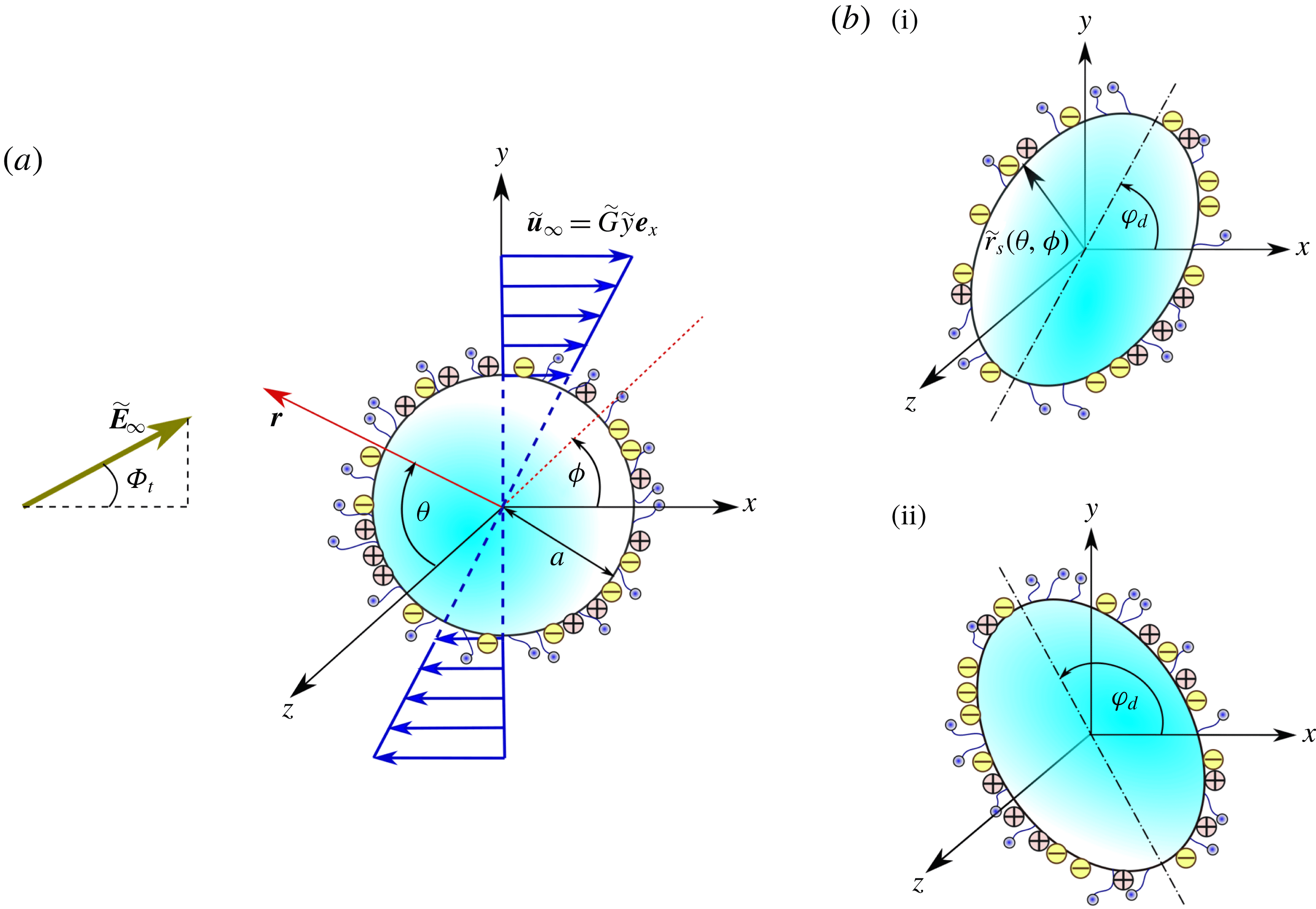
We consider a model emulsion where a drop of radius
 $a$
is dispersed in a background linear shear flow of the continuous phase along the
 $x$
direction given by
 $\widetilde{u}_{\infty }=\widetilde{G}\,\widetilde{y}$
. Here
 $\widetilde{G}$
is the uniform shear rate on the external fluid flow in the far stream. The drop is acted upon by a uniform-magnitude direct current electric field
 $\widetilde{\boldsymbol{E}}_{\infty }$
with a tilt angle
 $\unicode[STIX]{x1D6F7}_{t}$
in the plane of shear. In addition, the drop surface is covered with non-ionic surfactant molecules. The scenario is shown schematically in figure 1(a). When the drop surface is uncontaminated, the drop–matrix interface has a uniform surface tension
 $\widetilde{\unicode[STIX]{x1D6FE}}_{cl}$
. The presence of surface-active agents at this interface lowers this surface tension. In the quiescent condition, the surfactants have a uniform surface concentration of
 $\widetilde{\unicode[STIX]{x1D6E4}}_{eq}$
. Under the simultaneous action of the background flow and the electric field, the equilibrium distribution of the surfactants gets disrupted and the concentration distribution in the dynamic condition is given as
 $\widetilde{\unicode[STIX]{x1D6E4}}(\unicode[STIX]{x1D703},\unicode[STIX]{x1D719})$
. Depending on the flow behaviour and surface properties, the drop surface may deform to an ellipsoidal shape with its major axis being aligned with the
 $x$
direction at an angle
 $\unicode[STIX]{x1D711}_{d}$
. Two of the many possible configurations of the deformed drop in the
 $x{-}y$
plane are shown in figure 1(b). A body-fitted coordinate system fixed at the drop centroid is also shown in the figure. The drop-phase physical properties are denoted as viscosity (
 $\unicode[STIX]{x1D707}_{d}$
), electrical conductivity (
 $\unicode[STIX]{x1D70E}_{d}$
) and dielectric permittivity (
 $\unicode[STIX]{x1D716}_{d}$
), while the corresponding quantities for the outer continuous phase are denoted with the subscript ‘
 $d$
’ replaced with ‘
 $c$
’. We assume that the drop is neutrally buoyant in the continuous fluid, i.e. the densities of the two media are nearly equal (
 $\unicode[STIX]{x1D70C}_{d}\approx \unicode[STIX]{x1D70C}_{c}$
).
Schematic description of a deformable viscous drop being acted upon by a tilted electric field and background linear shear flow. The drop is covered with non-ionic surfactant molecules and interfacial charges accumulate on its surface. (a) The initial undeformed condition of the drop. Under the action of the external fields the drop may deform with an inclination angle
 $\unicode[STIX]{x1D711}_{d}$
as shown in (b). Two of the many possible configurations with
 $\unicode[STIX]{x1D711}_{d}<\unicode[STIX]{x03C0}/2$
and
 $\unicode[STIX]{x1D711}_{d}>\unicode[STIX]{x03C0}/2$
are shown as configurations (i) and (ii), respectively.

As a first step towards understanding the drop-scale flow dynamics, we neglect the interaction between the drops and assume that the drop-phase volume fraction
 $\unicode[STIX]{x1D708}$
to be in the dilute limit (
 $\unicode[STIX]{x1D708}\ll 1$
, where
 $\unicode[STIX]{x1D708}$
is the drop-phase concentration in the emulsion). It is important to note that the reported literature from the rheology community has primarily focused on the linear viscoelastic response of these emulsions when subjected to an oscillatory linear shear (e.g. Palierne Reference Palierne1990; Bousmina Reference Bousmina1999). These analyses are based on the consideration that the flow is time-dependent from an Eulerian perspective. In stark contrast, the present work is based on the assumption that the flow is steady from an Eulerian reference frame, in line with the works of Taylor (Reference Taylor1932) and Schowalter et al. (Reference Schowalter, Chaffey and Brenner1968). Thus the present study remains applicable to the steady shear conditions typically found in many experimental studies (Bentley & Leal Reference Bentley and Leal1986; Velankar et al.
Reference Velankar, Van Puyvelde, Mewis and Moldenaers2004).
3 Mathematical description
In order to derive the dimensionless governing differential equations depicting the above physical problem we adopt the following characteristic values as reference scales for the different variables: (i) length
 ${\sim}a$
, (ii) velocity
 ${\sim}\widetilde{G}a$
, (iii) electric field
 ${\sim}\widetilde{E}_{\infty }$
and (iv) surfactant concentration
 ${\sim}\widetilde{\unicode[STIX]{x1D6E4}}_{eq}$
. The relative importance of the characteristic electric stress
 $({\sim}\unicode[STIX]{x1D716}_{c}\widetilde{E}_{\infty }^{2})$
and hydrodynamic stress
 $({\sim}\unicode[STIX]{x1D707}_{c}\widetilde{G})$
is embodied in the dimensionless quantity defined as the Mason number,
 $M=\unicode[STIX]{x1D716}_{c}\widetilde{E}_{\infty }^{2}/\unicode[STIX]{x1D707}_{c}\widetilde{G}$
. From this non-dimensionlization scheme we obtain the following important property ratios appearing in the problem formulation: electrical conductivity ratio,
 $R=\unicode[STIX]{x1D70E}_{d}/\unicode[STIX]{x1D70E}_{c}$
; dielectric permittivity ratio,
 $S=\unicode[STIX]{x1D716}_{d}/\unicode[STIX]{x1D716}_{c}$
; and viscosity ratio,
 $\unicode[STIX]{x1D706}=\unicode[STIX]{x1D707}_{d}/\unicode[STIX]{x1D707}_{c}$
.
3.1 Governing equations and boundary conditions
We assume that the concentration of the surfactants adsorbed on the drop interface is small so that it does not deviate significantly from the equilibrium concentration. Thus the surface tension
 $(\widetilde{\unicode[STIX]{x1D6FE}})$
can be related to the local surfactant concentration by the relation (Stone Reference Stone1990; Leal Reference Leal2007)
 $$\begin{eqnarray}\widetilde{\unicode[STIX]{x1D6FE}}(\widetilde{\unicode[STIX]{x1D6E4}})=\widetilde{\unicode[STIX]{x1D6FE}}_{cl}-R_{g}T\,\widetilde{\unicode[STIX]{x1D6E4}},\end{eqnarray}$$
where
 $\widetilde{\unicode[STIX]{x1D6FE}}_{cl}$
is the surface tension of a clean (surfactant-free) drop,
 $T$
stands for the absolute temperature and
 $R_{g}$
denotes the ideal gas constant. Here onwards we denote the variables in their dimensionless forms and drop the tilde symbol from the notations. Based on the present considerations of a steady-state process and bulk insoluble surfactant molecules, the surfactant transport is governed by the following convection–diffusion equation (Leal Reference Leal2007):
 $$\begin{eqnarray}Pe_{S}\unicode[STIX]{x1D735}_{S}\boldsymbol{\cdot }(\boldsymbol{u}_{S}\unicode[STIX]{x1D6E4})=\unicode[STIX]{x1D6FB}_{S}^{2}\unicode[STIX]{x1D6E4},\end{eqnarray}$$
where
 $Pe_{S}=a^{2}\,\widetilde{G}/D_{S}$
is the surface Péclet number which represents the relative importance of convection and diffusion at the drop interface. It is to be noted that although the above surfactant transport equation has the same mathematical form as the one reported previously in the absence of electrical effects (Das, Mandal & Chakraborty Reference Das, Mandal and Chakraborty2017a
; Das et al.
Reference Das, Mandal, Som and Chakraborty2017b
), the electrical effects implicitly affect the surface transport through the surface velocity
 $(\boldsymbol{u}_{S})$
, and thus the surfactant distribution is expected to become altered due to the electrical effects.
In order to model the electrical effects, we consider the situation when both the drop and continuous phases are of a leaky dielectric nature and adopt the Taylor–Melcher leaky dielectric model (Melcher & Taylor Reference Melcher and Taylor1969; Saville Reference Saville1997; Vlahovska Reference Vlahovska2019). According to this model, the electric potentials in the drop and continuous phase
 $(\unicode[STIX]{x1D713}_{d},\unicode[STIX]{x1D713}_{c})$
satisfy
 $$\begin{eqnarray}\unicode[STIX]{x1D6FB}^{2}\unicode[STIX]{x1D713}_{d,c}=0.\end{eqnarray}$$
Apart from the usual boundedness of potential in and around the drop, the matching condition at the drop interface and the condition of uniformly imposed electric field at the far stream (i.e.
 $r\rightarrow \infty$
,
 $\unicode[STIX]{x1D735}\unicode[STIX]{x1D713}_{c}=-\boldsymbol{E}_{\infty }$
), the interfacial charge balance turns out to be an important condition for the present problem. In the quasi-steady state this reads (Xu & Homsy Reference Xu and Homsy2006)
 $$\begin{eqnarray}\text{at}~r=r_{S}(\unicode[STIX]{x1D703},\unicode[STIX]{x1D719}),\quad \boldsymbol{n}\boldsymbol{\cdot }(R\unicode[STIX]{x1D735}\unicode[STIX]{x1D713}_{d}-\unicode[STIX]{x1D735}\unicode[STIX]{x1D713}_{c})=-Re_{E}\unicode[STIX]{x1D735}_{S}\boldsymbol{\cdot }(q_{S}\boldsymbol{u}_{S}),\end{eqnarray}$$
where
 $\boldsymbol{n}$
is the unit vector in the normal direction at the drop surface and
 $\unicode[STIX]{x1D735}_{S}$
is the surface gradient operator
 $(\unicode[STIX]{x1D735}_{S}=(\boldsymbol{I}-\boldsymbol{n}\boldsymbol{n})\boldsymbol{\cdot }\unicode[STIX]{x1D735})$
. Here
 $Re_{E}=\unicode[STIX]{x1D716}_{c}\widetilde{G}/\unicode[STIX]{x1D70E}_{c}$
is the electrical Reynolds number quantifying the relative importance of the charge relaxation time scale and charge convection time scale. Charge convection (3.4a,b
) implies that the charge distribution and in effect the electric potential are coupled with the velocity field. Since the velocity field is affected by the surfactant non-uniformity, the electrical potential is also influenced by the surfactants, following (3.4a,b
).
Neglecting the inertial effect in the creeping flow limit (where hydrodynamic Reynolds number
 $Re=\unicode[STIX]{x1D70C}_{c}\widetilde{G}a^{2}/\unicode[STIX]{x1D707}_{c}\ll 1$
), the hydrodynamics can be described by the following equations (Happel & Brenner Reference Happel and Brenner1981):
 $$\begin{eqnarray}-\unicode[STIX]{x1D735}p_{d}+\unicode[STIX]{x1D706}\unicode[STIX]{x1D6FB}^{2}\boldsymbol{u}_{d}=0,\quad \unicode[STIX]{x1D735}\boldsymbol{\cdot }\boldsymbol{u}_{d}=0\quad \text{and}\quad -\unicode[STIX]{x1D735}p_{c}+\unicode[STIX]{x1D6FB}^{2}\boldsymbol{u}_{c}=0,\quad \unicode[STIX]{x1D735}\boldsymbol{\cdot }\boldsymbol{u}_{c}=0.\end{eqnarray}$$
Similar to the electric potential, the pressure and velocity both in the drop as well as in the outer region must be bounded and they are continuous at the drop interface. Also the fluid velocity at the far stream matches with the applied background flow velocity, i.e.
 $r\rightarrow \infty ,\boldsymbol{u}_{c}=\boldsymbol{V}_{\infty }$
. Again in the quasi-steady state the normal velocity at the interface becomes zero, i.e. at
 $r=r_{S}(\unicode[STIX]{x1D703},\unicode[STIX]{x1D719})~\boldsymbol{u}_{d}\boldsymbol{\cdot }\boldsymbol{n}=\boldsymbol{u}_{c}\boldsymbol{\cdot }\boldsymbol{n}=0$
. Finally the interface stress balance can be expressed as
 $$\begin{eqnarray}\text{at}~r=r_{S}(\unicode[STIX]{x1D703},\unicode[STIX]{x1D719}),\quad \unicode[STIX]{x27E6}\boldsymbol{T}^{H}\unicode[STIX]{x27E7}+M\,\unicode[STIX]{x27E6}\boldsymbol{T}^{E}\unicode[STIX]{x27E7}=\frac{1}{Ca}(\unicode[STIX]{x1D735}\boldsymbol{\cdot }\boldsymbol{n})\boldsymbol{n}+\underbrace{Ma\,[(1-\unicode[STIX]{x1D6E4})(\unicode[STIX]{x1D735}\boldsymbol{\cdot }\boldsymbol{n})\boldsymbol{n}+\unicode[STIX]{x1D735}_{S}\unicode[STIX]{x1D6E4}]}_{Marangoni\,stress},\end{eqnarray}$$
where
 $\unicode[STIX]{x27E6}\unicode[STIX]{x1D74C}\unicode[STIX]{x27E7}$
denotes the jump of a variable
 $\unicode[STIX]{x1D74C}$
at the interface (e.g.
 $\unicode[STIX]{x27E6}\unicode[STIX]{x1D74C}\unicode[STIX]{x27E7}=\unicode[STIX]{x1D74C}_{c}-\unicode[STIX]{x1D74C}_{d}$
);
 $\boldsymbol{T}^{H,E}=\boldsymbol{n}\boldsymbol{\cdot }\unicode[STIX]{x1D749}^{H,E}$
are the viscous (superscript ‘
 $H$
’) and electrical (superscript ‘
 $E$
’) traction vectors at the interface. The Marangoni number
 $(Ma)$
, defined as
 $Ma=R_{g}T\,\widetilde{\unicode[STIX]{x1D6E4}}_{eq}/\unicode[STIX]{x1D707}_{c}\,a\,\widetilde{G}$
, as appearing in (3.6a,b
), represents the relative importance of the characteristic Marangoni stress due to surfactants and the characteristic viscous stress. Also,
 $Ca$
is the capillary number, denoting the ratio of the relative magnitudes of viscous and capillary stresses at the interface. Here
 $Ma$
can be related to
 $Ca$
by the relation
 $Ma=\unicode[STIX]{x1D6FD}/(Ca(1-\unicode[STIX]{x1D6FD}))$
, where elasticity number
 $\unicode[STIX]{x1D6FD}$
is defined as
 $\unicode[STIX]{x1D6FD}=-d(\widetilde{\unicode[STIX]{x1D6FE}}/\widetilde{\unicode[STIX]{x1D6FE}}_{c})/d(\widetilde{\unicode[STIX]{x1D6E4}}/\widetilde{\unicode[STIX]{x1D6E4}}_{eq})=R_{g}T\,\widetilde{\unicode[STIX]{x1D6E4}}_{eq}/\widetilde{\unicode[STIX]{x1D6FE}}_{c}$
. The parameter
 $\unicode[STIX]{x1D6FD}$
signifies the sensitivity of the surface tension to the concentration of surfactant molecules at the drop interface. For most practical purposes,
 $\unicode[STIX]{x1D6FD}$
varies between 0 and 0.8 (Stone Reference Stone1990; Li & Pozrikidis Reference Li and Pozrikidis1997).
3.2 Asymptotic solution
The governing equations depicting the present physical problem are coupled in such a manner that an exact solution for arbitrary values of the dimensionless parameters is not possible. To circumvent this problem, we consider a physically realistic condition for which the charge convection effect is weak in comparison to the ohmic conduction (i.e.
 $Re_{E}\ll 1$
) and the drop deviates only slightly from an initial spherical shape (i.e.
 $Ca\ll 1$
) (Xu & Homsy Reference Xu and Homsy2006; Mandal et al.
Reference Mandal, Bandopadhyay and Chakraborty2016b
). In addition we consider that the surface Péclet number
 $(Pe_{S})$
is low (i.e.
 $Pe_{S}\ll 1$
) (Ha & Yang Reference Ha and Yang1995; Pak, Feng & Stone Reference Pak, Feng and Stone2014; Mandal, Das & Chakraborty Reference Mandal, Das and Chakraborty2017b
), depicting the condition when the interfacial transport is mainly governed by the diffusion mechanism rather than convection. Thereafter, a dimensionless physicochemical constant,
 $k$
, can be defined as (Stone Reference Stone1990; Mandal, Bandopadhyay & Chakraborty Reference Mandal, Bandopadhyay and Chakraborty2016a
)
 $$\begin{eqnarray}k=\frac{Pe_{S}}{Ca}=\frac{\widetilde{\unicode[STIX]{x1D6FE}}_{eq}\,a}{\unicode[STIX]{x1D707}_{c}\,D_{S}}.\end{eqnarray}$$
In this context, the physical condition of
 $k=0$
stands for a uniformly contaminated drop (Stone Reference Stone1990). Now for the assumed situation of
 $Ca\ll 1,Pe_{S}\ll 1$
, the parameter
 $k$
turns out to be
 ${\sim}O(1)$
. These considerations let us adopt a regular perturbation scheme which for any generic field variable
 $\unicode[STIX]{x1D712}$
reads
 $$\begin{eqnarray}\unicode[STIX]{x1D712}=\unicode[STIX]{x1D712}^{(0)}+Ca\,\unicode[STIX]{x1D712}^{(Ca)}+Re_{E}\,\unicode[STIX]{x1D712}^{(Re_{E})}+O(Ca^{2},CaRe_{E},Re_{E}^{2}).\end{eqnarray}$$
Further details regarding the perturbation scheme and the general expressions of the velocity field, electric potential, surfactant concentration and surface deformation can be found in earlier works (Bandopadhyay et al. Reference Bandopadhyay, Mandal, Kishore and Chakraborty2016; Mandal & Chakraborty Reference Mandal and Chakraborty2017b ; Poddar et al. Reference Poddar, Mandal, Bandopadhyay and Chakraborty2018) and hence are not repeated here.
3.3 Emulsion rheology
In the present physical situation, the simultaneous action of the imposed shear flow and a uniform electric field significantly alters the flow field around the drop and also modifies the drop shape. The presence of surfactant-induced Marangoni stress further complicates the scenario. Thus the effective rheology of the emulsion containing the drops is expected to deviate from the condition when the surrounding fluid is considered alone. The contribution of microlevel flow physics in the dispersed phase to the effective macroscale rheology of a dilute emulsion can be calculated by determining a volume-averaged stress of the emulsion (Schowalter et al. Reference Schowalter, Chaffey and Brenner1968; Batchelor Reference Batchelor1970; Guazzelli & Morris Reference Guazzelli and Morris2011):
 $$\begin{eqnarray}\langle \unicode[STIX]{x1D749}\rangle =-\langle p\rangle \boldsymbol{I}+2\boldsymbol{D}_{\infty }+\frac{\unicode[STIX]{x1D708}}{V_{d}}\boldsymbol{S}.\end{eqnarray}$$
Here
 $\boldsymbol{D}_{\infty }=(\unicode[STIX]{x1D735}\boldsymbol{V}_{\infty }+(\unicode[STIX]{x1D735}\boldsymbol{V}_{\infty })^{\text{T}})/2$
is the straining component of the externally imposed linear shear flow and
 $\boldsymbol{S}$
is the stresslet defined as
 $$\begin{eqnarray}\displaystyle \boldsymbol{S} & = & \displaystyle \int _{\unicode[STIX]{x1D719}=0}^{2\unicode[STIX]{x03C0}}\int _{\unicode[STIX]{x1D703}=0}^{\unicode[STIX]{x03C0}}\left[\frac{1}{2}\left((\unicode[STIX]{x1D749}_{c}^{H}\boldsymbol{\cdot }\boldsymbol{n})\boldsymbol{r}+((\unicode[STIX]{x1D749}_{c}^{H}\boldsymbol{\cdot }\boldsymbol{n})\boldsymbol{r})^{\text{T}}-\frac{2}{3}\boldsymbol{I}(\unicode[STIX]{x1D749}_{c}^{H}\boldsymbol{\cdot }\boldsymbol{n})\boldsymbol{r}\right)\right.\nonumber\\ \displaystyle & & \displaystyle -\left.(\boldsymbol{u}_{\boldsymbol{c}}\boldsymbol{n}+(\boldsymbol{u}_{\boldsymbol{c}}\boldsymbol{n})^{\text{T}})\right]r_{S}^{2}\sin (\unicode[STIX]{x1D703})\,\text{d}\unicode[STIX]{x1D703}\,\text{d}\unicode[STIX]{x1D719}.\end{eqnarray}$$
The stresslet represents the change in the total stress brought about by the velocity and stress modifications in the continuous phase by the presence of the drop phase.
The heterogeneity in the emulsion is quantified by defining an effective shear viscosity of the emulsion, the dimensionless form of which is given as (Schowalter et al. Reference Schowalter, Chaffey and Brenner1968; Bird et al. Reference Bird, Armstrong and Hassager1987)
 $$\begin{eqnarray}\unicode[STIX]{x1D702}_{eff}=\frac{\unicode[STIX]{x1D707}_{eff}}{\unicode[STIX]{x1D707}_{c}}=\langle \unicode[STIX]{x1D749}\rangle _{xy}.\end{eqnarray}$$
The isotropy of normal stress is disturbed in a sheared emulsion (Guazzelli & Morris Reference Guazzelli and Morris2011). This anisotropy is quantified by the first and second normal stress differences which are calculated as
 $$\begin{eqnarray}\text{first normal stress difference:}\quad N_{1}=\frac{\langle \widetilde{\unicode[STIX]{x1D749}}\rangle _{xx}-\langle \widetilde{\unicode[STIX]{x1D749}}\rangle _{yy}}{\unicode[STIX]{x1D707}_{c}\,\widetilde{G}}=\langle \unicode[STIX]{x1D749}\rangle _{xx}-\langle \unicode[STIX]{x1D749}\rangle _{yy}\end{eqnarray}$$
and
 $$\begin{eqnarray}\text{second normal stress difference:}\quad N_{2}=\frac{\langle \widetilde{\unicode[STIX]{x1D749}}\rangle _{yy}-\langle \widetilde{\unicode[STIX]{x1D749}}\rangle _{zz}}{\unicode[STIX]{x1D707}_{c}\,\widetilde{G}}=\langle \unicode[STIX]{x1D749}\rangle _{yy}-\langle \unicode[STIX]{x1D749}\rangle _{zz}.\end{eqnarray}$$
We proceed to calculating the electric potential, flow field and surfactant distribution in the different orders of perturbation, namely the leading order
 $O(1)$
,
 $O(Re_{E})$
and
 $O(Ca)$
. Next the effective emulsion stress and the normal stress difference expressions of orders
 $O(\unicode[STIX]{x1D708}),O(\unicode[STIX]{x1D708}Re_{E})$
and
 $O(\unicode[STIX]{x1D708}Ca)$
are determined by considering a dilute emulsion
 $(\unicode[STIX]{x1D708}\ll 1)$
where drop–drop interactions are not significant. We refer the reader to Bandopadhyay et al. (Reference Bandopadhyay, Mandal, Kishore and Chakraborty2016) and Mandal et al. (Reference Mandal, Bandopadhyay and Chakraborty2016b
) for a detailed solution strategy at different perturbation orders. The different arbitrary constants used in the definition of bulk rheology parameters are related to the growing and decaying harmonics of the velocity field as detailed in § S-1 of Supplementary_2 of the supplementary material available at https://doi.org/10.1017/jfm.2019.745.
3.4 Description of bulk rheology
The leading-order effective viscosity, obtained from the solution of velocity field, turns out to be of the form
 $$\begin{eqnarray}\displaystyle \unicode[STIX]{x1D702}_{eff}^{(0)} & = & \displaystyle \underbrace{1+\unicode[STIX]{x1D708}\frac{(5\,\unicode[STIX]{x1D706}+2)}{(2\,\unicode[STIX]{x1D706}+2)}}_{\unicode[STIX]{x1D702}_{h,clean}^{(0)}}+\underbrace{\frac{3}{2}\frac{\unicode[STIX]{x1D708}k\,\unicode[STIX]{x1D6FD}}{((k-5\,\unicode[STIX]{x1D706}-5)\unicode[STIX]{x1D6FD}+5\,\unicode[STIX]{x1D706}+5)(1+\unicode[STIX]{x1D706})}}_{surfactant\,contribution\,(\unicode[STIX]{x1D702}_{h,surf}^{(0)})}\nonumber\\ \displaystyle & & \displaystyle \underbrace{-\,\frac{27M\unicode[STIX]{x1D708}\sin (2\unicode[STIX]{x1D6F7}_{t})(R-S)}{10(\unicode[STIX]{x1D706}+1)(R+2)^{2}}}_{\unicode[STIX]{x1D702}_{e,clean}^{(0)}}\times \underbrace{\frac{(1-\unicode[STIX]{x1D6FD})(1+\unicode[STIX]{x1D706})}{(k-5\unicode[STIX]{x1D706}-5)\unicode[STIX]{x1D6FD}+5\unicode[STIX]{x1D706}+5}}_{surfactant\,contribution\,(\unicode[STIX]{x1D702}_{e,surf}^{(0)})}.\end{eqnarray}$$
It is noteworthy to observe that surfactant-induced Marangoni stress affects both the hydrodynamic
 $(\unicode[STIX]{x1D702}_{h,surf}^{(0)})$
and electrical
 $(\unicode[STIX]{x1D702}_{e,surf}^{(0)})$
contributions to the leading-order effective viscosity. Moreover, the complicated mathematical expression for the influence of the electrical perturbation obviates the applicability of a trivial linear superposition of the influencing effects involved.
In a similar manner, the first and second normal stress differences are obtained as
 $$\begin{eqnarray}N_{1}^{(0)}=-6\,\unicode[STIX]{x1D708}A_{-3,2}^{(0)}=-\frac{27\unicode[STIX]{x1D708}M\cos (2\unicode[STIX]{x1D6F7}_{t})(R-S)}{(\unicode[STIX]{x1D706}+1)(R+2)^{2}}\times \underbrace{\frac{(1-\unicode[STIX]{x1D6FD})(1+\unicode[STIX]{x1D706})}{(k-5\unicode[STIX]{x1D706}-5)\unicode[STIX]{x1D6FD}+5(\unicode[STIX]{x1D706}+1)}}_{{\mathcal{N}}_{1,surf}^{(0)}=surfactant\,contribution}\end{eqnarray}$$
and
 $$\begin{eqnarray}N_{2}^{(0)}=\unicode[STIX]{x1D708}\left(3\,A_{-3,2}^{(0)}+\frac{3}{2}A_{-3,0}^{(0)}\right)=-\frac{27\unicode[STIX]{x1D708}M\sin ^{2}(\unicode[STIX]{x1D6F7}_{t})(R-S)}{(\unicode[STIX]{x1D706}+1)(R+2)^{2}}\times \underbrace{\frac{(1-\unicode[STIX]{x1D6FD})(1+\unicode[STIX]{x1D706})}{(k-5\unicode[STIX]{x1D706}-5)\unicode[STIX]{x1D6FD}+5(\unicode[STIX]{x1D706}+1)}}_{{\mathcal{N}}_{2,surf}^{(0)}=surfactant\,contribution},\end{eqnarray}$$
where both expressions contain a common surfactant contribution term:
 $$\begin{eqnarray}{\mathcal{N}}_{1,surf}^{(0)}={\mathcal{N}}_{2,surf}^{(0)}={\mathcal{N}}_{surf}^{(0)}=\frac{(1-\unicode[STIX]{x1D6FD})(1+\unicode[STIX]{x1D706})}{(k-5\unicode[STIX]{x1D706}-5)\unicode[STIX]{x1D6FD}+5(\unicode[STIX]{x1D706}+1)}.\end{eqnarray}$$
To obtain the
 $O(Re_{E})$
description, we consider an undeformed drop but take into account the charge convection at the drop surface. In contrast to the leading order, the interfacial charge distribution of
 $O(Re_{E})$
gets affected by the flow field and the surfactant effects and subsequently we get
 $q_{S}^{Re_{E}}=q_{S}^{Re_{E}}(\unicode[STIX]{x1D703},\unicode[STIX]{x1D719};R,S,\unicode[STIX]{x1D706},M,\unicode[STIX]{x1D6F7}_{t},\unicode[STIX]{x1D6FD},k)$
(see Supplementary_2 for the full expression of
 $q_{S}^{(Re_{E})}$
).
The effective viscosity is obtained as a correction to the leading-order term, i.e.
 $\unicode[STIX]{x1D702}_{eff}=\unicode[STIX]{x1D702}_{eff}^{(0)}+Re_{E}\,\unicode[STIX]{x1D702}_{eff}^{(Re_{E})}$
. Unlike the leading order, the surfactant contribution parameters of order
 $Re_{E}$
are not equal, i.e.
 ${\mathcal{N}}_{1}^{(Re_{E})}\neq {\mathcal{N}}_{2}^{(Re_{E})}$
. In addition to being functions of the surfactant parameters
 $\unicode[STIX]{x1D6FD}$
and
 $k$
, they are also strongly dependent on electrical parameters, namely the tilt angle (
 $\unicode[STIX]{x1D6F7}_{t}$
), the Mason number (
 $M$
) and the electrical property ratios (
 $R,S$
).
In the
 $O(Ca)$
perturbation, we consider the deformable nature of the drop and disregard the charge convection effect. This is mathematically represented with the help of deformed drop radius,
 $r_{S}(\unicode[STIX]{x1D703},\unicode[STIX]{x1D719})=1+Caf^{(Ca)}$
, where the detailed expression of
 $f^{(Ca)}$
is provided in appendix B. In each of the surface deformation harmonics equations (B 2) the second term corresponds to the modification in the drop shape brought about by the non-uniform surfactant distribution. Interestingly, for the deformation modes
 $L_{2,0}^{(Ca)},L_{2,2}^{(Ca)}$
the surfactant has its role only if there is an applied electric field. On the other hand, the form of
 $\hat{L}_{2,2}^{(Ca)}$
suggests that the deformation arising from the hydrodynamic origin is itself influenced by the Marangoni effect. The final forms of the
 $O(Ca)$
bulk rheological parameters
 $(\unicode[STIX]{x1D702}_{eff}^{(Ca)},N_{1}^{(Ca)},N_{2}^{(Ca)})$
(see the supplementary material for full expressions) again suggest a strong coupling between the Marangoni stress, hydrodynamic stress and electrical Maxwell stress under the condition of a deformed drop surface.
4 Results and discussion
In the formulation of the coupled governing equations and boundary conditions, we have finally represented various physical variables in terms of a set of dimensionless parameters, given as
 $Ca,M,Re_{E},R,S,\unicode[STIX]{x1D706},\unicode[STIX]{x1D6F7}_{t},\unicode[STIX]{x1D6FD}$
and
 $k$
. We have calculated the bulk rheology of a dilute emulsion of non-interacting drops. Only the first correction in volume fraction
 $\unicode[STIX]{x1D708}$
(i.e.
 $O(\unicode[STIX]{x1D708})$
,
 $O(\unicode[STIX]{x1D708}Ca)$
and
 $O(\unicode[STIX]{x1D708}Re_{E})$
) is determined by employing a small deformation analysis. Thus we do not take into account phenomena such as drop breakup, coalescence or electrohydrodynamic interaction between drops leading to higher-order corrections in volume fraction (say
 $O(\unicode[STIX]{x1D708}^{2})$
). Also, the possible experimental situations of high surface charge convection and bulk solubility of surfactants are not captured by the present theoretical model. Further, under various limiting conditions, we have compared the key results of the present study with those benchmarked in the reported literature (see § S-2 for details). The theoretical model presented above considers a parametric range of
 $Ca\ll 1,Re_{E}\ll 1,M\sim O(1)$
(Xu & Homsy Reference Xu and Homsy2006; Bandopadhyay et al.
Reference Bandopadhyay, Mandal, Kishore and Chakraborty2016). We also assume that the surface diffusion is the dominant transport mechanism for the surface-active agents,
 $Pe_{S}\ll 1$
(or
 $k\sim O(1)$
) (Ha & Yang Reference Ha and Yang1995; Pak et al.
Reference Pak, Feng and Stone2014).
Here, we demonstrate the results by considering that both the dispersed and continuous phases are leaky dielectrics in nature. To assess the practical relevance of these assumptions, we consider a model emulsion where a silicone oil drop (
 $\unicode[STIX]{x1D707}_{d}=1.29~\text{Pa}~\text{s}$
,
 $\unicode[STIX]{x1D70E}_{d}=5.8\times 10^{-12}~\text{S}~\text{m}^{-1}$
,
 $\unicode[STIX]{x1D716}_{d}=2.7\unicode[STIX]{x1D716}_{0}$
) is dispersed in a continuous phase of castor oil (
 $\unicode[STIX]{x1D707}_{c}=1.29~\text{Pa}~\text{s}$
,
 $\unicode[STIX]{x1D70E}_{c}=5.8\times 10^{-10}~\text{S}~\text{m}^{-1}$
,
 $\unicode[STIX]{x1D716}_{c}=3.8\unicode[STIX]{x1D716}_{0}$
) (Ha et al.
Reference Ha, Moon and Yang1999). Also, the drop surface is covered with a non-ionic surfactant such as PL64 or Tween 60. The interfacial tension of the uncontaminated drop is taken as
 $\widetilde{\unicode[STIX]{x1D6FE}}_{cl}=4.6~\text{mN}~\text{m}^{-1}$
(Ha & Yang Reference Ha and Yang2000). Considering
 $\unicode[STIX]{x1D6FD}=0.8$
and using the relation
 $\widetilde{\unicode[STIX]{x1D6FE}}_{eq}=(1-\unicode[STIX]{x1D6FD})\widetilde{\unicode[STIX]{x1D6FE}}_{cl}$
, we get the equilibrium surface tension for a surfactant-coated drop in this case as
 $\widetilde{\unicode[STIX]{x1D6FE}}_{eq}=0.92~\text{mN}~\text{m}^{-1}$
. If we choose a typical shear rate
 $\widetilde{G}=10~\text{s}^{-1}$
, drop diameter of
 $30~\unicode[STIX]{x03BC}\text{m}$
(e.g. in the experiments of Ha et al. (Reference Ha, Moon and Yang1999)), characteristic electric field strength of
 $\widetilde{E}_{\infty }=0.8~\text{kV}~\text{mm}^{-1}$
and a surface diffusivity value of
 $D_{S}=10^{-8}~\text{m}^{2}~\text{s}^{-1}$
(Valkovska & Danov Reference Valkovska and Danov2000), then the various dimensionless parameters relevant to the present problem can be calculated as
 $M=1.35,Ca=0.26,Re_{E}=0.29$
and
 $Pe_{S}=0.23$
. Hence, the perturbation scheme presented in § 3.2 can predict a practical experimental condition.
The set of electrohydrodynamic property ratios
 $(R=0.005,S=0.71,\unicode[STIX]{x1D706}=0.81)$
, discussed so far, corresponds to system-A in the demonstrative examples to follow. Along with this, to bring out the contrast in results that the different combinations of drop–matrix properties can exhibit, we have chosen two other combinations of the electrohydrodynamic property ratios given as system-B:
 $R=2.5,S=0.1$
,
 $\unicode[STIX]{x1D706}=0.1$
(Mandal, Chakrabarti & Chakraborty Reference Mandal, Chakrabarti and Chakraborty2017a
); and system-C:
 $R=0.01,S=1.7$
,
 $\unicode[STIX]{x1D706}=0.03$
(Xu & Homsy Reference Xu and Homsy2006).
4.1 Non-uniform surfactant distribution
Effect of electric field on the surfactant concentration distribution on the drop surface
 $\unicode[STIX]{x1D6E4}=\unicode[STIX]{x1D6E4}^{(0)}+Ca\,\unicode[STIX]{x1D6E4}^{(Ca)}$
. (a) Only the effect of background shear flow is considered. (b–e) The electrical effects are shown by varying the tilt angle of the applied electric field as
 $\unicode[STIX]{x1D6F7}_{t}=0,\unicode[STIX]{x03C0}/4,\unicode[STIX]{x03C0}/2$
and
 $3\unicode[STIX]{x03C0}/4$
, respectively. Here the electrohydrodynamic parameters are chosen as per system-A. The other parameters are: capillary number,
 $Ca=0.2$
; Mason number,
 $M=5$
; elasticity parameter,
 $\unicode[STIX]{x1D6FD}=0.8$
; and physicochemical constant,
 $k=1$
.

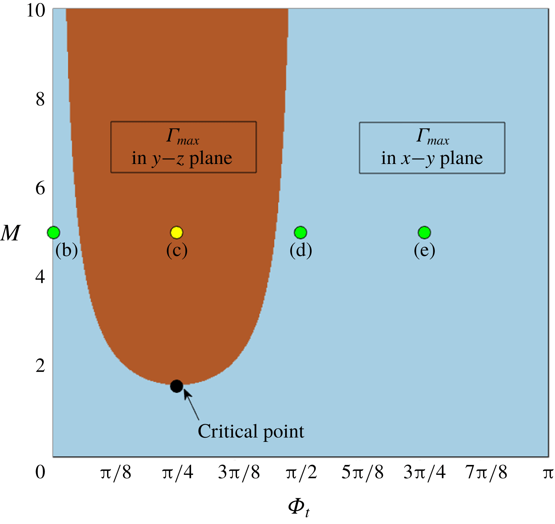
Phase diagram for the location of the peak surfactant concentration
 $(\unicode[STIX]{x1D6E4}_{max})$
on the
 $\unicode[STIX]{x1D6F7}_{t}$
–
 $M$
plane. Here parameters are same as in figure 2. The points (b)–(e) on the phase diagram correspond to the specific parametric states of figures 2(b) to 2(e).

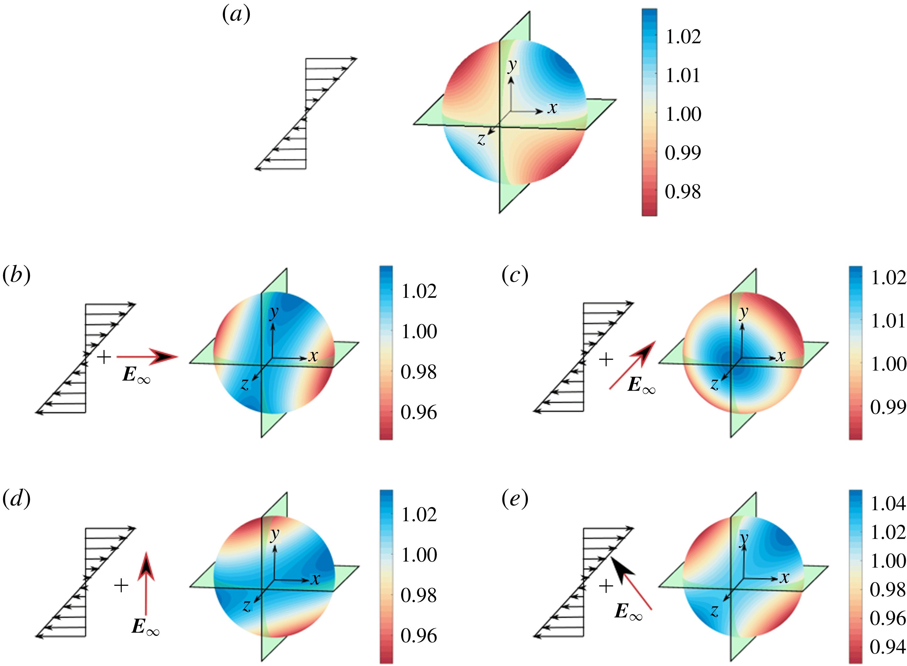
In the absence of any electric field, when only a linear shear flow is imposed, the surfactant molecules obtain a non-uniform but antisymmetric distribution
 $(\unicode[STIX]{x1D6E4}(\unicode[STIX]{x1D703},\unicode[STIX]{x1D719}))$
as shown in figure 2(a). Distribution
 $\unicode[STIX]{x1D6E4}(\unicode[STIX]{x1D703},\unicode[STIX]{x1D719})$
follows the straining axis of the flow which is inclined at an angle
 $\unicode[STIX]{x1D719}=\unicode[STIX]{x03C0}/4$
to the background flow direction (Bentley & Leal Reference Bentley and Leal1986). In that case, the surfactant molecules are observed to accumulate more towards the polar regions of this axis and a dominant depletion takes place orthogonal to these locations. However, this antisymmetric pattern changes when an electric field is applied (shown in figure 2
b–e). With the application of an external field the surfactant distribution does not follow the axisymmetric deposition along
 $\unicode[STIX]{x1D719}=\unicode[STIX]{x03C0}/4$
. While for the tilt angles
 $\unicode[STIX]{x1D6F7}_{t}=0,\unicode[STIX]{x03C0}/2$
and
 $3\unicode[STIX]{x03C0}/4$
this common trend is followed, a completely different characteristic of surfactant distribution emerges for
 $\unicode[STIX]{x1D6F7}_{t}=\unicode[STIX]{x03C0}/4$
. In this case the maximum surfactant concentration points are no longer in the plane of shear (
 $x$
–
 $y$
plane in this case) and the maximum points shift to the
 $y$
–
 $z$
plane which is orthogonal to the plane of shear. A comprehensive picture of the critical tilt angle of the applied electric field for the maxima shift of surfactant distribution can be obtained from the phase map shown in figure 3. It shows that along with the tilt angle, the Mason number (
 $M$
), indicating the relative importance of the electrical stress in comparison to the hydrodynamic stress, also strongly influences the surfactant distribution along the interface, thereby modulating the location of
 $\unicode[STIX]{x1D6E4}_{max}$
. Until a critical Mason number of
 $M\approx 1.56$
(for this specific set of parameters) is reached the maximum lies in the
 $x$
–
 $y$
plane for any value of the tilt angle. However, beyond this critical point, there exists an intermediate regime of tilt angles, for which the maximum of surfactant concentration shifts to the
 $y$
–
 $z$
plane, while for the rest of the tilt angles the maximum appears in the plane of shear (
 $x$
–
 $y$
plane). The range of this band of intermediate tilt angles widens gradually with increasing Mason number. It has been found that surfactant characterization parameters
 $\unicode[STIX]{x1D6FD}$
and
 $k$
have negligible effect on the maxima shift. This can be further confirmed by observing figure S-1(a,c), which shows the dependence of the maxima value on both
 $\unicode[STIX]{x1D6FD}$
and
 $k$
, although the angular positions of the peaks remain unaltered.
Undulations in the local surfactant concentration trigger corresponding changes in the interfacial tension
 $\unicode[STIX]{x1D6FE}(\unicode[STIX]{x1D703},\unicode[STIX]{x1D719})$
and gradients in surface tension
 $(|\unicode[STIX]{x1D6FE}_{max}-\unicode[STIX]{x1D6FE}_{min}|)$
along the drop surface. This influence of Mason number
 $(M)$
on the surface tension is described in figure S-2 for the configuration of a vertically applied electric field. It shows that the symmetric deviation of the maximum and minimum surface tension about the equilibrium condition, in the case of simple shear flow, is not maintained when an electric field is applied. Also, the gradients in surface tension
 $(|\unicode[STIX]{x1D6FE}_{max}-\unicode[STIX]{x1D6FE}_{min}|)$
become progressively higher as the influence of electrical stresses increases relative to their hydrodynamic counterparts.
The above characteristics of
 $\unicode[STIX]{x1D6E4}(\unicode[STIX]{x1D703},\unicode[STIX]{x1D719})$
under different conditions become clear by consideration of (A 2). It shows that different modes in
 $\unicode[STIX]{x1D6E4}^{(Ca)}$
contain the information of various aspects governing the flow physics. While
 $\unicode[STIX]{x1D6E4}_{2,0}^{(Ca)}$
and
 $\unicode[STIX]{x1D6E4}_{2,2}^{(Ca)}$
are only present when an external electric field is applied, the harmonic
 $\hat{\unicode[STIX]{x1D6E4}}_{2,2}^{(Ca)}$
has a non-zero component arising solely from hydrodynamic origin. Again, the surfactant harmonics are strongly dependent on the tilt angle of the applied electric field. Harmonic
 $\unicode[STIX]{x1D6E4}_{2,0}^{(Ca)}$
appears for any configuration of the electric field, but
 $\unicode[STIX]{x1D6E4}_{2,2}^{(Ca)}$
vanishes completely when the tilt angle becomes
 $\unicode[STIX]{x1D6F7}_{t}=\unicode[STIX]{x03C0}/4$
or
 $3\unicode[STIX]{x03C0}/4$
. Similarly, the electric component of
 $\hat{\unicode[STIX]{x1D6E4}}_{2,2}^{(Ca)}$
becomes zero when the electric field is applied in either horizontal
 $(\unicode[STIX]{x1D6F7}_{t}=0)$
or vertical
 $(\unicode[STIX]{x1D6F7}_{t}=\unicode[STIX]{x03C0}/2)$
configuration. In order to investigate the physics behind the coupled behaviour of imposed linear shear and electric field, we appeal to the flow characteristics around the drop originating from the individual effects, as identified in earlier studies (Vlahovska Reference Vlahovska2011; Mandal & Chakraborty Reference Mandal and Chakraborty2017b
). The linear shear flow can be decomposed as a combination of a pure straining and pure rotational flow. On the other hand, the externally applied tilted electric field can give rise to either a uniaxial (for
 $R>S$
) or biaxial (for
 $R<S$
) straining flow around the drop. Hence, under the simultaneous action of shear flow and electrically induced flow, the surfactant molecules assume diverse redistribution patterns, the final form of which is determined by a combined interfacial convection and diffusive transport.
4.2 Leading-order bulk rheology
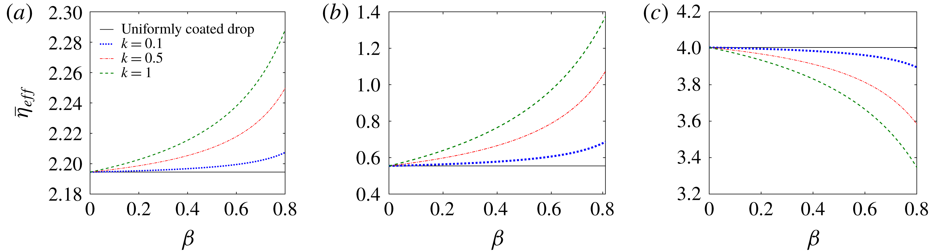
Leading-order normalized effective shear viscosity
 $\bar{\unicode[STIX]{x1D702}}_{eff}=(\unicode[STIX]{x1D702}_{eff}^{(0)}-1)/\unicode[STIX]{x1D708}$
versus elasticity parameter for different physicochemical constants,
 $k$
. The electrohydrodynamic parameters correspond to (a) system-A, (b) system-B and (c) system-C. A Mason number of
 $M=2$
is chosen.

In figure 4(a–c), the contribution of non-uniform surfactant distribution on the drop surface, in modulating the leading-order normalized effective shear viscosity
 $(\bar{\unicode[STIX]{x1D702}}_{eff}^{(0)}=(\unicode[STIX]{x1D702}_{eff}^{(0)}-1)/\unicode[STIX]{x1D708})$
, is described. It is observed from figure 4(a,b) that an increase in either of the parameters
 $\unicode[STIX]{x1D6FD}$
or
 $k$
causes an enhancement in the effective viscosity. In contrast, figure 4(c) depicts that the surfactant characterization parameters have a completely reverse effect on
 $\bar{\unicode[STIX]{x1D702}}_{eff}$
. To understand the effects of the surfactant characterization parameters
 $\unicode[STIX]{x1D6FD}$
and
 $k$
, we appeal to figure S-1 (see Supplementary_2 of the supplementary material) where the variations in surfactant concentration and surface tension are shown. The surface elasticity number,
 $\unicode[STIX]{x1D6FD}$
, signifies the sensitivity of the surface tension to the local surfactant concentration. From figure S-1(a,b), we observe that an increase in
 $\unicode[STIX]{x1D6FD}$
results in an enhanced gradient in surface tension
 $(|\unicode[STIX]{x1D6FE}_{max}-\unicode[STIX]{x1D6FE}_{min}|)$
, but the deviations in the surfactant concentration from the equilibrium condition
 $(|\unicode[STIX]{x1D6E4}_{max}-\unicode[STIX]{x1D6E4}_{min}|)$
become suppressed with increasing
 $\unicode[STIX]{x1D6FD}$
. This behaviour is consistent with the results of Li & Pozrikidis (Reference Li and Pozrikidis1997), where surfactant effects were analysed for the case of a drop in simple shear flow. Greater magnitude of surface tension gradient leads to an enhancement in Marangoni convection which in turn opposes the convective transport of the surfactant. As a result, the distribution of
 $\unicode[STIX]{x1D6E4}$
approaches equilibrium. An increase in
 $k$
, on the other hand, signifies a corresponding increase in the convective transport mechanism of the surfactants (see (3.7)). Thus, for a fixed
 $\unicode[STIX]{x1D6FD}$
, when
 $k$
is increased, the convective transport of surfactants dominates over the effect due to increased surface tension gradient, resulting in greater undulations in both
 $\unicode[STIX]{x1D6E4}$
and
 $\unicode[STIX]{x1D6FE}$
from the equilibrium condition as portrayed in supplementary figures S-1(c) and S-1(d), respectively. The Marangoni effect due to non-uniformity in surfactant distribution modifies the balance between the tangential component of the hydrodynamic and electrical Maxwell stresses at the interface (see (3.6a,b
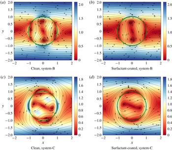
)). In order to visualize the effect of surfactant coating on the drop surface, in figure 5 we demonstrate the flow fields for some representative cases. This figure shows that the orientation of the vorticity poles for system-B (figure 5
a,b) is vertical while it becomes horizontal for system-C (figure 5
c,d). The surfactants create further alterations in both the velocity magnitude and the pattern of the disturbance flow around the drop. This subsequently causes an enhancement or reduction in the viscous dissipation of the bulk mixture and finally a corresponding change in the effective viscosity results.
Comparison of leading-order flow fields in and around a drop for clean and surfactant-coated cases. The streamlines are shown in the plane of shear and with respect to a body-fitted reference frame. The colourbars show the variation in velocity magnitude, while the green circle in each panel denotes the drop–matrix interface. (a,b) System-B,
 $M=5$
; (c,d) system-C,
 $M=5$
. The parameters are chosen as
 $\unicode[STIX]{x1D6F7}_{t}=\unicode[STIX]{x03C0}/4,\unicode[STIX]{x1D6FD}=0.8$
and
 $k=1$
.

The dependence of the normalized effective shear viscosity
 $(\bar{\unicode[STIX]{x1D702}}_{eff}=(\unicode[STIX]{x1D702}_{eff}^{(0)}-1)/\unicode[STIX]{x1D708})$
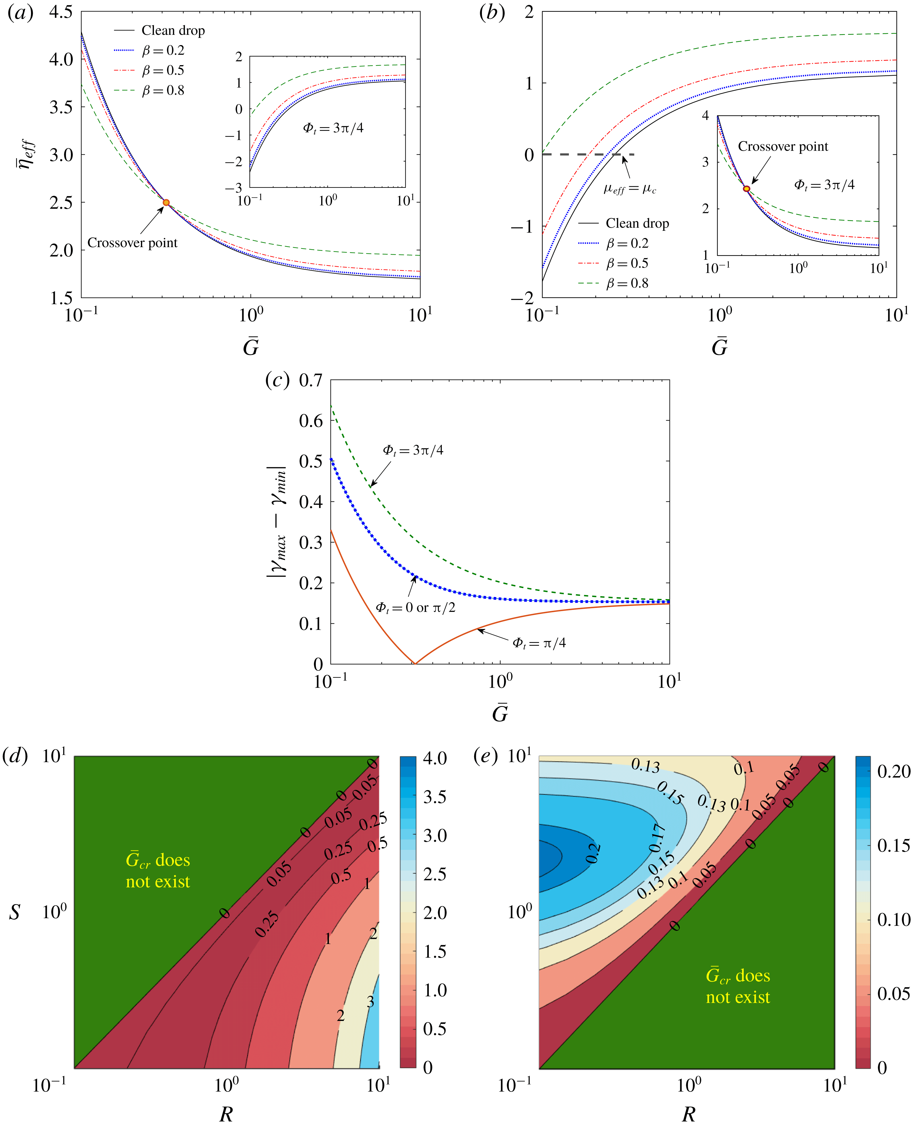
on the shear rate is shown in figure 6(a,b) for two different combinations of electrohydrodynamic parameters. First, we define a relative hydrodynamic shear rate with respect to the electrical stress as
 $\bar{G}=1/M=\unicode[STIX]{x1D707}_{c}\widetilde{G}/\unicode[STIX]{x1D716}_{c}\widetilde{E}_{\infty }^{2}$
. It was previously reported (Mandal & Chakraborty Reference Mandal and Chakraborty2017b
) that in the leading order, the effective viscosity becomes a function of relative shear rate
 $\bar{G}$
only when the electric field is tilted with respect to the direction of the applied shear flow, while the emulsion shows a Newtonian behaviour when the electric field is applied along either the direction of shear flow or its gradient. A careful inspection of these figures reveals that the non-uniformity surfactant distribution has a potential in altering the non-Newtonian shear rate dependency of the effective shear rate. It is quite interesting to find from figure 6(a) that for a tilt angle of external electric field
 $\unicode[STIX]{x1D6F7}_{t}=\unicode[STIX]{x03C0}/4$
, there exists a crossover point at
 $\bar{G}\sim 0.2$
before which an increase in
 $\unicode[STIX]{x1D6FD}$
causes the effective shear viscosity to decrease in comparison to an uncontaminated drop, while beyond this point a corresponding increase in
 $\bar{\unicode[STIX]{x1D702}}_{eff}$
results with similar changes in
 $\unicode[STIX]{x1D6FD}$
. However, for
 $\unicode[STIX]{x1D6F7}_{t}=3\unicode[STIX]{x03C0}/4$
,
 $\bar{\unicode[STIX]{x1D702}}_{eff}$
shows a steady enhancement with
 $\unicode[STIX]{x1D6FD}$
. In this case, for a fixed relative shear rate, the variation in
 $\unicode[STIX]{x1D6FD}$
can lead to a change in effective shear viscosity to such an extent that it becomes greater than the viscosity of the continuous medium
 $\bar{\unicode[STIX]{x1D702}}_{eff}>0$
, or
 $\unicode[STIX]{x1D707}_{eff}>\unicode[STIX]{x1D707}_{c}$
, becoming increased from a condition of
 $\bar{\unicode[STIX]{x1D702}}_{eff}<0$
, or
 $\unicode[STIX]{x1D707}_{eff}<\unicode[STIX]{x1D707}_{c}$
, for a clean drop. The role of the electric field tilt angle is reversed for system-B, as shown in figure 6(b).
In the electrohydrodynamics literature, the flow behaviour is often shown to be of opposite nature when the electrical property combinations give rise to a positive (
 $R>S$
) or negative (
 $R<S$
) polarity (Taylor Reference Taylor1966; Tsukada et al.
Reference Tsukada, Katayama, Ito and Hozawa1993; Salipante & Vlahovska Reference Salipante and Vlahovska2010; Mandal & Chakraborty Reference Mandal and Chakraborty2017b
). Based on the polarity, the direction of the electrical traction at the interface is altered. However, comparing the present results in figure 4 for different electrohydrodynamic systems, it is observed that the consequence of the Marangoni effect cannot be simply categorized based on the condition of
 $R>S$
or
 $R<S$
. Although system-A and system-B have properties
 $R<S$
and
 $R>S$
, respectively, they exhibit a similar trend of Marangoni effect, while both system-A and system-C show opposite behaviour despite having the same polarity. Along similar lines, in figure 6(a,b), the Marangoni effect is observed to be dependent on the electric field tilt angle (
 $\unicode[STIX]{x1D6F7}_{t}$
) as well. Inspired by such observations, we analyse the expression of the leading-order effective shear viscosity
 $\unicode[STIX]{x1D702}_{eff}^{(0)}$
in (3.14). We obtain a unique discriminating factor in terms of the crossover relative shear rate
 $\bar{G}_{cr}$
given as
 $$\begin{eqnarray}\bar{G}_{cr}^{(0)}=\frac{9}{5}\,\frac{\sin (2\unicode[STIX]{x1D6F7}_{t})(S-R)}{(R+2)^{2}}.\end{eqnarray}$$
Similar discriminating factors have been previously obtained by others in the context of drop deformation (Taylor Reference Taylor1966) and surface charge convection (Xu & Homsy Reference Xu and Homsy2006). If
 $\unicode[STIX]{x1D6F7}_{t}<\unicode[STIX]{x03C0}/2$
then
 $\sin (2\unicode[STIX]{x1D6F7}_{t})$
is a positive quantity. Thus, for a realistic
 $\bar{G}_{cr}^{(0)}$
to exist, the condition which must be satisfied is
 $R<S$
. Again, for
 $\unicode[STIX]{x1D6F7}_{t}>\unicode[STIX]{x03C0}/2$
the property ratios must fulfil the condition
 $R>S$
. Hence, the Marangoni effect on the electrically induced emulsion viscosity can be suitably controlled by finely tuning the combination of the electric field direction and electrical properties of the drop–surrounding fluid pair. To understand such a behaviour of the Marangoni effect, we plot the surface tension gradient
 $(|\unicode[STIX]{x1D6FE}_{max}-\unicode[STIX]{x1D6FE}_{min}|)$
with relative shear rate for different values of the tilt angle in figure 6(c) for system-A. It shows that the surface tension gradient vanishes at a relative shear rate which is exactly equal to the crossover point observed in figure 6(a). This indicates that due to competitive effects of the hydrodynamic and electrical stresses on the surface tension variation, for a specific relative shear rate, the Marangoni effect vanishes completely and the drop surface behaves as an uncontaminated one. The corresponding competing effects can be realized by referring back to (3.14) where distinct functional forms of the hydrodynamic and electric surfactant contribution terms
 $(\unicode[STIX]{x1D702}_{h,surf}^{(0)},\unicode[STIX]{x1D702}_{e,surf}^{(0)})$
appeared in the expression of
 $\unicode[STIX]{x1D702}_{eff}^{(0)}$
. The lesser extent of variation of
 $\unicode[STIX]{x1D702}_{eff}^{(0)}$
with
 $\bar{G}$
, after the crossover point
 $\bar{G}_{cr}$
is reached (observation from figure 6
a), can also be explained from figure 6(c) where the range of surface tension gradient
 $(|\unicode[STIX]{x1D6FE}_{max}-\unicode[STIX]{x1D6FE}_{min}|)$
becomes lower after
 $\bar{G}_{cr}$
than it was before
 $\bar{G}_{cr}$
.
The value range of
 $\bar{G}_{cr}^{(0)}$
is observed to be different in the two sets of electrohydrodynamic parameters. In this context, the parametric mapping of the critical relative shear rate on the
 $R$
–
 $S$
plane is shown for two different tilt angles in figure 6(d,e). It is to be noted that a critical normalized shear rate was obtained previously by Mandal & Chakraborty (Reference Mandal and Chakraborty2017b
) in relation to a surfactant-free drop under the combined influence of electric field and shear flow. In that case, the critical parameter had been used to characterize whether the effective shear viscosity is greater (or lesser) than that of the suspending medium. In stark contrast, the presently obtained critical relative shear rate is related to the surfactant-induced Marangoni effect. To the best of our knowledge, for the first time we have obtained a discriminating factor in terms of a relative shear rate for which the Marangoni effect will have no contribution in altering the emulsion rheology.
Variation of normalized effective shear viscosity
 $(\bar{\unicode[STIX]{x1D702}}_{eff})$
with relative shear rate
 $\bar{G}=1/M$
for different values of the elasticity parameter,
 $\unicode[STIX]{x1D6FD}$
: (a) system-A and (b) system-B. In both panels,
 $\unicode[STIX]{x1D6F7}_{t}=\unicode[STIX]{x03C0}/4$
is chosen, while the inset of each panel shows the corresponding variations for
 $\unicode[STIX]{x1D6F7}_{t}=3\unicode[STIX]{x03C0}/4$
. (c) Variation of surface tension gradient
 $(|\unicode[STIX]{x1D6FE}_{max}-\unicode[STIX]{x1D6FE}_{min}|)$
with relative shear rate for various
 $\unicode[STIX]{x1D6F7}_{t}$
. Here the demonstration is for system-A. Maps of the critical relative shear rate on the
 $(R,S)$
plane for electric field tilt angle (d)
 $\unicode[STIX]{x1D6F7}_{t}=\unicode[STIX]{x03C0}/4$
and (e)
 $\unicode[STIX]{x1D6F7}_{t}=3\unicode[STIX]{x03C0}/4$
.

Another important aspect of bulk rheology, i.e. the first
 $(N_{1}^{(0)})$
and second
 $(N_{2}^{((0))})$
normal stress difference, is significantly affected by the presence of surfactant contamination on the drop surface. Equation (3.15) shows that in the leading order, the normal stress differences in the bulk rheology arise only from electrohydrodynamic origins, even when the surfactant effects are considered. From the functional form of
 ${\mathcal{N}}_{surf}^{(0)}$
, it is evident that for all the realistic parametric ranges of (
 $0\leqslant \unicode[STIX]{x1D6FD}<1,k>0$
and
 $\unicode[STIX]{x1D706}>0$
), the surfactant-induced Marangoni effect always acts to reduce the normal stress differences, i.e.
 ${\mathcal{N}}_{surf}^{(0)}<1$
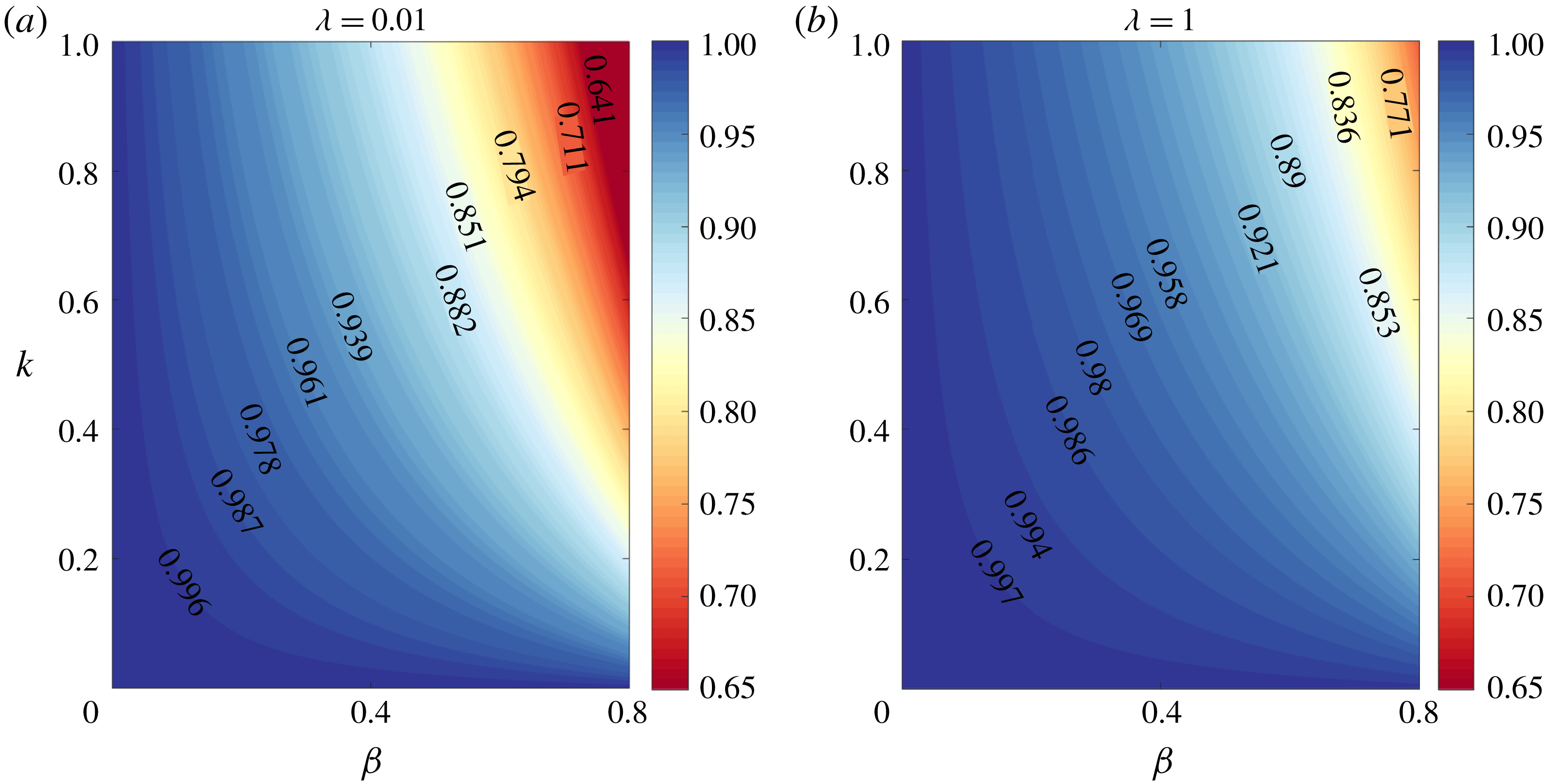
. In figure 7, a parametric map of the common surfactant contribution factor
 ${\mathcal{N}}_{surf}^{(0)}$
(defined in (3.16)) is shown on the
 $\unicode[STIX]{x1D6FD}$
–
 $k$
plane for different viscosity ratios of the drop–matrix fluid pair. It shows that for lower viscosity of the drop phase as compared to the matrix fluid, the surfactant contribution is more prominently observed. In the limit of
 $\unicode[STIX]{x1D706}\rightarrow 0$
, when the drop tends behave as a bubble, the surfactant effect is a maximum and we obtain
 $\lim _{\unicode[STIX]{x1D706}\rightarrow 0}\,{\mathcal{N}}_{surf}^{(0)}=(1-\unicode[STIX]{x1D6FD})/((k-5)\unicode[STIX]{x1D6FD}+5)$
. In the other limit of
 $\unicode[STIX]{x1D706}\rightarrow \infty$
, the drop behaves like a particle and its surface becomes completely immobilized. In that case, the normal stress differences vanish for a spherical drop.
Surfactant modification parameter for the normal stress differences of the emulsion
 $({\mathcal{N}}^{(0)})$
on
 $\unicode[STIX]{x1D6FD}$
–
 $k$
plane for different viscosity ratios (
 $\unicode[STIX]{x1D706}$
).

4.3 Order
 $Re_{E}$
bulk rheology

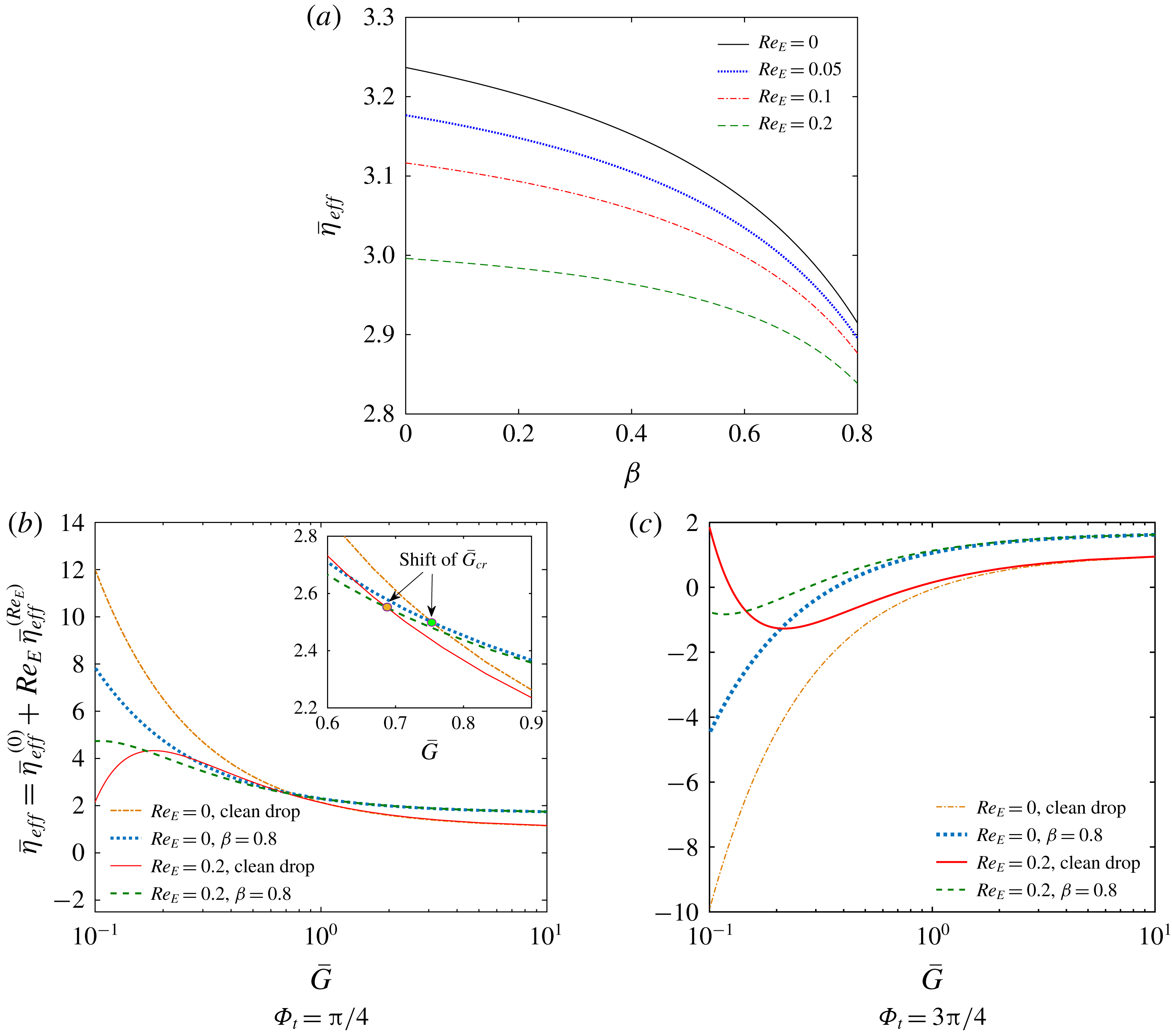
Figure 8(a) depicts that an increase in the parameter
 $\unicode[STIX]{x1D6FD}$
suppresses the
 $O(Re_{E})$
modifications in
 $\bar{\unicode[STIX]{x1D702}}_{eff}$
. To justify such a phenomenon, we plot the variations in
 $O(Re_{E})$
surface velocity and the electrical traction at the interface in figure S-4 for different values of
 $\unicode[STIX]{x1D6FD}$
. The figure shows that the charge-convection-induced modifications in the flow characteristics (exemplified by modulations in
 $u_{S,\unicode[STIX]{x1D719}}^{(Re_{E})}$
and
 $[[T_{\unicode[STIX]{x1D719}}^{E}]]^{(Re_{E})}$
) are severely altered due to the surface elasticity parameter,
 $\unicode[STIX]{x1D6FD}$
.
The interplay between the charge convection and Marangoni flow (see the discussion in § S-5 of Supplementary_2) at the interface also modifies the shear-rate-dependent response of the emulsion viscosity, as shown in figure 8. The critical relative shear rate corresponding to the crossover point of the Marangoni effect,
 $(\bar{G}_{cr})$
, is shifted from its leading-order counterpart (shown in figure 8
a). This effect can be substantiated by carefully inspecting the
 $O(Re_{E})$
effective shear viscosity (
 $\unicode[STIX]{x1D702}_{eff}^{(Re_{E})}$
). Similar to the leading order, there exists a specific range of relative shear rate for which the Marangoni effect has hardly any role in modifying the
 $O(Re_{E})$
effective viscosity of the medium (
 $\unicode[STIX]{x1D702}_{eff}^{(Re_{E})}$
). However, the critical shear rate in this case is also a function of the surfactant parameters and the viscosity ratio:
 $$\begin{eqnarray}\bar{G}_{cr,\bar{\unicode[STIX]{x1D702}}}^{(Re_{E})}=\frac{R-S}{(R+2)^{2}}\frac{\sin (2\unicode[STIX]{x1D6F7}_{t})}{\unicode[STIX]{x1D6FF}_{1}\cos (2\unicode[STIX]{x1D6F7}_{t})+\unicode[STIX]{x1D6FF}_{2}},\end{eqnarray}$$
where
 $$\begin{eqnarray}\unicode[STIX]{x1D6FF}_{1}=\frac{175}{36}\frac{(3R+4)(\unicode[STIX]{x1D706}+1)(R-2S-2)(\unicode[STIX]{x1D6FD}k-5\unicode[STIX]{x1D6FD}\unicode[STIX]{x1D706}-5\unicode[STIX]{x1D6FD}+5\unicode[STIX]{x1D706}+5)}{(69R^{2}-54RS+130R-80S+40)(\unicode[STIX]{x1D6FD}k-10\unicode[STIX]{x1D6FD}\unicode[STIX]{x1D706}-10\unicode[STIX]{x1D6FD}+10\unicode[STIX]{x1D706}+10)}\end{eqnarray}$$
and
 $$\begin{eqnarray}\unicode[STIX]{x1D6FF}_{2}=-\frac{5}{108}\frac{(701\,R^{2}-506\,RS+1410\,R-760\,S+520)}{(69\,R^{2}-54\,RS+130\,R-80\,S+40)}.\end{eqnarray}$$
In addition, comparing figures 8(a) and 8(b), we observe that the non-Newtonian shear-thickening (shear-thinning) rheology at low shear rates (corresponding to the curve
 $Re_{E}=0.2,$
clean drop) becomes a shear-thinning (shear-thickening) one in the presence of surfactant (refer to the curve
 $Re_{E}=0.2,\unicode[STIX]{x1D6FD}=0.8$
). This reversal in non-Newtonian behaviour is absent when charge convection effects are insignificant.
(a) Normalized effective shear viscosity (
 $\bar{\unicode[STIX]{x1D702}}_{eff}=\bar{\unicode[STIX]{x1D702}}_{eff}^{(0)}+Re_{E}\,\bar{\unicode[STIX]{x1D702}}_{eff}^{(Re_{E})}$
) variation with elasticity parameter
 $\unicode[STIX]{x1D6FD}$
for different electric Reynolds numbers. Here
 $M=2$
and
 $\unicode[STIX]{x1D6F7}_{t}=\unicode[STIX]{x03C0}/4$
. (b,c) Variation of
 $\bar{\unicode[STIX]{x1D702}}_{eff}$
with relative shear rate
 $(\bar{G})$
for different elasticity parameters
 $\unicode[STIX]{x1D6FD}$
and electric Reynolds number
 $Re_{E}$
. In the inset of (b), the shift of critical shear rate
 $\bar{G}_{cr}$
with
 $Re_{E}$
is highlighted. Here
 $\unicode[STIX]{x1D6F7}_{t}=\unicode[STIX]{x03C0}/4$
and
 $\unicode[STIX]{x1D6F7}_{t}=3\unicode[STIX]{x03C0}/4$
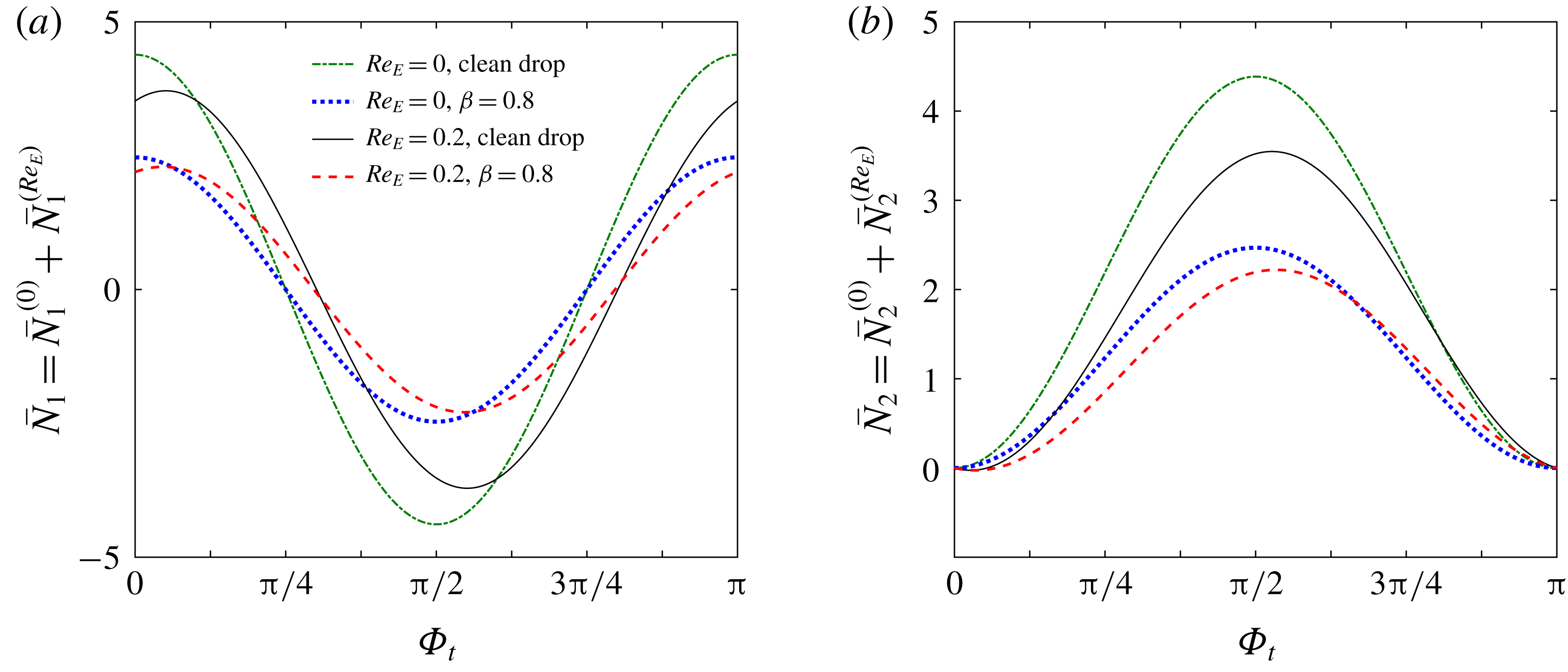
in panels (b) and (c), respectively. The other parameters in all panels are chosen following system-C.

In the absence of charge convection, the surfactant contributions to the first and second normal stress differences
 $(\unicode[STIX]{x0394}\bar{N}_{1}=|\bar{N}_{1}-\bar{N}_{1,clean}|,\unicode[STIX]{x0394}\bar{N}_{2}=|\bar{N}_{2}-\bar{N}_{2,clean}|)$
increase with the tilt angle and are symmetric about
 $\unicode[STIX]{x1D6F7}_{t}=\unicode[STIX]{x03C0}/2$
, as depicted in figure 9. The value of
 $\unicode[STIX]{x0394}\bar{N}_{1}$
is a maximum for
 $\unicode[STIX]{x1D6F7}_{t}=0,\unicode[STIX]{x03C0}/2$
and vanishes for
 $\unicode[STIX]{x1D6F7}_{t}=\unicode[STIX]{x03C0}/4$
; while
 $\unicode[STIX]{x0394}\bar{N}_{1}$
increases from zero to maximum from
 $\unicode[STIX]{x1D6F7}_{t}=0$
to
 $\unicode[STIX]{x03C0}/2$
. However, owing to the presence of charge convection, such symmetric nature is broken, although the increasing trends of both
 $\unicode[STIX]{x0394}\bar{N}_{1}$
and
 $\unicode[STIX]{x0394}\bar{N}_{2}$
are preserved.
Variation of normalized (a) first
 $(\bar{N}_{1}=N_{1}/\unicode[STIX]{x1D708})$
and (b) second
 $(\bar{N}_{2}=N_{2}/\unicode[STIX]{x1D708})$
normal stress differences with the tilt angle of the applied electric field
 $\unicode[STIX]{x1D6F7}_{t}$
for different values of elasticity parameter
 $\unicode[STIX]{x1D6FD}$
and electrical Reynolds number
 $Re_{E}$
. Here the electrohydrodynamic parameters are chosen according to system-C. Other parameters are
 $M=2$
and
 $k=1$
.

4.4 Bulk rheology of deformed drops
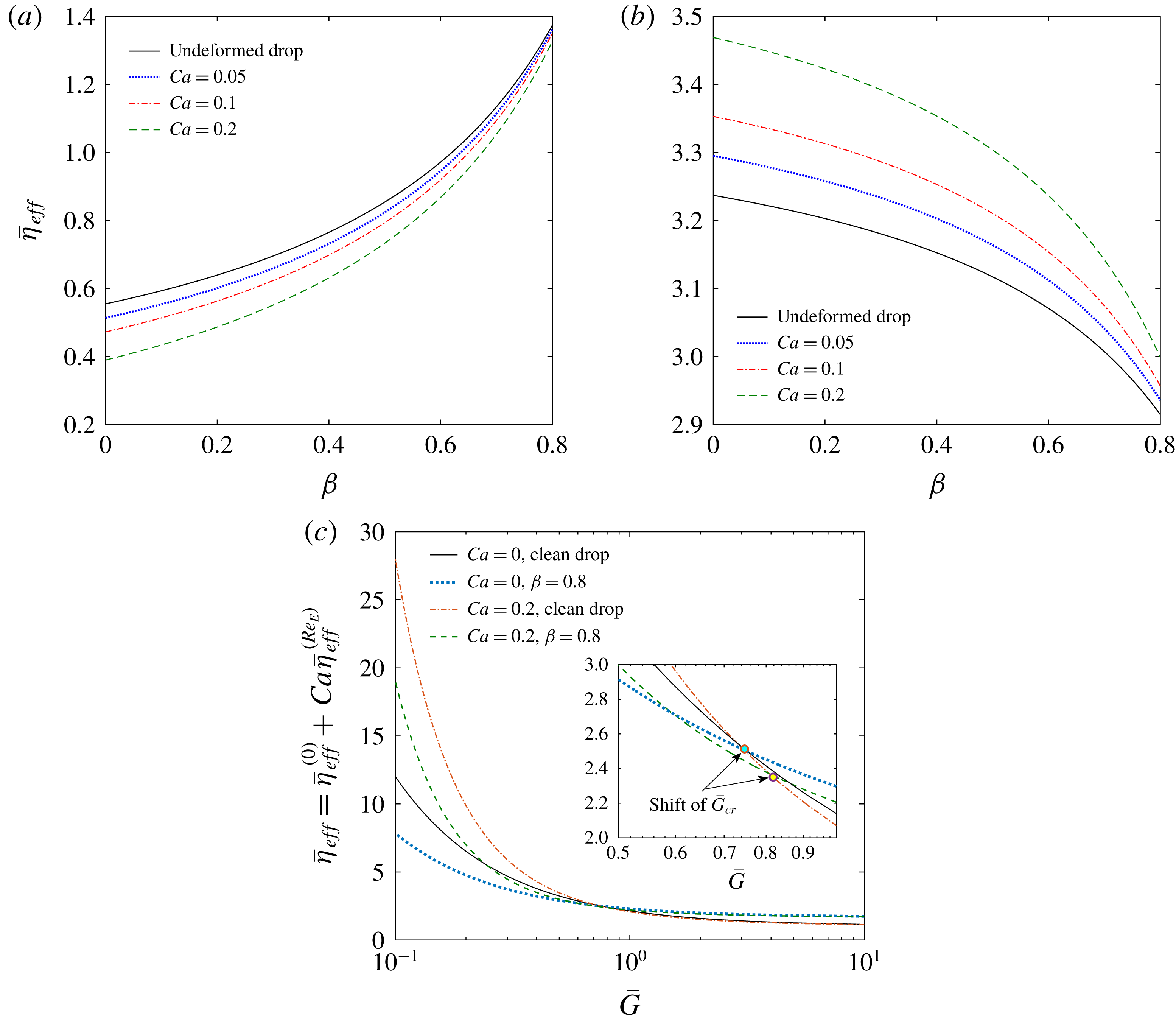
Here, we analyse the consequences of the coupled interaction between the deformable nature of the drop and surfactant coating for different electrohydrodynamic systems. From figure 10(a,b), it can be observed that the deformation-induced modification in the Marangoni effect is much pronounced for lower values of the elasticity parameter
 $\unicode[STIX]{x1D6FD}$
. Also, the effect of capillary number becomes diminished as
 $\unicode[STIX]{x1D6FD}\rightarrow 0.8.$
Most interestingly, the increase in capillary number causes a decrease in the effective viscosity for system-B, whereas the trend is opposite for system-C.
To understand the physical origin of such behaviour, we investigate the nature of drop deformation in different systems and the consequence of surfactant coating on the drops. For this, we appeal to the stress balance equation (3.6a,b
) where the Marangoni effect is seen to play its role. From a physical perspective, the localized accumulation of surfactant molecules reduces the local surface tension and makes that region more prone to deformation in order to balance the normal stresses. This is known as the ‘tip stretching’ phenomenon in the literature (Pawar & Stebe Reference Pawar and Stebe1996). Again, due to increased surface area of the deformed drop, the overall surfactant concentration gets diluted and the local surface tension tends to decrease. The electrical contribution to the deformation of a surfactant-free drop surface is further modified by surface contamination and the deformation parameter shows a steady increase with
 $\unicode[STIX]{x1D6FD}$
as shown in figures S-5(a,b). This leads to modifications in the nature as well as the intensity of drop deformation. As a result, the drop poses different kinds of resistances to the imposed shear flow, thereby creating diverse modulations in the effective shear viscosity of the emulsion.
Normalized effective shear viscosity (
 $\bar{\unicode[STIX]{x1D702}}_{eff}=\bar{\unicode[STIX]{x1D702}}_{eff}^{(0)}+Ca\,\bar{\unicode[STIX]{x1D702}}_{eff}^{(Ca)}$
) versus elasticity parameter
 $\unicode[STIX]{x1D6FD}$
for different capillary numbers
 $Ca$
: (a) system-B and (b) system-C. Here
 $M=2$
. (c) Normalized effective shear viscosity versus relative shear rate for different elasticity parameter
 $\unicode[STIX]{x1D6FD}$
and capillary number
 $Ca$
. In the inset, the shift of critical shear rate
 $\bar{G}_{cr}$
with
 $Ca$
is highlighted. Here, other parameters are chosen following system-C. In all panels,
 $\unicode[STIX]{x1D6F7}_{t}=\unicode[STIX]{x03C0}/4$
and
 $k=1$
.

Figure 10(c) shows that the critical shear rate corresponding to the vanishing Marangoni effect
 $(\bar{G}_{cr})$
is shifted to a higher value when the capillary number becomes 0.2 from an undeformed state, for the specific parametric choices of system-C. Until
 $\bar{G}_{cr}$
is reached, the shape deformation causes significant enhancement in the effective shear viscosity. However, with an increase in
 $\bar{G}$
beyond this critical point, the impact of deformation effects on the effective viscosity becomes vanishingly small.
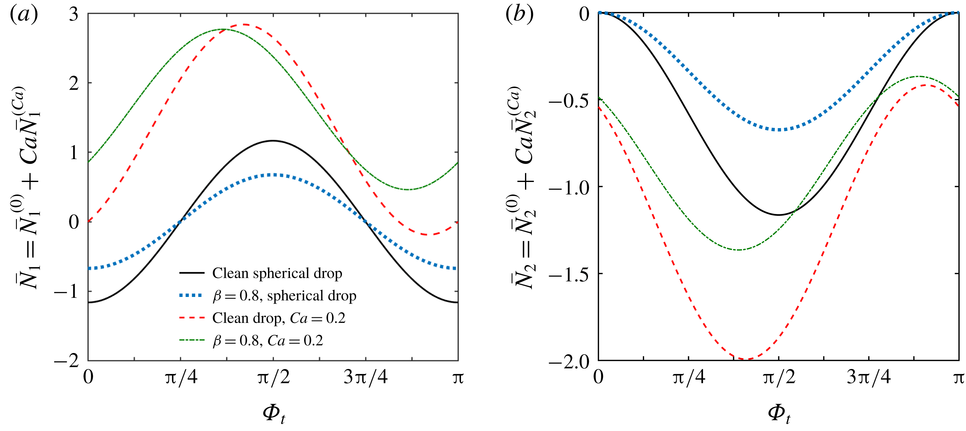
In figure 11, we demonstrate the variations in the bulk normal stress differences with the tilt angle of the applied electric field for different values of the surface elasticity number and capillary number. It is found that the leading-order symmetry in both
 $\bar{N}_{1}$
and
 $\bar{N}_{2}$
about the tilt angle
 $\unicode[STIX]{x1D6F7}_{t}=\unicode[STIX]{x03C0}/2$
is destroyed, owing to a deformed drop surface. In the deformed condition, the contribution of the surfactants in modifying the first normal stress difference
 $(\unicode[STIX]{x0394}\bar{N}_{1}=|\bar{N}_{1}-\bar{N}_{1,clean}|)$
is observed to be positive for certain values of the tilt angle, while the reverse happens for other tilt angles (shown in figure 11
a). However, figure 11(b) depicts that under similar circumstances, the surfactant-induced modifications in the second normal stress difference
 $(\unicode[STIX]{x0394}\bar{N}_{2}=|\bar{N}_{2}-\bar{N}_{2,clean}|)$
show a steady decrease for all the tilt angles between
 $\unicode[STIX]{x1D6F7}_{t}=0$
and
 $\unicode[STIX]{x03C0}$
. Variations in the orientation of the applied electric field not only alter the behaviour of the drop deformation but also cause severe changes in the electrohydrodynamic flow pattern around the drop. In turn, the surface tension gradient is redistributed. Finally, an intricate interplay between the physical mechanisms of electrohydrodynamic and Marangoni flow dictates the elastic characteristics of the emulsion, resulting in corresponding changes in the normal stress differences.
Normalized (a) first
 $(\bar{N}_{1}=N_{1}/\unicode[STIX]{x1D708})$
and (b) second
 $(\bar{N}_{2}=N_{2}/\unicode[STIX]{x1D708})$
normal stress differences versus tilt angle of the applied electric field
 $\unicode[STIX]{x1D6F7}_{t}$
for various elasticity parameter
 $\unicode[STIX]{x1D6FD}$
and capillary number
 $Ca$
. Here the electrohydrodynamic parameters are chosen according to system-B. Other parameters are
 $M=2$
and
 $k=1$
.

5 Conclusions
We have presented a detailed analysis of the surfactant coating effects on the electrorheology of a dilute emulsion. We have considered a linear shear flow and tilted electric field acting in tandem on a deformable viscous drop which is covered with a non-ionic, bulk insoluble surfactant. The charge convection phenomena and interfacial surfactant transport affect each other in a strongly coupled manner, and subsequently the nature of viscous dissipation due to the presence of the drops becomes altered. This is reflected through the corresponding non-trivial alterations in the bulk emulsion rheology.
Our main results indicate a complex interplay among hydrodynamic, electrical and Marangoni stresses which is manifested through a unique shift of the location of peak surfactant accumulation from the plane of shear to a plane orthogonal to it. The relative intensity of the hydrodynamic and electrical stresses, quantified by the Mason number, determines the points of peak surfactant accumulation and, in turn, the effect of surface tension gradient
 $(|\unicode[STIX]{x1D6FE}_{max}-\unicode[STIX]{x1D6FE}_{min}|)$
on the interface is also influenced. We also report the unique existence of a critical hydrodynamic shear rate relative to the electric stress for which the surface tension gradient vanishes on the drop surface. At this critical relative shear rate, the corresponding surfactant effect on the effective shear viscosity vanishes. This critical shear rate strongly depends on the tilt angle of the applied electric field, the electrical conductivity ratio and the permittivity ratio of the drop–matrix pair.
Additionally, we have found that the bulk normal stress differences, describing the anisotropy in the normal stress of the effective fluid mixture, always reduce due to the surfactant effect in the leading order. This decrease becomes much pronounced for low drop viscosities.
The drop deformation is found to be also severely influenced by the Marangoni stresses. Not only the bulk shear viscosity, but also the effective tension along the flow streamlines (observable through the modulations in the first and second normal stress difference) is affected by the physical interaction of the electrohydrodynamic and surfactant-induced Marangoni stresses.
To summarize, the detailed analysis presented in this work shows that the perturbation in drop-scale flow dynamics, created due to the presence of dispersed drops under the combined action of shear flow and uniform electric field, can be severely modulated by surfactant coating at the interface. We have explored diverse parametric regimes where the crucial shifts in the surfactant distribution and surface stress take place. Such understanding of the interfacial-scale flow physics thus becomes a stepping stone towards analysing more complex rheological behaviour of emulsions where multi-drop interactions become inevitable. We envisage that experimental difficulties may arise in obtaining evidence of such critical shear rates and the described effects if the drop significantly deviates from sphericity, the surfactant has the property of being soluble in either of the phases and/or the emulsion contains densely suspended drops. Under many circumstances, higher-order inertial effects may become important including the scenarios of a simple shear flow around a deformable drop (Lin, Peery & Schowalter Reference Lin, Peery and Schowalter1970; Li & Sarkar Reference Li and Sarkar2005) as well as electrohydrodynamics (Lanauze, Walker & Khair Reference Lanauze, Walker and Khair2013; Nganguia et al. Reference Nganguia, Young, Layton, Lai and Hu2016). In such scenarios, the present study can be extended to obtain the possible correction terms in terms of the hydrodynamic Reynolds number. In addition, taking account of the oscillatory shear flow, which is typical in many rheology experiments, may open up a new avenue of research where the possible linear viscoelastic behaviour of the emulsion becomes influenced by coupled interplay of the electrohydrodynamic and Marangoni stresses.
Acknowledgements
S.C. acknowledges the financial support provided by the Department of Science and Technology, Government of India, through the J. C. Bose National Fellowship, for conducting this research.
Supplementary material
The detailed expressions of various parameters, as referred to in the main text, are included in the MATLAB file named ‘Supplementary_1.m’. Also various descriptive plots and discussions are provided in the file named ‘Supplementary_2.pdf’.
Supplementary material is available at https://doi.org/10.1017/jfm.2019.745.
Appendix A. Detailed expression of the
$O(Ca)$
surfactant concentration and leading-order surface velocity

The surfactant distribution up to
 $O(Ca)$
can be expressed as
 $$\begin{eqnarray}\displaystyle \unicode[STIX]{x1D6E4} & = & \displaystyle \unicode[STIX]{x1D6E4}^{(0)}+Ca\,\unicode[STIX]{x1D6E4}^{(Ca)}=\unicode[STIX]{x1D6E4}^{(0)}+Ca\,(\unicode[STIX]{x1D6E4}_{2,0}^{(Ca)}P_{2,0}(\unicode[STIX]{x1D702})+\unicode[STIX]{x1D6E4}_{2,2}^{(Ca)}\cos (2\unicode[STIX]{x1D719})P_{2,2}(\unicode[STIX]{x1D702})\nonumber\\ \displaystyle & & \displaystyle +\,\hat{\unicode[STIX]{x1D6E4}}_{2,2}^{(Ca)}\sin (2\unicode[STIX]{x1D719})P_{2,2}(\unicode[STIX]{x1D702})),\end{eqnarray}$$
where
 $$\begin{eqnarray}\left.\begin{array}{@{}c@{}}\displaystyle \unicode[STIX]{x1D6E4}^{(0)}=1;\\ \displaystyle \unicode[STIX]{x1D6E4}_{2,0}^{(Ca)}=-\frac{3}{2}\frac{M(1-\unicode[STIX]{x1D6FD})(R-S)k}{(R+2)^{2}((k-5\unicode[STIX]{x1D706}-5)\unicode[STIX]{x1D6FD}+5\unicode[STIX]{x1D706}+5)};\\ \displaystyle \unicode[STIX]{x1D6E4}_{2,2}^{(Ca)}=\frac{3}{4}\frac{M\cos (2\unicode[STIX]{x1D6F7}_{t})(1-\unicode[STIX]{x1D6FD})(R-S)k}{(R+2)^{2}((k-5\unicode[STIX]{x1D706}-5)\unicode[STIX]{x1D6FD}+5\unicode[STIX]{x1D706}+5)};\\ \displaystyle \hat{\unicode[STIX]{x1D6E4}}_{2,2}^{(Ca)}=\frac{5}{12}\frac{(1-\unicode[STIX]{x1D6FD})k}{(k-5\unicode[STIX]{x1D706}-5)\unicode[STIX]{x1D6FD}+5\unicode[STIX]{x1D706}+5}+\frac{3}{4}\frac{M\sin (2\unicode[STIX]{x1D6F7}_{t})(1-\unicode[STIX]{x1D6FD})(R-S)k}{(R+2)^{2}((k-5\unicode[STIX]{x1D706}-5)\unicode[STIX]{x1D6FD}+5\unicode[STIX]{x1D706}+5)}.\end{array}\right\}\end{eqnarray}$$
The leading-order surface velocity can be expressed in the spherical coordinate system as
 $\boldsymbol{u}_{S}^{(0)}=u_{S,\unicode[STIX]{x1D703}}^{(0)}\,\boldsymbol{i}_{\unicode[STIX]{x1D703}}+u_{S,\unicode[STIX]{x1D719}}^{(0)}\,\boldsymbol{i}_{\unicode[STIX]{x1D719}}$
, where the scalar components are of the form
 $$\begin{eqnarray}\displaystyle u_{S,\unicode[STIX]{x1D703}}^{(0)}=\frac{\left\{\begin{array}{@{}l@{}}(1-\unicode[STIX]{x1D6FD})((9M(R-S)\sin (2\unicode[STIX]{x1D6F7}_{t})+5(2+R)^{2})\sin (2\unicode[STIX]{x1D719})\\ +9M(1+\cos (2\unicode[STIX]{x1D6F7}_{t})\cos (2\unicode[STIX]{x1D719}))\end{array}\right\}\sin (2\unicode[STIX]{x1D703})}{4(R+2)^{2}(k\unicode[STIX]{x1D6FD}-5\unicode[STIX]{x1D6FD}\unicode[STIX]{x1D706}-5\unicode[STIX]{x1D6FD}+5\unicode[STIX]{x1D706}+5)} & & \displaystyle\end{eqnarray}$$
and
 $$\begin{eqnarray}\displaystyle u_{S,\unicode[STIX]{x1D719}}^{(0)} & = & \displaystyle \frac{\sin (\unicode[STIX]{x1D703})}{((k-5\unicode[STIX]{x1D706}-5)\unicode[STIX]{x1D6FD}+5\unicode[STIX]{x1D706}+5)(2+R)^{2}}\left\{\left(\frac{9M}{2}(R-S)(\unicode[STIX]{x1D6FD}-1)\sin (2(\unicode[STIX]{x1D6F7}_{t}-\unicode[STIX]{x1D719}))\right.\right.\nonumber\\ \displaystyle & & \displaystyle +\left.\left.\frac{5(2+R)^{2}(\unicode[STIX]{x1D6FD}-1)\cos (2\unicode[STIX]{x1D719})}{2}\right)-\left(\frac{1}{2}(k-5\unicode[STIX]{x1D706}-5)\unicode[STIX]{x1D6FD}+\frac{5\unicode[STIX]{x1D706}}{2}+\frac{5}{2}\right)(2+R)^{2}\right\}.\nonumber\\ \displaystyle & & \displaystyle\end{eqnarray}$$
Appendix B. Expression for
$O(Ca)$
deformation

Solving the normal stress balance at the leading order, we obtain the shape function
 $f^{(Ca)}$
. It has the following form:
 $$\begin{eqnarray}f^{(Ca)}=\mathop{\sum }_{m=0}^{2}(L_{2,m}^{(Ca)}\cos (m\unicode[STIX]{x1D719})+\hat{L}_{2,m}^{(Ca)}\sin (m\unicode[STIX]{x1D719}))P_{2,m}(\unicode[STIX]{x1D702}),\end{eqnarray}$$
where the different non-zero deformation modes are obtained as
 $$\begin{eqnarray}\displaystyle & \displaystyle L_{2,0}^{(Ca)}=L_{2,0}^{(Ca)}|_{Clean}-\frac{3}{40}\frac{Mk\,\unicode[STIX]{x1D6FD}(\unicode[STIX]{x1D706}+4)(R-S)}{((-5\,\unicode[STIX]{x1D6FD}+5)\unicode[STIX]{x1D706}+5+(k-5)\unicode[STIX]{x1D6FD})(R+2)^{2}(\unicode[STIX]{x1D706}+1)}, & \displaystyle\end{eqnarray}$$
 $$\begin{eqnarray}\displaystyle & \displaystyle L_{2,2}^{(Ca)}=L_{2,2}^{(Ca)}|_{Clean}+\frac{3}{80}\frac{Mk\,\unicode[STIX]{x1D6FD}(\unicode[STIX]{x1D706}+4)(R-S)\cos (2\,\unicode[STIX]{x1D6F7}_{t})}{(\unicode[STIX]{x1D706}+1)((-5\,\unicode[STIX]{x1D6FD}+5)\unicode[STIX]{x1D706}+5+(k-5)\unicode[STIX]{x1D6FD})(R+2)^{2}} & \displaystyle\end{eqnarray}$$
and
 $$\begin{eqnarray}\displaystyle \hat{L}_{2,2}^{(Ca)} & = & \displaystyle \hat{L}_{2,2}^{(Ca)}|_{Clean}+\frac{1}{48}\frac{k\,\unicode[STIX]{x1D6FD}(\unicode[STIX]{x1D706}+4)}{(\unicode[STIX]{x1D706}+1)((-5\,\unicode[STIX]{x1D6FD}+5)\unicode[STIX]{x1D706}+5+(k-5)\unicode[STIX]{x1D6FD})}\nonumber\\ \displaystyle & & \displaystyle +\,\frac{3}{80}\frac{k\,\unicode[STIX]{x1D6FD}(\unicode[STIX]{x1D706}+4)M\sin (2\unicode[STIX]{x1D6F7}_{t})(R-S)}{(\unicode[STIX]{x1D706}+1)((-5\,\unicode[STIX]{x1D6FD}+5)\unicode[STIX]{x1D706}+5+(k-5)\unicode[STIX]{x1D6FD})(R+2)^{2}}.\end{eqnarray}$$