

INTRODUCTION
Ninety-seven per cent of all the fresh water available on Earth (excluding glaciers and ice caps) is stored in groundwater, the most extensive freshwater habitat in the world (Castany Reference Castany1982). According to European Union (EU) Groundwater Directive (80/68/EEC, European Council 1980), groundwater is a valuable natural resource with a crucial role in providing water for human consumption and industrial or agricultural use. Because of groundwater's importance, much research on groundwater ecosystems has been carried out over the last two decades (Danielopol et al. Reference Danielopol, Pospisil and Rouch2000, Reference Danielopol, Artheau and Marmonier2009; Deharveng et al. Reference Deharveng, Stoch, Gibert, Bedos, Galassi, Zagmajster, Brancelj, Camacho, Fiers, Martin, Giani, Magniez and Marmonier2009; Gibert & Deharveng Reference Gibert and Deharveng2002; Gibert et al. Reference Gibert, Culver, Dole-Olivier, Malard, Christman and Deharveng2009; Stein et al. Reference Stein, Kellermann, Schmidt, Brielmann, Steube, Berkhoff, Fuchs, Hahn, Thulin and Griebler2010; Moldovan et al. Reference Moldovan, Levei, Banciu, Banciu, Marin, Pavelescu, Brad, Cîmpean, Meleg, Iepure and Povară2011; Schmidt & Hahn Reference Schmidt and Hahn2012). These ecosystems have value as an ecological indicator due to the specialized fauna adapted to subterranean life and their high rate of endemism (Castellarini et al. Reference Castellarini, Malard, Dole-Olivier and Gibert2007; Danielopol et al. Reference Danielopol, Artheau and Marmonier2009; Deharveng et al. Reference Deharveng, Stoch, Gibert, Bedos, Galassi, Zagmajster, Brancelj, Camacho, Fiers, Martin, Giani, Magniez and Marmonier2009; Galassi et al. Reference Galassi, Huys and Reid2009; Gibert et al. Reference Gibert, Culver, Dole-Olivier, Malard, Christman and Deharveng2009). The socioeconomic value of groundwater ecosystems is due to the role played by invertebrates as ecosystem services providers with critical tasks in water quality improvement (such as natural water purification, bioremediation and water infiltration) (Boulton et al. Reference Boulton, Fenwick, Hancock and Harvey2008).
The Carpathian ecoregion stores around 80% of the Romanian freshwater reserves (excluding the Danube) (Bennett Reference Bennett2002), and approximately 30% of the Romanian groundwater resources are found within limestone aquifers (United Nations Environment Programme 2007). The Romanian Carpathians is a region rich in subterranean assemblages due to climatic diversity, abundance of caves at low altitudes and the patchy distribution of limestone (Moldovan et al. Reference Moldovan, Iepure, Perşoiu, Stevanoviæ and Milanoviæ2005). Copepods are dominant in groundwater habitats, including those of Romanian caves (Damian-Georgescu Reference Damian-Georgescu1963, Reference Damian-Georgescu1970; Moldovan et al. Reference Moldovan, Pipan, Iepure, Mihevc and Mulec2007, Reference Moldovan, Meleg and Perşoiu2012; Meleg et al. Reference Meleg, Moldovan, Iepure, Fiers and Brad2011) and their assemblages are sensitive to human-induced perturbations of water quality and the groundwater hydrological regime (Dole-Olivier et al. Reference Dole-Olivier, Marmonier, Creuzé des Châtelliers, Martin, Gibert, Danielopol and Stanford1994; Malard et al. Reference Malard, Reygrobellet and Laurent1998; Paran et al. Reference Paran, Malard, Mathieu, Lafont, Galassi, Marmonier and Gibert2005; Galassi et al. Reference Galassi, Huys and Reid2009; Moldovan et al. Reference Moldovan, Levei, Banciu, Banciu, Marin, Pavelescu, Brad, Cîmpean, Meleg, Iepure and Povară2011). At the same time, the high abundance of copepods, their heterogeneous distribution in groundwater, and their sensitivity to pollutants suggest that they would be useful bioindicators of underground-surface water connectivity and groundwater quality (Malard et al. Reference Malard, Reygrobellet, Mathieu and Lafont1994; Di Lorenzo et al. Reference Di Lorenzo, Stoch, Fiasca, Gattone, De Laurentiis, Ranalli, Galassi and Gibert2005; Pipan et al. Reference Pipan, Blejec and Brancelj2006; Moldovan et al. Reference Moldova, Meleg, Levei and Terente2013).
Small-scale studies in the Romanian Carpathians indicate that copepod distribution in groundwater is related to electric conductivity of the water and the transition time of the water within the void network (Moldovan et al. Reference Moldovan, Pipan, Iepure, Mihevc and Mulec2007, Reference Moldovan, Meleg and Perşoiu2012; Meleg et al. Reference Meleg, Moldovan, Iepure, Fiers and Brad2011). Forest cover seems to be the main environmental determinant of the diversity and abundance of cave aquatic populations (Meleg et al. Reference Meleg, Fiers, Robu and Moldovan2012). Here we test the latter observation at a larger scale, based on distribution modelling of cave copepods. Our aim was to assess the applicability and efficiency of GIS in modelling cave-population persistence by mapping assemblage distributions in caves and applying customized habitat suitability models.
Predictive modelling of species’ distributions is a topic of great interest in ecology, biogeography and conservation biology (Whittaker et al. Reference Whittaker, Araújo, Jepson, Ladle, Watson and Willis2005; Rodríguez et al. Reference Rodríguez, Brotons, Bustamante and Seoane2007; Elith et al. Reference Elith, Phillips, Hastie, Dudik, Chee and Yates2011) when used to model the probabilities of occurrence of species (Segurado & Araújo Reference Segurado and Araújo2004; Elith et al. Reference Elith, Graham, Anderson, Dudik, Ferrier, Guisan, Hijmans, Huettmann, Leathwick, Lehmann, Li, Lohmann, Loiselle, Manion, Moritz, Nakamura, Nakazawa, Overton, Peterson, Phillips, Richardson, Scachetti-Pereira, Schapire, Soberón, Williams, Wisz and Zimmermann2006). A common approach to predictive modelling relates known occurrences of species to climate and other environmental variables, and the modelled distribution of species can be projected onto an interpolated climate surface under current and predicted climate scenarios (see for example Yates et al. Reference Yates, Elith, Latimer, Le Maitre, Midgley, Schurr and West2010).
Geographical information systems (GISs) are a useful tool for better understanding and visualizing such distribution data (see Schmitt & Rákosy Reference Schmitt and Rákosy2007; Costa et al. Reference Costa, Wolfe, Shepard, Caldwell and Vitt2008; Martínez-Freiría et al. Reference Martínez-Freiría, Sillero, Lizana and Brito2008). GIS habitat suitability modelling is also useful for determining a site's suitability for harbouring different species based on its environmental features (Rodríguez et al. Reference Rodríguez, Brotons, Bustamante and Seoane2007). Predictive modelling has been successfully implemented for plants, invertebrates, reptiles, amphibians, birds and mammals (Bio et al. Reference Bio, De Becker, De Bie, Huybrechts and Wassen2002; Brotons et al. Reference Brotons, Mañosa and Estrada2004; Finch et al. Reference Finch, Samways, Hill, Piper and Taylor2006; Linkie et al. Reference Linkie, Chapron, Martyr, Holden and Leader-Williams2006; Kopp et al. Reference Kopp, Santoul, Poulet, Compin and Céréghino2010; Elith et al. Reference Elith, Phillips, Hastie, Dudik, Chee and Yates2011; Simpson & Prots Reference Simpson and Prots2013), but, to our knowledge, species distribution modelling in groundwater has been attempted only for hypogean populations from the Jura Mountains (France) (Castellarini et al. Reference Castellarini, Malard, Dole-Olivier and Gibert2007), where it explained an average of 36% of the variability in each species’ distribution. There hydraulic conductivity, geology, altitude and time since the last glacial episode were important in explaining hypogean distributions (Castellarini et al. Reference Castellarini, Malard, Dole-Olivier and Gibert2007). The paucity of attempts to model species distribution in subterranean habitats is attributable to the sampling methodology (fauna inhabiting inaccessible fissures, collected indirectly by pumping the interstitial water or by sampling the water percolating through the void network in caves; Gibert Reference Gibert2005), distribution ranges (real distribution ranges of some species poorly known due to cryptic speciation in subterranean environments; Lefébure et al. Reference Lefébure, Douady, Gouy, Trontelj, Briolay and Gibert2006) and the difficulty of monitoring cave environments at large scales.
Our results are discussed within the context of how climate variables related with other environmental drivers may affect the future distribution of groundwater biodiversity across Carpathians and these measures can be used as an indicator of environment health.
METHODS
Building the database
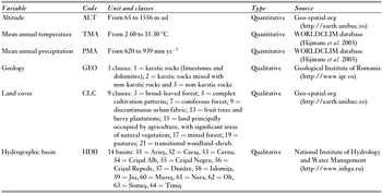
This study is focused on groundwater habitats, void networks and pools, in caves of the Romanian Carpathians. Point-sampled data for biological (Appendix 1, Table S1, see supplementary material at Journals.cambridge.org/ENC) and habitat variables (Table 1) were gathered from several sources. Three quantitative and three qualitative environmental variables that describe the surface-cave ecosystem were included in the model.
Environmental variables used in modelling.

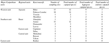
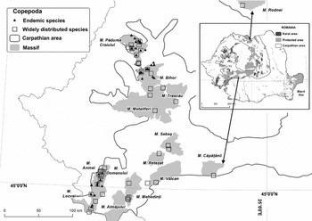
Copepod distribution data were compiled from different sources, including: (1) 38 published sources; (2) existing databases of the ‘Emil Racoviţă’ Institute of Speleology, and (3) personal surveys (the list of all references is available on request). Two ecological categories of copepods were considered, hypogean and epigean, based on the copepods restricted to groundwater and surface habitats, respectively. Species presence data were georeferenced as point-sampled data using Google Earth Pro and ArcGIS Desktop (ESRI [Environmental Systems Research Institute] 2010). The final list includes 238 records (Appendix 1, Table S1, see supplementary material at Journals.cambridge.org/ENC). The minimum number of records for a species was one and the maximum was 18. The habitat suitability model was applied at the species and genus levels for the seven taxa having more than 10 entries in the database (Fig. 1, Table 2).
Number of sampling sites, number of copepod species, and number of hypogean and endemic copepod species for each sampled Carpathian unit included in habitat suitability modelling.

Distribution of modelled copepods across the Romanian Carpathians. Protected areas layer available from URL http://www.mmediu.ro/protectia_naturii/protectia_naturii.htm. (last access date on December 1, 2011)

For accuracy, all data were projected in the Stereo70 coordinate system using the Dealul_Piscului_1970 datum between the spatial scales of 1:100 000 and 1:200 000.
Linear regression analysis
To obtain the pattern of ecological conditions for each species location, linear regression analysis (ordinary least squares [OLS] and geographically-weighted regression [GWR]) was performed using spatial statistics in ArcGIS 9.3.1 (ESRI 2010). In the first step, OLS was used to model and examine the statistically significant factors behind observed spatial distribution patterns. Once the significant factors were selected, the GWR was computed over a spatial scale based on neighbours’ measures in order to remove the assumption of spatial stationarity in the distribution modelling. The statistically significant variables identified by the linear regression analysis were kept for the habitat suitability modelling (Fig. 2).
Simplified diagram showing the statistical analyses performed to model taxa habitat suitability. OLS = ordinary least squares; VIF = variance inflation factor; GWR = geographically-weighted regression.

The significant factors were selected by computing OLS. Akaike's information criterion (AIC) (Akaike Reference Akaike1974) was used to select the most parsimonious model. The Jarque-Bera test was used to evaluate the goodness of fit of the models, indicating if the residual values (the over- and under-predictions) had a normal distribution. If they did not, the model was biased. Multicollinearity was detected by calculating the variance inflation factor (VIF), an index measuring how much the variance of the estimated regression coefficient increased because of collinearity. The VIF ranges from 1.0 to infinity, and we considered its threshold value should be less than 7.5 to avoid multicollinearity (Kenneth et al. Reference Kenneth, Strager and Welsh2013). Environmental variables with a VIF greater than 7.5 were removed one by one until the VIF indicated the model was not biased. An adjusted R2 value was used to measure the proportion of the variation in the dependent variable (species) accounted for by the environmental variables.
OLS allowed simultaneous processing of quantitative and qualitative variables. For all qualitative variables integer codes were associated with their values, having a minimum of three integer codes per variable (Table 1). The analysis took into account the unique identification of each database record, which further was associated with all the predictors’ values. In this regard, VIF was very useful in discarding variables that contained redundant information.
The GWR created a coefficient surface for each environmental variable showing where the relationships were strongest. As for OLS, an AIC value and adjusted R2 were computed to test for good model performance. The goodness of fit was tested using the spatial autocorrelation (Morans I) tool, in order to check for the spatial autocorrelation of model residuals. When a good model was found, the residuals reflected random noise (Goodchild Reference Goodchild1986). The correlation coefficients were estimated using nearby feature values. Adaptive kernel estimation was used in the present models, with the number of neighbours ranging from 5 to 15, in order to determine the best model (Fotheringham et al. Reference Fotheringham, Brunsdon and Charlton2002).
Habitat suitability model
The statistically significant variables were used to develop habitat suitability models and predict species-environment relationships and spatial patterns across spatial scales. Năpăruş and Kuntner (Reference Năpăruş and Kuntner2012) developed a habitat suitability model using the ModelBuilder environment from ArcGIS Desktop 9.3.1 (ESRI 2010). We applied the same model for seven different copepod taxa to visualize their directional distribution trend and the areas with high, moderate and low habitat suitability.
The directional distribution trend was computed for each taxon as an elliptical area centred on the mean of all localities inhabited by that taxon. We used the option with three standard deviations to maximize the potential species distribution to cover c. 99% of all feature centroids (Mitchell Reference Mitchell2005). The model shows the central tendency and its spatial orientation for each species’ distribution as an indication of potential trend dispersion. The directional distribution represents a species’ potential target area for habitation (Năpăruş & Kuntner Reference Năpăruş and Kuntner2012). In the case of copepods, we assumed that each taxon's potential habitat exhibited preferences for a corridor with a total span of five degrees of longitude. In this potential distribution area, we extracted the values for the environmental predictors corresponding to each taxon's database records in order to obtain their frequency and then to classify them as high, moderate or low frequency. In the cases of two widely distributed taxa, when only two classes were depicted we preferred to classify the values as high and moderate. These frequency values were used to identify, within the species directional distribution, similar values, which were reclassified to represent habitat suitability (reclassified as high = 3, moderate = 2 and low = 1). In order to obtain a scale of suitability from 1 (low) to 3 (high), we used the weighted sum tool, by multiplying the designated field values for each environmental parameter with the specified weight. The weights for the habitat suitability were assigned by dividing 1.0 (100%) among the resulted correlated parameters. ‘NoData’ values were ignored. If the species was correlated with two environmental parameters, we combined them by assigning equal weights (0.5). In the case of a single environmental parameter, the given weight value was unity.
The model was finalized by fitting the habitat suitability dot representation to a local scale with a radius of nine cell units (720 m) by using focal statistics analysis (Guisan & Thuiller Reference Guisan and Thuiller2005). All cells whose centre fell inside this radius were included in processing the neighbourhood.
Among the seven habitat suitability maps, two are given here as examples (the hypogean species Acanthocyclops sp. and the epigean species Bryocamptus zschokkei) (other maps are provided in Appendix 1, Figs S1–S5, see supplementary material at Journals.cambridge.org/ENC).
RESULTS
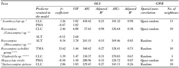
Except for Spelaeocamptus spelaeus (adjusted R2 = 0.26), the GWR results explained more than 50% of the taxon-environment relationship (Table 3). Of the six predictors included in the model, the main drivers were temperature and precipitation for epigean species, while land cover was significant mainly for hypogean taxa.
Summary of OLS and GWR statistical models for seven copepod taxa in groundwater habitats of the Carpathians (all data are statistically significant at p < 0.05). OLS = ordinary least squares; VIF = variance inflation factor; GWR = geographically-weighted regression; PMA = mean annual precipitation; TMA = mean annual temperature; ALT = altitude; CLC = land cover. 1Hypogean taxa. For harpacticoids, we used Wells (Reference Wells2007) and, for cyclopoids, Dussart and Defaye (Reference Dussart and Defaye2006). Each selected group is considered as an ecological unit, which is not necessary a taxonomically defined taxon. *Acanthocyclops sp. includes the following species currently unified in the kieferi group of this genus: A. balcanicus bisaetosus, A. deminutus, A. kieferi, A. milotai, A. plesai, A. propinquus, A. reductus, and A. transylvanicus. **Bryocamptus (Limocamptus) sp. includes the closely-related B. (L.) echinatus, 1B. (L.) dacicus and Pilocamptus georgevitchi, which differ morphologically from the ‘zschokkei’ group by their three-segmented leg 1 structure. ***Bryocamptus (Rheocamptus) sp. includes species with reduced leg segmentation and armature: B. (R.) typhlops and B. (R.) unisaetosus. ****Bryocamptus zschokkei group includes species characterized by untransformed segmentation and armature: B. (B.) pygmaeus, B. (B.) spinulosus, B. (B.) zschokkiei caucasicus, B. (B.) zschokkei tatrensis, and B. (B.) zschokkei zschokkei. *****Elaphoidella sp. includes: E. phreatica, E. phreatica pseudophreatica, E. putealis, E. romanica and E. winkleri.

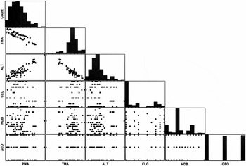
Scatter plot matrices to explore bivariate cause-effect relationships between environmental parameters through β-coefficients recovered only a positive correlation between altitude and mean annual precipitation (PMA), and negative correlations between altitude and mean annual temperature (TMA) and between TMA and PMA (Fig. 3).
Scatter plot matrices displaying relationships among the environmental parameters for all 238 records in the database. PMA = mean annual precipitation; TMA = mean annual temperature; ALT = altitude; CLC = land cover; HDB = hydrographic basin; GEO = geology.

The residuals reflected random noise for Bryocamptus (Rheocamptus) sp., Bryocamptus zschokkei group, Elaphoidella sp. and Spelaeocamptus spelaeus, and quasi-random noise for Acanthocyclops sp., Bryocamptus (Limocamptus) sp. and Megacyclops viridis, as indicated by the spatial autocorrelation analysis
Acanthocyclops sp., Bryocamptus (Limocamptus) sp., Elaphoidella sp. and S. spelaeus had positive correlations with land cover (CLC) (Table 3), showing a preference for areas covered by broad-leaved and mixed forests (Appendix 1, Table S2, see supplementary material at Journals.cambridge.org/ENC). S. spelaeus was also correlated with areas covered by agricultural fields. Areas with discontinuous urban fabric, pastures, fruit tree plantations and transitional woodland-shrub were associated with low and moderate probabilities of harbouring copepod species. Megacyclops viridis and Acanthocyclops sp. had negative correlations with PMA (Table 3). M. viridis showed preferences for areas with precipitation of 630–865 mm yr−1, with high probabilities of being encountered in areas with precipitation of 710 mm yr−1. For Acanthocyclops sp. the most suitable areas were those with precipitation of 650–800 mm yr−1. This species had a low probability of occurrence in areas with high precipitation rates (810–860 mm yr−1). The epigean Bryocamptus zschokkei group was strongly correlated with temperature, with the probability of occurrence increasing from 8.2 to 9.1°C (Fig. 4). The altitude was important for the other two Bryocamptus groups (Limocamptus and Rheocamptus), the first having high chances of being encountered in areas with elevations of 274–540 m above sea level (asl), while the second had a wider elevation range of 344–1269 m asl.
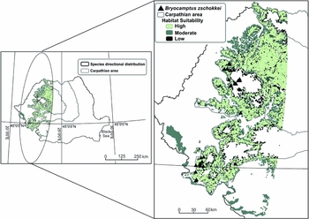
Habitat suitability map for the epigean Bryocamptus zschokkei. Triangles = current specimen records. Predicted suitable habitats are represented by light grey (high probability of taxa occurrence), dark grey (moderate probability of taxa occurrence) and black dots (low probability of taxa occurrence).

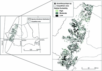
All the considered taxa were sampled from the Romanian Carpathian caves, but the areas predicted to be suitable were not consistent with the observed distributions in the limestone areas; all taxa had high probabilities of occurrence outside these areas. For the B. (Limocamptus) species, a high probability of suitable habitats was detected along a north-south distribution outside the Romanian Carpathians, in areas with lower elevation (namely south of Banat and more scattered suitable habitat in the north-west of Romania) (Appendix 1, Fig. S1, see supplementary material at Journals.cambridge.org/ENC). The B. (Rheocamptus) species have the largest areas of suitable habitat distributed north-east to south-west (Appendix 1, Fig. S2, see supplementary material at Journals.cambridge.org/ENC). The model predicted large areas of suitable habitat with high probabilities of B. zschokkei group occurrence, with a north-south distribution (Fig. 4). M. viridis, currently widespread in Romania, showed mainly moderate probabilities of occurrence in western Romania, distributed along a north-west to south-east axis (Appendix 1, Fig. S3, see supplementary material at Journals.cambridge.org/ENC). Compared to epigean species, the suitable areas predicted by the habitat suitability model overlapped more closely the observed distribution of hypogean taxa Acanthocyclops sp. (Fig. 5), Elaphoidella sp. (Appendix 1, Fig. S4, see supplementary material at Journals.cambridge.org/ENC) and S. spelaeus (Appendix 1, Fig. S5, see supplementary material at Journals.cambridge.org/ENC), whose more restricted predicted distribution was oriented towards limestone areas, the first two species being distributed along a north-west to south-east axis and the last along a north-east to south-west axis.
Habitat suitability map for the hypogean Acanthocyclops sp. Triangles = current specimen records. Predicted suitable habitats are represented by light grey (high probability of taxa occurrence), dark grey (moderate probability of taxa occurrence) and black dots (low probability of taxa occurrence).

DISCUSSION
Cave assemblages enclosing epigean and hypogean species were useful in predicting the surface environment health related to land-use and climate variables. The habitat suitability model was easily applied because of its simple customizing process, high degree of visualization, and adaptivity for each taxon's requirements. Based on spatial autocorrelation analysis, the performance of the final models was adequate, reflecting the random and quasi-random noise characteristic of good models. According to Osborne et al. (Reference Osborne, Foody and Suárez-Seoane2007) and Bacaro et al. (Reference Bacaro, Santi, Rocchini, Pezzo, Puglisi and Chiarucci2011), spatial autocorrelation in species distribution modelling, as a common property of ecosystems, is an important feature usually missed or inadequately considered.
Overall our model achieved a good fit, with GWR adjusted R2 values approaching 1. The low adjusted R2 in S. spelaeus case is not unexpected, knowing that species distribution modelling attempted for hypogean populations from the Jura Mountains explained 36% of the average deviance of hypogean species distribution (Castellarini et al. Reference Castellarini, Malard, Dole-Olivier and Gibert2007). Our results suggest a proper selection of predictor variables in most of the cases. In the present study, depending on taxon requirements, four out of six predictors were retained in the habitat suitability models: altitude, mean annual precipitation, mean annual temperature and land cover.
The north-west to south-east distribution, with low probability of occurrence outside the known distribution range of Acanthocyclops sp., is probably due to the narrow niche requirements of this highly diversified and endemic genus (Galassi et al. Reference Galassi, Huys and Reid2009). All the species belong to the kieferi species complex, a diversified group within the groundwater of Romania (Iepure & Defaye Reference Iepure and Defaye2008). The distribution of A. transylvanicus was not found to be dependent on the local precipitation (Meleg et al. Reference Meleg, Fiers, Robu and Moldovan2012), suggesting the importance of scale when assessing biodiversity, as emphasized by Stoch and Galassi (Reference Stoch and Galassi2010).
Our model showed a narrow range of suitable areas for Elaphoidella sp. and S. spelaeus, both with probabilities of occurrence along the western extremities of the Romanian Carpathians. The predicted probabilities of occurrence outside limestone areas for both species, not overlapping their current range in caves, show their possible distribution in other groundwater habitats, such as interstitial waters of surface rivers or springs (Damian-Georgescu Reference Damian-Georgescu1970). For S. spelaeus, the areas predicted to be most suitable were consistent with the observed site-specific distribution in caves of the western Carpathians (Fiers & Moldovan Reference Fiers and Moldovan2008).
For the hypogeans Acanthocyclops sp., Elaphoidella sp. and S. spelaeus, the predicted suitable habitats were more or less restricted to the observed distribution patterns. Their distribution may reveal limited ability to disperse and exploit hydrological connectivity through migration, as in the Jura Mountains (Castellarini et al. Reference Castellarini, Malard, Dole-Olivier and Gibert2007). There the occurrence of E. phreatica is related to high elevation, unlike in the present study where elevation was not a significant predictor for Elaphoidella species, including E. phreatica. Only the epigeans Bryocamptus (Limocamptus) sp. and Bryocamptus (Rheocamptus) sp. had distributions correlated with elevation. For the B. (Limocamptus) group, a high probability of suitable habitats occurred outside the limestone areas of the Romanian Carpathians at lower elevations, suggesting either this sub-genus’ preference for non-limestone habitats (Damian-Georgescu Reference Damian-Georgescu1970), or its occurrence is the result of being washed from the surface into the cave. The B. (Rheocamptus) group showed the largest spectrum of suitable habitats, both representatives occurring in a wide range of habitats (mosses, springs, wells, peat bogs and groundwater). Although B. zschokkei has occurred throughout the temperature range, it was the only group where occurrence was correlated with temperature. The habitat suitability model predicted only rather low probabilities of suitable habitats for M. viridis, model performance was probably influenced by the cosmopolitan distribution of this species encompassing a large number of ecological features across their distribution range (Osborne et al. Reference Osborne, Foody and Suárez-Seoane2007).
Climate variables were directly related with the epigean taxa, and were the most important drivers explaining their distribution in caves. The modelled suitable habitats underline their transitory status within the caves, as has been determined at smaller spatial scales (Meleg et al. Reference Meleg, Fiers, Robu and Moldovan2012; Moldovan et al. Reference Moldovan, Meleg and Perşoiu2012). Their observed sensitivity to changes in temperature or precipitation indicate epigean taxa might find protection from climatic disturbance inside caves. Their persistence within cave assemblages might impact the resident hypogean assemblages, with biotic interactions leading to ecological and populations’ instability; narrowly-distributed hypogean taxa more susceptible to ecological disequilibrium and habitat loss (Cardoso et al. Reference Cardoso, Borges, Triantis, Ferrández and Martín2010) will either adapt or become endangered.
Our work emphasizes for the first time the importance of land use and anthropogenic impact (Vandewalle et al. Reference Vandewalle, de Bello, Berg, Bolger, Dolédec, Duds, Feld, Harrington, Harrison, Lavorel, Silva, Moretti, Niemelä, Santos, Sattler, Sousa, Sykes, Vanbergen and Woodcock2010) on habitat suitability for groundwater copepods. For the hypogean Acanthocyclops sp., Bryocamptus (Limocamptus) sp., Elaphoidella sp. and S. spelaeus, we found low and moderate probabilities of occurrence in areas where the above-cave habitats were covered by sparsely vegetated areas, fruit tree plantations within a discontinuous urban matrix, or pastures. The forests and land used in traditional agriculture appear important for underground copepod population persistence.
Deforestation is directly linked to climate changes that lead to temperature increases, shifts in precipitation patterns and drying out of the vegetation (Davin & de Noblet-Ducoudré Reference Davin and de Noblet-Ducoudré2010). The environmental parameters mirrored the responses of groundwater communities to surface-groundwater dynamics when more than one parameter was in the final model. For example, Acanthocyclops sp. display preferences for forested areas and moderate amounts of precipitation.
Both the forest and soil play an important role in cave evolution and ecosystem dynamics, as sources of organic matter that concentrate within the void network and in pools populated by copepods (Williams Reference Williams, Jones, Culver and Herman2004; Meleg et al. Reference Meleg, Fiers, Robu and Moldovan2012). Water balance is also important in determining and sustaining the terrestrial vegetation, and thus the land cover (Neilson Reference Neilson1995). The water input has a major role in limestone dissolution, and in cave and fissure formation as suitable habitats for copepod populations. Water also governs the dispersal of organisms and plays an important role in the transportation of organic matter and epigean organisms below ground (Moldovan et al. Reference Moldovan, Meleg and Perşoiu2012).
Intensive cultivation also raises concern for use of nitrogen-rich fertilizers and pesticides, such substances being harmful below ground when quickly washed into caves, as happens when the filtration process is ineffective due to soil erosion. Organic pollution leads to depletion of subterranean communities (Hancock et al. Reference Hancock, Boulton and Humphreys2005) and groundwater copepod communities are no exception. GIS modelling revealed that hypogeans are more endangered cave assemblages than those of epigeans, because they have narrow distribution ranges and the local effect of surface pollution would be more intense. Pollution at the aquifer scale impacts the inhabited voids by generating heterogeneous patches with different degrees of alteration, ecological disequilibrium and subterranean fauna depletion or extinction (Mösslacher & Notenboom Reference Mösslacher, Notenboom and Gerhardt1999).
The low predicted occurrence of studied taxa in areas facing anthropogenic pressure through land-use changes associated with climate variations emphasizes the potential use of copepods as bioindicators for the dynamic surface-groundwater system. Groundwater invertebrates also maintain a high water quality through water purification, bioremediation, and water infiltration and transport (Boulton et al. Reference Boulton, Fenwick, Hancock and Harvey2008; Griebler et al. Reference Griebler, Stein, Kellermann, Berkhoff, Brielmann, Schmidt, Selesi, Steube, Fuchs and Hahn2010). Their persistence below ground is an indirect measure of surface-groundwater system health.
Given its computational efficiency and reliability, GIS is a useful tool for identifying endemism and biodiversity hotspots at local and regional scales. GWR and the designed habitat suitability model provided a framework for coupling distribution patterns to ecosystem dynamics for both epigean and hypogean species. Both human induced stressors across space and climate change across time may act as ecological barriers for cave assemblages that may lead to disturbed subterranean habitats.
CONCLUSION
This study provides evidence for the importance of managing the landscape in limestone areas to conserve the groundwater resources and copepod biodiversity. We propose a model for groundwater protection based on the sustainable use of the surface land. Surface land management should be oriented towards promoting traditional agricultural practices and soft deforestation, and reforestation when needed. Most of the known distribution of the analysed communities are within protected areas (national and natural parks and Natura 2000 sites) where sustainable practices are promoted according to EU Habitats Directive (92/43/EEC; European Commission 2013) and Groundwater Directive (2006/118/EC; European Council 2006), as well as Romanian Law no. 49/2011 regulating natural protected areas, conservation of natural habitats, wild flora and fauna in Romania and the Romanian Forest Code. We have identified areas not included in the current protected areas that should also be managed in order to preserve the groundwater and its fauna. Our assessment is relevant in understanding the potential impact of the key driving forces of cave assemblages’ distribution as a proxy to the interconnected environmental surface-subterranean systems in limestone areas.
ACKNOWLEDGEMENTS
Ioana Meleg and Magdalena Năpăruş contributed equally to this work. We thank Gregor Aljančič, Andreea Guţu, Matjaž Kuntner and Ionuţ Şandric for help and discussions and ESRI Romania for software support. We thank the anonymous reviewers, and journal editors that considerably improved the content quality and clarity. Craig Moore was very helpful in improving the English of the manuscript. The study was financially supported by the Romanian Academy; part of the data collection was supported through the KARSTHIVES Project PCCE_ID_31/2010 funded by CNCS-UEFISCDI.