

1. Introduction
The response of a wall-bounded flow to a sudden change in surface roughness is of considerable interest for several reasons. Such flows are common in nature, as when an offshore wind meets a coastline, or when the wind blows over a changing terrain such as a change from forest to grassland. They are found in biological flows where fish can exhibit different surface textures along their length, and in industrial applications where the roughness height can abruptly vary at the junction between two plates or pipes. Second, the response to a change in surface roughness is both length and time scale dependent. Consequently, it provides a severe test of turbulence models.
Previous work on such step changes indicates that the adjustment of the flow to its new wall condition is often rather slow (Smits & Wood Reference Smits and Wood1985). For example, in a study of a boundary layer experiencing a change from smooth to rough conditions, Antonia & Luxton (Reference Antonia and Luxton1971) found that self-preservation (that is, the flow scales with local variables sometimes referred to as being self-similar) was re-established after approximately  $20\delta _0$, where
 $\delta _0$ was the boundary layer thickness at the point where the surface condition changed. For a step change from rough to smooth conditions (Antonia & Luxton Reference Antonia and Luxton1972), the relaxation was far from complete after
 $16\delta _0$, corresponding to the end of the measurement domain. In both cases, the relaxation could be described in terms of the growth of an inner layer. The height of this layer,
 $\delta _i$, marks the outward extent of the flow that is influenced by the new boundary condition, and the rate at which it grows appears to be typical of a thin shear layer. For example, Wood (Reference Wood1982) found that for step changes in surface roughness it increased approximately as
 $x_s^{0.8}$, where
 $x_s$ was the distance downstream of the step. Similar conclusions were reached by Cheng & Castro (Reference Cheng and Castro2002) and Efros & Krogstad (Reference Efros and Krogstad2011) regarding the smooth-to-rough response, and by Mulhearn (Reference Mulhearn1978); Chamorro & Porté-Agel (Reference Chamorro and Porté-Agel2009); Loureiro et al. (Reference Loureiro, Sousa, Zotin and Freire2010); Hanson & Ganapathisubramani (Reference Hanson and Ganapathisubramani2016) and Li et al. (Reference Li, de Silva, Rouhi, Baidya, Chung, Marusic and Hutchins2019) for the rough-to-smooth response. The study by Hanson & Ganapathisubramani (Reference Hanson and Ganapathisubramani2016), being the most recent of the rough-to-smooth transition studies, is particularly notable for its extensive measurements, although the domain of interest was limited to
 $x_s/\delta _0 <16.4$.
It should be noted that these conclusions and observations apply only to boundary layers (Hanson & Ganapathisubramani (Reference Hanson and Ganapathisubramani2016) and Li et al. (Reference Li, de Silva, Rouhi, Baidya, Chung, Marusic and Hutchins2019) provide a more complete literature review), and these investigations have been restricted to distances of no more than  $x_s/\delta _0 =20$. Here, we explore instead how a fully developed turbulent pipe flow responds to a change in wall condition from rough to smooth, and we examine the response up to a distance of
 $x=x_s/R = 120$, where
 $R$ is the radius of the pipe. The response of a confined flow such as that in a pipe is fundamentally different from that of a boundary layer, even at a comparable Reynolds number. In essence, the flow near the wall that had been retarded by the roughness begins to accelerate immediately when the surface changes to being smooth. By continuity, therefore, the flow across the entire width of the pipe responds to the change in roughness, and the concept of an internal layer no longer strictly applies.
We find that the flow is not fully equilibrated even at the farthest downstream station and that the relaxation displays a second-order response where the Reynolds stresses first fall below their self-similar levels before slowly approaching them. To help interpret the flow response, we connect our observations to the equations of motion and develop physical models of the response by using a scale decomposition.
2. Experimental methods
Experiments were conducted in a straight pipe, radius  $R=19.1\ \textrm {mm}$, filled with water driven at a bulk velocity of
 $U_b=3.45\ \textrm {m} \ \textrm {s}^{-1}$ resulting in a diameter-based Reynolds number of
 $Re_D = U_b D/\nu =1.31\times 10^5$, where D is the pipe diameter and ν is the kinematic viscosity. The flow is initially developed in a smooth section of length
 $240R$, passes through a
 $192R$ long roughened section with equivalent sand grain roughness
 $k_S=415\ \mathrm {\mu }\textrm {m}$ or
 $k^+ = k_s u_\tau /\nu = 66$, where
 $u_\tau$ is the friction velocity, then back to a smooth pipe, which marks the start of the test section. Velocity measurements were taken at
 $x=4.4$ 6.4, 9.2, 13.4, 19.4, 28.4, 41.2, 60, 80, 100 and 120, where the step change occurs at
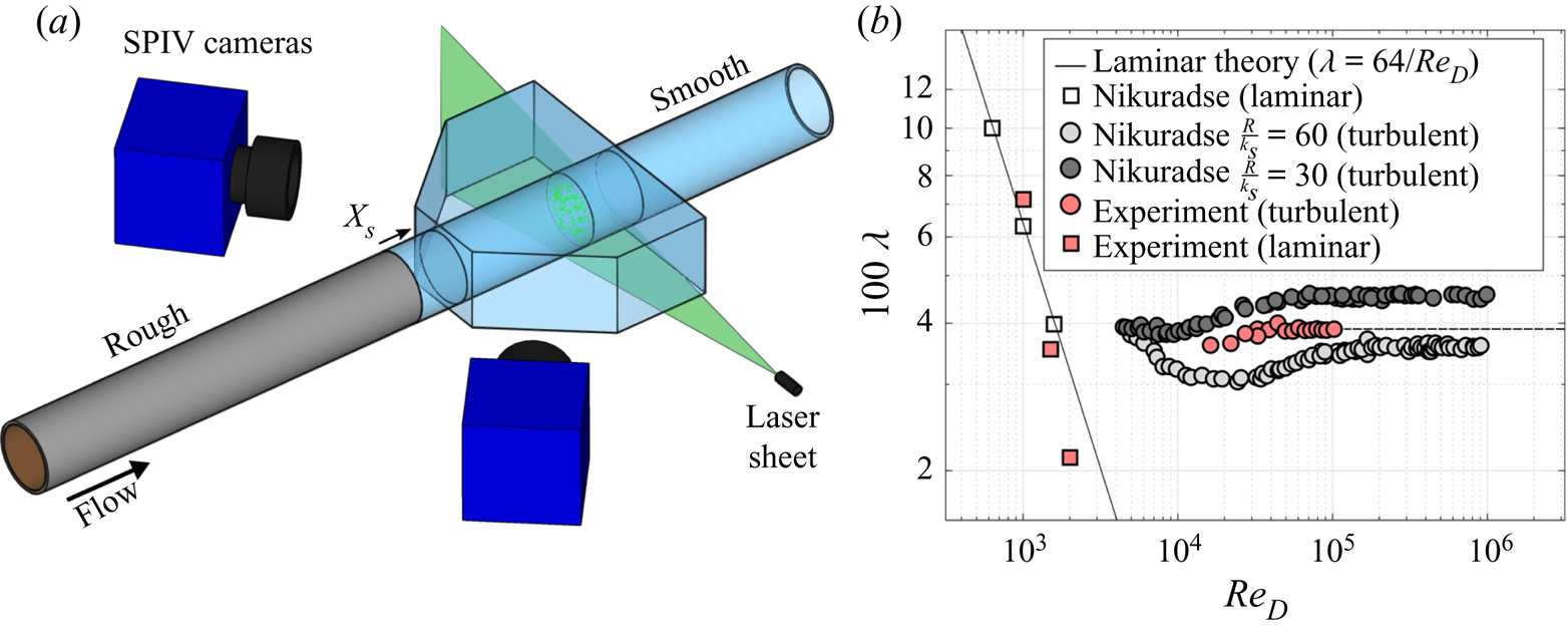
 $x=0$. The experimental configuration is shown schematically in figure 1(a).
 $(a)$ SPIV experimental schematic and
 $(b)$ estimation of our equivalent sand grain roughness by comparing the measured coefficient of resistance
 $\lambda$ as it varies with Reynolds number to the original results from Nikuradse (Reference Nikuradse1950).
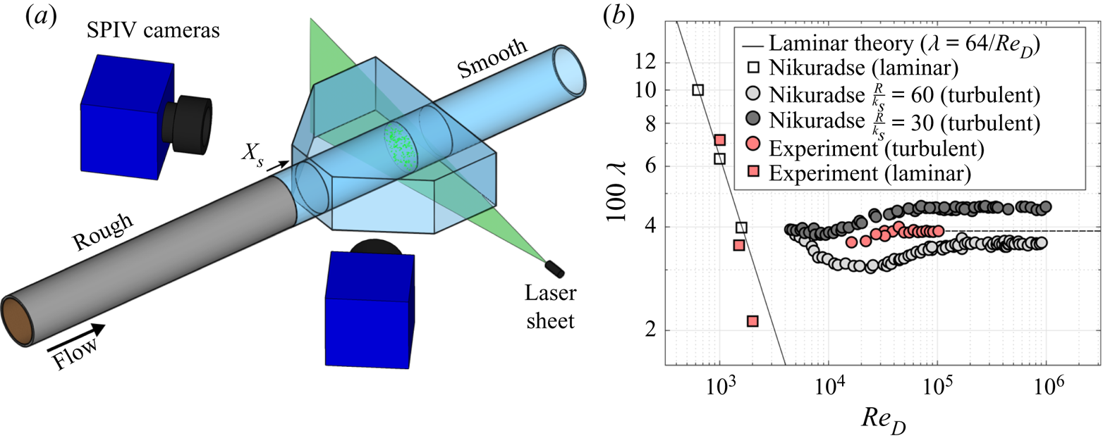
The rough pipe was made using a process originally employed by Nikuradse (Reference Nikuradse1950) where sand grains of consistent size (54 grit garnet sandblasting media) were fastened to an aluminium pipe with epoxy. To achieve a homogeneous layer of roughness, the epoxy was first evenly applied to the inside of the aluminium pipe, and then the pipe was mounted vertically, filled with the sand grains, and left to dry. Once dry, the loose sand grains were discarded, leaving an even sand grain layer behind. The equivalent sand grain roughness was estimated by comparing the measured coefficient of resistance  $\lambda$ – calculated from the pressure drop measurements in the rough pipe sections – to the data of Nikuradse (Reference Nikuradse1950), as plotted in the style of Schlichting (Reference Schlichting1968) in figure 1(b).
Velocity measurements were taken using stereoscopic particle image velocimetry (SPIV), as shown in figure 1(a). Two 5.5 mega-pixel sCMOS cameras recorded images of a plane illuminated with a dual-pulsed 50 mJ Nd:YAG laser. The flow was seeded with  $10\ \mathrm {\mu }\textrm {m}$ hollow glass spheres (density
 $1.1\ \textrm {g} \ \textrm {cm}^{-3}$). A water-filled acrylic test section, designed such that the cameras and laser were normal to their respective acrylic walls, surrounded the glass pipe to minimize image distortion. A total of 11 000 image pairs, acquired at a frequency of 25 Hz, were recorded at each downstream location. Images were processed in DaVis 8.3 using a multi-pass cross-correlation method with interrogation window sizes decreasing to a final size of
 $32 \times 32$ pixels with 50 % overlap, resulting in a vector grid spacing of 0.26 mm. In processing the velocity field, the universal outlier detection algorithm (Westerweel & Scarano Reference Westerweel and Scarano2005) indicated that at least 95 % of the velocity vectors resulted from the first choice of correlation peaks, while most others were the second choice with only a few outliers that needed to be removed and interpolated.
Pressure measurements were made in both the rough and smooth pipes using a custom freestanding manometer, accurate to  ${\pm }7.7\ \textrm {Pa}$, which corresponds to a 2.9 % uncertainty in the pressure gradient, at the worst. To determine the pressure drop in the rough section (
 $192R$ long), measurements were made 64
 $R$ and 128
 $R$ from the start of the roughened section. To measure the pressure development downstream of the step, a custom pipe section was fitted temporarily, consisting of a smooth aluminium pipe fitted with 20 pressure taps with gradually increased spacing from
 $x=6, 6.7, 7.3, \ldots , 9.3$,
 $10.7, \ldots , 17.3$,
 $21.3, \ldots , 49.3\ \textrm {radii}$ downstream. The friction velocity of the rough-wall fully developed flow was measured to be
 $u_{\tau _r}=0.45 \ \textrm {m} \ \textrm {s}^{-1}$, and for the smooth-wall fully developed pipe flow it was
 $u_{\tau _0}=0.16\ \textrm {m} \ \textrm {s}^{-1}$.
3. Results
In a fully developed pipe flow, the area- and time-averaged pressure gradient  $\langle {\text {d}P}/{\text {d}x} \rangle$, where P is the pressure field, balances the\query[-2pc]{Q7} wall shear
 $\tau _w$ exactly, but when the flow is in a state of development the streamwise gradient of the momentum flux
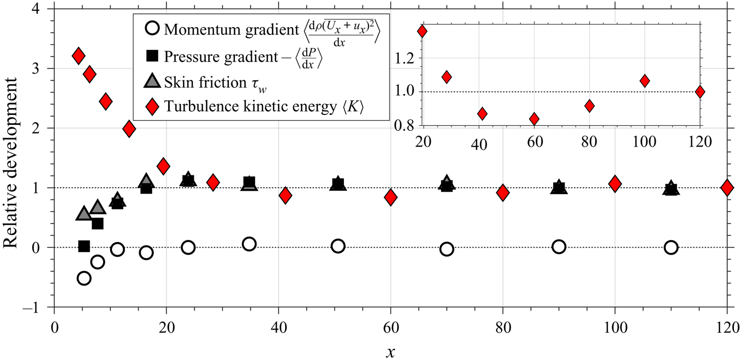
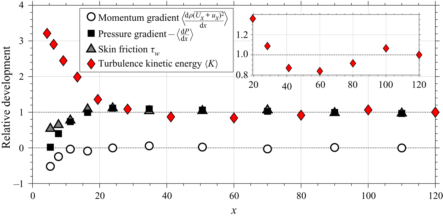
 $\langle {\text {d}\overline {(U_x+u_x)^2}}/{\text {d}x} \rangle$ also contributes to the force balance. Figure 2 shows the various contributions made by the momentum gradient, pressure gradient and wall shear in our experiment as the flow responds to the step change. The development of the area-averaged turbulence kinetic energy
 $\langle K \rangle$ is also shown. This figure displays relative development, where the pressure gradient, skin friction and turbulence kinetic energy are normalized by their values at the farthest downstream location, which is taken as an estimate of the fully relaxed state. Because the momentum gradient approaches zero far downstream, it is normalized by the smooth friction velocity and pipe radius. From this point onward, all quantities are given non-dimensionally, normalized using
 $R$ and
 $\tau _0 = \rho {u^2_\tau }_0$, where
 $\tau _0$ is the wall shear stress value expected to occur very far downstream of the step change. (A more detailed discussion of the pressure distribution can be found in Van Buren, Hellström & Smits (Reference Van Buren, Hellström and Smits2019).) We see that for a short region downstream of the step change the wall shear, momentum gradient and pressure gradient are all lower than in the fully developed smooth-wall case. These quantities recover relatively quickly, however, and by
 $x=20$ they have approximately reached their fully developed values. Close inspection of the turbulence kinetic energy level, however, reveals small oscillations that persist much further downstream. This oscillatory response of the flow statistics, shown here by the turbulence kinetic energy, will be referred to throughout the text as a second-order response (more strictly it is a higher-order response).
Streamwise relative development of the pressure gradient, skin friction, streamwise momentum gradient and the cross-sectional area average of the turbulence kinetic energy. Here,  $x=x_s/R$.
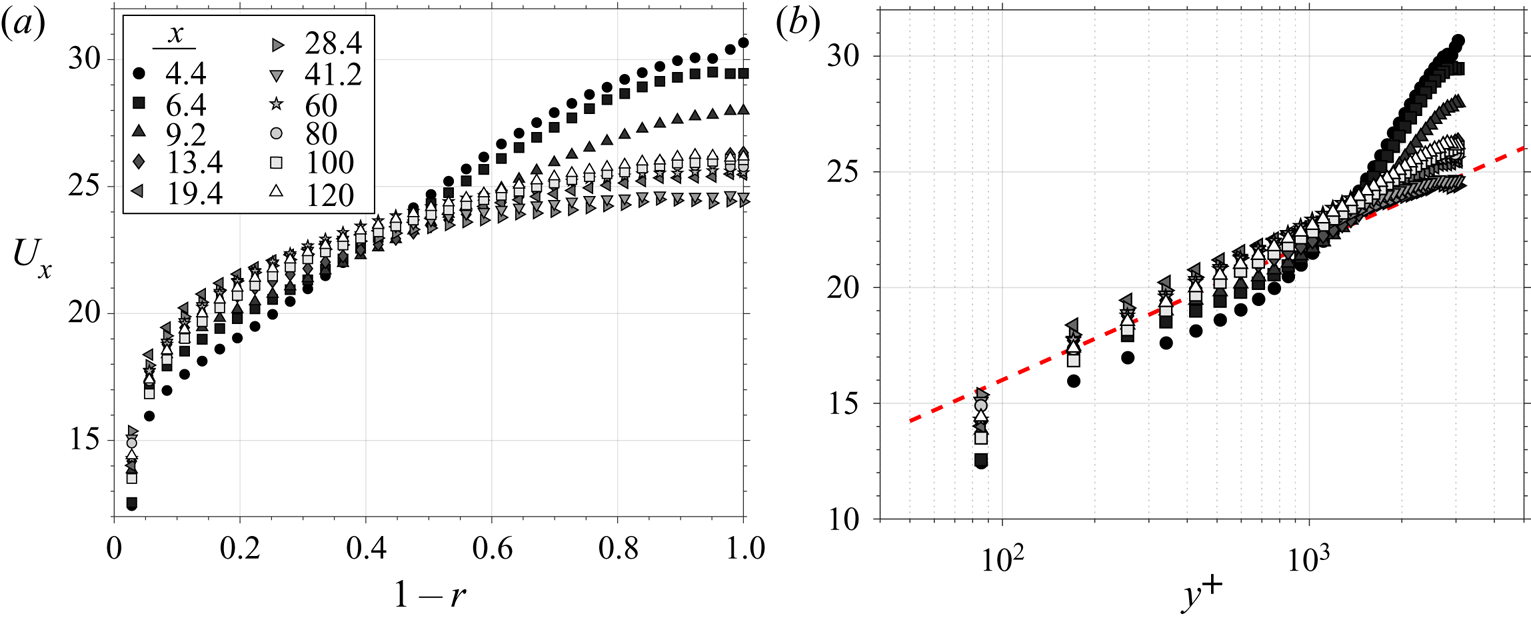
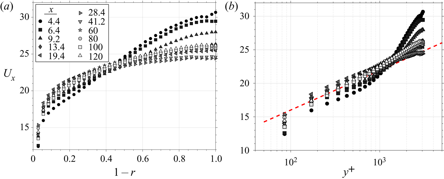
The mean flow response is shown in linear and semi-log coordinates in figure 3. Here,  $r$ is the non-dimensional radial coordinate (distance from the pipe centre divided by
 $R$). Downstream of the step, the mean streamwise velocity
 $U_x$ increases near the wall (due to the drop in wall stress) and decreases at the centre instantly (due to continuity and the geometrical constraints of an enclosed flow), almost pivoting about a central point like a seesaw. This characteristic feature distinguishes enclosed flows, like those in pipes and channels, from boundary layer flows; perturbed boundary layer flows have the opportunity to grow, whereas enclosed flows must absorb the change in other ways.
Mean streamwise velocity profile development in  $(a)$ linear and
 $(b)$ semi-log plotting style. The red line indicates the log-law slope for the fully developed smooth case. Note that the mean velocity is normalized by the friction velocity
 $u_{\tau _0}$ for the smooth wall at the same bulk flow Reynolds number (as are all other velocities, unless otherwise stated) and
 $y^+ = y u_{\tau _0} / \nu$.
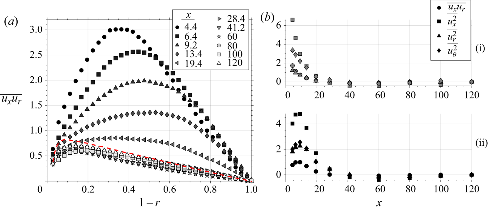
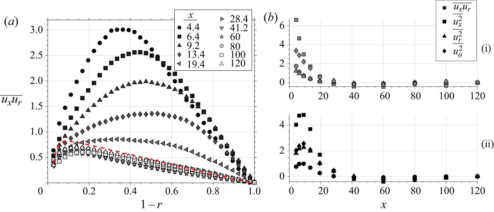
The downstream development of the Reynolds shear stress profiles is shown in figure 4. Here,  $y$ is the non-dimensional distance from the wall (distance from the wall divided by
 $R$). Downstream of the step, the turbulence generally decays rapidly and overshoots the fully developed values. For a considerable distance – from
 $x=20$ to at least
 $x=120$ downstream – the turbulence is lower than the fully developed smooth-wall case. Adding to the complexity, the flow towards the wall responds differently than the flow near the centre, where in the centre the turbulence increases initially before decaying downstream. Although all Reynolds stresses display a similar response, they decay at different rates downstream – seen in figure 4(b).
Streamwise development of the  $(a)$ Reynolds shear stress
 $\overline {u_x u_r}$ profile and
 $(b)$ the change in Reynolds stresses
 $\overline {u_x^2}$,
 $\overline {u_r^2}$
 $\overline {u_\theta ^2}$ and
 $\overline {u_x u_r}$ at (i)
 $y=0.2$ and (ii)
 $y=0.8$. The red line is the profile for a smooth-wall, fully developed pipe flow at this Reynolds number.
To address how the mean flow response in the pipe impacts the turbulence response, and why the turbulence shows this very slow, second-order response, we will now examine the equations of motion in detail.
3.1. Equations of motion
Consider an incompressible pipe flow in cylindrical coordinates ( $x,r,\theta$) subject to a step change in surface roughness (rough to smooth) at
 $x=0$. The flow velocity and pressure are separated into their mean (
 $U_i$,
 $P$) and fluctuating components (
 $u_i$,
 $p$). We assume that ensemble averages are steady in time (that is,
 $\partial \overline {(\cdot )} / \partial t = 0$) and that they do not vary in the azimuthal direction (that is,
 $\partial \overline {(\cdot )} / \partial \theta = 0$), and
 $U_\theta = 0$. Again, all quantities are normalized with the smooth-wall fully developed friction velocity
 $u_{\tau _0}$ and pipe radius
 $R$.
By conservation of mass,
 \begin{equation} \frac{\partial U_x}{\partial x} + \frac{1}{r}\frac{\partial\, r U_r}{\partial r} = 0, \quad \frac{\partial u_x}{\partial x} + \frac{1}{r}\frac{\partial\, r u_r}{\partial r} + \frac{1}{r}\frac{\partial u_\theta}{\partial \theta}= 0. \end{equation}
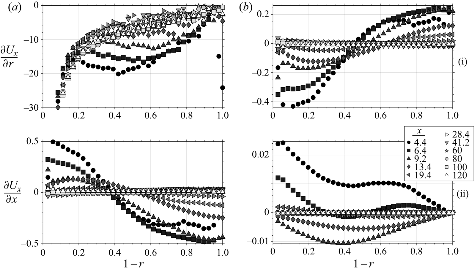
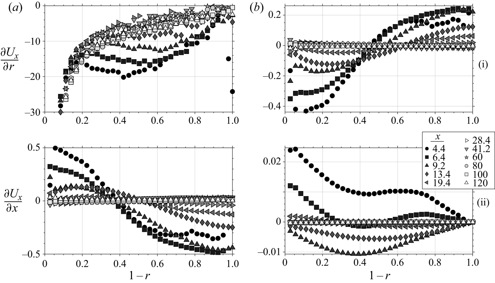
In figure 5 we compare the downstream development of the spatial gradients of the mean streamwise and wall-normal velocities. As was shown above (figure 3), the change in surface roughness causes an acceleration near the wall and a deceleration away from the wall. This streamwise gradient in  $U_x$ is necessarily coupled with a wall-normal gradient of
 $U_r$, where the streamwise acceleration near the wall and deceleration near the centre imply a positive radial velocity. Despite the non-equilibrium flow developing in the
 $x$ direction, the dominant spatial gradient is
 $\partial /\partial r$ for both components of velocity, where
 $\partial U_x/\partial r$ is at least two orders of magnitude larger than any other gradient.
Mean velocity spatial gradient profiles as they develop downstream.
The streamwise Reynolds-averaged momentum equation is given by
 \begin{equation} U_x \frac{\partial U_x}{\partial x} + U_r \frac{\partial U_x}{\partial r} = -\frac{\partial P}{\partial x} + \frac{1}{Re_\tau} \nabla^2\, U_x - \frac{\partial \overline{u_x^2}}{\partial x} - \frac{1}{r}\frac{\partial\, \overline{r u_x u_r}}{\partial r}, \end{equation}
where the Reynolds stresses  $R_{ij} = \overline {u_i u_j}$,
 $Re_\tau = u_{\tau _0} R/\nu$ and
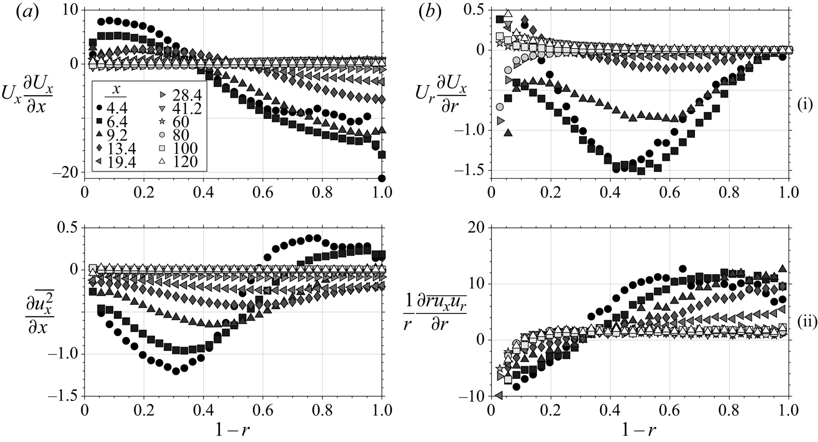
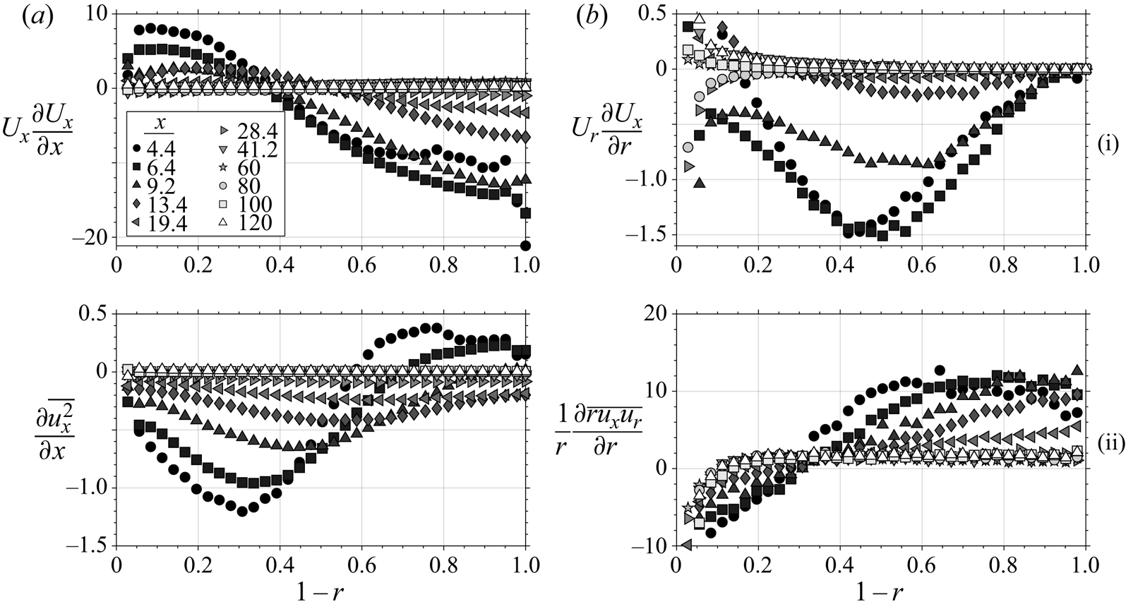
 $\nu$ is the kinematic viscosity. When the pressure gradient is constant (which happens relatively quickly as seen in figure 2), the major contributing terms in (3.2) are the convection (left-hand side) and the gradients of Reynolds stress, shown in figure 6. The streamwise development of
 $U_x$ (figure 6a-i) is primarily governed by the wall-normal gradient of the Reynolds shear stress
 $({1}/{r})({\partial \, \overline {r u_x u_r}}/{\partial r})$ (figure 6b-ii), and the remaining terms are small by comparison.
Transport (i) and Reynolds stress gradients (ii) of Navier–Stokes (3.2).
To explore the development of the Reynolds stresses, particularly  $\overline {u_x u_r}$, we consider the governing transport equations. Following Moser & Moin (Reference Moser and Moin1984), we interpret the transport of Reynolds stress as a balance of production, turbulent diffusion, pressure diffusion, viscous diffusion, pressure strain and viscous dissipation. That is,
 \begin{equation} \frac{\text{D} R_{ij}}{\text{D} t} = \underbrace{P_{ij}}_{\text{Production}} + \underbrace{TD_{ij}}_{\text{Turbulent diffusion}} + \underbrace{PD_{ij}}_{\text{Pressure diffusion}} + \underbrace{PS_{ij}}_{\text{Pressure strain}} + \underbrace{\frac{1}{Re_\tau}VD_{ij}}_{\text{Viscous diffusion}} + \underbrace{\frac{1}{Re_\tau}D_{ij}}_{\text{Viscous dissipation}}. \end{equation}
Here, we focus on the primary shear stress term ( $R_{xr}$) while the three normal stresses (
 $R_{xx}$,
 $R_{rr}$,
 $R_{\theta \theta }$) are relegated to the appendix A. The terms in (3.3) for
 $R_{xr}$ expand to
 \begin{equation} \left. \begin{array}{@{}c@{}} \displaystyle\frac{\text{D} R_{xr}}{\text{D} t} = U_x \frac{\partial\,\overline{u_x u_r}}{\partial x} + U_r \frac{\partial\,\overline{u_x u_r}}{\partial r},\\ \displaystyle P_{xr} = - \overline{u_r^2}\,\frac{\partial U_x}{\partial r} - \overline{u_x^2}\,\frac{\partial U_r}{\partial x} + \overline{u_r u_x}\,\frac{U_r}{r},\\ \displaystyle TD_{xr} = -\frac{1}{r}\frac{\partial}{\partial r}(r\overline{u_r^2u_x}) + \frac{1}{r}(\overline{u_\theta^2 u_x}) - \frac{\partial}{\partial x}(\overline{u_r u_x^2}),\\ \displaystyle PD_{xr} = -\frac{1}{r} \left(\frac{\partial \overline{r u_x p}}{\partial r}-\overline{u_x p}\right) - \frac{\partial \overline{u_r p}}{\partial x},\\ \displaystyle PS_{xr} = \overline{p \left(\frac{\partial u_x}{\partial r} + \frac{\partial u_r}{\partial x}\right) },\\ \displaystyle VD_{xr} = \frac{1}{r}\frac{\partial}{\partial r}\left( r\frac{\partial \overline{u_x u_r}}{\partial r} \right) + \frac{1}{r^2}\overline{u_x u_r} + \frac{\partial^2 \overline{u_x u_r}}{\partial x^2},\\ \displaystyle D_{xr} = - \overline{\frac{\partial u_r}{\partial x}\frac{\partial u_\theta}{\partial x}} - \overline{\frac{\partial u_r}{\partial r}\frac{\partial u_x}{\partial r}} - \overline{\left(\frac{1}{r}\frac{\partial u_r}{\partial \theta} - \frac{u_\theta}{r}\right) \frac{1}{r}\frac{\partial u_x}{\partial \theta}}. \end{array} \right\} \end{equation}
We will need to model the pressure terms ( $PD_{ij}$ and
 $PS_{ij}$ of (3.3)), because we do not have measurements of the fluctuating pressure, and the viscous dissipation terms (
 $D_{ij}$ of (3.3)), because we cannot properly resolve dissipation scales.
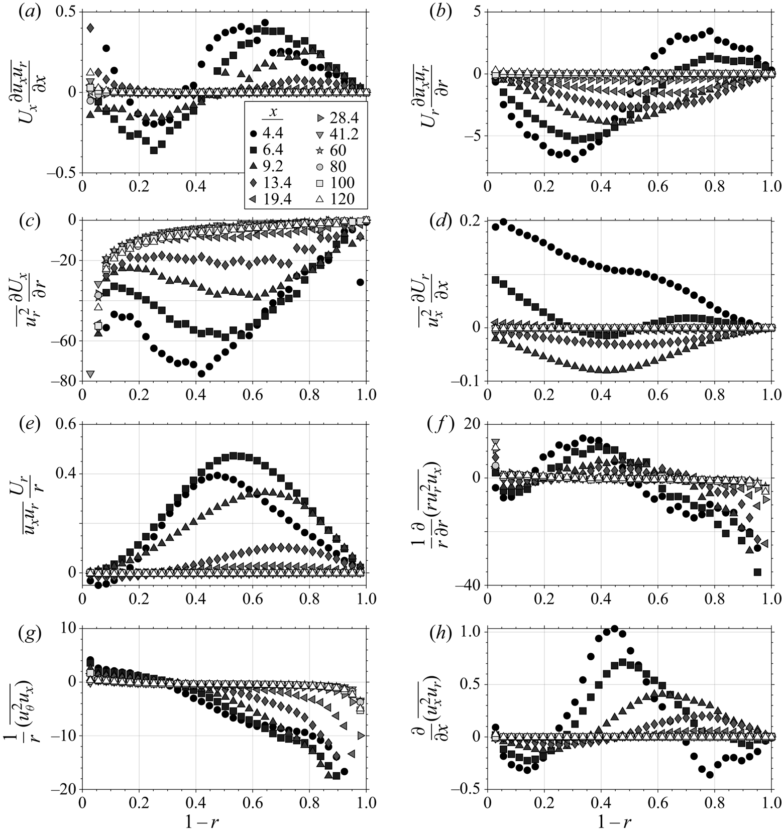
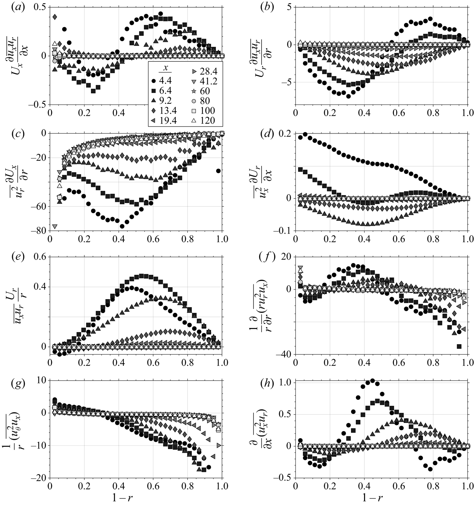
The other terms in (3.3) are shown in figure 7 for all downstream locations. Generally, the convection terms are small compared to the size of the production and turbulent diffusion terms. Specifically, the term 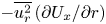 $- \overline {u_r^2}\,({\partial U_x}/{\partial r})$ (figure 7c), which acts as a source of
 $\overline {u_x u_r}$, is by far the largest and is likely balanced by the missing pressure strain term which acts to redistribute the turbulence and make the flow more isotropic, thus being a sink of
 $\overline {u_x u_r}$. Note that in fully developed channel flow, the production is almost completely balanced by the pressure strain away from the wall (Lee & Moser Reference Lee and Moser2015). The three turbulent diffusion terms can be meaningful near the step location, but they decay quickly and mostly cancel one another out, especially toward the pipe centre.
Transport (a,b), production (c–e) and turbulent diffusion (f–h) terms in the transport of  $\overline {u_x u_r}$ (3.3).
Finally, if we sum the transport of the normal Reynolds stresses  $R_{xx}$,
 $R_{rr}$ and
 $R_{\theta \theta }$ (the details are given in the appendix A), we arrive at the transport equation for turbulence kinetic energy
 $K$:
 \begin{align} &U_x \frac{\partial\,K}{\partial x} + U_r \frac{\partial\,K}{\partial r} = - \overline{u_x^2}\,\frac{\partial U_x}{\partial x}-\,\overline{u_r u_x}\,\frac{\partial U_x}{\partial r} -\,\overline{u_r^2}\,\frac{\partial U_r}{\partial r}-\,\overline{u_r u_x}\,\frac{\partial U_r}{\partial x} -\frac{1}{r}\overline{u_\theta^2}U_r\nonumber\\ &\quad - \frac{1}{2r}\frac{\partial}{\partial r}\left( r\overline{u_r u_x^2} - r\overline{u_r^3} - r\overline{u_ru_\theta^2}\right) - \frac{1}{2}\frac{\partial}{\partial x}\left( \overline{u_x^3} - \overline{u_r^2 u_x} - \overline{u_\theta^2 u_x}\right) + \frac{1}{Re_\tau}\nabla^2 K + \ldots , \end{align}
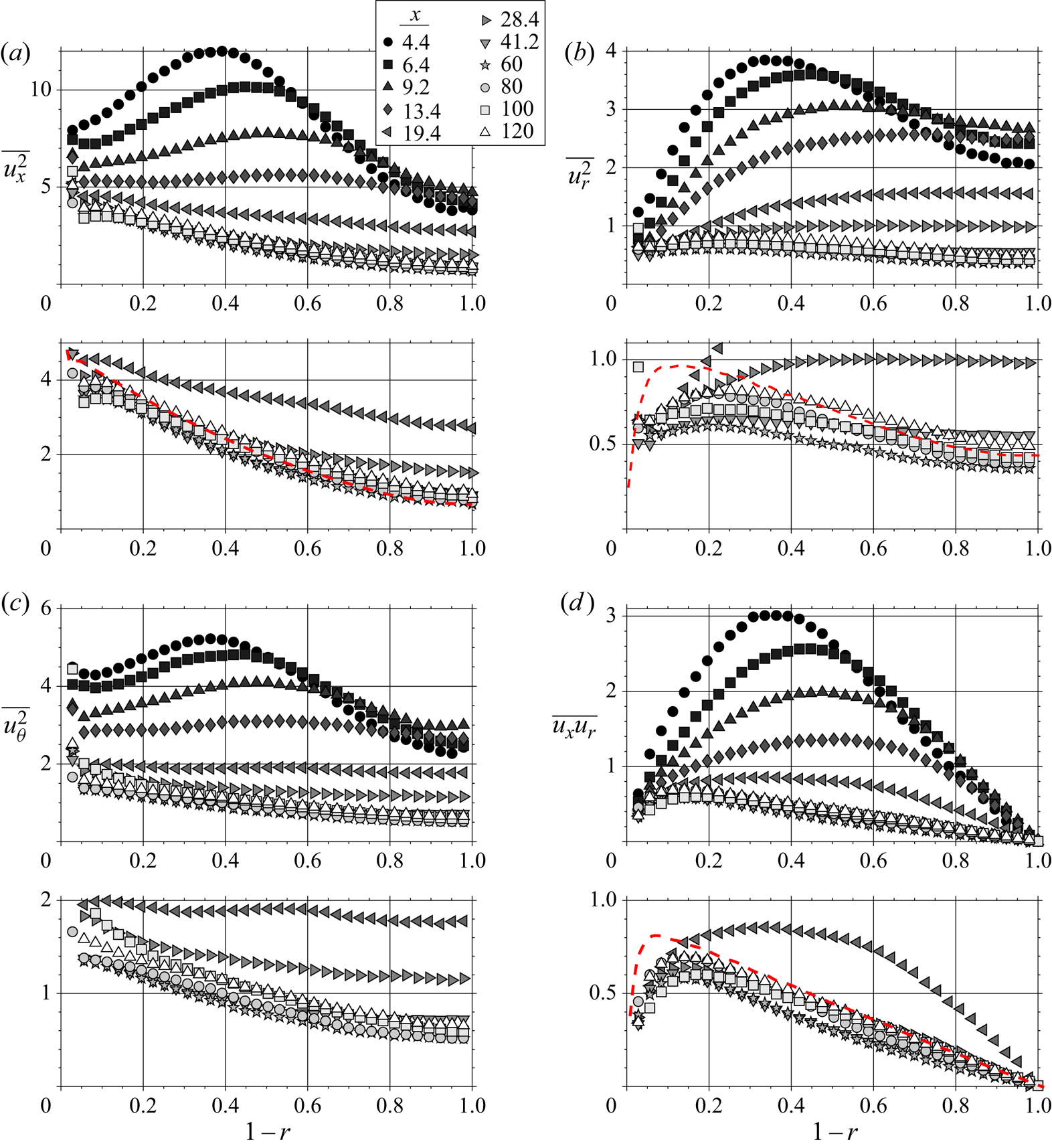
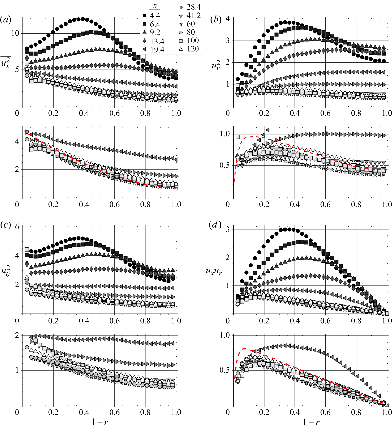
where we show only the contributions from production, turbulent diffusion and viscous diffusion, while the other terms are bundled in the ellipsis. The experimental results for the individual components of the turbulence kinetic energy and the primary Reynolds shear stress are shown in figure 8. All the stresses show similar trends, where the location nearest the step shows some peak in stress near a wall-normal location of 0.4 that gradually decays and broadens downstream. This peak occurs because the turbulence first responds near the wall and then moves toward the centre, thus creating a peak in the outer flow that moves away from the wall with distance downstream (most clearly seen in figure 8d). All the stresses then overshoot their expected values (shown by the red dashed line), and spend a considerable distance (almost  $100R$) with relatively low turbulence. Even at
 $120R$ downstream, the flow has not yet reached equilibrium. This trend is most exaggerated in
 $\overline {u_r^2}$ and
 $\overline {u_x u_r}$ (figure 8b,d), which indicates that the culprit for the overshoot may be the wall-normal velocity component. Note that the reference data were taken in the same facility with a completely smooth pipe, but with approximately twice the magnification and resolution compared to the current data.
Streamwise development of the Reynolds stresses  $\overline {u_x^2}$
 $(a)$,
 $\overline {u_r^2}$
 $(b)$,
 $\overline {u_\theta ^2}$
 $(c)$ and
 $\overline {u_x u_r}$
 $(d)$. Red dashed lines indicate expected asymptotic values of a data set taken with a completely smooth pipe.
Near the pipe centreline, the normal Reynolds stresses (figure 8a–c) initially increase downstream. It is well known that adverse pressure gradients enhance turbulence (Harun et al. Reference Harun, Monty, Mathis and Marusic2013), and the mechanism is obvious from an inspection of the  $K$ transport (3.5). The production term
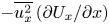 $-\overline {u_x^2}\,({\partial U_x}/{\partial x})$ is positive when the flow decelerates, and there are no other terms to balance. Thus, the immediate response of the centreline mean velocity to the step change – due to continuity – results in an immediate additional production of
 $K$, causing the normal Reynolds stresses to locally increase. The Reynolds shear stress
 $\overline {u_x u_r}$ does not behave this way because its production (3.4) does not have a
 ${\partial U_x}/{\partial x}$ term, and it also has pressure strain terms that similarly react to mean gradients which could balance any immediate reaction.
3.2. Estimating the recovery behaviour
3.2.1. Rough estimate
As the flow exits the rough pipe and adapts to the smooth-wall condition, it needs to dissipate a large amount of excess turbulence kinetic energy  $\Delta K$. To make an initial estimate of the distance
 $X_r$ over which this recovery takes place, we assume that the excess turbulence dissipates at a constant rate
 $\epsilon _0$. Hence,
 $X_r=(\Delta K/\epsilon _0)(U_b/R)$. The downstream development will be a function of wall-normal location, given that
 $\Delta K$ and
 $\epsilon _0$ both have wall-normal dependence.
Lower and upper bounds for  $X_r$ are given by using either the rough-wall dissipation rate or the smooth-wall dissipation rate. These dissipation rates were estimated using direct numerical simulations of turbulent channel flow at
 $Re_\tau =5200$ (Lee & Moser Reference Lee and Moser2015), and scaling them with
 $u_{\tau _r}$ and
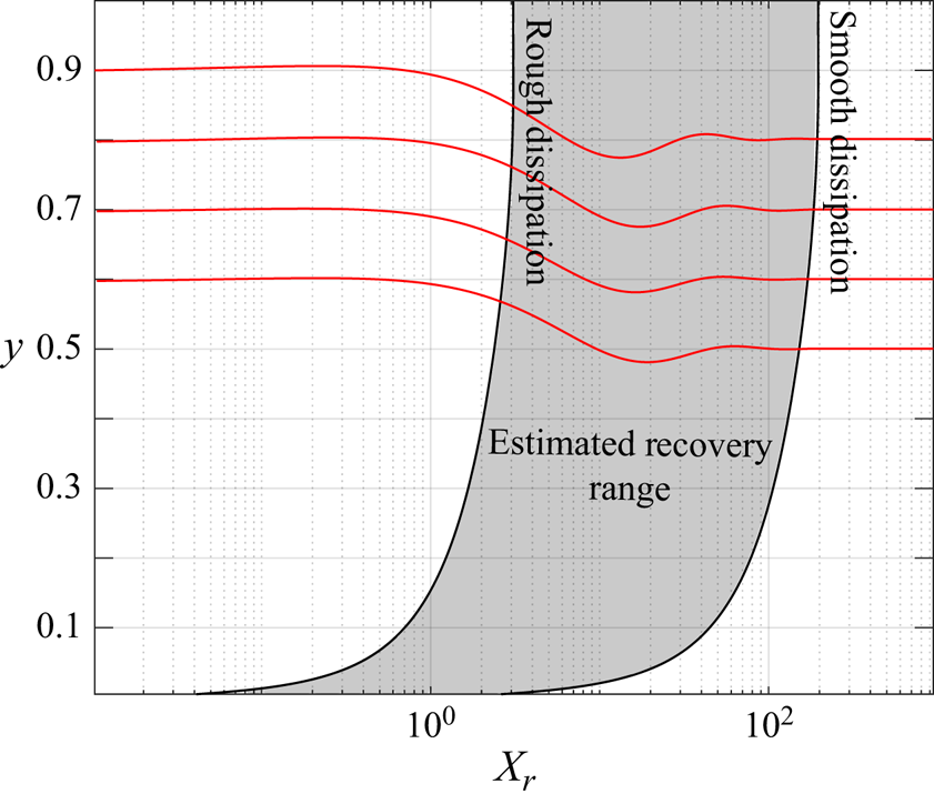
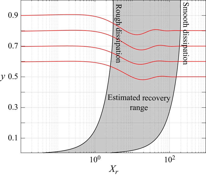
 $u_{\tau _0}$, respectively. Figure 9 shows these estimates which depend on the wall-normal location. The flow near the wall recovers much faster than the flow in the outer region, so the overall flow recovery will be set by the slow response of the outer region. If the turbulence dissipates at the rate given by the rough-wall condition throughout the entire development region,
 $X_r\approx 3$. If it were to recover at the smooth-wall condition throughout,
 $X_r \approx 200$. Both scenarios are unlikely, but these estimates show that we may expect relatively long recovery distances (
 $\mathcal {O}(100)$), due to the slow dissipation in the outer layer. Note that adding any level of turbulent production or wall-normal turbulent transport would only serve to slow the recovery even more.
Estimated recovery distance from a simplified scaling argument (shaded region). Solid red lines represent the relative streamwise development of a perturbation using response model (3.22) at four wall-normal locations (vertically offset by their wall-normal location).
3.2.2. Theoretical and data-driven model
To obtain better estimates for the recovery behaviour, we use a perturbation analysis inspired by Smits, Young & Bradshaw (Reference Smits, Young and Bradshaw1979), who considered the response of a flat-plate boundary layer subjected to the sudden onset of wall curvature. In our analysis, outside of the convective terms in the material derivative, we will neglect streamwise gradients ( $\partial (\cdot )/\partial x \approx 0$). As noted above, and as found by experiment (figures 5–7), changes in the streamwise direction are generally slow and transport is dominated by wall-normal gradients. We will also limit our analysis to the outer flow which should govern the rate of response, so we neglect the viscous stress gradients.
Under these conditions, the streamwise mean momentum (3.2) becomes
 \begin{equation} \frac{\text{D} U_x}{\text{D} t} = -\frac{\partial P}{\partial x} - \frac{1}{r}\frac{\partial\,r \tau}{\partial r}, \end{equation}
where  $\tau =\overline {u_x u_r}=R_{xr}$. We can remove the dependence on pressure by differentiating with respect to
 $r$, and by using continuity we obtain
 \begin{equation} \frac{\text{D}}{\text{D} t}\left(\frac{\partial U_x}{\partial r}\right) - \frac{U_r}{r}\frac{\partial U_x}{\partial r} = \frac{\tau}{r^2} - \frac{1}{r}\frac{\partial \tau}{\partial r} - \frac{\partial^2 \tau}{\partial r^2}. \end{equation}
Since the transport of  $\partial U_x / \partial r$ depends solely on the stress
 $\tau$, we need to consider the transport of stress (3.3),
 \begin{equation} \frac{\text{D} \tau}{\text{D} t} = - \overline{u_r^2}\,\frac{\partial U_x}{\partial r} + \overline{p \left(\frac{\partial u_x}{\partial r} + \frac{\partial u_r}{\partial x}\right)}, \end{equation}
assuming that turbulent and pressure diffusion are negligible in the outer layer (Lee & Moser Reference Lee and Moser2015), and that  $\partial U_r / \partial r\ll \partial U_x / \partial r$. That is, we retain only the contributions made by production and pressure strain.
The pressure strain (typically denoted by  $\varPi _{ij}$) is often modelled as the sum of a ‘slow’ and a ‘fast’ term (
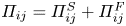 $\varPi _{ij} = \varPi _{ij}^S + \varPi _{ij}^F$), two terms that arise when the pressure fluctuations are presented in their exact integral form. The fast term interacts with the mean velocity gradient, thus responding instantly to a change in the mean flow, whereas the slow term relies only on turbulence quantities that are slower to change (Bernard & Wallace Reference Bernard and Wallace2002, § 2.3). We use the models presented by Rotta (Reference Rotta1951) and Crow (Reference Crow1968), where
 \begin{equation} \left. \begin{aligned} \varPi_{xr}^S & = -C_{_{PS}}^S\,\epsilon\, \frac{\tau}{2K},\\ \varPi_{xr}^F & = C_{_{PS}}^F K \frac{\partial U_x}{\partial r}. \end{aligned} \right\} \end{equation}
Note that the constants associated with pressure strain have a  $PS$ subscript. For the slow response term,
 $C_{_{PS}}^S$ is the Rotta constant (commonly
 $C_{_{PS}}^S=3$). For the fast-response pressure strain model
 $\varPi _{xr}^F$, we have applied a constant
 $C_{_{PS}}^F$ which will be tuned to match the fully developed simulation of Lee & Moser (Reference Lee and Moser2015). The dissipation is modelled by its isotropic estimate
 \begin{equation} \epsilon = \frac{K^{{3}/{2}}}{\mathcal{L}}, \end{equation}
where  $\mathcal {L}$ is a length scale similar to a mixing length normalized by the pipe radius. It is assumed to be relatively constant in the outer part of the flow. Substituting (3.9) and (3.10) to (3.8) results in
 \begin{equation} \frac{\text{D} \tau}{\text{D} t} = - \overline{u_r^2}\,\frac{\partial U_x}{\partial r} + C_{_{PS}}^F K \frac{\partial U_x}{\partial r} - \frac{C_{_{PS}}^S}{2 \mathcal{L}}K^{{1}/{2}}\tau. \end{equation}
We now consider perturbations in the mean velocity and stresses according to
 \begin{equation} \left. \begin{array}{@{}c@{}} \displaystyle U_x = U_{x,0} + \Delta U_x, \quad U_r = U_{r,0} + \Delta U_r, \quad \tau = \tau_0 + \Delta \tau,\\ \displaystyle \overline{u_x^2} = \overline{u_{x,0}^2} + C_x\Delta \tau, \quad \overline{u_r^2} = \overline{u_{r,0}^2} + C_r\Delta \tau, \quad \overline{u_\theta^2} = \overline{u_{\theta,0}^2} + C_\theta\Delta \tau, \end{array} \right\} \end{equation}
where terms with a subscript 0 denote the smooth-wall fully developed profiles (functions only of  $r$) and
 $\varDelta$ terms are modifications that also vary in the streamwise direction. We will assume that a disturbance in
 $R_{ii}$ takes the shape of the disturbance
 $R_{xr}$ such that
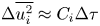 $\Delta \overline {u_i^2} \approx C_i\Delta \tau$ – a necessary assumption for this simplified analysis to work – and that the components differ only by some constant amplitude multiplier
 $C_i$. This assumption is justified to some extent by the similarities in the stress responses found by experiment, as shown in figure 8. Introducing these perturbations in (3.7) gives
 \begin{align} &(U_{x,0} + \Delta U_x)\frac{\partial}{\partial x}\left(\frac{\partial U_{x,0}}{\partial r} + \frac{\partial \Delta U_x}{\partial r} \right) + (U_{r,0} + \Delta U_r)\frac{\partial}{\partial r}\left(\frac{\partial U_{x,0}}{\partial r} + \frac{\partial \Delta U_x}{\partial r} \right)\nonumber\\ &\quad = \frac{1}{r^2}\frac{\partial r(\tau_0 + \Delta \tau)}{\partial r} - \frac{1}{r}\frac{\partial^2 r(\tau_0 + \Delta \tau)}{\partial r^2} + \frac{(U_{r,0} + \Delta U_r)}{r}\frac{\partial (U_{x,0} + \Delta U_x)}{\partial r}. \end{align}
Similarly, (3.8) becomes
 \begin{align} &(U_{x,0} + \Delta U_x)\frac{\partial (\tau_0 + \Delta \tau)}{\partial x} + (U_{r,0} + \Delta U_r)\frac{\partial (\tau_0 + \Delta \tau)}{\partial r}\nonumber\\ &\qquad = - (\overline{u_{r,0}^2} + C_r\Delta \tau)\,\frac{\partial (U_{x,0} + \Delta U_x)}{\partial r} + C_{_{PS}}^F K \frac{\partial (U_{x,0} + \Delta U_x)}{\partial r} - \frac{C_{_{PS}}^S}{2 \mathcal{L}}K^{{1}/{2}}(\tau_0 + \Delta \tau), \end{align}
where
 \begin{equation} K = \tfrac{1}{2}\left[\overline{u_{x,0}^2} + \overline{u_{r,0}^2} + \overline{u_{\theta,0}^2} + (C_x + C_r + C_\theta)\Delta \tau\right] = K_0 + \tfrac{1}{2}(C_x + C_r + C_\theta)\Delta \tau. \end{equation}
By definition,  $U_{r,0}=0$ and
 $\partial (\cdot )_0/\partial x = 0$, and all terms with only subscript 0 satisfy either (3.8) or (3.7) and can be removed. Linearizing removes
 $\Delta ^2$ terms, and then, by Taylor series expansion,
 $K^{{1}/{2}} \approx K_0^{{1}/{2}} + (K_0^{-{1}/{2}}(C_x + C_r + C_\theta )\Delta \tau )/4$ and
 $K^{{3}/{2}} \approx K_0^{{3}/{2}} + 3(K _0^{{1}/{2}}(C_x + C_r + C_\theta )\Delta \tau )/4$. Thus,
 \begin{equation} U_{x,0}\frac{\partial^2 \Delta U_x}{\partial x \partial r} + \Delta U_r\frac{\text{d}^2 U_{x,0}}{\text{d} r^2} = \frac{\Delta \tau}{r^2} - \frac{1}{r}\frac{\partial \Delta \tau}{\partial r} - \frac{\partial^2 \Delta \tau}{\partial r^2} + \frac{\Delta U_r}{r}\frac{\text{d} U_{x,0}}{\text{d} r}, \end{equation}
and
 \begin{align} U_{x,0}\frac{\partial
\Delta \tau}{\partial x} + \Delta U_r\frac{\text{d}
\tau_0}{\text{d} r} & =
-\overline{u_{r,0}^2} \frac{\partial \Delta U_x}{\partial
r} - C_r \frac{\text{d} U_{x,0}}{\text{d} r} \Delta \tau +
C_{_{PS}}^F K_0 \frac{\partial \Delta U_x}{\partial r} \notag\\ & \quad +
\frac{C_{_{PS}}^F}{2}(C_x + C_r + C_\theta) \frac{\partial
U_{x,0}}{\partial r} \Delta \tau\nonumber\\ &\quad
-\frac{C_{_{PS}}^S}{2 \mathcal{L}}\left[K_0^{{1}/{2}} +
\frac{1}{4}K_0^{-{1}/{2}}(C_x + C_r +
C_\theta)\tau_0\right]\Delta \tau.
\end{align}
We can make some additional approximations. In the outer region of turbulent pipe flow, the mean streamwise velocity curvature  $\partial ^2 U_{x,0}/\partial r^2$ is nearly zero and will be neglected. Second, by continuity, terms convected by
 $\Delta U_x$ are much larger than terms convected by
 $\Delta U_r$, so the latter terms can be ignored (see also figure 5). With these simplifications, we are left with
 \begin{equation} U_{x,0}\frac{\partial^2 \Delta U_x}{\partial x \partial r} = \frac{\Delta \tau}{r^2} - \frac{1}{r}\frac{\partial \Delta \tau}{\partial r} - \frac{\partial^2 \Delta \tau}{\partial r^2}, \end{equation}
and
 \begin{align} U_{x,0}\frac{\partial \Delta \tau}{\partial x} &= - \overline{u_{r,0}^2} \frac{\partial \Delta U_x}{\partial r} - C_r \frac{\text{d} U_{x,0}}{\text{d} r} \Delta \tau + C_{_{PS}}^F K_0 \frac{\partial \Delta U_x}{\partial r} \nonumber\\ &\quad + \frac{C_{_{PS}}^F}{2}(C_x + C_r + C_\theta) \frac{\partial U_{x,0}}{\partial r} \Delta \tau \nonumber\\ &\quad - \frac{C_{_{PS}}^S}{2 \mathcal{L}}\left[K_0^{{1}/{2}} + \frac{1}{4}K_0^{-{1}/{2}}(C_x + C_r + C_\theta)\tau_0\right]\Delta \tau. \end{align}
Following Smits et al. (Reference Smits, Young and Bradshaw1979), we break  $\Delta \tau$ into a product of separate functions of
 $x$ and
 $r$, i.e.
 $\Delta \tau (x,r) = \mathcal {T}(x) f(r)$. Unlike Smits et al. (Reference Smits, Young and Bradshaw1979), we will not require the disturbance to take the same wall-normal shape as
 $\tau _0$, which is a poor assumption according to the results given in figure 8. We then arrive at the final form of the mean-momentum equation, where
 \begin{equation} \frac{\partial}{\partial x}\left(\frac{\partial \Delta U_x}{\partial r}\right) = \frac{\mathcal{T}}{U_{x,0}}\left(\frac{f}{r^2} - \frac{1}{r}\frac{\partial f}{\partial r} -\frac{\partial^2 f}{\partial r^2}\right), \end{equation}
and the Reynolds stress transport equation,
 \begin{align} \frac{\partial\mathcal{T}}{\partial x} &= -\left(\overline{u_{r,0}^2} - C_{_{PS}}^F K_0 \right)\frac{1}{f \kern0.05em U_{x,0}} \frac{\partial \Delta U_x}{\partial r} - \frac{\mathcal{T} }{U_{x,0}} \left\{C_r \frac{\partial U_{x,0}}{\partial r} - \frac{C_{_{PS}}^F}{2}(C_x + C_r + C_\theta)\frac{\partial U_{x,0}}{\partial r}\right.\nonumber\\ &\left.\quad + \frac{C_{_{PS}}^S}{2 \mathcal{L}}\left[K_0^{{1}/{2}} + \frac{1}{4}K_0^{-{1}/{2}}(C_x + C_r + C_\theta)\tau_0 \right] \right\}. \end{align}
Combining (3.21) and (3.20) to remove the dependence on  $\mathcal {T}$, we come to
 \begin{align} &\ddot{\mathrm{X}} + \left\{ C_r U_{x,0}' - \frac{C_{_{PS}}^F}{2}C_{tot} U_{x,0}' + \frac{C_{_{PS}}^S}{2 \mathcal{L}}\left[K_0^{{1}/{2}} + \frac{1}{4}K_0^{-{1}{2}}C_{tot}\tau_0\right] \right\} \frac{1}{U_{x,0}} \dot{\mathrm{X}}\nonumber\\ &\quad + \left(\overline{u_{r,0}^2} - C_{_{PS}}^F K_0 \right)\left(\frac{f}{r^2} - \frac{f'}{r} - f'' \right)\frac{1}{f \kern0.05em U_{x,0}^2} \mathrm{X} = 0, \end{align}
where  $\mathrm {X} \equiv \partial \Delta U_x/\partial r$,
 $\dot {(\cdot )}$ denotes
 $\partial (\cdot )/\partial x$,
 $(\cdot )'$ denotes
 $\partial (\cdot )/\partial r$, and
 $C_{tot} = C_x + C_r + C_\theta$. Given an estimate for the wall-normal shape of the disturbance
 $f$, (3.22) is a solvable, ordinary second-order differential equation which takes the form of a damped simple harmonic oscillator.
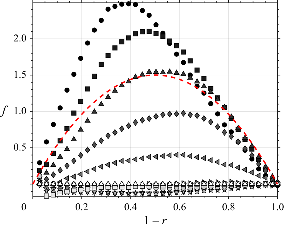
To approximate the disturbance, we assume a parabolic profile  $f = 1 - 4(r - 0.5)^2$. The constants in (3.22) were chosen so that
 $C_{_{PS}}^S = 3$ according to Bernard & Wallace (Reference Bernard and Wallace2002);
 $C_{_{PS}}^F=0.3$ to agree with the fully developed results from Lee & Moser (Reference Lee and Moser2015); and
 $C_x \approx 4$,
 $C_r \approx 1.2$ and
 $C_\theta \approx 1.6$, so that the Reynolds normal stresses are more impacted than the Reynolds shear stress in accordance with our measurements. The length scale
 $\mathcal {L}$ is approximated as
 $R$. For the terms with subscript 0, corresponding to the smooth-walled fully developed profiles, we use the channel flow results of Lee & Moser (Reference Lee and Moser2015).
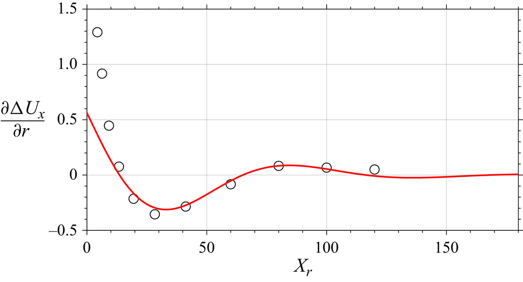
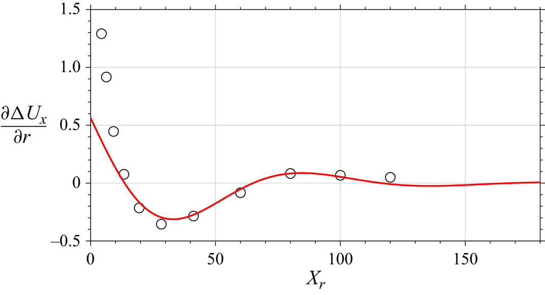
The responses given by this model are shown in figure 9 for four wall-normal locations in the outer layer. The point at which a disturbance has decayed, according to this model, occurs toward the higher end of the estimated recovery range, based on constant dissipation rates, indicating that the dissipation rate follows the smooth pipe value more closely than the rough pipe value. In figure 10, we see that the model compares well with the measurements of  $\partial \Delta U_x/\partial r$, averaged over the four wall-normal locations. There is particularly good agreement in the oscillation decay rate and wavelength, except for the region immediately downstream of the step where our assumptions are likely to be invalid (specifically that
 $\partial (\cdot )/\partial x \ll \partial (\cdot )/\partial r$).
Model (red solid line) from (3.22) compared to experimental measurements (circles) of  $\partial \Delta U_x/\partial r$, where the experiments are averaged over wall-normal locations
 $r = 0.4-0.7$ and the model is evaluated at that average wall-normal value.
The model can also be interpreted more physically. The coefficient on the term that dictates the rate of decay,  $\dot {\mathrm {X}}$, is primarily governed by the shape of the fully developed profiles (subscript 0) and the disturbance amplitudes; while the coefficient on the term that dictates the oscillation behaviour,
 $\mathrm {X}$, is the only one where the disturbance shape appears. Thus, the nature of the response is determined by the shape of the disturbance, so it will depend on the wall-normal location.
The choice of the disturbance shape and the assumptions regarding its behaviour are not trivial. Here, we have assumed the disturbance takes a parabolic shape, that it develops downstream by changing amplitude while preserving its shape, and that disturbances on all the Reynolds stresses behave similarly. In the appendix A, we show that, after the first few measurement locations, the disturbance profiles are close to being parabolic and that they remain that way through the rest of the domain (for the first few measurements the profiles are nearly parabolic but the peaks are not centred). The profiles shown in figure 8 also indicate that the disturbances are largely similar for each Reynolds stress – away from the pipe centre. Ultimately, it is the curvature of the disturbance shape that is important because it dictates the magnitude of  $f'$ and
 $f''$, which in turn determine the sign of the coefficient on
 $X$ in (3.22) and the oscillatory response condition. Whether the flow naturally converges to this disturbance profile or if it depends on the perturbation type (e.g. change in surface roughness, curvature, pipe area, etc.) is an open question.
A weakness of our model is that it is sensitive to the value of the empirical constants; changing almost any constant by  $\pm$20 % will result in a noticeable change in response behaviour. So, although the model works well here, using more-or-less reasonable choices for the constants and disturbance inputs, its broader use may be somewhat limited. Nevertheless, the analysis indicates that the oscillatory, slow-decay response of wall-bounded turbulent flows subject to perturbation is implicit in the governing equations, through the terms that describe the turbulence production and pressure strain.
3.3. Flow structure
To complement our analysis of the turbulence response in terms of the Reynolds-averaged equations, we now examine the response of the structure of turbulence in terms of a scale decomposition based on energy content. That is, we use proper orthogonal decomposition (POD) in the radial direction and Fourier decomposition in the azimuthal direction (the most energetic modes when there is azimuthal symmetry). For the Fourier decomposition,
 \begin{equation} u(r,\theta,t) = \sum_{m=-\infty}^\infty \hat{u}_m(r,t)\textrm{e}^{\textrm{i}\,m\theta}, \end{equation}
where  $m$ is the Fourier mode number. We can then organize the energy content by mode number to reveal the activity of structures of similar size.
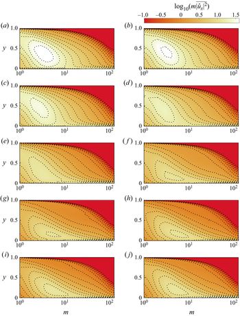
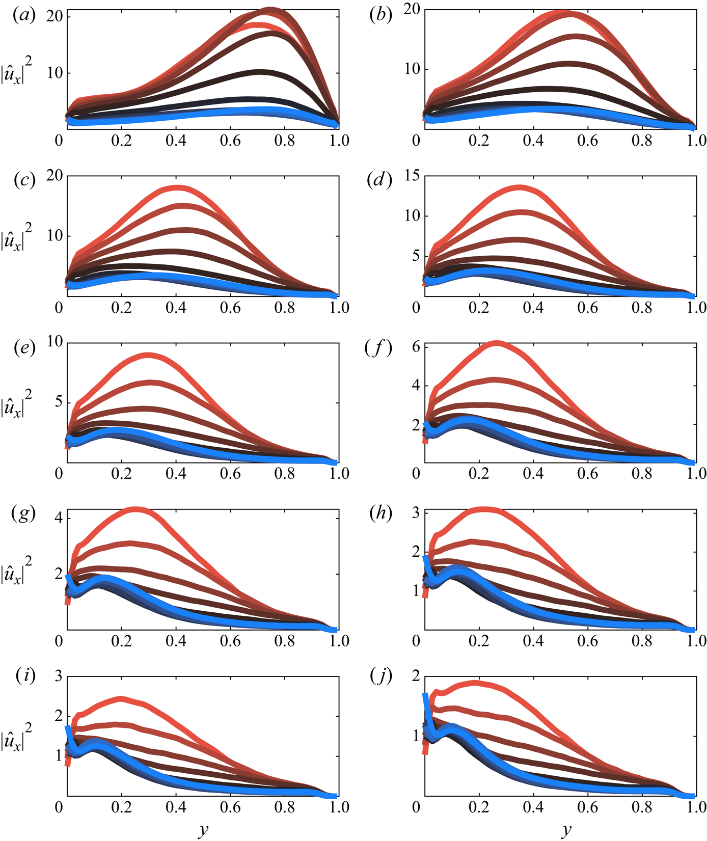
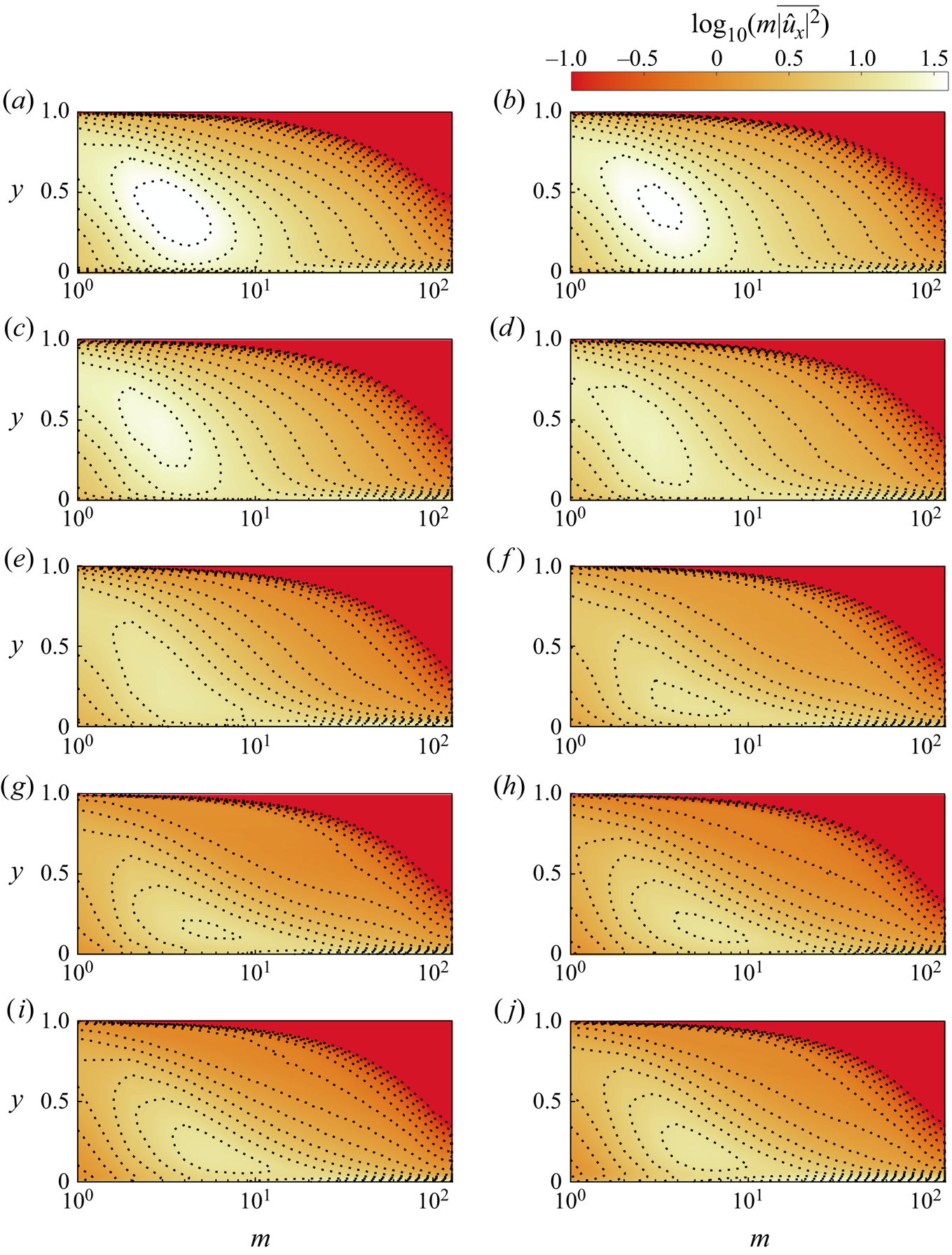
The contours of the premultiplied streamwise velocity spectra are shown in figure 11. Here, the vertical axis is the non-dimensional wall-normal location and the horizontal axis is the azimuthal mode number with logarithmic scaling. As the energy decays downstream the most energetic structures become smaller and move closer to the wall, with an overshoot similar to the one seen in the traditional statistics.
Premultiplied streamwise velocity power spectral density for downstream locations  $x=4.4\hbox{--}100$ (a–j).
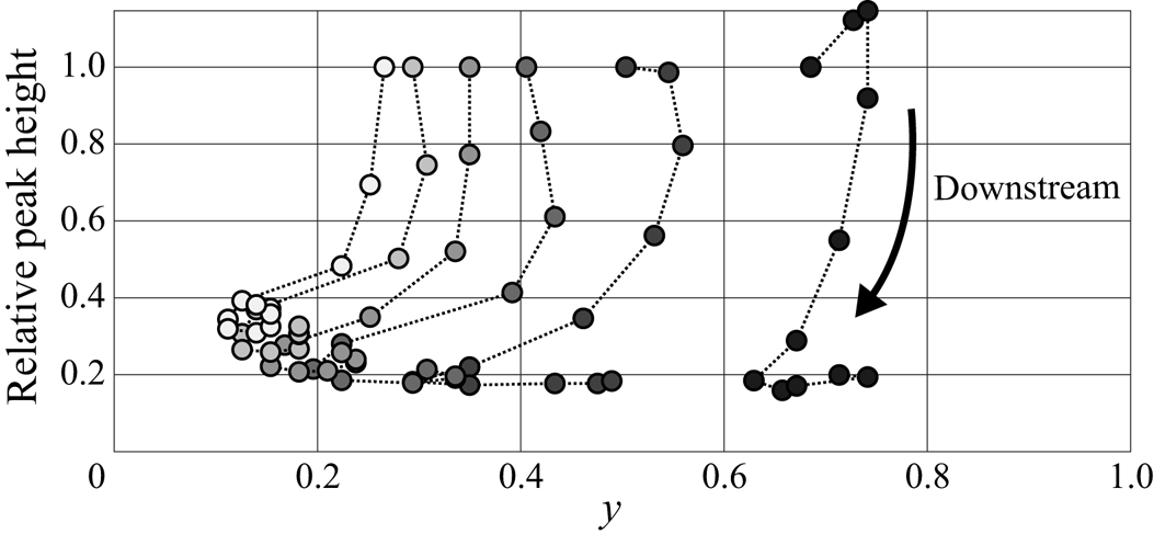
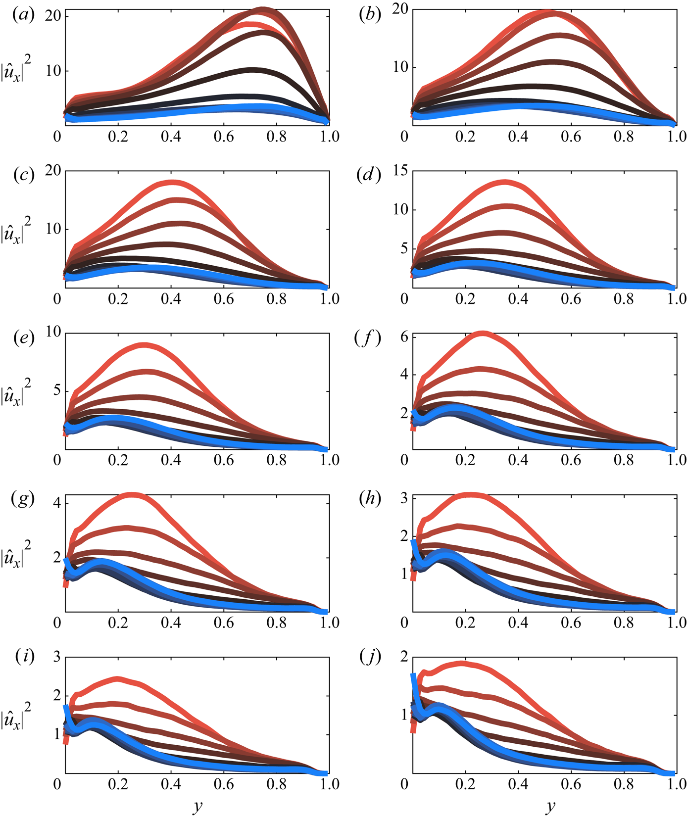
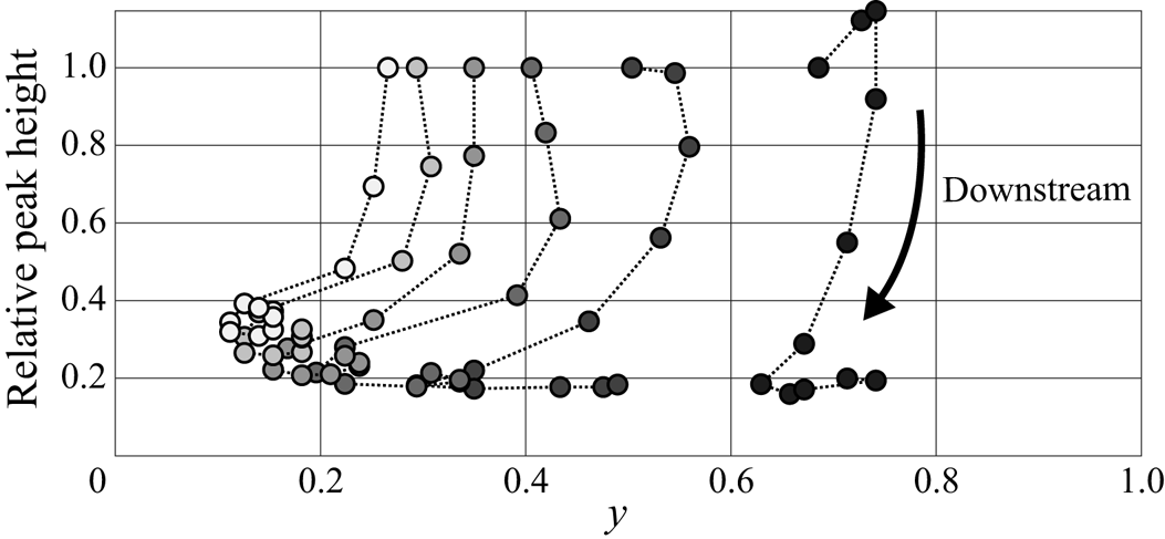
The individual mode profiles are in figure 12, where modes  $m=1\hbox{--}10$ are compared at all downstream locations, and the corresponding downstream development of the peaks for each profile are plotted in figure 13. We see that the largest structures (smallest mode number) are the slowest to respond which is consistent with our expectations (Li et al. Reference Li, de Silva, Rouhi, Baidya, Chung, Marusic and Hutchins2019). These large structures initially actually increase in energy before decaying, which may be driven by continuity through the immediate change in mean velocity gradients. (Alternatively, the modes corresponding to smaller structures may also initially increase before decaying in energy downstream of the step and our first measurement location is too far downstream to capture it.) For all modes, the peaks lose energy and gradually move towards the wall, and at some point further downstream, the modes start to move back away from the wall while keeping the same energy.
Streamwise velocity mode profiles for azimuthal modes  $m=1\hbox{--}10$ (a–j) and downstream locations
 $x=4.4\hbox{--}120$ (red to blue coloured lines, respectively).
Downstream development of the streamwise velocity mode peak location, relative to the first measurement location, for azimuthal modes  $m=1\hbox{--}6$ (black to white shaded symbols).
To gain insight about the different radial structures for a given azimuthal mode, we can further decompose the flow by applying POD to the radial direction, that is,
 \begin{equation} \hat{u}_m(r,t) = \sum_{n=1}^\infty c_{m,n}(t)\phi_{m,n}(r). \end{equation}
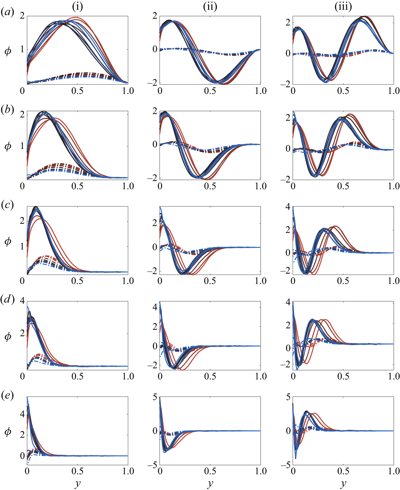
We expect that the radial mode shape  $\phi$ is closely tied to physical features in the flow, as previously demonstrated by Hellström, Sinha & Smits (Reference Hellström, Sinha and Smits2011) and Hellström & Smits (Reference Hellström and Smits2014).
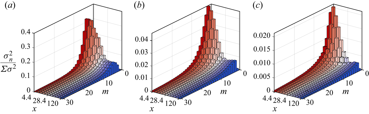
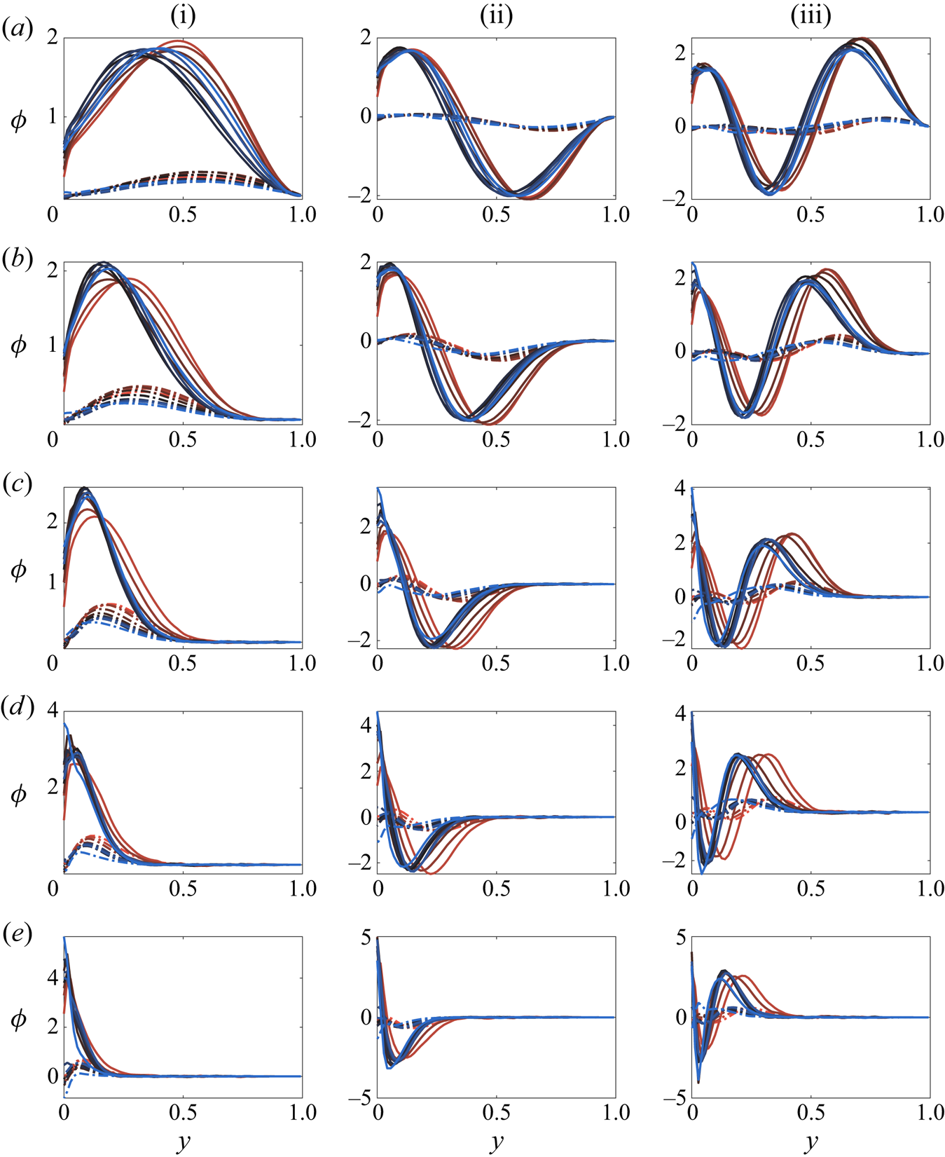
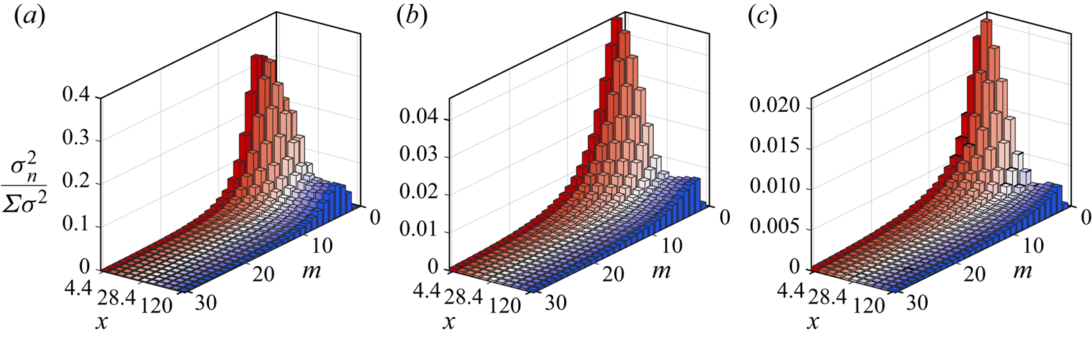
The radial mode profile shapes for the streamwise and wall-normal components are shown in figure 14. As they develop downstream (red to blue), the radial structures generally become more concentrated near the wall, however, the larger structures (e.g. figure 14a-i) first concentrate near the wall then exhibit a rebound, which may indicate that the rebounding of the turbulence statistics, seen in figure 8, is due primarily to the larger flow structures. Figure 15 shows the corresponding normalized POD mode energy for radial modes  $n=1\text{--}3$. Here we can more clearly see that the energy decays then rebounds most prominently in the largest structures, again reaffirming that the large structures are responsible for the second-order response. Remember that the model derived above, which accurately captures this second-order response, is a model for the outer flow which will likely be dominated by these larger structures, showing consistency between theory and experiment.
POD structure profiles for azimuthal modes  $m=3, 6, 12, 20, 30$ (a–e) and radial modes
 $n=1\hbox{--}3$ (i–iii), with both the streamwise and radial velocity component (solid and dashed lines). Downstream locations
 $x=4.4\hbox{--}120$ coloured red to blue.
Scaled azimuthal mode energy distribution for the radial modes  $n=1\hbox{--}3$ (a–c) development downstream
 $x=4.4\hbox{--}120$ (red to blue coloured bars).
4. Discussion and conclusions
Starting with fully developed pipe flow, we examined its response as the surface condition changed abruptly from rough to smooth. The flow over the entire cross-section of the pipe responds immediately to this step change due to mass conservation, where the acceleration near the wall must be balanced in an integral sense by the deceleration in the bulk of the flow. This feature distinguishes interior flows such as pipes and channels from exterior flows such as boundary layers.
In broad terms, however, the flow response is rather similar to that seen in studies of boundary layers experiencing comparable step changes. Global quantities like momentum gradient, pressure gradient, and skin friction recover within 20 $R$ downstream of the step, while the recovery of the turbulence is much slower. Even at the most downstream station, located
 $120R$ downstream (much farther than in previous studies of this kind), the departure from self-similarity in the stress response was still evident. Also, the relaxation of the turbulence was not monotonic but exhibited a second-order-like response behaviour, and for long distances, the bulk of the flow contained lower turbulence kinetic energy levels than those found in fully developed smooth-wall flow at the same Reynolds number. Such action has been observed in other flows as well, notably the recovery of a boundary layer from a short region of surface curvature (Smits et al. Reference Smits, Young and Bradshaw1979) and the response of channel flow to periodic rough-to-smooth transitions sees a similarly long recovery (Saito & Pullin Reference Saito and Pullin2014). It is also possible that this type of response exists in boundary layers experiencing a step change in roughness, but the existing data sets do not track the flow sufficiently far downstream to see the far-downstream behaviour (see, for example, Antonia & Luxton Reference Antonia and Luxton1971, Reference Antonia and Luxton1972).
To help understand this behaviour, we reviewed the governing equations and computed all the terms available from our measurements. The continuity equation indicated that the wall-normal gradient of the mean streamwise velocity ( $\partial U_x / \partial r$) continues to be the dominant term – as it is in fully developed flows. In turn, the Reynolds averaged Navier–Stokes equation showed that this gradient is governed principally by wall-normal gradients of the Reynolds shear stress (
 $({1}/{r})({\partial \overline {r u_x u_r} }/{\partial r})$).
The recovery behaviour was then studied by perturbing the Reynolds-averaged transport equations for the mean streamwise momentum and Reynolds shear stress. The model used simple estimates of the pressure strain and dissipation terms and assumed that the perturbations to Reynolds stress distributions all took the same shape (which the data showed was a plausible assumption). For the slow-to-respond outer flow, the model yielded a transport equation in the form of a damped harmonic oscillator. The solution matched our measurements reasonably well for  $x>10$, and successfully captured the second-order response. Because this model is generalized to consider a perturbation in the velocity field, it is possible that this type of response exists for other forms of perturbation (sudden change in area, curvature, etc.). In addition, further exploration of the model may indicate that this type of response also manifests itself in channels or boundary layers. (However, there are important differences between the governing equations in Cartesian and cylindrical coordinate systems, and the model would need to be fully re-assessed before implementation.)
Through data decomposition, we segregated the most energetic flow structures by size and found that all structures responded with similar characteristic development. Generally, the most energetic flow structures were seen to move towards the wall as they moved downstream, and as their characteristic wall-normal size decreased. Not surprisingly, the largest structures were the slowest to respond and are likely the primary source of the overshoot in flow response. Since the slow response is governed by the largest structures, models (like ours) that consider only the flow away from the wall – where these large structures dominate – may be a viable approach for describing the recovery behaviour in other flows that experience a sudden change in surface conditions. In particular, it appears that turbulent diffusion plays a rather limited role in determining recovery behaviour, which leads to useful simplifications in the turbulence modelling framework.
Acknowledgements
We gratefully acknowledge the support under ONR Grant ‘Understanding Turbulence on Navy Vehicles’ N00014-17-1-2309 (Program Manager J. Gorski).
Declaration of interests
The authors report no conflict of interest.
Appendix A
A.1. Uncertainty analysis
In particle image velocimetry (PIV) measurements, a velocity component  $\tilde {u}_m$ at a spatial location
 $\boldsymbol {x}$ and time
 $t$ can be decomposed into the true velocity
 $\tilde {u}$, a bias error
 $u_b$, and a random error
 $u_e$:
 \begin{equation} \tilde{u}_m(\boldsymbol{x},t) = \tilde{u}(\boldsymbol{x},t)+u_b(\boldsymbol{x},t)+u_e(\boldsymbol{x},t). \end{equation}
Note that  $u_b$ here is dependent on both
 $\boldsymbol {x}$ and
 $t$, as the bias error in PIV is usually correlated with local flow kinematics as a result of the finite interrogation volume. The random error
 $u_e$ typically stems from the randomness of particle distribution in an interrogation volume, the electronic noise of an image sensor, etc. We assume
 $u_e$ is a zero-mean random variable in both space and time.
With (A 1), we can derive different errors encountered in turbulence measurements with PIV. Averaging (A 1) in time yields
 \begin{equation} U_m = U+\overline{u_b}, \end{equation}
wherein the over bar indicates a time average, and  $U$ =
 $\overline {\tilde {u}}$ and
 $U_m = \overline {\tilde {u}_m}$ are the true and measured mean velocities, respectively;
 $\overline {u_b}$ is the time-invariant part of the bias error due to, e.g. optical distortion, calibration, non-uniform illumination, etc. This type of bias is usually insignificant in carefully conducted experiments. What requires more attention is the bias error in the estimation of Reynolds stresses. Subtracting (A 2) from (A 1) gives an estimate of the fluctuating velocity
 \begin{equation} u_m = u+(u_b-\overline{u_b})+u_e, \end{equation}
wherein  $u$ and
 $u_m$ denote the true and measured fluctuating velocities, respectively;
 $(u_b-\overline {u_b})$ is the part of bias error that is correlated with local flow kinematics. Given that PIV low-pass filters turbulent fields and thus tends to underestimate fluctuations, it is safe to conjecture
 $(u_b-\overline {u_b}) = -\alpha u$ with
 $0<\alpha <1$, that is,
 $(u_b-\overline {u_b})$ is negatively correlated with
 $u$. Equation (A 3) then becomes
 \begin{equation} u_m = (1-\alpha)u+u_e, \end{equation}
from which we can derive the turbulence intensity
 \begin{equation} \overline{u^2}_m= A_{11}\overline{u^2}+\overline{u^2_e}, \end{equation}
and the Reynolds shear stress
 \begin{equation} \overline{uv}_m = A_{12}\overline{uv}. \end{equation}
Here,  $A_{1}$,
 $A_{12} \in (0,1)$ are factors characterizing unresolved turbulent motions. The derivations of (A 5) and (A 6) use the assumption that
 $u_e$ and
 $v_e$ are uncorrelated and they are uncorrelated with
 $u$ and
 $v$. Now it becomes evident that PIV underestimates Reynolds stresses at an insufficient spatial resolution. Also, the random error
 $u_e$ contributes a positive bias in the estimation of turbulence intensity but not the Reynolds shear stress since
 $\overline {u_e v_e} = 0$.
Spatial attenuation is a well-known and long-standing limitation of PIV in turbulence studies (Kähler, Scharnowski & Cierpka Reference Kähler, Scharnowski and Cierpka2012; Scharnowski, Hain & Kähler Reference Scharnowski, Hain and Kähler2012). The unresolved turbulent energy is difficult to be quantified without fully resolved data. Some correction schemes have gained success in correcting turbulence statistics in canonical flows (Segalini et al. Reference Segalini, Bellani, Sardina, Brandt and Variano2014; Lee, Monty & Hutchins Reference Lee, Monty and Hutchins2016), but no universal methods exist for strongly disturbed, non-equilibrium flows.
While correction of attenuated Reynolds stresses is beyond the scope of this work, it is possible and necessary to examine the effect of  $\overline {u_e^2}$ on the convergence of turbulence statistics. To evaluate
 $\overline {u_e^2}$, we adopt the method described in Adrian & Westerweel (Reference Adrian and Westerweel2011, § 9.4.5) that makes use of the assumption that
 $u_e$ from different spatial locations are uncorrelated. Use (A 4) to express the two-point correlation function
 \begin{equation} R_{11}(\Delta r)_m = \overline{u_m(x)u_m(x+\Delta r)} = A_{\Delta r}\overline{u(x)u(x+\Delta r)}+\overline{u_e(x)u_e(x+\Delta r)}, \end{equation}
with  $A_{\Delta r}\in (0,1)$. Given that
 $\overline {u_e(x)u_e(x+\Delta r)} = 0$ when
 $\Delta r \neq 0$, an estimate of
 $\overline {u^2}$ free of random error is obtained
 \begin{equation} \overline{u^2} \approx \lim_{\Delta r \to 0}R_{11}(\Delta r)_m = \overline{u^2}_m-\overline{u_e^2}. \end{equation}
Equation (A 8) suggests that the difference between the directly measured turbulence intensity,  $\overline {u^2}_m$, and the extrapolation of
 $R_{11}(\Delta r)_m$ at
 $\Delta r = 0$ is an estimate of
 $\overline {u_e^2}$. Practically, the extrapolation can be reliably calculated using the relation
 $R_{11}(\Delta r) \approx R_{11}(0)-\Delta r^2 R''_{11}(0)/2$ for small
 $\Delta r$ when the separation
 $\Delta r$ is along a homogeneous direction.
PIV data in a fully developed turbulent pipe flow at  $Re_\tau = 3760$ are used to examine
 $\overline {u_e^2}$. The data were taken in a streamwise–radial plane, and velocity vectors were computed with an interrogation spot size of 120 viscous units and 50 % window overlap. It is worth noting that this fully developed data set was acquired in the same pipe facility with the same camera and laser at a similar spatial resolution as the stereoscopic PIV data presented in the main body of this paper. Therefore, the
 $\overline {u_e^2}$ result presented in this appendix is representative of the uncertainty level of the stereoscopic PIV data.
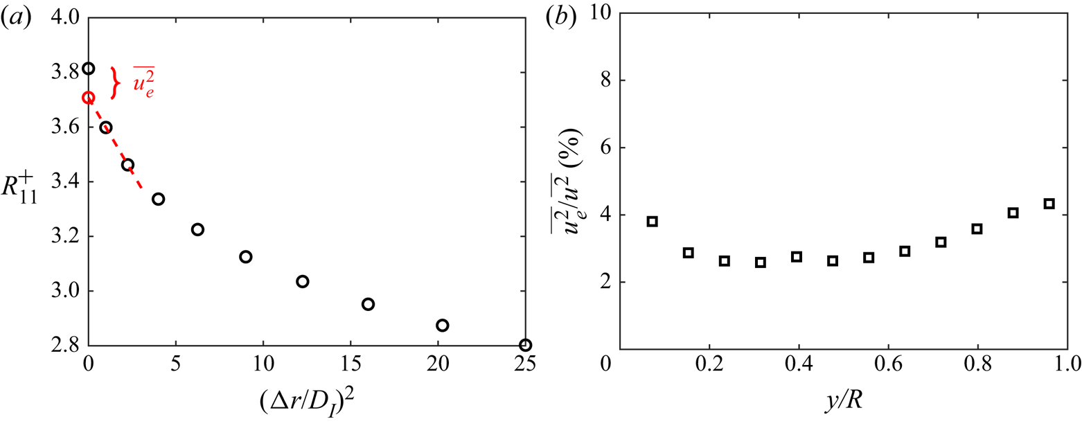
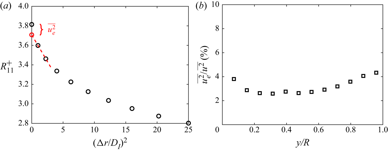
Figure 16 $(a)$ shows
 $R_{11}$ as a function of
 $(\Delta r/D_I)^2$ at
 $y/R \approx 0.15$, with
 $\Delta r$ in the streamwise direction. The red dashed line illustrates the extrapolation to
 $\Delta r = 0$, from which
 $\sqrt {\overline {u_e^2}}$ is estimated to be
 $0.06\ \textrm {m}\,\textrm {s}^{-1}$, corresponding to a displacement random error of 0.12 pixel in the image space. The displacement random error is found to decrease with
 $y/R$ from approximately 0.15 pixel to 0.05 pixel. The ratio of
 $\overline {u_e^2}$ to the local turbulence intensity is between 2 % and 4 % over
 $0< y/R <1$, which is plotted in figure 16
 $(b)$.
 $(a)$ Two-point correlation function
 $R_{11}$ (black circles) calculated from PIV data in a fully developed turbulent pipe flow.
 $R_{11}$ is plotted against
 $(\Delta r/D_I)^2$, where
 $\Delta r$ is the streamwise separation and
 $D_I$ is the interrogation spot size. The red dashed line is a linear fit to
 $R_{11} = R_{11}(0)-R^{''}_{11}(0)\Delta r^2/2$ using the second and third data points from the left. The red circle on the vertical axis indicates
 $R_{11}(0)$ projected from the fit. The discrepancy between the two estimates of
 $R_{11}(0) = \overline {u^2}$ is a measure of the variance of random error,
 $\overline {u_e^2}$.
 $(b)$ The ratio of
 $\overline {u_e^2}$ to the local turbulence intensity.
In view of  $\overline {u_e^2} \ll \overline {u^2}$, the convergence of turbulence statistics is dictated by turbulent fluctuations but not the random error. The standard deviations of the estimates of
 $U$,
 $\overline {u^2}$ and
 $\overline {uv}$ are given by
 \begin{gather} \sigma\left[U_m\right] = \frac{\overline{u^2}_m^{{1}/{2}}}{\sqrt{N_F}}, \end{gather}
 \begin{gather} \sigma\left[\overline{u^2}_m\right] = \frac{\sqrt{2}\,\overline{u^2}_m}{\sqrt{N_F}}, \end{gather}
and
 \begin{equation} \sigma\left[\overline{uv}_m\right] = \frac{(\overline{u^2}_m \overline{v^2}_m+\overline{uv}_m^2)^{{1}/{2}}}{\sqrt{N_F}}, \end{equation}
wherein  $N_F$ is the total number of independent frame pairs. In the PIV data presented in the main body,
 $\sqrt {N_F} \approx 100$, and
 $\overline {u_x^2}^{{1}/{2}}$ is as high as approximately 20 % of
 $U$. Therefore, according to (A 9), the standard deviation of
 $U$ is around 0.2 % of
 $U$, significantly lower than the changes between different
 $x$ locations (figures 3 and 10). Likewise, (A 10) implies that the fluctuation in the estimate of turbulent kinetic energy is around 1.4 %, noticeably smaller than the differences seen in figures 2 and 8 even at the last few
 $x$ locations. Regarding the fluctuation in
 $\overline {u_x u_r}$, if we approximate
 $\overline {u_x^2}:\overline {u_r^2}:\overline {u_x u_r} \approx 12:4:3$ based on the results in figure 8, then
 $\sigma [\overline {u_x u_r}]/\overline {u_x u_r} \approx 2.5\,\%$, also a small number as compared to the downstream evolution of
 $\overline {u_x u_r}$.
A.2. Transport equations
The terms in the  $R_{xx}$,
 $R_{rr}$ and
 $R_{\theta \theta }$ transport equation (3.3). First, the material derivative
 \begin{equation} \left. \begin{aligned} \frac{\text{D} R_{xx}}{\text{D} t} & = U_x \frac{\partial\,\overline{u_x^2}}{\partial x} + U_r \frac{\partial\,\overline{u_x^2}}{\partial r},\\ \frac{\text{D} R_{rr}}{\text{D} t} & = U_x \frac{\partial\,\overline{u_r^2}}{\partial x} + U_r \frac{\partial\,\overline{u_r^2}}{\partial r},\\ \frac{\text{D} R_{\theta \theta}}{\text{D} t} & = U_x \frac{\partial\,\overline{u_\theta^2}}{\partial x} + U_r \frac{\partial\,\overline{u_\theta^2}}{\partial r}. \end{aligned} \right\} \end{equation}
The production,
 \begin{equation} \left. \begin{array}{@{}c@{}} \displaystyle P_{xx} = -2\,\overline{u_x^2}\,\frac{\partial U_x}{\partial x}-2\,\overline{u_r u_x}\,\frac{\partial U_x}{\partial r},\\ \displaystyle P_{rr} = -2\,\overline{u_r^2}\,\frac{\partial U_r}{\partial r}-2\,\overline{u_r u_x}\,\frac{\partial U_r}{\partial x},\\ \displaystyle P_{\theta \theta} = -\frac{2}{r}\overline{u_\theta^2}U_r. \end{array} \right\} \end{equation}
The turbulent diffusion,
 \begin{equation} \left. \begin{array}{@{}c@{}} \displaystyle TD_{xx} = -\frac{1}{r}\frac{\partial}{\partial r}(r\overline{u_ru_x^2}) - \frac{\partial}{\partial x}(\overline{u_x^3}),\\ \displaystyle TD_{rr} = -\frac{1}{r}\frac{\partial}{\partial r}(r\overline{u_r^3}) + \frac{2}{r}(\overline{u_r u_\theta^2}) - \frac{\partial}{\partial x}(\overline{u_r^2 u_x}),\\ \displaystyle TD_{\theta \theta} = -\frac{1}{r}\frac{\partial}{\partial r}(r\overline{u_ru_\theta^2}) - \frac{2}{r}(\overline{u_r u_\theta^2}) - \frac{\partial}{\partial x}(\overline{u_\theta^2 u_x}). \end{array} \right\} \end{equation}
The pressure diffusion,
 \begin{equation} \left. \begin{array}{@{}c@{}} \displaystyle PD_{xx} = -2\frac{\partial \overline{u_x p}}{\partial x},\\ \displaystyle PD_{rr} = -\frac{2}{r}\left(\frac{\partial \overline{r u_r p}}{\partial r}-\overline{u_r p}\right),\\ \displaystyle PD_{\theta \theta} = -\frac{2}{r}\left(\frac{\partial \overline{u_\theta p}}{\partial \theta}+\overline{u_r p}\right). \end{array} \right\} \end{equation}
The pressure strain,
 \begin{equation} \left. \begin{array}{@{}c@{}} \displaystyle PS_{xx} = 2 \overline{p\frac{\partial u_x}{\partial x}},\\ \displaystyle PS_{rr} = 2 \overline{p\frac{\partial u_r}{\partial r}},\\ \displaystyle PS_{\theta \theta} = \frac{2}{r} \overline{p \left(\frac{\partial u_\theta}{\partial \theta} + u_r \right). } \end{array} \right\} \end{equation}
The viscous diffusion,
 \begin{equation} \left. \begin{array}{@{}c@{}} \displaystyle VD_{xx} = \frac{1}{r}\frac{\partial}{\partial r}\left( r\frac{\partial \overline{u_x^2}}{\partial r} \right) + \frac{\partial^2 \overline{u_x^2}}{\partial x^2}, \\ \displaystyle VD_{rr} = \frac{1}{r}\frac{\partial}{\partial r}\left( r\frac{\partial \overline{u_r^2}}{\partial r} \right) + \frac{2}{r^2}(\overline{u_\theta^2} - \overline{u_r^2}) + \frac{\partial^2 \overline{u_r^2}}{\partial x^2}, \\ \displaystyle VD_{\theta \theta} = \frac{1}{r}\frac{\partial}{\partial r}\left( r\frac{\partial \overline{u_\theta^2}}{\partial r} \right) - \frac{2}{r^2}(\overline{u_\theta^2} - \overline{u_r^2}) + \frac{\partial^2 \overline{u_\theta^2}}{\partial x^2}. \end{array} \right\} \end{equation}
Lastly, the viscous dissipation,
 \begin{equation} \left. \begin{array}{@{}c@{}} \displaystyle D_{xx} = - \overline{\left(\frac{\partial u_x}{\partial x}\right)^2} - \overline{\left(\frac{\partial u_x}{\partial r}\right)^2} - \overline{\left(\frac{1}{r}\frac{\partial u_x}{\partial \theta}\right)^2}, \\ \displaystyle D_{rr} = - \overline{\left(\frac{\partial u_r}{\partial x}\right)^2} - \overline{\left(\frac{\partial u_r}{\partial r}\right)^2} - \overline{\left(\frac{1}{r}\frac{\partial u_r}{\partial \theta} - \frac{u_\theta}{r}\right)^2}, \\ \displaystyle D_{\theta \theta} = - \overline{\left(\frac{\partial u_\theta}{\partial x}\right)^2} - \overline{\left(\frac{\partial u_\theta}{\partial r}\right)^2} - \overline{\left(\frac{1}{r}\frac{\partial u_\theta}{\partial \theta} + \frac{u_r}{r}\right)^2}. \end{array} \right\} \end{equation}
A.3. Disturbance profile
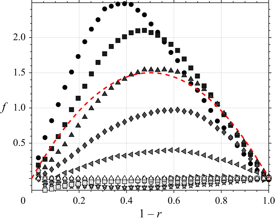
We check our assumption that a disturbance on  $\tau$ takes the approximate parabola with preserved shape downstream. Figure 17 shows the disturbance profiles of the measured
 $\overline {uv}$ data as they develop (here, to obtain the disturbance profile we have subtracted the final measurement location as an estimate of the unperturbed case). A representative parabola is also plotted for comparison.
Disturbance shape as it varies downstream (symbols as in figure 8) compared to a parabola (red dashed line).