1. Introduction
Magnetic islands are a well-studied phenomenon in plasma physics. They are the result of a change in the topology of the magnetic field following a reconnection process. The interest of the fusion community in this phenomenon is mostly due to the negative effects they have on the confinement properties of the plasma, and to the fact that they might lead to disruptions in tokamak discharges, thus potentially damaging the device they occur in.
With respect to the transport properties, one of the most prominent effects of magnetic islands is that, in general, they cause a flattening of the radial pressure profile inside the separatrix (i.e. the surface that separates the island from the rest of the plasma), thus limiting the maximum achievable pressure in the core, and, consequently, the performance of the plasma. The flattening is due to the nested magnetic flux surfaces that form inside the separatrix which encloses the island. On these flux surfaces, the plasma is free to stream with the high speeds of parallel motion in magnetic confinement devices, thus efficiently connecting two radially distant points, quickly eliminating the pressure gradient inside the separatrix (Fitzpatrick Reference Fitzpatrick1995). This flattening is, however, only effective if the width of the island crosses a critical threshold above which the parallel diffusion is more efficient than the perpendicular.
A flat pressure gradient is, in turn, reason for concern for the growth of so-called neoclassical tearing modes (NTMs Sauter et al. Reference Sauter, La Haye, Chang, Gates, Kamada, Zohm, Bondeson, Boucher, Callen and Chu1997), i.e. magnetic islands whose driving mechanism is the suppression of the bootstrap current linked to the fading pressure gradient (Carrera, Hazeltine & Kotschenreuther Reference Carrera, Hazeltine and Kotschenreuther1986; Reimerdes et al. Reference Reimerdes, Sauter, Goodman and Pochelon2002). This kind of island requires the presence of a seed island above a critical size to become unstable, but can grow to sizes that are unsafe for the operation of magnetic confinement devices. This means that, even if the magnetic configuration can be optimized to be stable against the main mechanisms that generate magnetic islands, any other process that could generate a seed island of sufficient width would still be problematic.
Despite the very large volume of work done on the topic of magnetic islands, there are still some open questions about the fundamental properties of these structures. Indeed, knowledge about the origin of seed islands and the ability to predict the birth of NTMs remains partial. In this context, the fact that turbulence can destabilize NTMs and that the current structures distant from low-order resonances can affect the growth deserves further attention (Poyé et al. Reference Poyé, Agullo, Smolyakov, Benkadda and Garbet2013; Loizu et al. Reference Loizu, Huang, Hudson, Baillod, Kumar and Qu2020; Muraglia et al. Reference Muraglia, Poyé, Agullo, Dubuit and Garbet2021).
Not only is the generation of seed islands not fully understood, but there are also a number of other phenomena that have been shown to affect the dynamics of magnetic islands. To this day, their impact is only marginally considered in real-world applications. Some examples of this latter point, that might be very impactful in future devices, are the link between magnetic islands and turbulence (Yagi et al. Reference Yagi, Itoh, Itoh, Azumi, Diamond, Fukuyama and Hayashi2007; Agullo et al. Reference Agullo, Muraglia, Benkadda, Poyé, Dubuit and Garbet2017a, Reference Agullo, Muraglia, Benkadda, Poyé, Dubuit and Garbetb; Dubuit et al. Reference Dubuit, Agullo, Muraglia, Frank, Garbet and Maget2021), the effect of finite Larmor radius effects (Dudkovskaia et al. Reference Dudkovskaia, Connor, Dickinson, Hill, Imada, Leigh and Wilson2021) and some instances of experimental observations of magnetic islands with non-flat pressure profile or localized heating (Choi et al. Reference Choi, Bardōczi, Kwon, Hahm, Park, Kim, Woo, Park, Yun and Yoon2021). The mainstream experimental approach of using the modified Rutherford equation to predict the saturation of magnetic islands (Escande & Ottaviani Reference Escande and Ottaviani2004; Militello & Porcelli Reference Militello and Porcelli2004) has been shown to have limited validity (Ishizawa & Nakajima Reference Ishizawa and Nakajima2010; Borgogno et al. Reference Borgogno, Comisso, Grasso and Lazzaro2014; Muraglia et al. Reference Muraglia, Poyé, Agullo, Dubuit and Garbet2021), thus more in-depth studies are needed.
Of relevance to the latter points is the spontaneous compressional heating phenomenon described in this paper. We consider a magnetic island driven by an unstable tearing mode, without any other sources or equilibrium gradient for any field other than the magnetic field, and show that the pressure is increased on the separatrix of the magnetic island. A tearing mode is a resistive magnetohydrodynamic instability due to the presence of a current density gradient on a resonant magnetic surface. If the current density gradient and the geometry of the system allow for it, the mode will drive the growth of a magnetic island. A fundamental feature of magnetic islands is the quadrupolar structure of the mode around the resonant surface (Rutherford Reference Rutherford1973; Hornsby et al. Reference Hornsby, Migliano, Buchholz, Zarzoso, Casson, Poli and Peeters2015), which can be recovered directly from the linear phase of growth of a tearing mode, thus facilitating the study of phenomena pertaining to and surrounding the island. As will be detailed below, the heating effect presently described is directly due to the radial and poloidal structures of the fields in the system, and in particular to the compression of the component of the fluid velocity directed along the magnetic field lines (referred to as the ‘parallel velocity’) occurring in regions of positive pressure fluctuations, and which can therefore be studied in a system with an unstable tearing mode. Such an effect has never been observed before due to the approximation of constant pressure commonly used in fluid models when expanding the convective derivative, and to the large number of dynamic fields required.
The article develops as follows: in § 2 the fluid model used for the analysis is briefly described, in § 3 the physical mechanism driving the heating is detailed, in § 4 results from two-dimensional (2-D) and 3-D simulations highlighting the phenomenon are presented and in § 5 some concluding remarks are expressed.
2. A six-field fluid model
The present study is performed using a six-field fluid model developed starting from the usual Braginskii fluid equations (Braginskii Reference Braginskii1965), retaining, as detailed in Frank et al. (Reference Frank, Agullo, Maget, Garbet, Dubuit and Muraglia2020), neoclassical effects in the Pfirsch–Schlüter regime and the dynamics of trace impurities. These two latter points will not be considered in the present study, but are a possible future application of the model. The model is capable, in its ‘full version’, of describing both small-scale phenomena, like ion-temperature-gradient (ITG) turbulence, and large-scale ones, like magnetic islands, on the long time scales of magnetic reconnection.
Most studies done in the past employed models with fewer dynamic fields, that allowed for the study of interchange-like turbulence in a variety of conditions. The extension to a larger number of fields is an approach not often explored (Scott Reference Scott2001, Reference Scott2021; Zholobenko et al. Reference Zholobenko, Body, Manz, Stegmeir, Zhu, Griener, Conway, Coster and Jenko2021; Giacomin et al. Reference Giacomin, Ricci, Coroado, Fourestey, Galassi, Lanti, Mancini, Richart, Stenger and Varini2022) that can provide significant insight. The model used in the present article is an electromagnetic fluid model that allows us to study the individual dynamics of electrons and ions by having an evolution equation for the pressure of each species, while maintaining quasi-neutrality. It also introduces the parallel velocity of the ions as a dynamic field, which is fundamental for the study of the parallel dynamics (e.g. compressional sound waves) and neoclassical effects.
The full expression of the flux terms is retained in the model, meaning that, in reduced notation, the parallel derivatives are given by the product of three fields, e.g.

where $\psi$ is the poloidal magnetic flux, $u_{\|}$
 the parallel velocity, $p$
 the pressure and the curly brackets indicate the Poisson bracket, defined as $\lbrace f, g \rbrace = (\boldsymbol {\nabla } f \times \boldsymbol {\nabla } g ) \boldsymbol {\cdot } B_{z}$
 , which in slab geometry is $\lbrace f, g \rbrace = ( \partial _x f \, \partial _y g - \partial _x g \, \partial _y f )$
 . To obtain the expression in cylindrical geometry it is sufficient to replace $\partial _y \rightarrow \partial _{\theta }/r$
 . Since the fluctuations of such a ‘cubic term’, as it will be referred to, are expected to be small, it is often the case that in fluid models the field multiplying the Poisson bracket is considered as a normalization constant or an equilibrium parameter rather than an evolving field itself. Crucially, however, keeping or not such a term has a deep impact on the physics of the model, as alongside the additional products of the fluctuations, a number of additional quadratic terms are added to the model, that allow a richer and more complicated dynamics. It must be emphasized that the word ‘cubic’ does not refer to the order at which a series expansion is stopped, but to the fact that, directly from the derivation of the transport equations, the model presents terms that combine three fields at once.
A difference with respect to the model described in Frank et al. (Reference Frank, Agullo, Maget, Garbet, Dubuit and Muraglia2020) is that all terms of this kind are kept in all the equations, not only in the pressure equations. Also kept are the compression of (but not the advection by) the polarization velocity in the equation for the ion pressure and for the perpendicular dynamics (more on this in Appendix A), and the advection by the parallel velocity for both ions and electrons.
More explicitly, here is a brief description of the equations (the dissipative terms are re-added in the last step), starting from the definitions of the fluid/drift velocities. Those are obtained from the vector product of the magnetic field with the momentum conservation equations for electrons and ions. For the ions the higher-order polarization effects due to inertia and stresses are retained as $\boldsymbol{u}_I$ (more details on this latter term in Appendix A)


where $\boldsymbol {u}_E$ is the $E \times B$
 drift, $\boldsymbol {u}_{p \, i/e} = c(\boldsymbol {B} \times \boldsymbol {\nabla } p_{i/e}) / (e B^2 Z_{i/e} n_{i/e})$
 the diamagnetic drift for ions and electrons ($e \, Z_{i/e}$
 being the signed electrical charge of the species), $u_{\parallel \, i/e} \boldsymbol {b}$
 the parallel drift velocity ($\boldsymbol {b}$
 is the unit vector parallel to the equilibrium magnetic field and $u_{\parallel \, e} = u_{\parallel \, i} - J_{\parallel }/e n$
 , $J_{\parallel }$
 being the parallel current density defined below) and with the polarization drift defined as

with $\varOmega _i$ the ion gyrofrequency, $Z_i e$
 the ion electric charge, $n_i$
 the ion density, $B$
 the modulo of the equilibrium magnetic field and $\varPi _i$
 the ion gyroviscosity tensor. Note that keeping parallel advection is not done in many fluid models, where the so-called ‘flute ordering’ $u_{\parallel } \boldsymbol {\nabla }_{\parallel } \ll \boldsymbol {u}_{\perp } \boldsymbol {\cdot }\boldsymbol {\nabla }$
 is used, so that in the present model the role of the parallel dynamics is considered to a higher degree.
The continuity equation for the electrons is (quasi-neutrality is assumed)

Here, the compression of the diamagnetic drift leaves a curvature term if the divergence of the drift is $\neq 0$ (indicated with the vector $\boldsymbol {\mathcal {K}}$
 ). In the normalized equations, the sign of this curvature term is determined by the directions of the ion and electron diamagnetic drifts.
The parallel momentum balance, neglecting the electron inertia is given by

The $\boldsymbol {\nabla }\boldsymbol {\cdot } \boldsymbol {J} = \boldsymbol {\nabla }\boldsymbol {\cdot } (\boldsymbol {J}_I + \boldsymbol {J}_p + \boldsymbol {J}_{\parallel }) = 0$ condition (where $J_I$
 is the polarization and $J_p$
 the diamagnetic current), or, equivalently, quasi-neutrality, is used to derive a perpendicular momentum equation

In order to be consistent in ordering with the neglect of the advection by the polarization velocity, the density on the left-hand side of (2.7) is constant. Furthermore, as detailed in Appendix A, when deriving an expression for $\boldsymbol {\nabla } \boldsymbol {\cdot } \boldsymbol {u}_I$ the Boussinesq approximation is applied.
Thermal energy conservation gives the pressure equations


Note that we do not include the inertial heat flux that Scott (Reference Scott2007) shows to be a term of the same order as the polarization drift necessary to have the gyrokinetic equations matching the gyrofluid ones. While this missing term is not expected to play a major role in the phenomenon studied in this paper, since the physics of polarization is not at the core of the phenomenon in question, it might become important when one wishes to perform quantitative analysis of real-world discharges, and should be added in future studies.
And, finally, the parallel momentum equation for electrons, neglecting inertia, gives

For simplicity, the curvature and neoclassical effects present in the full model will be neglected for the present study, giving the expression for the normalized equations of the reduced system in two dimensions (details on the derivation of (2.12), along with a brief discussion about ordering are given in Appendix A)


where $\psi$ is the poloidal magnetic flux, $\phi$
 the electrostatic potential, $p_e$
 and $T_e$
 the electron pressure and temperature, $p_i$
 and $T_i$
 the ion pressure and temperature, $n$
 the electron density (quasi-neutrality is assumed) and $u_{\parallel \, i/e}$
 the ion and electron parallel fluid velocities. The definition of the generalized vorticity is $\omega = \varDelta _{\perp } (\phi + \tau _i p_i)$
 , meaning that, here, the Boussinesq approximation is applied, and the parallel current density is $J_{\parallel } = \varDelta _{\perp } \psi$
 . A ‘$\sim$
 ’ above the symbol of the field indicates that only the fluctuating part of the field is retained; $\alpha$
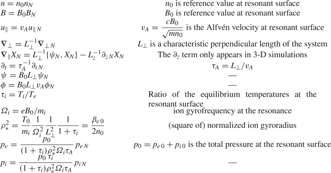
 is an index for the perpendicular geometrical coordinates. The normalization is detailed in table 1.
Normalization used for the equations of the model.

In slab geometry the vectorial Poisson bracket is defined as

In the above (2.11)–(2.16), the advection by the diamagnetic velocity cancels with the stress tensor through the gyroviscous cancellation, as detailed in Hinton & Horton (Reference Hinton and Horton1971), Hsu, Hazeltine & Morrison (Reference Hsu, Hazeltine and Morrison1986) and Smolyakov (Reference Smolyakov1998).
Comparison of these equations with those used in such models as GBS (Giacomin et al. Reference Giacomin, Ricci, Coroado, Fourestey, Galassi, Lanti, Mancini, Richart, Stenger and Varini2022), GDB (Zhu, Francisquez & Rogers Reference Zhu, Francisquez and Rogers2018) and GRILLIX (Zholobenko et al. Reference Zholobenko, Body, Manz, Stegmeir, Zhu, Griener, Conway, Coster and Jenko2021) shows that, up to vanishing electron mass, neglect of the effect of the thermal forces on the parallel drifts and the Boussinesq approximation, they are equivalent. Thus the energy conservation properties are analogous, with the appropriate corrections just mentioned.
An inspection of the equations (2.13) and (2.14) for the ion and electron pressures reveals that they are extremely similar in this reduced system, differing by the parallel velocity and the polarization term in the ion pressure. Indeed, it was observed that both pressures follow a very similar dynamics for the phenomenon and cases in question, so in (most of) the figures only the ion pressure will be shown, with the understanding that the electron pressure is following a similar dynamics.
In this paper, the model is used to describe the dynamics of magnetic islands generated by linearly unstable tearing modes. These allow us to recover the fundamental features of magnetic islands, meaning that what is described here should also exist for magnetic islands generated by other means, such as NTMs or turbulence-driven magnetic islands.
The model is implemented in the semi-spectral fluid code ‘AMON’. More details on the simulations will be given in § 4.
3. Heating of the island through parallel compression
The analysis of the fluid equations generating magnetic islands via unstable tearing modes in a 2-D symmetric system provides essential insight into the heating effect when one considers the parity of the fields (Muraglia et al. Reference Muraglia, Agullo, Benkadda, Yagi, Garbet and Sen2011; Ishizawa, Kishimoto & Nakamura Reference Ishizawa, Kishimoto and Nakamura2019). Focusing on a mono-helical, symmetric equilibrium magnetic field, the parity of the fields with respect to the resonant surface is going to be the following for the tearing mode (with ‘$+$ ’ indicating even and ‘$-$
 ’ indicating odd fields):

with phase relationships between the fields (taking the phase of the magnetic flux $\varphi _{\psi }$ for reference) given by

The relevant fields for the heating process are $p_{e/i}$ , $u_{\parallel }$
 and $\psi$
 , meaning, as will be detailed, that, in order to observe the heating in tearing modes, at least a four-field model ($\psi$
 , $\phi$
 , $p$
 and $u_{\parallel }$
 ) is required. Indeed, this phenomenon constitutes a channel to transfer energy first from the equilibrium current density gradient to the parallel velocity, through the presence of the tearing mode, and finally from the kinetic energy to the thermal energy, through the parallel compression, as will be now detailed.
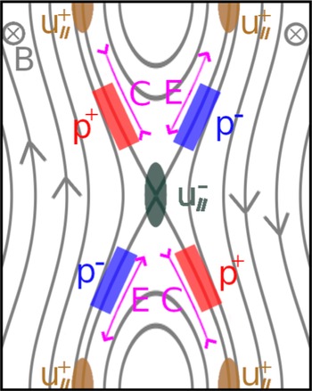
At the end of the linear growth phase of a tearing mode these four fields will have the configuration shown in figure 1, where the position of the extrema are schematically represented along the field lines, and the configuration of $\phi$ is analogous to that of $p$
 .
The coloured areas represent the spatial disposition of the extrema of the fields driving the heating process in the nonlinear phase of a linearly unstable tearing mode. The isocontours of $\psi$ are shown for reference. The compression (magenta ‘C’ in the figure) due to the parallel velocity structure corresponds to regions of positive pressure. The arrows on the grey lines indicate the direction of the magnetic field.

Compression is a mechanism by which kinetic energy can be converted to thermal energy, and vice versa for expansion. Considering only the configuration of $u_{\parallel }$ , the zones of expansion and compression are exactly symmetrical, both poloidally and radially, so that no net effect should result from the parallel dynamics when integrating over the whole volume. That is true if the pressure is considered as a constant parameter. Recalling, however, that the model considers the full pressure fields, including fluctuations, in the cubic terms in (2.13) and (2.14), it is not sufficient to consider the symmetry of the compression and expansion regions, but they must be taken together with the structure of the pressure fluctuations (see (2.1)). The latter have odd parity in tearing modes, and a phase difference in the poloidal direction of ${{\rm \pi} }/{2}$
 , as indicated in (3.2a,b). Hence, regions of compression correspond to regions of positive pressure fluctuations, and the opposite is true for expansion regions. This results in an imbalance between the two effects in favour of the positive pressure fluctuations (or, equivalently, the parallel compression regions) when integrated over the volume. The nonlinear dynamics then makes it so that these increasing pressures can enter the magnetic island through both diffusion and the quadrupolar flow, thus giving the localized heating that is being described.
It is then because the fields have the parities and relative phases indicated above that this phenomenon can be observed. In this paper the role played by the tearing mode instability is to maintain this configuration as stable throughout the whole simulation, thus allowing pressure accumulation. Much more generally, any mechanism generating a positive correlation between the pressure fluctuations and the parallel compression of the kind described is going to result in similar localized heating. What is meant by positive correlation is that $\int _{V} p \,\boldsymbol {\nabla }_{\parallel } u_{\parallel } \,{\rm d}V' > 0$ .
The heating is localized close to the separatrix until diffusion, advection or secondary instabilities allow the heat to spread further outside the island. The process has a positive feedback on itself, as $\partial _t p_{e/i} \propto p_{e/i}$ , and, in the absence of secondary instabilities, saturates if the pressure fluctuations are limited by the perpendicular diffusion and advection. The evolution of the averaged pressure profile is limited by the diffusivity, as it establishes a critical gradient for the system.
Note that all that has been said so far about the heating process applies analogously to the regions of parallel expansion, but the feedback loop means that the cooling effect in these regions is weaker, so that the heating ends up dominating.
Since the heating is localized at the separatrix, it is possible for gradients to develop near this layer, but the destabilization of secondary modes driven by pressure gradients was not observed, although it must be remembered that the curvature is suppressed in the present study. This might be due to the parallel diffusion inside the island allowing for partial flattening of the pressure inside the separatrix. The interaction of this phenomenon with turbulence will need to be further investigated.
4. Numerical simulations
4.1. Two-dimensional single-helicity simulations
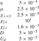
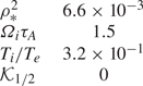
For nonlinear 2-D single-helicity (i.e. only one resonant magnetic surface in the system) simulations we consider only the magnetic equilibrium and no curvature for simplicity. The presence of heating does not depend on the dissipative (table 2) and equilibrium (table 3) parameters, as long as they are kept within ranges relevant for tokamak physics, but they can affect its rate and how localized it is around the resonance. In the present work, the only parameter far from a ‘realistic’ value is the resistivity $\eta$ , since the time required to reach saturation of magnetic islands in simulations for a physical $\eta \approx 10^{-8}$
 is excessively long, and the core physics are unaffected. The reference parameters correspond to a plasma with $\beta _0 = 2 p_0/B_0^2 = 0.02$
 at the resonance.
Dissipative parameters used for the reference simulation.

Physical parameters used for the reference simulation.

A grid with $512$ points on the $x$
 axis and $256$
 on the $y$
 axis was used for the simulations. The length of the $x$
 axis is $Lx = 4.0$
 and for the $y$
 axis $Ly = 2{\rm \pi}$
 . The fluctuations of the fields are initialized with random white noise at normalized amplitude $10^{-9}$
 .
The equilibrium magnetic profile is chosen to be the current density sheet Harris profile

with $A_H = 0.5$ being a multiplicative factor and the shear length $a_H = 0.5$
 determining the linear instability of the tearing mode with

Boundary conditions are periodic in the $y$ direction and impose that the perturbations are zero at either end on the $x$
 axis. Let us stress that the heating is not due to the presence or absence of any particular equilibrium gradient, except for $B_{eq}$
 , which is needed to drive the tearing mode. Indeed, the presence of heating was also verified in cylindrical geometry with an asymmetric equilibrium magnetic field for 2-D single-helicity simulations with similar results.
The attribution of the heating to the cubic terms is evidenced by the fact that removing the cubic terms in the simulations (e.g. $p_{e/i} \lbrace \psi, u_{\parallel } \rbrace$ becomes $p_r \lbrace \psi, u_{\parallel } \rbrace$
 , where $p_r$
 is the pressure at the resonance) removes the heating entirely.
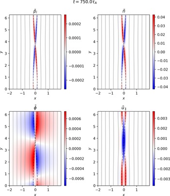
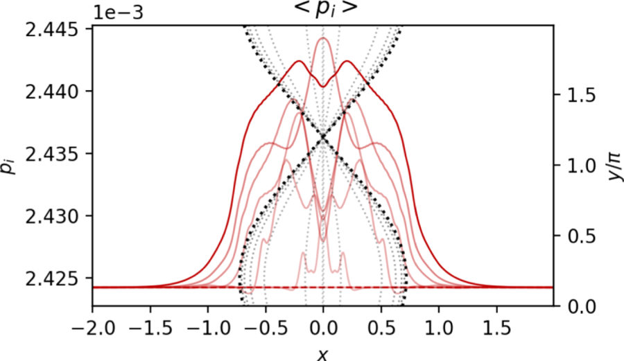
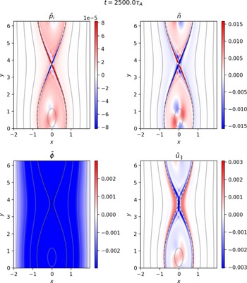
As shown in figure 2, the fields of interest for the heating process do indeed show tearing parity, and relative phases matching those in the heating scheme illustrated in figure 1. The evolution of the pressure profiles is shown in figure 3, where it is visible how the heating is centred on the island, with an alternation of peaking and hollowing at the resonant position. This is due to the formation of a quadrupole spinning around the $O$ -point, as visible in figure 4, late in the nonlinear phase. In the early nonlinear phase the heating is mostly on the separatrix, as that is where the compression takes place.
Poloidal maps of the fields relevant to the heating process for the ion pressure in the early nonlinear phase of the simulation. The parities and relative phase match those determined by the linearly unstable tearing.

Radial profiles of the pressure in the nonlinear phase of the 2-D simulation. Profiles go from transparent to opaque over time. The separatrix of the magnetic island at corresponding time is shown through the grey dotted lines as if placed on the $XY$ plane for reference.

Poloidal maps of the fields relevant to the heating process for the ion pressure in the saturation nonlinear phase of the simulation. The quadrupolar structures at the $O$ -point are spinning clockwise with $\nu _q \approx {2{\rm \pi} }/{245 \tau _A}$
 . The symmetry of the maximum and minimum values in the colour bars is enforced for $p_i$
 and $u_{\parallel }$
 for clarity: the actual data give $\vert \max (p_i) \vert > \vert \min (p_i) \vert$
 and vice versa for $u_{\parallel }$
 .

It is also to be remarked that the maximum value of pressure reached, even in cases where the equilibrium gradient of pressure was non-zero, is above the maximum value of the pressure in the equilibrium profile, meaning that the localized heating is not an effect of the transport of pressure, but is due to the additional thermal energy coming from the compression. As mentioned above, the maximum value of the pressure is ultimately limited by other mechanisms. Notably, a similar graph as in figure 6 for the density shows $\langle \partial _t n / n \rangle = 0$ for all simulations for the whole duration of the simulation, except for minor oscillation that do not cause a net ‘gain’ in density. This will be addressed in the discussion.
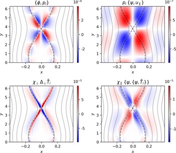
By calculating the terms that regulate the evolution of the heating, where the drive is given by $p_{e/i} \lbrace \psi, u_{\parallel } \rbrace$ , the advection by $\lbrace \phi, p_{e/i} \rbrace$
 and the dissipation by $\chi _{\parallel } \lbrace \psi, \lbrace \psi, \tilde {T}_{e/i} \rbrace \rbrace$
 and $\chi _{\perp } \varDelta _{\perp } \tilde {T}_{e/i}$
 (see figure 5), one can verify that they do indeed all act around the $X$
 -point in the nonlinear phase, where the pressure fluctuations can enter the island. The advection by the quadrupolar flows balances, although not entirely, the parallel compression to try and maintain incompressibility, thus transporting the pressure inside the island. The remaining part of the compression term which is not advected is dissipated by the parallel and perpendicular diffusion. The relative magnitude of all these terms changes significantly over the course of the simulation, mostly due to the pressure increasing until the transport balances its growth and the other fields saturating due to the ‘regular’ saturation of the magnetic island.
Poloidal maps of the terms involved in the heating for 2-D simulations. Note that their relative magnitude changes significantly throughout the simulations. A symmetric range of values was enforced on all maps to ensure that the colour white would correspond to the value $0$ , thus the asymmetry of positive and negative values is not clearly visible, especially in the top right panel.

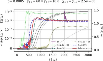
As shown in figure 6, the intensity of the heating has a dependence on $\eta$ , but not at all on $\beta$
 , the latter only acting to anticipate or delay the transition to the nonlinear phase. Fitting the results of the available simulations shows that, in the saturated nonlinear phase, the heating rate scales as $\eta ^{1.7}$
 . While this point has not yet been entirely clarified, it is observed that the amplitude of the fluctuations for all fields except $\psi$
 and $\phi$
 at saturation is directly affected by the resistivity, and so is the width of the eigenmodes around the separatrix. The combination of these two effects is probably what determines the dependence on $\eta$
 . The simulations with different $\beta$
 in figure 6 indicate that the width of the modes, which is most affected by the dissipations, is the dominant parameter to determine the heating, as otherwise the different magnitude of the pressure fluctuations would show its effect. Furthermore, as is visible in figure 6, the heating rate saturates before the island has properly started to grow, suggesting once more that the heating rate is a function of the resistive layer width, which is established in the linear phase, rather than the island size.
Dependence of the heating rate on the resistivity. In the run labelled $\Delta \eta$ the resistivity is $\eta = 2.5\times 10^{-03}$
 up to $t=2000\tau _A$
 , and it is then changed to the reference value $\eta = 5.0\times 10^{-04}$
 , thus showing a direct dependence of the heating on the resistivity. The simulation with lowest $\eta = 1.0\times 10^{-04}$
 did not reach saturation of the island in the time frame shown, as the heating saturates much earlier. In grey scale are the island sizes matching the simulations with the same line style.

It is also possible that the scaling obtained is only valid for the large $\eta$ regime considered here, and that some other dissipative process dominates once the values of $\eta$
 approach a more physically relevant range $\eta \approx 10^{-8}$
 . The amplitude and the width of the fluctuations would then no longer scale with $\eta$
 as indicated, but the heating process should be present nonetheless.
4.2. Three-dimensional multi-helicity simulations
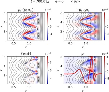
Examination of the effect in nonlinear 3-D multi-helicity simulations has shown that it is still present and driven by the same process (see figure 7, top left, top right and bottom right panels), but the behaviour of the heating, especially with respect to its localization, its intensity and its dynamics, is much more dependent on the specifics of the system than in the 2-D case. For brevity, the details about the behaviour of this phenomenon in 3-D simulations are left for another time, and we give here only a quick overview and confirmation of its existence also in 3-D cylindrical simulations.
Poloidal maps showing the terms relevant to the heating in 3-D multi-helicity simulations at a specified toroidal position $z = 0$ , in the early nonlinear phase. In the bottom right panel in red is overlayed the averaged radial profile of $p_i$
 to show the position where the heating is localized. The dashed black lines show the position of the resonance and of the separatrix for the $q=2$
 modes at the same time point. The isocontours of the mode $(2,1)$
 of the poloidal magnetic flux are shown for reference.

The simulation parameters in 3-D multi-helicity are analogous to those in the 2-D single-helicity case, as are the boundary conditions, with the addition of periodicity on the $z$ axis. Even in this case we were not able to find parameters where the heating did not appear. A grid with $256$
 points on the $x$
 axis, $64$
 on the $y$
 axis and $32$
 on the $z$
 axis was used for the simulations shown. The $y$
 and $z$
 axes are de-aliased by only retaining modes up to $2/3$
 of the maximum mode number.
The profile of the safety factor $q = (B_z r) / (B_{\theta } R_0)$ is chosen to be of the form

with $q_0 = 1.7$ , $q_1 = 4.5$
 , $L_{x_0} = 0.3$
 being the leftmost boundary of the simulation box and $L_x = 1.2$
 being the width along the $x$
 -axis of the simulation box. This positions the resonance for $q=2$
 at $x\approx 1.13$
 (the vertical dashed black line in figures 7 and 8). Other geometrical parameters are the size along $y$
 and $z$
 of the simulation box $L_y = 2{\rm \pi}$
 and $L_z = 3{\rm \pi}$
 . This set-up ensures that only the mode $(m,n) = (2,1)$
 is linearly unstable.
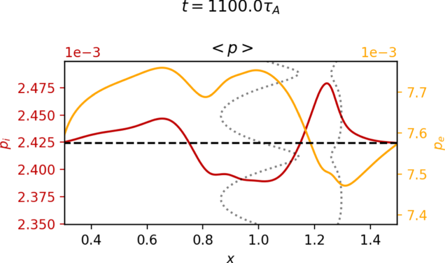
Radial profiles of the electron (orange) and ion (dark red) pressure in the nonlinear phase of the 3-D simulation. The dashed black line is the initial value for both axes $p_e$ and $p_i$
 . The separatrix of the magnetic island is shown dotted in grey as if placed on the $XY$
 plane for reference. All elements are shown at $z=0$
 .

The additional 3-D terms represent the fluctuations in the ‘toroidal’ ($z$ in this article) direction, and are introduced in the system through the expression of the parallel gradient

This addition is particularly important as the nonlinear couplings in the Poisson bracket and in the cubic terms will then also couple toroidal fluctuations, making the dynamics more complex. Still, it can be seen in figure 7 that the Poisson bracket and the $\partial _z$ derivative act the same way, although with different magnitudes, thus allowing the heating to appear through the same process described above. This might be in large part due to the presence of a single dominant $(2,1)$
 mode and the low level of fluctuations in the simulation, so more extensive study of the phenomenon in three dimensions needs to be carried out, but it is consistent with the picture obtained from the 2-D simulations.
As is known from the literature (Poye et al. Reference Poye, Agullo, Benkadda, Garbet and Smolyakov2011; Smolyakov et al. Reference Smolyakov, Poye, Agullo, Benkadda and Garbet2013), in cylindrical geometry with an asymmetric equilibrium magnetic field the tearing mode grows mostly on the inner side of the resonance. This then means that the $\boldsymbol {E} \times \boldsymbol {B}$ flows transporting the magnetic field lines are only present on one side, resulting in a net shift of the $O$
 -point in one direction and of the $X$
 -point in the opposite. This shift is visible in the isocontours of $\psi _{(2,1)}$
 in figure 7. Also visible in figure 7, because the tearing mode is mainly growing on one side, $p_i$
 does not have two regions of opposite sign across the resonance, but rather across the separatrix and, due to the radial shift of the island, it is non-null on the resonance. Furthermore, the radial profile of $p_i$
 , shown as the continuous line in the bottom right panel of figure 7, is only increasing on one side of the resonance, which is the opposite of the side where $p_e$
 is growing, as visible in figure 8. Regardless of these additional elements, the phase differences in the fields are the same as those found in the 2-D case, and the other terms, like $\lbrace \phi, p_i \rbrace$
 , play the same role. In other words, the heating mechanism is present in 3-D simulations despite the fields not having the same radial structure as in the 2-D case and the presence of asymmetric geometry and of the 3-D terms.
As visible in figure 8, both pressures are much less localized on the island than in 2-D single-helicity simulations, and radially show alternating positive and negative regions, that overall weaken, but do not suppress, the heating. In figure 8 both pressures are included to show that while in the 2-D case electrons and ions have the same dynamics, the 3-D case introduces more complexity. Late in the nonlinear phase both pressures run into the limits imposed by the boundary box due to the heating spreading much more efficiently outside of the separatrix. The specifics of the profile shapes vary depending on the simulation parameters, but the heating shows up consistently.
5. Discussion
A heating process in magnetic islands generated by linearly unstable tearing modes was described, and its presence verified in both 2-D single-helicity and 3-D multi-helicity simulations performed with a six-field electromagnetic fluid model. The heating is shown to be due to the presence of cubic terms in the equations for the pressure evolution that involve the product of the compression of the parallel velocity and the pressure fluctuations in proximity of the separatrix.
Let us emphasize that a model with the same fields but that does not retain the full cubic terms would miss the heating mechanism described in this paper. On the other hand, using a lower number of fields could simplify the analysis a bit, but at least four fields ($\psi$ , $\phi$
 , $p$
 and $u_{\parallel }$
 ) would be needed. Moreover, restricting the model to four fields would no longer allow us to study the interaction between the magnetic island (eventually NTMs) and toroidal ITG turbulence.
It has been shown that, in order for the heating to take place, the parity and relative phase of the fields must allow for the positive match between parallel compression and pressure fluctuations, which in the present case was obtained by having a current-driven linearly unstable tearing mode. The quadrupolar flow determined by the tearing mode further contributes to advect the fluctuations inside the island (see figure 5). This list of features is expected to be present not only for tearing modes, but more generally whenever a magnetic island is present, including the case where a locked magnetic island is externally induced. It follows that the finding of heating inside an induced magnetic island, in Choi et al. (Reference Choi, Bardōczi, Kwon, Hahm, Park, Kim, Woo, Park, Yun and Yoon2021), might be linked to the heating mechanism described in this paper. The absence of background turbulence in the simulations shown did not allow us to observe the propagation of the fluctuations to the $X$ -point as described in the experiment (Choi et al. Reference Choi, Bardōczi, Kwon, Hahm, Park, Kim, Woo, Park, Yun and Yoon2021), but it was observed that the pressure fluctuations causing the heating enter the island at the $X$
 -point through the quadrupolar flows (see figure 5) and tend to accumulate in the centre as a spinning quadrupole. This motivates further investigations about the interaction of magnetic islands and turbulence, that will be carried out in future work to check whether the same turbulence propagation dynamics as observed experimentally can be recreated in simulations. In particular, in the experiments the heating is shown to be much more focused in the centre of the island than on the separatrix, as in the present case, and the expulsion of the heat observed in experiments was not replicated in our simulations to the degree where the hot-spot disappears completely. Whether these effects might be due to the presence of turbulence and/or to different processes remains to be studied and clarified.
The heating effect can be expected to be present both in the presence of background turbulence and for turbulence-driven magnetic island, as it has been shown (Hornsby et al. Reference Hornsby, Migliano, Buchholz, Zarzoso, Casson, Poli and Peeters2015) that turbulence does not alter the mode structure, but such a prediction needs to be verified. Indeed, once the fluctuations of $p$ and $u_{\parallel }$
 are no longer driven by the tearing mode but by turbulence, it can be expected that the properties of the process, especially its magnitude, will change.
Since this is a phenomenon that has a direct (and dominant in the present study) impact on the pressure profiles, an open question is why it is not commonly observed in experimental measurements. There are clues about this in the scaling with $\eta$ mentioned in § 4.1, and the magnitude of the effect itself, nevertheless there should be hints of this effect in the regime of large islands in which tokamaks operate when a magnetic island is present for any significant duration of time (see figure 9).
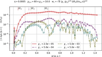
Dependence of the heating on the critical width (see (5.1)) of the island. To obtain different critical island widths the ratio $\chi _{\perp }/\chi _{\parallel }$ is varied. Empty circles (diamonds) represent positive (negative) average heating rate for a given island width. The more the plasma operates in the large island regime the more the heating is prominent. The critical island widths are indicated at the top of the graph with line styles matching those of the simulations in the legend.

It is also the case that the heating is stronger if the plasma operates in the large island regime. In figure 9 a scan of the heating effect is performed for varying critical widths, above which the equilibrium pressure profile is expected to be flattened, of the island, as defined in Fitzpatrick (Reference Fitzpatrick1995)

where $R_0$ is the major radius of the torus, $n_{{\rm tor}}$
 the mode of the toroidal mode and $s = \partial _r B_{{\rm eq}} / B_{{\rm eq}}$
 the magnetic shear.
More precisely, in figure 9, four simulations with different perpendicular diffusivities $\chi _{\perp }$ are performed, and each point represents the average heating rate for the given island size. The rightmost point corresponds to the saturation of the dynamics, thus the saturated island size. The result is that the larger the ratio between the saturated island size $w$
 and the critical width $w_c$
 , the more the heating $\langle \partial _t p_s / p_s \rangle$
 is active throughout the simulation, while it tends to disappear in the opposite case. However, simulations (not shown) run with different ‘toroidal’ lengths of the simulation boxes and $\chi _{\parallel }$
 , and thus different $w_c$
 , have approximately identical behaviour with respect to the heating, thus indicating that the behaviour of the heating is mostly due to the perpendicular diffusivity itself, rather than to the critical island width, as is the case for pressure flattening. Indeed, if the perpendicular dissipation is large enough to prevent the accumulation of the pressure on the separatrix, the heating hardly appears at all and there is a phase of decrease in pressure. In this case the electrons show a slightly different behaviour where, even for large $\chi _{\perp \, e}$
 the heating is present in the initial phase of the island growth, and then drops to $0$
 much later. This is further indication that in experiments where the ratio $\chi _{\perp } / \chi _{\parallel }$
 is smaller than considered here, this effect should be non-negligible, and should be at play through the whole plasma discharge.
It is important to address why no average accumulation is observed for the density even though its parity and phase match those of the pressure. A ‘bump’ in the density inside the separatrix is indeed visible, not unlike in figure 3, but it is matched by regions of negative density fluctuations outside the separatrix, that bring the average over the simulation box to $0$ . This is characteristic of a transport phenomenon, whereby no net increase is obtained but the field is transported inside the separatrix, rather than having exchange of energy from one field to another. This is of course reasonable as the only way for the density to increase globally is through fuelling, while the pressure can be increased through compression. In figure 4 the same fields shown in figure 2 are shown late in the saturation phase. Notice that, while inside the separatrix $p_i$
 and $n$
 are very similar, with a spinning ($\nu _q \approx {2{\rm \pi} }/{245 \tau _A}$
 ) quadrupolar structure at the $O$
 -point, outside the separatrix the pressure has a positive ‘band’, while for the density it is negative, contributing to the $0$
 average. Also, overall, the positive fluctuations have higher absolute value than the negative ones for $p_i$
 , while for $n$
 they are symmetric, even in the quadrupole in the centre, so for the pressure there is a net increase, that cannot be justified, as was already mentioned, by transport phenomena. In sum this is properly heating in the sense of a temperature increase.
When discussing the effect of this phenomenon on realistic scenarios, it is also important to point out that the pressure generated by the heating mechanism has quadrupolar structure (see figure 5 top right panel), and will thus enhance the reconnection rate in the plasma, which has been checked in simulations, giving a $10\,\%$ increase in the reconnection rate $\partial _t \vert \langle \psi _{m=1} \rangle \vert$
 during the growth phase of the island for large resistivity ($\eta = 10^{-3}$
 ).
In future works, it will be very interesting to consider the effect on the resistivity of the localized heating. This is going to be relevant for both tearing modes and NTMs (Callen & Shaing Reference Callen and Shaing1985; Carrera et al. Reference Carrera, Hazeltine and Kotschenreuther1986) (as are the direct effects on the pressure profiles) since considering a very basic Spitzer $\sim T^{-3/2}$ scaling law, this heating would locally reduce the resistivity, thus affecting the current and finally the dynamics in the island.
Results from simulations show that the term responsible for the cumulative heating effect ranges from roughly one tenth of the $\boldsymbol {E} \times \boldsymbol {B}$ advection term at the beginning of the nonlinear phase to the same magnitude at saturation. This further proves that the phenomenon should not be ignored as a curiosity. Note that other phenomena (Agullo et al. Reference Agullo, Muraglia, Benkadda, Poyé, Dubuit and Garbet2017a; Dudkovskaia et al. Reference Dudkovskaia, Connor, Dickinson, Hill, Imada, Leigh and Wilson2021) have already been found to limit the flattening of the pressure profile expected (Fitzpatrick Reference Fitzpatrick1995) and observed (Snape et al. Reference Snape, Gibson, O'gorman, Barratt, Imada, Wilson, Tallents and Chapman2012) to happen in a magnetic island. Unlike those studies, however, the presently described phenomenon is present at all times in the evolution of a magnetic island, provided that the fields retain their parities and relative phases and that no other effect intervenes to disrupt the structure of the fields.
In conclusion, this analysis suggests that the dynamics of magnetic islands should be investigated more in depth at a fundamental, rather than heuristic, level, in particular when it comes to the dynamics of the parallel flow. The heating also relies on the presence of magnetic fluctuations in the system, thus being of relevance for high-$\beta$ regimes (Sauter et al. Reference Sauter, La Haye, Chang, Gates, Kamada, Zohm, Bondeson, Boucher, Callen and Chu1997), and its scaling with the diffusivity makes it even more relevant for the low collisionality regimes in large tokamaks.
Acknowledgements
The authors would like to thank M. Muraglia and P. Maget for fruitful discussions. The project leading to this publication has received funding from the Excellence Initiative of Aix-Marseille University – A*Midex, a French ‘Investissements d'Avenir’ program AMX-19-IET-013. The simulations in this article were run thanks to the support of EUROfusion and MARCONI-Fusion. This work has been carried out within the framework of the EUROfusion Consortium, funded by the European Union via the Euratom Research and Training Programme (Grant Agreement No 101052200 – EUROfusion). Views and opinions expressed are, however, those of the author(s) only and do not necessarily reflect those of the European Union or the European Commission. Neither the European Union nor the European Commission can be held responsible for them. Centre de Calcul Intensif d'Aix-Marseille is acknowledged for granting access to its high performance computing resources.
Editor Francesco Califano thanks the referees for their advice in evaluating this article.
Declaration of interests
The authors report no conflict of interest.
Appendix A. Derivation of the equation for the perpendicular motion
There are some additional terms in the equation for the perpendicular momentum (2.12) used in this work with respect to more ‘conventional’ reduced fluid models, these being the second and third terms on the right-hand side of (2.12). These terms come about from the inclusion of finite Larmor radius effects in the model through the polarization drift, so that the role of the gyro-motion of the ions may be taken into account in the fluid model. The magnitude of these effects scales as the ion Larmor radius $\rho _i = \sqrt {T_i/m_i} \cdot \varOmega ^{-1}_i$ and they are expected to play a significant role as the $\beta$
 of the plasma increases, or, more generally, when one wants to look at phenomena happening at the ion scale. Since the original goal for the development of the model was studying ion-scale turbulence and instabilities (namely ITG-driven instabilities), the inclusion of Finite Larmor Radius (FLR) effects was needed to be able to carry out the analysis. The existence of the heating mechanism described in this paper is not dependent on these terms. Here, some detail on their derivation and physical significance is provided, and further discussion can be found in papers that employ similar models (Scott Reference Scott2001, Reference Scott2021; Zholobenko et al. Reference Zholobenko, Body, Manz, Stegmeir, Zhu, Griener, Conway, Coster and Jenko2021; Giacomin et al. Reference Giacomin, Ricci, Coroado, Fourestey, Galassi, Lanti, Mancini, Richart, Stenger and Varini2022).
Since we are using the Boussinesq approximation, and neglecting advection by $\boldsymbol {u}_I$ , the left-hand side of (2.7) gives

The compression of $\boldsymbol {u}_I$ should be retained since the drift is non-ambipolar, and thus, in order to maintain quasi-neutrality, its role is significant. On the other hand, advection by $\boldsymbol {u}_I$
 would act on the gradients of $n_{eq}$
 (and $p_{i \, eq}$
 in the ion pressure equation) to higher order than the other drifts, and add to the nonlinearities also at higher order, so that it being neglected is not expected to have any significant impact on the dynamics.
One can re-write (A1) (neglecting constants and only keeping the $E \times B$ advection for clarity) as

Using vector identities, the second term on the right-hand side of (A2) can be re-written as

And further, ignoring the known term $\{ \phi, \mathcal {W} \}$

This term is not properly a Poisson bracket as it involves two vectors, but for convenience of notation we write it as above. It is a term that describes FLR components in the stress tensor, these being due to the exchange of momentum between the diamagnetic and the $E \times B$ drifts for ion-scale motions, and is a further correction to the already known $\{ \phi, \mathcal {W} \}$
 stress tensor term. Given the high-order derivatives it involves, this term plays a significant role only in the nonlinear evolution of the system. Explicitly, in slab geometry it is the following contraction:

Since the Poisson bracket of a field with itself is $0$ , from the $W$
 in (A5) only the pressure component gives a non-zero contribution, recovering the second term on the right-hand side of (2.12).
Doing the same derivation for the parallel drift

This term represents the parallel advection of vorticity fluctuations along the field lines, and is kept in order to be consistent with the choice of not applying flute ordering.