1 Introduction
1.1 Model and relations with existing models
We consider an inhomogeneous SIS epidemic model, where individuals are either susceptible or infected. The homogeneous model was introduced by Kermack and McKendrick [Reference Kermack and McKendrick28], we refer to the monograph of Brauer, Castillo-Chavez, and Feng [Reference Brauer, Castillo-Chavez and Feng9] for an analysis of this homogeneous SIS model and some of its variants. Let us recast the model from [Reference Kermack and McKendrick28] in the constant population case: let
 and
 $S(t)$
denote, respectively, the number of the infected and susceptible individuals at time
 $t \geq 0$
, in a population of constant size
 $N=S(t)+I(t)> 0$
. The evolution of the number of infected is given by
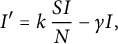 $$ \begin{align} I' = k \,\frac{SI}{N} - \gamma I, \end{align} $$
where
 $k \geq 0$
is the infection rate and
 $\gamma> 0$
the recovery rate.
The assumption of homogeneity of the population is not always satisfied in practice, see, for example: Trauer et al. [Reference Trauer, Dodd, Gomes, Gomez, Houben, McBryde, Melsew, Menzies, Arinaminpathy, Shrestha and Dowdy54] for a review on tuberculosis, [Reference Popkin, Du, Green, Beck, Algaith, Herbst, Alsukait, Alluhidan, Alazemi and Shekar43] on the impact of health condition, [Reference Britton, Nordvik and Liljeros11] on the number of sexual partners in a sexually transmissible infection, or the review [Reference VanderWaal and Ezenwa55] for more possible sources of heterogeneity. The inhomogeneous SIS model from Lajmanovich and Yorke [Reference Lajmanovich and Yorke32] generalizes the Kermack–McKendrick model to a population divided in n sub-groups; the same equation appears also when studying network of communities linked by dispersal (see Mouquet and Loreau [Reference Mouquet and Loreau40] and more generally [Reference Cantrell, Cosner, Lou and Schreiber12]. Later, Thieme [Reference Thieme53] and Delmas, Dronnier, and Zitt [Reference Delmas, Dronnier and Zitt17] introduced a variant allowing an infinite number (possibly uncountable) of sub-groups or features.
We follow the model given by [Reference Delmas, Dronnier and Zitt17] where the transmission operator can be non-irreducible, see the discussion in Section 1.2 below and allowing furthermore a more general incidence rate (see Section 1.5). The heterogeneity of the population is described as follows:
 $(\Omega , \mathcal {G}, \mu )$
is a measured space with a nonzero finite measure
 $\mu $
: an element
 $x\in \Omega $
corresponds to a particular feature (or trait) of individuals. We assume that individuals with the same feature behave in the same way with respect to the epidemic, and that features stay constant during the whole infection process. We also assume that for a given feature
 $x \in \Omega $
, the size of the population
 $\mu (\mathrm {d} x)$
of feature x remains constant over time.
Let
 $u(t,x)$
denote the proportion of individuals with feature
 $x\in \Omega $
that are infected at time
 $t\geq 0$
among the population of individuals with feature x. Let
 $\Delta $
be the set of measurable functions defined on
 $\Omega $
taking values in
 $[0, 1]$
. The heterogeneous SIS dynamics is given, for an initial condition
 $h \in \Delta $
, by the evolution equation on the Banach space
 $L^\infty $
of measurable bounded real-valued functions defined on
 $\Omega $
by
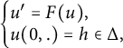 $$ \begin{align} \left\{\begin{array}{@{}l} u' = F(u), \\ u(0,.) = h\in \Delta, \end{array}\right. \end{align} $$
with
 $$ \begin{align} F(u)= \varphi(u)\, Tu - \gamma u, \end{align} $$
where F depends on: a bounded positive linear transmission operator T on
 $L^\infty $
, a bounded real-valued positive recovery rate function
 $\gamma $
defined on
 $\Omega $
, and a real-valued function
 $\varphi $
defined on
 ${\mathbb {R}}$
encoding the non-bilinearity of the incidence rate. The hypotheses on the parameter
 $(T, \gamma , \varphi )$
are given in Assumptions 1 and 2 (see Section 1.3). Let us stress that the usual law of mass action
 $\varphi = 1-\operatorname {\mathrm {Id}}$
, with
 $\operatorname {\mathrm {Id}} $
the identity map on
 ${\mathbb {R}}$
, satisfies the corresponding hypothesis from Assumption 2 summarized in Condition (1.14).
Remark 1.1 (The kernel model from [Reference Delmas, Dronnier and Zitt17])
Let
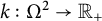 $k : \Omega ^2 \rightarrow {\mathbb {R}}_+$
be a kernel, that is, a nonnegative measurable function. The associated kernel operator
 $T_k$
is defined as follows. For
 $h\in L^\infty $
and
 $x \in \Omega $
, such that
 $k(x,\cdot ) h(\cdot )$
is integrable, we define
 $$\begin{align*}T_k (h) (x) = \int_\Omega k(x,y) h(x) \, \mu( \mathrm{d} y). \end{align*}$$
The quantity
 $k(x,y)$
represents the transmission rate from individuals with feature
 $y\in \Omega $
to those with feature
 $x\in \Omega $
. The heterogeneous SIS model from [Reference Delmas, Dronnier and Zitt17] is then given by (1.2) and (1.3) with
 $T=T_k$
(under some integral hypothesis on the kernel) and the usual law of mass action
 $\varphi = 1-\operatorname {\mathrm {Id}}$
. This, in particular, encompasses the Lajmanovich and Yorke model.
In epidemiology, equilibria are constant solutions of (1.2), that is, functions
 $g\in \Delta $
such that
 $$ \begin{align} F(g) = 0. \end{align} $$
They play a significant role in the long-time behavior of the dynamics of an outbreak (see Theorem 3 below). Obviously, the disease-free equilibrium (DFE)
 $g = 0$
is an equilibrium. Any other equilibrium is called endemic equilibrium (EE). The basic reproduction number denoted
 $R_0$
is defined by Heesterbeek and Dietz [Reference Heesterbeek and Dietz27] as “the expected number of secondary cases produced by a typical infected individual during its entire infectious period, in a population consisting of susceptibles only”. Following [Reference Delmas, Dronnier and Zitt17] (see also the method of the next-generation operator in Diekmann, Heesterbeek, and Metz [Reference Diekmann, Heesterbeek and Metz20]), the basic reproduction number
 $R_0$
for the SIS model (1.2) with the usual incidence rate associated with
 $\varphi =1- \operatorname {\mathrm {Id}}$
is defined as the spectral radius of the operator
 $T M_{1/\gamma }$
, where the operator
 $M_{1/\gamma }$
is the multiplication by
 $1/\gamma $
. There usually is a threshold behavior for the existence of EE according to the value of
 $R_0$
: for
 $R_0 \leq 1$
, only the DFE exists as an equilibrium, and for
 $R_0> 1$
, there exists an EE. This is not universal: for example, models with imperfect vaccines or exogenous re-infections might lead to backward bifurcation and produce multiple EE even in the regime
 $R_0 < 1$
(see [Reference Gumel24] and, more specifically, [Reference Brauer8] for an SIS model). Nevertheless, we check that threshold behavior holds for the SIS model (1.2) (see Theorem 2 below). A discussion of the uniqueness of EE is given in Section 1.2.
1.2 A taste of the main results in the finite setting
1.2.1 Framework and examples
Except in the trivial case where the population may be split in sub-populations that do not interact at all, the existence of multiple equilibria is fundamentally linked to asymmetry in the transmission dynamics. In this section, we first explain this phenomenon, and a related crucial decomposition of the space, in the simple case where
 $\Omega $
is finite, to give a taste of the general results stated below.
We consider a finite set
 $\Omega $
, let
 $\mathcal {G}$
be the set of subsets of
 $\Omega $
, and
 $\mu $
a finite measure with support
 $\Omega $
. The transmission operator T is identified with a matrix
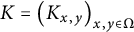 $K=\left ( K_{x,y} \right )_{x,y\in \Omega }$
where
 $K_{x,y}\geq 0$
is the infection rate from individuals with feature y to those with feature x; in particular, it takes into account the relative size of the sub-populations. When
 $\Omega $
is a singleton and
 $\varphi = 1-\operatorname {\mathrm {Id}}$
, we recover Equation (1.1) (with
 $u = I/N$
and
 $K=k$
). When
 $\Omega $
is finite, we recover the Lajmanovich and Yorke [Reference Lajmanovich and Yorke32] model, and the same framework can be used to describe households models [Reference Ball6] and multi-host and vector-borne diseases [Reference McCormack and Allen39].
In this finite case, the study of the non-uniqueness for equilibria relies on the properties of the oriented transmission graph
 $G_K=(\Omega , E_K)$
with the set of edges
 $E_K=\{(y,x)\in \Omega ^2\, \colon \, K_{x,y}>0\}$
given by the support of the transmission matrix K. An edge from y to x models the possibility of infection from the sub-population with feature y to the sub-population with feature x; in particular, the graph may have self-loops. For transmission graph models, see, for example, [Reference Arino5, Reference Guo, Li and Shuai25].
Strongly connected components of
 $G_K$
will be called atoms – the notion will be generalized in the infinite case. An atom is nonzero unless it is a singleton with no self loop. Notice the transmission matrix/operator is irreducible if and only if the graph
 $G_K$
is strongly connected (that is,
 $\Omega $
is an atom), and is said monatomic if there is a unique nonzero atom. For further result on monatomic operators in the general case, see [Reference Delmas, Lefki and Zitt19] and references therein; we refer also to Corollary 4.11 for a characterization of monatomic transmission matrix using the number of EE.
In many examples, the transmission graph
 $G_K$
is symmetric (even though the transmission K might not be symmetric). In this case, all (strongly) connected components behave independently and one can study each connected components separately. Cases where
 $G_K$
is not strongly connected occur less frequently in the literature; it has been mentioned, for example, in a multi-type SIR model by [Reference Knipl and Röst29, Reference Magal, Seydi and Webb36]. Let us mention two examples of nonsymmetric transmission graphs.
-
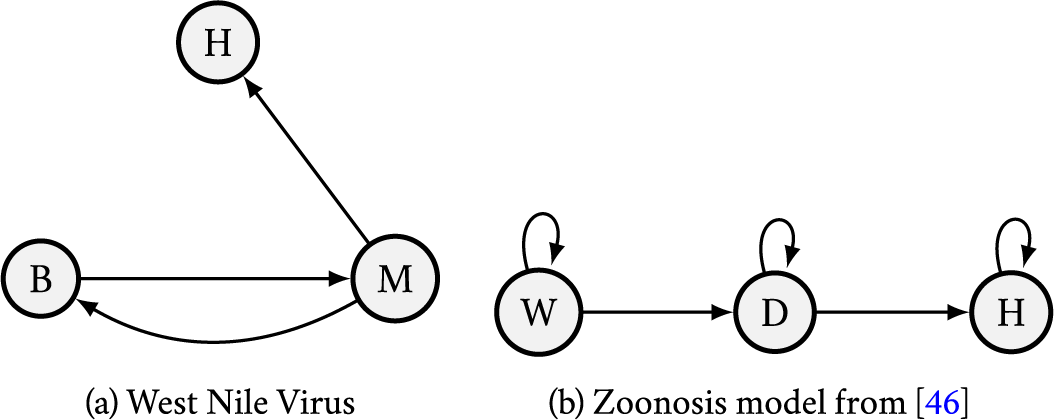
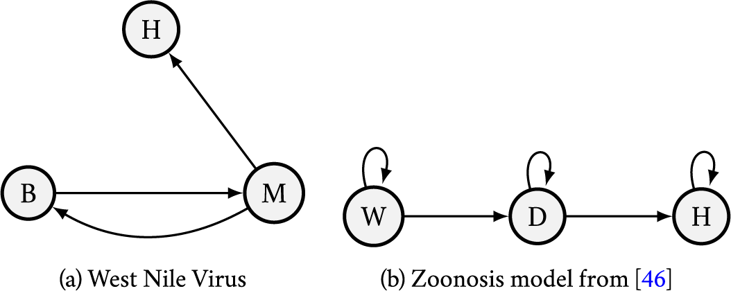
(1) The West Nile Virus, presented in [Reference Bowman, Gumel, Van den Driessche, Wu and Zhu7], infects three species, birds (B), humans (H), and mosquitoes (M). It is a vector-borne disease where birds and mosquitoes serve as vectors for a transmission to humans. In this model, mosquitoes infects birds and humans while biting them and mosquitoes get infected by birds while biting them, and we assume there is no infection from humans to mosquitoes, nor between birds and humans. The graph
 $G_K$
given in Figure 1a has only one nonzero atom
$\{B,M\}$
and a zero atom
$\{H\}$
. In particular, K is monatomic.Figure 1:
Some examples of transmission graphs
$G_K$
. -
(2) In the zoonosis model from [Reference Royce and Fu46], a pathogen exists in wild animals (W) is transmitted to domestic animals (D) that transmit themselves the pathogen to humans (H). The graph
$G_K$
given in Figure 1b has three nonzero atoms:
$\{W\}, \{D\},$
and
$\{H\}$
.




In such cases where
 $G_K$
is not symmetric, the picture is richer: many endemic equilibria may exist, they may be entirely characterized by the atoms contained in their support, and their basins of attraction may be described explicitly.
Let us give a few additional definitions to state these results more precisely, before giving the general statements below in Theorems 2 and 3. Define the future of a set
 $A\subset \Omega $
as the set
 $\mathcal {F}(A)$
of all the vertices in
 $G_K$
reachable from A by a (possibly empty) path using edges in
 $E_K$
. For two atoms A and B of
 $G_K$
, we write
 $B \preccurlyeq A$
if
 $ B\subset \mathcal {F}(A)$
; the relation
 $\preccurlyeq $
is a partial order. An antichain of atoms is a set of atoms which are pairwise unordered. The future of an antichain is the future of the union of its elements.
In the West Nile Virus model i, the antichains of nonzero atoms are
 $\emptyset $
and
 $\{B,M\}$
; in the zoonosis model ii, the antichains of nonzero atoms are:
 $\emptyset $
,
 $\{H\}$
,
 $\{D\}$
, and
 $\{W\}$
.
Finally, an atom is supercritical if the basic reproduction of the SIS-model restricted to the atom is larger than 1; in particular, a supercritical atom is nonzero and an atom A is trivially supercritical if
 $K_{x,x}/\gamma (x)>1$
for all
 $x\in A$
, where
 $\gamma $
is the recovery rate function, and the function
 $\varphi $
satisfies the regularity Condition (1.14) below.
1.2.2 Main results in the finite case
Our first main result, Theorem 2, states (in the general possibly infinite setting) that each equilibrium is characterized by a (different) antichain of supercritical atoms, and the DFE is associated with the antichain
 $\emptyset $
. For example, assuming for simplicity that all nonzero atoms are supercritical, we deduce that in the West Nile Virus model i there is only one EE and that in the zoonosis model ii there are three EE.
Let us mention that a similar result on the existence of multiple EE is obtained in Waters et al. [Reference Waters, Hamilton, Sidhu, Sidhu and Dunbar56] for a waterborne parasites that infect both humans and animals, such as Giardia infection in rural Australia. In this model, the animals and the humans can be seen as nonzero atoms for the transmission, and the water as an environmental reservoirs. This model does not fit exactly the metapopulation SIS model (1.2) and (1.3), nor the model with external disease reservoir presented in Section 1.4 because the reservoir is between the animal population and the human population.
Theorem 2 also states that the support of an equilibrium is given by the future of its corresponding antichain of supercritical atoms. Furthermore, Corollary 4.2 asserts that for two equilibria g and
 $g'$
, we have
 $g\leq g'$
if and only if
 $\operatorname {\mathrm {supp}}(g)\subset \operatorname {\mathrm {supp}}(g')$
. This, in particular, allows to recover the existence of a maximal equilibrium
 $g^*$
, in the sense that if g is an other equilibrium, then
 $g\leq g^*$
.
For example, assuming again for simplicity that all nonzero atoms are supercritical, we deduce that in the zoonosis model ii, denoting by
 $g_x$
the equilibrium characterized by the antichain
 $\{x\}$
, we have
 $$\begin{align*}\operatorname{\mathrm{supp}} (g_H) &=\{H\}\subset \operatorname{\mathrm{supp}} (g_D)=\{D, H\}\subset \operatorname{\mathrm{supp}}(g_W) \\ &=\{W,D,H\} \quad\text{and}\quad 0\neq g_H\lneqq g_D\lneqq g_W=g^*. \end{align*}$$
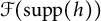
Our second main result is a full characterization of basins of attraction of the various equilibria: we show in Theorem 3 that, starting with an initial condition
 $u(0)=h$
, the epidemics converges in long time toward the equilibrium associated with the maximal antichain in
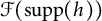
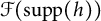
 $\mathcal {F}(\operatorname {\mathrm {supp}}(h))$
the future of the support of the initial condition.
In the example of the West Nile Virus model i, assuming that all nonzero atoms are supercritical, we deduce that starting with an initial condition where only the human population H is infected, the epidemic converges to the DFE and thus dies out, but starting with an initial condition where the populations H and M (or simply M or B) is infected, the epidemic converges to the unique EE
 $g^*$
, whose support is
 $\{B,M,H\}$
.
In the example of the zoonosis model ii, assuming again that all the atoms are supercritical, we deduce from Theorem 3, starting with an initial condition
 $u(0)=h$
, the epidemics converges in long time toward the equilibrium whose support is the support of h.
1.2.3 An algorithm to identify the support of the equilibrium
When
 $\Omega $
is a finite set, we provide a step by step procedure to compute the supercritical antichain related to the limit equilibrium for an initial condition
 $h \in \Delta $
given by Theorem 5.1. Recall Section 1.2, especially the definition of the transmission graph
 $G_K$
.
-
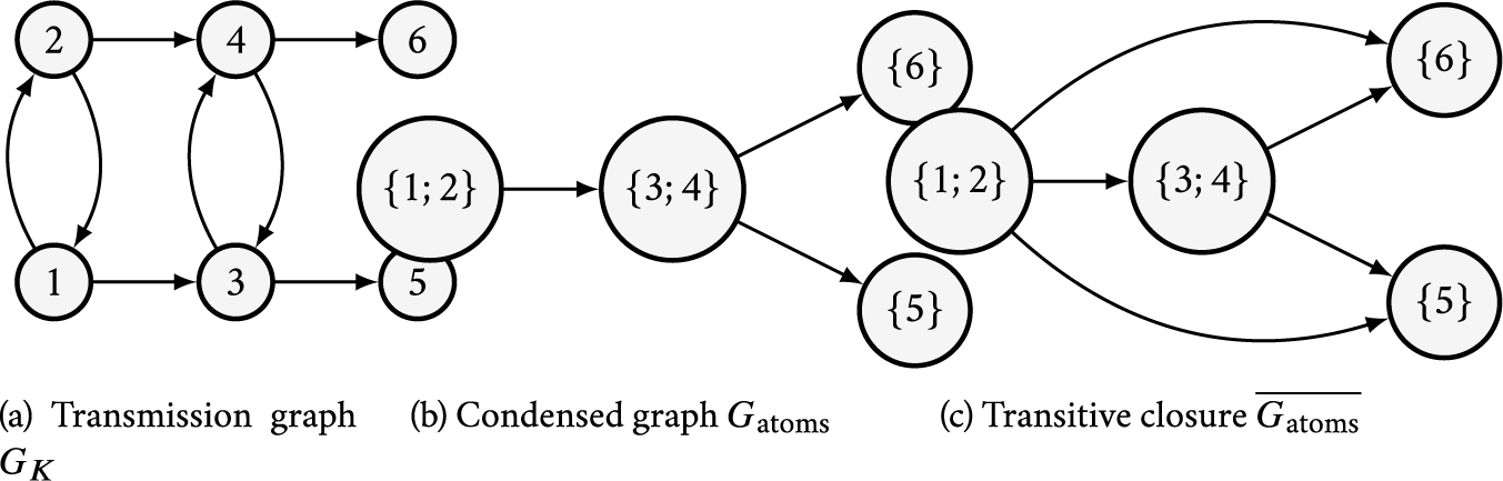
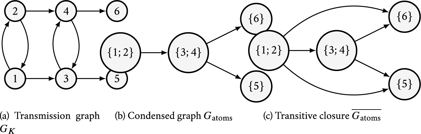
Find atoms: Starting from the transmission graph
$G_K$
, compute its condensation graph
$G_{\mathrm {atoms}}$
, whose vertices are the atoms of
$G_K$
, and there is a directed edge between atoms A and B if and only if, for some
$a\in A$
and
$b\in B$
,
$(ab)$
is an edge of
$G_K$
. Notice the condensation graph
$G_{\mathrm {atoms}}$
is finite. -
Find futures: Compute the transitive closure of
$G_{\mathrm {atoms}}$
: its vertices are the atoms, and there is an edge from A to B if and only if there is a path from A to B in
$G_{\mathrm {atoms}}$
(that is,
$B\preccurlyeq A$
and
$B\neq A$
). In particular, this allows for easy computation of futures: given any set, find all the atoms the set intersects, and take the union of all these atoms together with their outgoing neighbours in
$\overline {G_{\mathrm {atoms}}}$
. See Figure 2 for an example.Figure 2:An example of transmission graph
$G_K$
, its condensed graph
$G_{\mathrm {atoms}}$
and the transitive closure. -
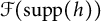
Identify supercritical atoms in
$\mathcal {F}(\operatorname {\mathrm {supp}}(h))$
: For each atom A that is included in
$\mathcal {F}(\operatorname {\mathrm {supp}}(h))$
, check whether
$R_0(A)$
is strictly greater than
$1$
(for example, by the power method). Define
$G_{\mathrm {supercrit}}$
the restriction of
$\overline {G_{\mathrm {atoms}}}$
to the supercritical atoms included in
$\mathcal {F}(\operatorname {\mathrm {supp}}(h))$
. -
Find the supercritical antichain related to the limit equilibrium: If
$G_{\mathrm {supercrit}}$
is empty, the limit equilibrium is the zero function
and its related supercritical antichain is empty. Otherwise, compute the supercritical antichain. This can, for example, be done in the following way: -
(1) initialize a set S to be all the vertices of
$G_{\mathrm {supercrit}}$
; -
(2) pick an element
$A\in S$
, and delete from S all outgoing neighbours of A; -
(3) iterate until all remaining elements of S have been treated.
-






Except for the last one, all steps in this procedure use classical algorithms that are easily found in graph libraries.
1.3 Assumptions and main results
Recall the SIS model (1.2) and (1.3) with parameter
 $(T, \gamma , \varphi )$
. We shall consider the following assumptions on the parameters. For
 $p\in [1, +\infty ]$
, let
 $L^p$
denote the usual Lebesgue space of measurable function defined on the measured space
 $(\Omega , \mathcal {G}, \mu )$
endowed with the
 $L^p$
norm
 $\left \lVert \,\cdot \,\right \rVert _p$
, and
 $L^p_+$
the subset of
 $L^p$
of nonnegative functions. Recall a linear map T on
 $L^p $
is positive if
 $T(L^p_+)\subset L^p_+$
.
Assumption 1 The measure
 $\mu $
is finite and nonzero; the map T is a bounded positive linear map on
 $L^\infty $
and there exists
 $p \in (1,+\infty )$
and a finite constant
 $C_p$
such that for all
 $f\in L^\infty $
:
 $$ \begin{align} \left\lVert\,Tf\,\right\rVert_p\leq C_p \, \left\lVert\,f\,\right\rVert_p; \end{align} $$
the function
 $\gamma $
belongs to
 $L^\infty $
and
 $\gamma>0,$
a.e.; and the function
 $\varphi : {\mathbb {R}} \rightarrow {\mathbb {R}}$
is locally Lipschitz, nonnegative on
 $[0, 1]$
and
 $\varphi (1) = 0$
.
Assumption 2 Assumption 1 holds; there exists a finite constant
 $C^{\prime }_p$
such that for all
 $f\in L^\infty $
:
 $$ \begin{align} \left\lVert\,Tf\,\right\rVert_\infty \leq C^{\prime}_p \, \left\lVert\,\gamma f\,\right\rVert_p; \end{align} $$
and the map
 $\varphi $
is decreasing on
 $[0,1]$
with
 $\varphi (0) = 1$
.
Remark 1.2 (On Conditions (1.5) and (1.6))
Block structured metapopulations can be represented using the finite setting of Section 1.2: the set
 $\Omega $
is finite, the operator T is given by a matrix and the function
 $\gamma $
is a positive vector. In this case, Conditions (1.5) and (1.6) always hold.
In the kernel model from Remark 1.1, if the kernel k is bounded and the function
 $\gamma $
is bounded away from 0, then, assuming that
 $\mu $
is finite, Conditions (1.5) and (1.6) hold. See also Remark 1.4 on the SIS model from [Reference Delmas, Dronnier and Zitt17].
The next two remarks are related to kernel operators. We also refer to Section 2.6 for further properties of the operator T induced by those two assumptions.
Remark 1.3 (The operator T is a kernel operator)
Assume Condition (1.6) holds. Since
 $\gamma $
is bounded, we deduce that there exists a finite constant
 $C^{\prime \prime }_p$
such that
 $\left \lVert \,Tf\,\right \rVert _\infty \leq C^{\prime \prime }_p \, \left \lVert \,f\,\right \rVert _p$
for all
 $f\in L^\infty $
, and also that Condition (1.5) holds. According to [Reference Schep49, Theorem 4.2], we deduce that T is a kernel operator (and the kernel is indeed nonnegative by Theorem 1.3 therein).
Remark 1.4 (The SIS model from [Reference Delmas, Dronnier and Zitt17])
Recall the definition of the kernel operator
 $T_k$
for k a kernel given in Section 1.1. We check that the SIS model from [Reference Delmas, Dronnier and Zitt17], see Assumption 1 therein, satisfies our Assumption 2. In [Reference Delmas, Dronnier and Zitt17], the measure
 $\mu $
is a probability measure on
 $\Omega $
, the function
 $\gamma $
is positive and bounded, and the mass-action incidence rate is associated with
 $\varphi = 1-\operatorname {\mathrm {Id}}$
. So the conditions on
 $\varphi $
,
 $\gamma $
, and
 $\mu $
in Assumption 2 are clearly satisfied. Therein, we have
 $T = T_k$
for
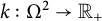 $k : \Omega ^2 \rightarrow {\mathbb {R}}_+$
a kernel such that
 $$ \begin{align} \sup_{x \in \Omega}\, \int_\Omega \left(\frac{k(x,y)}{\gamma(y)}\right) ^q \, \mu( \mathrm{d} y) < +\infty, \end{align} $$
for some
 $q\in (1, +\infty )$
. It is then elementary to check that the conditions on the operator
 $T=T_k$
from Assumption 2 are satisfied with
 $p \in (1,+\infty )$
given by
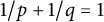 $1/p + 1/q = 1$
.
We now give our main results. Recall that
 $\Delta =\{f\in L_+^\infty \, \colon \, 1- f\in L^\infty _+\}$
is the set of measurable functions taking their value a.e. in
 $[0, 1]$
. Proposition 3.1 below asserts that under Assumption 1, for any initial condition
 $h \in \Delta $
, Equation (1.2) has a unique global solution in
 $L^\infty $
given by the semi-flow
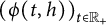 $\left (\phi (t, h)\right )_{t \in {\mathbb {R}}_+}$
and that
 $\phi (t, h)$
belongs to
 $\Delta $
for all
 $t\in {\mathbb {R}}_+$
. The following result on long time convergence appears below as Theorem 5.1 (see Section 2.3 below for a precise definition of the convergence involved).
Theorem 1 (Longtime behavior)
Let
 $(T, \gamma , \varphi )$
satisfy Assumption 2. The semi-flow
 $\phi $
always converges to an equilibrium: for any initial condition
 $h \in \Delta $
, there exists
 $g\in \Delta $
such that
 $F(g) = 0$
and
 $$ \begin{align} \operatorname*{\mbox{lim ess}}_{t \rightarrow + \infty} \phi(t, h) = g \quad\text{in } L^\infty. \end{align} $$
Under Assumption 2, we define the basic reproduction number
 $R_0$
as the spectral radius
 $\rho (T_{1/\gamma })$
of the power compact operator
 $T_{1/\gamma }$
on
 $L^\infty $
given by
 $T_{1/\gamma } f= T(f/\gamma )$
(see Lemma 2.8). It comes at no surprise that if
 $R_0\leq 1$
, then the zero function
 is the only equilibrium, so that all epidemic disappear in the long run (see Proposition 4.3). However, if
 , then there exists a maximal EE, say
 (see Theorem 4.7). If furthermore T is irreducible (which is equivalent to the existence and uniqueness, up to a scaling factor, of
 such that
 $Tv =R_0\, v$
and that v is positive), the maximal equilibrium
 $g^*$
is the only EE and g in (1.8) is equal to
 $g^*$
as soon as the initial condition h is nonzero (see again Proposition 4.3). Those results appear already in [Reference Delmas, Dronnier and Zitt17] in a slightly less general framework for
 $R_0\leq 1$
or T irreducible (or quasi-irreducible).
The main result of the article is the description of all the endemic equilibria and their domain of attraction: for any equilibrium g, we give all the initial conditions
 $h\in \Delta $
such that (1.8) holds. To do so, we shall rely on the decomposition of the state space in atoms associated with the operator T given by Schwartz [Reference Schwartz50], see also our previous work [Reference Delmas, Lefki and Zitt19], which is recalled in Section 2.4, and Section 1.2 for the elementary case where
 $\Omega $
is finite. To summarize, a measurable set
 $A \in \mathcal {G}$
is invariant if the support of the function
 is a subset of A (up to a set of zero measure); a set is admissible if it belongs to the
 $\sigma $
-field generated by the invariant sets; the atoms are the minimal admissible sets with positive measure (that is, A is an atom if A is admissible with
 $\mu (A)>0$
and if
 $B\subset A$
is admissible then either
 $\mu (B)=0$
or
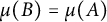 $\mu (B)=\mu (A)$
). If T is irreducible, then
 $\Omega $
is an atom. For a measurable set A, its future
 $\mathcal {F}(A)$
is the smallest invariant set containing A (up to a set of zero measure). The set of atoms (identifying atoms which differ by a set of zero measure) can be endowed with an order relation
 $\preccurlyeq $
:
 $A \preccurlyeq B$
when
 $\mathcal {F}(A) \subset \mathcal {F}(B)$
(where the inclusion holds up to a set of zero measure). See Section 2.4 for further details. We say that an atom A is supercritical if the spectral radius of the operator
 $T_{1/\gamma }$
restricted to A, denoted
 $R_0(A)$
, is strictly larger than
 $1$
. The number of supercritical atoms is finite; it is positive if and only if
 $R_0>1$
(see [Reference Delmas, Lefki and Zitt19]). A supercritical antichain is a finite set of supercritical atoms which are pairwise unordered with respect to
 $ \preccurlyeq $
; we define its future as the future of the union of its atoms. For example, with two supercritical atoms, say A and B, the supercritical antichains are
 $\emptyset $
,
 $\{A\},$
and
 $\{B\}$
, with also
 $\{A, B\}$
if A and B are unordered. Notice that
 $R_0>1$
if and only if there exists a non empty supercritical antichain.
We give a complete characterization of equilibria, see Theorem 4.8 for a more complete statement.
Theorem 2 (Equilibria and supercritical antichains are in bijection)
If
 $(T, \gamma , \varphi )$
satisfy Assumption 2, then the set of supercritical antichains and the set of equilibria are in bijection. Furthermore, the support of the equilibrium associated with a supercritical antichain is given by its future.
The empty supercritical antichain corresponds to the DFE
 . We deduce from this result that if g and
 $g'$
are two equilibria, then
 $g\leq g'$
if and only if
 $\operatorname {\mathrm {supp}}(g) \subset \operatorname {\mathrm {supp}}(g')$
(up to a set of zero measure) and
 $\operatorname {\mathrm {supp}}(h)=\{h>0\}$
is the support of the function h (see Corollary 4.2).
To complete this theorem we fully describe basins of attraction. To state the result, we denote by
 $T_A$
the projection of T on a measurable set A, that is, the operator on
 $L^\infty $
defined by
 for
 $f\in L^\infty $
. Notice that if T satisfies Assumption 2, so does
 $T_A$
. When this is the case, we say that g is the maximal equilibrium of A when g is the maximal equilibrium of the SIS model with T replaced by
 $T_A$
. Intuitively, from an initial condition
 $h\in \Delta $
, the epidemic converges to an equilibrium which depends only on the support of the initial condition; it is the same as the one starting from the “worst possible case” where the whole population in
 $\mathcal {F}(\operatorname {\mathrm {supp}}(h))\subset \Omega $
is infected.
Theorem 3 (Basins of attraction of equilibria)
The limiting equilibrium g of an epidemic with initial condition
 $h\in \Delta $
from Theorem 1 is the maximal equilibrium of
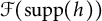 $\mathcal {F}(\operatorname {\mathrm {supp}}(h))$
.
This result appears below as Theorem 5.1. It is a full generalization of Theorem 4.13 in [Reference Delmas, Dronnier and Zitt17], which only covers the irreducible case T where, if
 $R_0>1$
, the EE g is unique and all epidemics with initial condition
 converge to g in large time. When
 $\operatorname *{\mbox {ess inf}} \gamma> 0$
, the epidemic converges uniformly to g, and to
 exponentially fast when furthermore
 $R_0<1$
(see Proposition 5.5). This uniform convergence is no longer true a priori when
 $\operatorname *{\mbox {ess inf}} \gamma = 0$
(see Remark 4.5 and Example 4.6).
1.4 Model with an external disease reservoir
We consider an infinite-dimensional SIS model with an external disease reservoir, called SIS
 $\kappa $
model in [Reference Nieddu, Forgoston and Billings42]; it can be seen as an extension of the SIS model (1.2). An external disease reservoir is a particular case of environmentally transmitted diseases where the population of pathogens in the environment is assumed to be constant over time(see, for example, [Reference Gerba23, Reference Lanzas, Davies, Erwin and Dawson34] and references therein). See also the example of the West Nile Virus, where birds and mosquitoes form a reservoir that is not infected by humans (see [Reference Bowman, Gumel, Van den Driessche, Wu and Zhu7]). It also encompasses some SIS models with immigration from [Reference Brauer and van den Driessche10] (see Remark 1.5 below).
Recall
 $I(t) \geq 0$
and
 $S(t) \geq 0$
denote, respectively, the number of infected individuals and susceptible individuals at time
 $t \geq 0$
. According to [Reference Nieddu, Forgoston and Billings42, Equation (2.1-2)], the corresponding ordinary differential equations model, including infection from the external disease reservoir, is given by
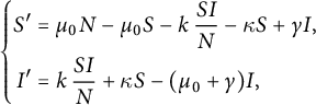 $$ \begin{align} \left\{ \begin{aligned} S'&= \mu_0 N - \mu_0 S - k \,\frac{SI}{N}- \kappa S +\gamma I,\\ I'&= k\, \frac{SI}{N} + \kappa S - (\mu_0 +\gamma) I, \end{aligned} \right. \end{align} $$
where
 $N=I+S$
is the total population,
 $\mu _0$
is the healthy birth rate and the common death rate of the susceptible and infected populations, and
 $\kappa S$
is the rate of disease transmission from the reservoir, with
 $\kappa>0$
. Notice the total size population N is constant in time.
In an inhomogeneous setting, with the measured space of types
 $(\Omega , \mathcal {G}, \mu )$
and
 $\mu (\Omega )\in (0, +\infty )$
, the proportion of infected individuals among the individuals with feature x is given by
 $u(t,x)=I(t,x)/N(x)$
, where
 $I(t,x)$
denotes the number of infected individuals with feature
 $x\in \Omega $
at time
 $t\in {\mathbb {R}}_+$
and
 $N(x)$
the total size of the population with feature
 $x \in \Omega $
, assumed constant over time. In the inhomogeneous SIS
 $\kappa $
model inspired by (1.9), the function
 $u=(u(t,x))_{t\in {\mathbb {R}}_+, x\in \Omega }$
is solution in
 $L^\infty $
of the ODE:
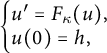 $$ \begin{align} \left\{\begin{array}{@{}l} u' = F_\kappa(u), \\ u(0) = h, \end{array}\right. \end{align} $$
with initial condition
 $h\in L^\infty $
and
 $$ \begin{align} F_\kappa(u)= \varphi(u) (Tu+\kappa) - \gamma u, \end{align} $$
where
 $\varphi $
is a continuous function on
 ${\mathbb {R}}$
and
 $\kappa \in L^\infty _+$
. The particular case of SIS
 $\kappa $
model given by (1.9) corresponds to
 $\Omega =\{\omega \}$
,
 $\mu $
a Dirac mass at
 $\omega $
, T the multiplication operator by k,
 $\gamma $
, and
 $\kappa $
constant functions, and
 $\varphi =1-\operatorname {\mathrm {Id}}$
.
This model can be related to SIS model with immigration, see the following remark.
Remark 1.5 (SIS model with immigration)
For the homogeneous population, we link the SIS
 $\kappa $
model (1.9) with the SIS model with immigration of [Reference Brauer and van den Driessche10, Equation (1)]. Assume initially that the total population
 $N(t)$
is not necessarily constant over time t. Let
 $A \geq 0$
be the immigration rate,
 $p \in [0,1]$
the proportion of infected individuals among the immigrants, and
 $d> 0$
the death rate among the population. All those parameters are assumed to be constant over time. We assume that the epidemic induces no death (that is,
 $\alpha = 0$
in [Reference Brauer and van den Driessche10, Equation (1)]) and that the incidence rate is the standard mass-action. Then, the SIS model with immigration given in [Reference Brauer and van den Driessche10, Equation (11)] reduces to
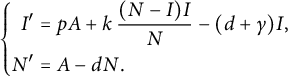 $$ \begin{align} \left\{ \begin{aligned} I' &= pA + k\, \frac{(N-I)I}{N} - (d+\gamma)I, \\ N' &= A - d N. \end{aligned} \right. \end{align} $$
Since
 $\lim _{t\rightarrow \infty } N(t)=A/d$
, and since we are interested in the long time equilibrium, it is natural to assume that N start at its equilibrium, that is,
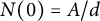 $N(0)=A/d$
, so that the population size is constant over time. In this case, Equation (1.12) with
 $u(t) = I(t)/N(0)$
reduces to
 $$ \begin{align} u' = (1-u)(ku+pd) - (\gamma + (1-p)d)u. \end{align} $$
The same arguments applied to an inhomogeneous population would lead to a similar multi/infinite-dimensional ODE with
 $u(t)$
replaced by a function
 $u(t,x)$
, with
 $x\in \Omega $
the set of features, and
 $ku$
replaced by
 $Tu$
with T the transmission operator, so that (1.13) becomes:
 $$\begin{align*}u' = (1-u)(Tu+pd) - (\gamma + (1-p)d)u. \end{align*}$$
This corresponds to the SIS
 $\kappa $
model (1.10) and (1.11) with
 $\varphi = 1-\operatorname {\mathrm {Id}}$
,
 $\kappa = pd$
, and
 $\gamma $
replaced by
 $\gamma + (1-p)d$
. In conclusion, the SIS model with immigration and the SIS model with an external disease reservoir lead to the same ODE.
In Proposition 6.1 and Corollary 6.2, we prove that the SIS
 $\kappa $
model with reservoir of (1.10) can be analyzed using the classical SIS model (1.2) by adding a new element
 ${\mathbf {r}}$
to the set of features
 $\Omega $
corresponding to the reservoir. In particular, we provide a full description of the equilibria and their domain of attraction for the SIS
 $\kappa $
model.
1.5 Discussion on the incidence rate
In this section, we discuss different models for the infection rate, and more precisely for the function
 $\varphi $
in (1.3).
In an homogeneous population, Ross [Reference Ross45] considered the so called law of mass action
 $\beta SI/N$
(which corresponds to
 $\varphi = 1-\operatorname {\mathrm {Id}}$
in the SIS model): the incidence rate is proportional to the product of the proportion of susceptible individuals and the proportion of infected individuals. According to Wilson and Worcester [Reference Wilson and Worcester57], it corresponds to the assumption that infected individuals are mixing uniformly with the susceptible ones throughout the population (see also Heesterbeek [Reference Heesterbeek26] for a historical review). Some epidemic models introduced in the literature replace the law of mass action by various incidence rates, see in particular the survey McCallum, Barlow and Homeo [Reference McCallum, Barlow and Hone38]. Concerning the function
 $\varphi $
, Assumptions 1 and 2 below reduce to
 $$ \begin{align} \varphi \text{ is locally Lipschitz on } {\mathbb{R}}, \text{ decreasing on } [0,1] \text{ with } \varphi(1) = 0 \text{ and } \varphi(0) = 1. \end{align} $$
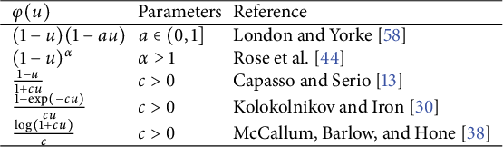
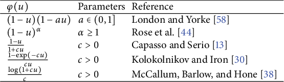
In the examples below from the literature, see Table 1, the set
 $\Omega $
is a singleton and the transmission operator T is thus a constant, which is assumed to be positive; so the condition
 $\varphi (0) = 1$
is a normalization convention on the (constant) operator T and could be replaced here by the more relevant condition
 $\varphi (0)>0$
.
-
(1) London and Yorke [Reference Yorke and London58] consider the incidence rate
$\beta SI(1 -cI)$
, that is, for measles epidemic (in New York City and Baltimore from 1928 to 1972) in order to eliminate the systematic differences on data observed between years with many cases and years with relatively few cases; however, they do not provide a biologic or physical argument for such modification. Notice that by considering
$$\begin{align*}\varphi(u) = (1-u)(1-au)\quad\text{with}\quad a>0 \end{align*}$$
$u/a$
instead of u, one can assume that
$a \leq 1$
, in which case Condition (1.14) holds.
-
(2) We recall that in the SIR model, once infected, the individuals recover with a permanent immunity. Rose et al. [Reference Rose, Medford, Goldsmith, Vegge, Weitz and Peterson44] incorporate in the SIR model (with constant population
$N=S+I+R$
) a population-level heterogeneity for the infection susceptibility given by the gamma probability distribution; in [Reference Rose, Medford, Goldsmith, Vegge, Weitz and Peterson44, Section 4], they consider the incidence rate
$\beta I S^\alpha $
. Using data from the 2009 H1N1 influenza outbreak, they observe that the higher-order models are more consistent with the data than the case
$\alpha =1$
. In our setting, this model would correspond to the following function
$\varphi $
with satisfies Condition (1.14):
$$\begin{align*}\varphi(u) = (1-u)^\alpha \quad\text{with}\quad \alpha\geq 1. \end{align*}$$
-
(3) Capasso and Serio [Reference Capasso and Serio13] study an SIR model (with constant population
$N=S+I+R$
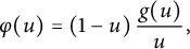
) taking into account saturation and “psychological” effects. They consider the incidence rate
$g(I)S$
. In our setting, this model would correspond to where the conditions on g translated into our framework correspond to: the function g is defined on
$$\begin{align*}\varphi(u) = (1-u)\, \frac{g(u)}{u}, \end{align*}$$
$[0,1]$
, nonnegative, bounded, differentiable with
$g'$
bounded and such that
$g(0) = 0$
,
$g'(0)=1$
and
$g(u) \leq u$
on
${\mathbb {R}}_+$
. Under those assumptions, the function
$\varphi $
is Lipschitz on
$[0,1]$
, with
$\varphi (1)=0$
and
$\varphi (0)=1$
. However, the monotonicity condition on
$\varphi $
on
$[0,1]$
, which amounts to
$g(u)\geq u(1-u) \, g'(u)$
on
$[0, 1]$
, is not satisfied in general.
Notice that Condition (1.14) is indeed satisfied for the following functions g, where
$c>0$
:
$u/(1+cu)$
in [Reference Capasso and Serio13, Section 6],
$(1-\exp (-cu))/c$
in [Reference Kolokolnikov and Iron30] on SIR model for Covid19 outbreak, and
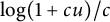
$\log (1+cu)/c$
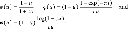
in Table 1 of the survey [Reference McCallum, Barlow and Hone38] on pathogen transmission models. They, respectively, correspond to
$$\begin{align*}\varphi(u) &= \frac{1-u}{1+cu}, \quad \varphi(u) = (1-u)\, \frac{1-\exp(-cu)}{cu} \quad\text{and}\quad \\ \varphi(u) &=(1-u) \, \frac{\log(1+cu)}{cu}\cdot \end{align*}$$
Table 1:Some popular choices for
$\varphi $
satisfying (1.14). -
(4) We recall that in the SIRS model, once infected, the individuals recover with a temporary immunity. To exhibit qualitatively different dynamical behaviors, Liu, Lewin, and Iwasa [Reference Liu, Levin and Iwasa35] introduced an SIRS model (with constant population
$N=S+I+R$
) where the incidence rate is given by
$ I H(I,S)$
for some differentiable function H such that
$H(I,0)=0$
and
$\partial _S H>0$
for all
$I>0$
. The latter condition reflects the biologically intuitive requirement that the incidence rate be an increasing function of the number of susceptibles. In our setting, this model would correspond to with
$$\begin{align*}\varphi(u)= H(u, 1-u), \end{align*}$$
$\varphi $
differentiable and
$\varphi (1)=0$
. Notice that
$\varphi $
is decreasing on
$[0,1]$
if
$\partial _S H> \partial _I H$
. The authors consider the particular case
$\varphi (u) = (1-u)^\alpha \, u^{\beta -1}$
with
$\alpha , \beta> 0$
. Condition (1.14) holds for
$\beta = 1$
and
$\alpha \geq 1$
, which is already considered in Point (2).
























2 Notations
2.1 Ordered set
Let
 $(E, \leq )$
be a (partially) ordered set. Whenever it exists, the supremum of
 $A\subset E$
, denoted by
 $\sup (A)$
, is the least upper bound of A: for all
 $x\in A$
,
 $x \leq \sup (A)$
and if for some
 $z\in E$
one has
 $x\leq z$
for all
 $x\in A$
, then
 $\sup (A) \leq z$
. A collection
 $(x_i)_{i \in \mathcal {I}}$
of elements of E is an antichain if for all distinct
 $i, j \in \mathcal {I}$
, the elements
 $x_i$
and
 $x_j$
are not comparable for the order relation.
2.2 Banach space and Banach lattice
Let
 $(X, \left \lVert \,\cdot \,\right \rVert )$
be a complex Banach space not reduced to
 $\{0\}$
. An operator T on X is a bounded linear (and thus continuous) map from X to itself. If
 $Y \subset X$
is a closed subspace of X such that
 $T(Y) \subset Y$
, we denote
 $T|_Y$
the restriction of T to the subspace Y, that is, an operator on the Banach space
 $(Y, \left \lVert \,\cdot \,\right \rVert )$
. The operator norm of T is given by
 $$ \begin{align} \left\lVert\,T\,\right\rVert_X= \sup\left\{ \left\lVert\,Tx\,\right\rVert\, \colon\, x \in X \text{ s.t. } \left\lVert\,x\,\right\rVert = 1\right\}, \end{align} $$
its spectrum by
 $\operatorname {\mathrm {Sp}}(T) = \{\lambda \in {\mathbb {C}}\, \colon \, T - \lambda \operatorname {\mathrm {Id}} \text { is not bijective}\}$
, where
 $\operatorname {\mathrm {Id}}$
is the identity operator on X. If
 $\lambda \in {\mathbb {C}}$
and
 $x\in X\backslash \{0\}$
satisfy
 $Tx=\lambda x$
, then the element x is an eigenvector of T and
 $\lambda $
, which belongs to
 $\operatorname {\mathrm {Sp}}(T) $
, is an eigenvalue of T. The spectral radius of T is defined by (see [Reference Rudin47, Theorem 18.9])
 $$ \begin{align} \rho(T) = \sup\left\{ |\lambda| \,\colon\, \lambda \in \operatorname{\mathrm{Sp}} (T)\right\} =\lim_{n\rightarrow \infty } \left\lVert\,T^n\,\right\rVert_X^{1/n}. \end{align} $$
By convention, we set
 $T^0=\operatorname {\mathrm {Id}}$
. The spectral radius is commutative in the sense that if T and S are two operators on X, we have
 $$ \begin{align} \rho(TS) = \rho(ST). \end{align} $$
We define the spectral bound of the operator T by
 $$ \begin{align} s(T) = \sup \{{\mathcal{R}e}(\lambda) \,\colon\, \lambda \in \operatorname{\mathrm{Sp}}(T)\}. \end{align} $$
Let
 $X^\star $
denote the (continuous or topological) dual Banach space of X, that is, the set of all the continuous linear forms on X. For
 $x\in X$
,
 $x^\star \in X^\star $
, let
 $\langle x^\star , x \rangle $
denote the duality product and the norm of
 $x^\star $
in
 $X^\star $
is defined by
 $\left \lVert \,x^\star \,\right \rVert =\sup \{\langle x^\star , x \rangle \, \colon \, \left \lVert \,x\,\right \rVert =1\}$
. For an operator T, the dual operator
 $T^\star $
on
 $X^\star $
is defined by
 $\langle T^\star x^\star , x \rangle =\langle x^\star , Tx \rangle $
for all
 $x\in X$
,
 $x^\star \in X^\star $
. It is well known that
 $\left \lVert \,T^\star \,\right \rVert _{X^\star }=\left \lVert \,T\,\right \rVert _X$
and
 $\operatorname {\mathrm {Sp}}(T^\star ) = \operatorname {\mathrm {Sp}}(T)$
.
An ordered real Banach space
 $(X, \left \lVert \,\cdot \,\right \rVert , \leq )$
is a real Banach space
 $(X, \left \lVert \,\cdot \,\right \rVert )$
with an order relation
 $\leq $
satisfying:
-
(1) for any
$x, y, z \in X, \lambda \geq 0$
such that
$x \leq y$
, we have
$x + z \leq y + z$
and
$\lambda x \leq \lambda y$
.




For any
 $x \in X$
, we define
 $|x| = \sup (\{x, -x\})$
the supremum of x and
 $-x$
whenever it exists. Following [Reference Schaefer48, Section 2], the ordered Banach space
 $(X, \left \lVert \,\cdot \,\right \rVert , \leq )$
is a Banach lattice if:
-
(1) for any
$x, y \in X$
, there exists a supremum of x and y in X; -
(2) for any
$x, y \in X$
so that
$|x| \leq |y|$
, we have
$\left \lVert \,x\,\right \rVert \leq \left \lVert \,y\,\right \rVert $
.


Let
 $(X, \left \lVert \,\cdot \,\right \rVert , \leq )$
be a real Banach lattice. We denote
 $X_+ = \{x \in X \,\colon \, x \geq 0 \}$
the positive cone of X. Recall it is a closed set. We shall also consider the dual cone
 $X^\star _+=\{x^\star \in X^\star \, \colon \, \langle x^\star , x \rangle \geq 0 \text { for all } x\in X_+\}$
. A linear map T on X is positive if
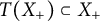 $T(X_+) \subset X_+$
. According to [Reference Aliprantis and Burkinshaw2, Theorem 4.3] positive linear maps on Banach lattices are bounded (and thus are operators).
If S and T are two operators on X, we write
 $T \leq S$
if the operator
 $S - T$
is positive. If the operators
 $T, S$
, and
 $S-T$
are positive, then we have, see [Reference Marek37, Theorem 4.2]:
 $$ \begin{align} \rho(T) \leq \rho(S). \end{align} $$
Any real Banach lattice X and any operator T on X admits a natural complex extension. The spectrum of T will be identified as the spectrum of its complex extension and denoted by
 $\operatorname {\mathrm {Sp}}(T)$
, furthermore, by [Reference Abramovich and Aliprantis1, Lemma 6.22], the spectral radius of the complex extension is also given by
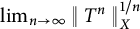 $\lim _{n\rightarrow \infty } \left \lVert \,T^n\,\right \rVert _X^{1/n}$
, with
 $\left \lVert \,\cdot \,\right \rVert _X$
still defined by (2.1). Moreover, by [Reference Abramovich and Aliprantis1, Corollary 3.23], if T is positive (seen as an operator on the real Banach lattice X), then T and its complex extension have the same norm.
2.3 Lebesgue spaces and essential limits
Let
 $(\Omega , \mathcal {G}, \mu )$
be a measured space with
 $\mu $
a finite measure. For any
 $\mathcal {A} \subset \mathcal {G}$
, we denote by
 $\sigma (\mathcal {A})$
the
 $\sigma $
-field generated by
 $\mathcal {A}$
. If f and g are two real-valued measurable functions defined on
 $\Omega $
, we write
 $f \leq g$
a.e. (resp.
 $f = g$
a.e.) when
 $\mu (\{f> g\}) = 0$
(resp.
 $\mu (\{f \neq g \}) = 0$
), and denote
 $\operatorname {\mathrm {supp}}(f )= \{f \neq 0\}$
the support of f. We say that a real-valued measurable function f is nonnegative when
 $f \geq 0$
a.e., we say that f is positive, denoted
 $f> 0$
a.e., when
 $\mu (\{f \leq 0\}) = 0$
, and we say that f is bounded if there exists
 $M \geq 0$
such that
 $|f| \leq M$
a.e. In what follows, the inclusion of measurable sets will be understood up to sets of
 $\mu $
-zero measure. More precisely, if
 $A, B \subset \Omega $
are measurable sets, we write
 $A \subset B$
a.e. (resp.
 $A = B$
a.e.) when
 a.e. (resp.
 a.e.). Let
 $L^0(\Omega , \mathcal {G}, \mu )$
, simply denoted
 $L^0$
, be the set of
 $[-\infty , + \infty ]$
-valued measurable functions defined on
 $\Omega $
, where functions which are a.e. equal are identified. The elements
 and
 of
 $L^0$
denote the functions which are a.e. equal, respectively, to 1 and to 0. For the sake of clarity, we will omit to write a.e. in the proofs.
Let
 $(f_t)_{t\in T}$
be a family of measurable functions defined on
 $\Omega $
taking values in
 $[-\infty , +\infty ]$
. We recall that
 $f^*=\operatorname *{\mbox {ess sup}}_{t\in T} f_t$
is a measurable function such that
 $f_t\leq f^*$
a.e. for all
 $t\in T$
and if f is measurable function such that
 $f_t\leq f$
a.e. for all
 $t\in T$
then
 $f ^*\leq f$
a.e. (if T is at most countable, then one can take
 $\operatorname *{\mbox {ess sup}}_{t\in T} f_t=\sup _{t\in T} f_t$
). We now consider
 $T={\mathbb {R}}_+$
. Let
 $(f_t)_{ t\in {\mathbb {R}}_+}$
be a non-decreasing family, in the sense that for all
 $t\leq s$
we have
 $f_t\leq f_s$
a.e., then if
 $(t_n)_{ n\in {\mathbb {N}}}$
is a sequence converging to
 $+\infty $
, we have that the sequence
 $(f_{t_n})_{ n\in {\mathbb {N}}}$
converges a.e. toward
 $f^*=\operatorname *{\mbox {ess sup}}_{t\in {\mathbb {R}}_+} f_t$
, and thus we shall simply write
 $f^*=\operatorname *{\mbox {lim ess}}_{t\rightarrow +\infty } f_t$
. We leave to the reader the definition of
 $\operatorname *{\mbox {ess inf}}$
and the limit of a non-increasing sequence of measurable functions. For the family
 $(f_t)_{ t\in {\mathbb {R}}_+}$
, we consider
 $f^*_t=\operatorname *{\mbox {ess sup}}_{s\geq t} f_s$
for all
 $t\in {\mathbb {R}}_+$
, and get that the sequence
 $(f^*_t)_{t\in {\mathbb {R}}^+}$
is non-increasing and write
 $\operatorname *{\mbox {lim ess sup}}_{t\rightarrow \infty } f_t= \operatorname *{\mbox {lim ess}}_{t\rightarrow \infty } f^*_t$
. We define in a similar way
 $\operatorname *{\mbox {lim ess inf}}_{t\rightarrow \infty } f_t$
. Notice that if
 $g_t=f_t$
a.e. for all
 $t\in {\mathbb {R}}_+$
, then the essential supremum/infimum limits of
 $(f_t)_{t\in {\mathbb {R}}^+}$
and
 $(g_t)_{t\in {\mathbb {R}}^+}$
are a.e. equal. Therefore, the essential supremum/infimum limits of sequences is well defined on the space
 $L^0$
. We say the sequence of functions
 $(f_t)_{ t\in {\mathbb {R}}_+}$
in
 $L^0$
essentially converges if
 $\operatorname *{\mbox {lim ess sup}}_{t\rightarrow \infty } f_t=\operatorname *{\mbox {lim ess inf}}_{t\rightarrow \infty } f_t$
in
 $L^0$
, and write
 $\operatorname *{\mbox {lim ess}}_{t\rightarrow +\infty } f_t$
for this common limit (which is an element of
 $L^0$
). When considering
 $T={\mathbb {N}}$
instead of
 $T={\mathbb {R}}_+$
, the analog of the essential convergence is the a.e. convergence, that is, the usual convergence in
 $L^0$
.
For a measurable function f, we write
 $\mu (f)=\int f\, \mathrm {d} \mu =\int _\Omega f(x)\, \mu (\mathrm {d} x)$
the integral of f with respect to
 $\mu $
when it is well defined. When f is measurable and a.e. finite and nonnegative, we denote
 $f \mu $
the measure on
 $(\Omega , \mathcal {G})$
defined by
 for any measurable set A. For
 , the Lebesgue space
 $L^p(\Omega , \mathcal {G}, \mu )$
is the set of all real-valued measurable functions
 $f\in L^0$
defined on
 $\Omega $
whose
 $L^p$
-norm,
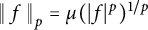 $\left \lVert \,f\,\right \rVert _p = \mu (|f|^p)^{1/p}$
if
 $p<+\infty $
and
 $\left \lVert \,f\,\right \rVert _\infty = \operatorname *{\mbox {ess sup}}(|f|)$
if
 $p=+\infty $
, is finite. When there is no ambiguity we shall simply write
 $L^p(\Omega )$
,
 $L^p(\mu )$
or
 $L^p$
for
 $L^p(\Omega , \mathcal {G}, \mu )$
. The Banach space
 $L^p$
endowed with the usual order
 $f\leq g$
, that is,
 $\mu (\{f>g\})=0$
, is a Banach lattice. The positive cone
 $L^p_+$
is the subset of
 $L^p$
of nonnegative functions; it is normal (as the norm
 $\left \lVert \,\cdot \,\right \rVert $
is monotonic, that is,
 $0\leq f\leq g$
implies
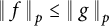 $\left \lVert \,f\,\right \rVert _p\leq \left \lVert \,g\,\right \rVert _p$
, see [Reference Deimling15, Proposition 19.1]) and reproducing (that is,
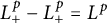 $L^p_+ -L^p_+=L^p$
). Since the supports of two functions, which are a.e. equal are also a.e. equal, we get that the support of
 $f\in L^p$
is well defined up to the a.e. equality; it will still be denoted by
 $\operatorname {\mathrm {supp}}(f)$
. For
 $p\in [1, +\infty )$
, the dual of
 $L^p$
is
 $L^q$
where
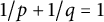 $1/p+1/q=1$
, with the duality product
 $\langle g, f \rangle = \int fg\, \mathrm {d} \mu $
for
 $f \in L^p$
and
 $ g \in L^q$
(for
 $p=1$
, we use that the measure
 $\mu $
is finite).
For any
 $f \in L^\infty $
, we denote by
 $M_f$
the multiplication by f, which can be seen as an operator on
 $L^p$
for
 $p \in [1,+\infty ]$
. For
 $A \in \mathcal {G}$
a measurable set, we denote:

Let T be an operator on
 $L^p$
. The projection of T on A, denoted
 $T_A$
, is the operator defined by
 $$ \begin{align} T_A=M_A \, T\, M_A, \end{align} $$
and, if
 $\mu (A)>0$
, we denote by
 $T|_A$
the restriction of the operator
 $T_A$
to
 $L^p(A)$
, where the set A is endowed with the trace of
 $\mathcal {G}$
on A and the measure
 $\mu |_A (\cdot )=\mu (A\cap \cdot )$
.
We now assume that
 $\mu (\Omega )>0$
, so that
 $L^p(\Omega )$
is not reduced to a singleton. When there is no ambiguity on the operator T, we simply write
 $\rho (A)$
for the spectral radius of
 $T_A$
(and of
 $T|_A$
when
 $\mu (A)>0$
). In particular, we have
 $\rho (\Omega )=\rho (T)$
and
 $\rho (A) = 0$
if
 $\mu (A) = 0$
. If the operator T is positive, we also have that
 $$\begin{align*}A \subset B \quad \Longrightarrow \quad \rho(A) \leq \rho(B). \end{align*}$$
2.4 Decomposition of positive operators on
$L^p$
, with
$p\in (1,+\infty )$


Recall the measure
 $\mu $
is finite and nonzero. We recall the atomic decomposition from Schwartz [Reference Schwartz50] of a positive operator T on
 $L^p$
(see also [Reference Delmas, Lefki and Zitt19]). A measurable set
 $A \in \mathcal {G}$
is T-invariant, or simply invariant when there is no ambiguity, if
 $M_{A^c} T M_A = 0$
, which, see [Reference Delmas, Lefki and Zitt19, Equation (7)], is equivalent to
 $$ \begin{align} \langle g , Tf \rangle=0, \end{align} $$
for all
 $f \in L^p_+$
and
 $ g \in L^q_+$
such that
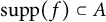 $\operatorname {\mathrm {supp}}(f) \subset A$
a.e. and
 $\operatorname {\mathrm {supp}}(g) \subset A^c$
a.e. The operator T is irreducible if its only invariant sets are a.e. equal to
 $\Omega $
or
 $\emptyset $
. A measurable set A with positive measure is irreducible if the operator
 $T|_A$
on
 $L^p(A)$
is irreducible. The future of a set
 $A \subset \Omega $
, denoted
 $\mathcal {F}(A)$
, is the smallest invariant set that contains A. If
 $\mathcal {C}$
is an at most countable collection of subsets of
 $\Omega $
, then we denote by
 $\mathcal {F}(\mathcal {C})$
the future of the union of the elements of
 $\mathcal {C}$
:
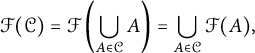 $$ \begin{align} \mathcal{F}(\mathcal{C})= \mathcal{F}\left( \bigcup_{A\in \mathcal{C}} A\right) = \bigcup_{A\in \mathcal{C}} \mathcal{F}(A), \end{align} $$
where the last equality is [Reference Delmas, Lefki and Zitt19, Lemma 3.13].
A set is admissible if it belongs to the
 $\sigma $
-field generated by the invariant sets. An atom is a minimal admissible set with a positive measure (that is, A is an atom if A is admissible,
 $\mu (A)>0$
and if B is an admissible set such that
 $B\subset A$
a.e. then a.e.
 $B=\emptyset $
or
 $B=A$
), and we identify two atoms that are a.e. equal. In particular, if the set A is an atom and B is admissible then we have
 $$\begin{align*}\mu(A \cap B)>0 \implies A\subset B \quad\text{a.e.} \end{align*}$$
According to [Reference Delmas, Lefki and Zitt19, Theorem 1], a measurable set is admissible and irreducible with positive measure if and only if it is an atom. Since the atoms have positive measure, we get that the set of atoms (up to the a.e. equality),
 $\mathfrak {A}$
, is at most countable. We shall also consider the (at most countable) set of nonzero atoms:
 $$\begin{align*}\mathfrak{A}^*=\{ A \in \mathfrak{A}\, \colon\, \rho(A)>0\}. \end{align*}$$
The relation
 $\preccurlyeq $
on
 $\mathfrak {A}$
, defined by
 $A \preccurlyeq B$
if
 $\mathcal {F}(A) \subset \mathcal {F}(B)$
a.e. (or equivalently
 $A \subset \mathcal {F}(B)$
a.e.) is an order relation. We end this section by noticing that antichains of atoms are characterized by their future.
Lemma 2.1 (Antichains with same future)
Let
 $\mathcal {C}$
and
 $\mathcal {C}'$
be two antichains of atoms. Then, we have
 $$\begin{align*}\mathcal{F}(\mathcal{C})=\mathcal{F}(\mathcal{C}')\quad \Longleftrightarrow \quad \mathcal{C}=\mathcal{C}'. \end{align*}$$
Proof Assume that
 $ \mathcal {F}(\mathcal {C})=\mathcal {F}(\mathcal {C}')$
. Consider an atom
 $A\in \mathcal {C}$
. Since
 $A\subset \mathcal {F}(\mathcal {C}) = \mathcal {F}(\mathcal {C}')$
, there exists
 $A' \in \mathcal {C}'$
such that we have
 $\mu (A \cap \mathcal {F}(A'))> 0$
, which implies
 $A \preccurlyeq A'$
as A is an atom. Conversely, there exists
 $B\in \mathcal {C}$
such that
 $A'\preccurlyeq B$
, and by transitivity
 $A\preccurlyeq B$
. Since
 $\mathcal {C}$
is an antichain, we obtain
 $A=B$
and thus
 $A=A'$
is an element of
 $\mathcal {C}'$
. The reverse implication is trivial by (2.9).
2.5 Power compact operators on
$L^p$

A linear map T on a Banach space is compact if the image of the unit ball is relatively compact; it is then bounded. An operator T on a Banach space is power compact if there exists
 $k \in {\mathbb {N}}^*$
such that
 $T^k$
is compact. We recall some well-known properties of power compact operators (see [Reference Dunford and Schwartz21, Reference König31] for instance).
Lemma 2.2 (Spectrum of power compact operators)
Let T be an operator on a Banach space.
-
(1) The operator
$T^\star $
is power compact if and only if the operator T is power compact. -
(2) If T is power compact, then the set
$\operatorname {\mathrm {Sp}}(T)$
is at most countable and has no accumulation points except possibly
$0$
(it is thus totally disconnected).


It is well known that the spectral radius (and more generally the spectra) is a continuous function on the set of compact operators with respect to the operator norm (see [Reference Newburgh41, Theorem 11]). We shall, however, use a weaker result from Anselone [Reference Anselone3]. We say a family
 $\mathcal {V}$
of operators on X is collectively compact if
 $\bigcup _{V\in \mathcal {V}} V(B)$
is relatively compact, where B is the unit ball of X. The following result is a direct consequence of Proposition 4.1 and Theorem 4.16 in [Reference Anselone3].
Lemma 2.3 (Collectively compact operators)
Let I be an interval of
 ${\mathbb {R}}$
and
 $(V_t)_{t\in I}$
be a family of collectively compact operators on a Banach space X. If
 $t\in I$
is such that
 $\lim _{s\rightarrow t} \left \lVert \,(V_s -V_t)x\,\right \rVert =0$
for all
 $x\in X$
, then we have
 $\lim _{s\rightarrow t}\rho (V_s)=\rho (V_t)$
.
We give a result on compact operators in Lebesgue space. Recall that
 $\mu $
is a nonzero finite measure on
 $\Omega $
, and that
 $L^p$
denote
 $L^p(\Omega , \mathcal {G}, \mu )$
.
Lemma 2.4 (On compactness)
Let
 $p \in (1,+\infty )$
. A positive operator on
 $L^p$
which is dominated by a compact operator is compact.
Proof Notice that
 $L^p$
has an order continuous norm for
 $p\in [1, \infty )$
, see [Reference Aliprantis and Burkinshaw2, Definition 4.7], that is, according to [Reference Aliprantis and Burkinshaw2, Theorem 4.9], if
 $(f_n)_{n\in {\mathbb {N}}}$
is a non-decreasing sequence of
 $L^p_+$
such that
 $\sup _{n\in {\mathbb {N}}} f_n=f\in L^p$
, then
 $\lim _{n\rightarrow \infty } \left \lVert \,f_n-f\,\right \rVert _p=0$
. In particular, when
 $p \in (1,+\infty )$
, the dual of
 $L^p$
, that is isomorphic to
 $L^q$
with
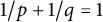 $1/p + 1/q = 1$
, also has an order continuous norm. The lemma is then a direct consequence of [Reference Aliprantis and Burkinshaw2, Theorem 5.20].
We recall in our framework some classical results, see [Reference Delmas, Lefki and Zitt19, Theorem 6.2 and Lemma 6.5].
Theorem 2.5 Let T be a positive power compact operator on
 $L^p$
with
 $p \in (1,+\infty )$
.
-
(1) Krein–Rutman: If
$\rho (T)$
is positive then
$\rho (T)$
is an eigenvalue of T, and there exists a corresponding nonnegative right eigenfunction denoted
$v_T$
. -
(2) de Pagter: If T is irreducible then
$\rho (T)$
is positive unless
$T=0$
and
$\dim (L^p)=1$
, that is, if A is measurable then either
$\mu (A)=0$
or
$\mu (A^c)=0$
. -
(3) Schwartz: We have that for any admissible set A:
(2.10)
$$ \begin{align} \rho(A)=\max_{B\in \mathfrak{A}^*, \, B\subset A} \rho(B). \end{align} $$


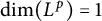



Following [Reference Delmas, Dronnier and Zitt18, Lemma 4.2], we now state a technical result based on Collatz–Wielandt inequality and the Krein–Rutman theorem, giving a bound on the spectral radius given a strict supersolution of the eigenvalue equation.
Lemma 2.6 (Supersolutions and spectral radius)
Let S be a positive operator on
 $L^p$
with
 $p \in (1, + \infty )$
. If there exists
 $\lambda>0$
and a non-null nonnegative function
 $v \in L^p_+$
such that
 $Sv \geq \lambda v$
, then:
 $$\begin{align*}\rho(S)\geq \rho(S_A) \geq \lambda, \end{align*}$$
where
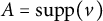 $A=\operatorname {\mathrm {supp}}(v)$
. Furthermore, if S is power compact, then we have
-
(1) If
$Sv= \lambda v$
on A, then
$\rho (S_A) = \lambda $
. -
(2) If
$Sv - \lambda v$
is positive on A, then
$\rho (S_A)> \lambda $
.


Proof We first note that
 $\rho (S)\geq \rho (S_A)$
by (2.5). Multiplying the inequality
 $Sv\geq \lambda v$
by
 yields that
 $S_A v \geq \lambda v$
. The fact that
 $\rho (S_A)\geq \lambda $
, and thus
 $\rho (S) \geq \lambda $
, is then a direct consequence of the Collatz–Wielandt inequality [Reference Förster and Nagy22, Propositions 2.1 and 2.2].
We now assume that S is power compact. Since
 $(S_A)^\star = (S^\star )_A$
, we shall denote them simply by
 $S^\star _ A$
. Since
 $S_A\leq S$
, we deduce from Lemma 2.4 that the operator
 $S_A$
, and thus
 $S_A^\star $
, is power compact. We apply the Krein–Rutman theorem (Theorem 2.5 (1)) to the power compact operator
 $S_A^\star $
, which has a positive spectral radius
 $\rho (S_A^\star ) = \rho (S_A)>0$
: there exists
 $w \in L^q_+$
a non-null eigenfunction of
 $S_A^\star $
related to the eigenvalue
 $\rho (S_A)$
. Since
 , we deduce that
 $\operatorname {\mathrm {supp}}(w) \subset A$
and thus
 $\langle w,v \rangle>0$
.
We now consider the following duality product:
 $$ \begin{align} \left\langle w,S_Av - \lambda v\right\rangle = \left\langle S_A^\star w,v\right\rangle - \lambda\left\langle w,v\right\rangle = (\rho(S_A) - \lambda)\left\langle w,v\right\rangle. \end{align} $$
Under the hypothesis that
 $Sv = \lambda v$
on
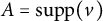 $A=\operatorname {\mathrm {supp}}(v)$
, the left-hand side of (2.11) is zero, and thus
 $\rho (S_A)=\lambda $
. This gives Point (1).
To prove Point (2), since
 $S_Av-\lambda v$
is by hypothesis positive on A, and
 is nonnegative and not identically equal to zero, we get
 $\left \langle w,S_Av - \lambda v\right \rangle>0$
. Then use (2.11) again to get that
 $\rho (S_A)>\lambda $
.
2.6 Operators related to the SIS model
Let
 $(\Omega , \mathcal {G}, \mu )$
be a measured space with finite nonzero measure
 $\mu $
, that is,
 $\mu (\Omega )\in (0, +\infty )$
. Recall we simply write
 $L^p$
for
 $L^p(\Omega , \mathcal {G}, \mu )$
. Observe that
 $L^\infty \subset L^p$
for
 $p \in (1,+\infty )$
and that the identity map
 $\iota $
from
 $L^\infty $
to
 $L^p$
is a bounded injection.
Lemma 2.7 (On compactness)
Let
 $p \in (1,+\infty )$
. Let T be an operator from
 $L^p$
to
 $L^\infty $
. The linear map
 $\iota T$
is a compact operator on
 $L^p$
.
Proof Since
 $L^p$
is reflexive, see [Reference Dunford and Schwartz21, Corollary IV.8.2], we get by [Reference Dunford and Schwartz21, Corollary VI.4.3] that T and
 $\iota $
are weakly compact. By [Reference Aliprantis and Burkinshaw2, Theorem 5.85], as the space
 $L^\infty $
is an AM-space (see [Reference Aliprantis and Burkinshaw2, Definition 4.20]), it satisfies the Dunford–Pettis property, thus, by [Reference Aliprantis and Burkinshaw2, Theorem 5.87], the operator
 $\iota T$
on
 $L^p$
is then compact.
Let
 $p\in (1, +\infty )$
and
 $\gamma \in L^\infty $
such that
 $\gamma>0$
a.e. Let T be a positive operator on
 $L^\infty $
such that (1.5) holds for all
 $f\in L^\infty $
. In particular, as
 $L^\infty $
is dense in
 $L^p$
(for the
 $L^p$
-norm), we can extend T by density into a bounded linear map
 $\hat {T}$
on
 $L^p$
. Recall that
 $M_{1/\gamma }$
denotes the multiplication by
 $1/\gamma $
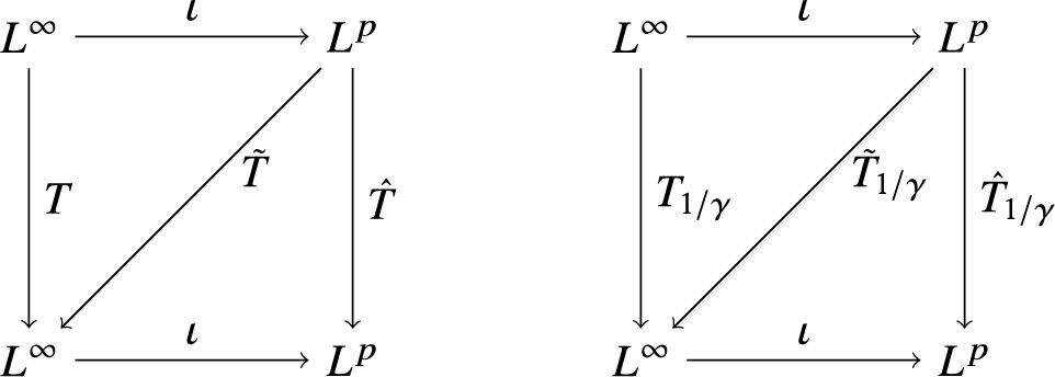
. Notice that under Assumption 2, see (1.6), the linear map
 $TM_{1/\gamma }$
, denoted by
 $T_{1/\gamma }$
, can be seen as a bounded linear map on
 $L^\infty $
, and it can also be extended by density into a bounded linear map
 $\hat {T}_{1/\gamma }$
on
 $L^p$
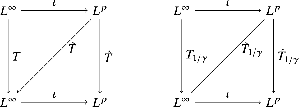
(see also Figure 3).
Operators related to T in the SIS model
 $(T, \gamma , \varphi )$
.
Lemma 2.8 (Properties of operators related to T)
Let
 $(T, \gamma , \varphi )$
satisfy Assumption 1. Then,
 $\hat {T}$
is an operator on
 $L^p$
. If Assumption 2 holds, then we have
-
(1)
$\hat {T}$
is a compact operator on
$L^p$
; -
(2)
$T^2$
is a compact operator on
$L^\infty $
; -
(3)
$\hat {T}_{1/\gamma }$
is a compact operator on
$L^p$
; -
(4)
$T_{1/\gamma }$
is an operator on
$L^\infty $
and
$T_{1/\gamma }^2$
is compact; -
(5)
$ \operatorname {\mathrm {Sp}}(T)=\operatorname {\mathrm {Sp}}(\hat {T})$
and
$ \operatorname {\mathrm {Sp}}(T_{1/\gamma })=\operatorname {\mathrm {Sp}}(\hat {T}_{1/\gamma })$
.




Proof Suppose Assumption 2 holds. We deduce from (1.6) that there exists a finite constant C such that
 $\left \lVert \,Tf\,\right \rVert _\infty \leq C \, \left \lVert \,f\,\right \rVert _p$
for all
 $f\in L^\infty $
. By density, we can extend T into an operator
 ${\tilde {T}}$
from
 $L^p$
to
 $L^\infty $
. This gives that
 $\hat {T}=\iota \, {\tilde {T}}$
and Point (a) on the compactness property of
 $\hat {T}$
is a consequence of Lemma 2.7. As
 $T= {\tilde {T}}\, \iota $
and thus
 $T^2= {\tilde {T}} \, \hat {T} \, \iota $
, we also get that
 $T^2$
is compact, that is, Point (b). Using (1.6), we can also extend
 $TM_{1/\gamma }$
into an operator
 ${\tilde {T}}_{1/\gamma }$
from
 $L^p$
to
 $L^\infty $
. Arguing as above gives Points (c) and (d).
We now prove Point (e). Two complex Banach spaces
 $(E, \left \lVert \,\cdot \,\right \rVert )$
and
 $(E', \left \lVert \,\cdot \,\right \rVert ')$
are compatible if
 $(E", \left \lVert \,\cdot \,\right \rVert + \left \lVert \,\cdot \,\right \rVert ')$
, with
 $E"=E\cap E'$
, is a Banach space, and
 $E"$
is dense in E and in
 $E'$
. Given two compatible spaces E and
 $E'$
, two operators A on E and
 $A'$
on
 $E'$
are said to be consistent if
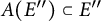 $A(E")\subset E"$
,
 $A'(E")\subset E"$
, and
 $Ax=A'x$
for all
 $x\in E"$
. If furthermore A and
 $A'$
are compact, then [Reference Davies14, Theorem 4.2.15] gives that
 $\operatorname {\mathrm {Sp}}(A)=\operatorname {\mathrm {Sp}}(A')$
. The proof therein relies on the spectrum to be at most countable and with no accumulation points except possibly
 $0$
and that the spectral projections have finite rank (see Theorems 5 and 6 p.579 in [Reference Dunford and Schwartz21]). Since this also holds for power compact operators, the results can be extended to A and
 $A'$
being power compact operators.
As
 $\mu $
is a finite measure, the spaces
 $L^p$
and
 $L^\infty $
are pairwise compatible. Notice also the operators T and
 $\hat {T}$
, as well as
 $T_{1/\gamma }$
and
 $\hat {T}_{1/\gamma }$
, are consistent. Then the equalities follow.
3 Equilibria and restriction
We consider the SIS model (1.2) and (1.3) on
 $L^\infty =L^\infty (\Omega , \mathcal {G}, \mu )$
with parameter
 $(T, \gamma , \varphi )$
such that Assumption 1 holds. In particular, the measure
 $\mu $
is finite and nonzero. We consider the following subset of
 $L^\infty $
:

Recall that g is an equilibrium if g belongs to
 $\Delta $
and solves (1.4), that is:
 $$\begin{align*}F(g)=0. \end{align*}$$
In particular, the function

is an equilibrium. We say that
 $g^*\in L^\infty $
is the maximal equilibrium if
 $g^*$
is an equilibrium and all other equilibrium
 $g\in L^\infty $
are such that
 $g\leq g^*$
.
The existence result of the semi-flow and the maximal equilibrium follows [Reference Delmas, Dronnier and Zitt17, Propositions 2.7 and 2.15] with slightly more general hypothesis on T and is obtained similarly, see a proof in Section 8 for completeness. We shall refer to this section for notations and definitions/properties of the semi-flow.
Proposition 3.1 (Existence of a global solution and of the maximal equilibrium)
Let
 $(T, \gamma , \varphi )$
be parameters of the SIS model satisfying Assumption 1. The following properties hold.
-
(1) Equation (1.2) in
$L^\infty $
with initial condition
$h\in \Delta $
has a unique global solution given by the semi-flow
$\phi (\cdot , h)=(\phi (t, h))_{t\in {\mathbb {R}}_+}$
. The semi-flow belongs to
$\mathcal {C}^1({\mathbb {R}}_+)$
. -
(2) For all
$t \geq 0$
and
$h \in \Delta $
, we have
$\phi (t, h) \in \Delta $
. -
(3) The sequence
is non-increasing and converges essentially to a limit,
$ g^*$
, which is the maximal equilibrium:





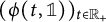


The convergence in Point (3) is not uniform in general, see Remarks 4.4 and 4.5 and Example 4.6.
The proof of the monotonicity of the maximal equilibrium in the parameters is given in Section 8 for consistency of the arguments.
Lemma 3.2 (Monotonicity of the maximal equilibrium)
For
 $i=1,2$
, let
 $(T_i, \gamma _i, \varphi _i)$
be parameters of the SIS model satisfying Assumption 1 and denote
 $g^*_i$
the corresponding maximal equilibrium. If
 $T_1 \geq T_2$
,
 $\varphi _1 \geq \varphi _2$
and
 $\gamma _1 \leq \gamma _2$
, then we have
 $g^*_1 \geq g^*_2$
.
Let A be a measurable set. Since
 $(T, \gamma , \varphi )$
satisfy Assumption 1, so does
 $(T_A, \gamma , \varphi )$
, where
 $T_A= T_A = M_A T M_A$
is the projection of T on A. We shall now focus on this restricted
 $(T_A, \gamma , \varphi )$
-SIS model. We set for
 $u\in L^\infty $
:
 $$ \begin{align} F_A(u) = \varphi(u) T_A(u) - \gamma u, \end{align} $$
and call
 $g\in \Delta $
an equilibrium of A if
 $F_A(g)=0$
. In this case, notice that
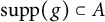 $\operatorname {\mathrm {supp}}(g) \subset A$
a.e. We also denote
 $\phi _A$
the corresponding semi-flow and
 $g^*_A$
the corresponding maximal equilibrium of A given by Proposition 3.1.
Lemma 3.3 (Maximal equilibria)
Let
 $(T, \gamma , \varphi )$
satisfy Assumption 1. Let
 $A\subset B$
a.e. be measurable sets. We have
 $g^*_A\leq g^*_B$
.
Proof Apply Lemma 3.2 with
 $T_1 = T_B\geq T_A=T_2$
,
 $\varphi _1 = \varphi _2 = \varphi $
and
 $\gamma _1 = \gamma _2 = \gamma $
.
We now provide results on equilibria and semi-flows associated with T and
 $T_A$
.
Lemma 3.4 (Equilibrium and restriction)
Let
 $(T, \gamma , \varphi )$
satisfy Assumption 1. Let A be a measurable set and
 $g \in \Delta $
.
-
(1) If g is an equilibrium and
$\operatorname {\mathrm {supp}}(g)\subset A $
a.e., then g is an equilibrium of A. -
(2) If A is invariant and g is an equilibrium of A, then g is an equilibrium (and
$\operatorname {\mathrm {supp}}(g)\subset A $
a.e.). -
(3) If A is invariant and g is an equilibrium, then
is an equilibrium of
$A^c$
and of
$A^c \cap \operatorname {\mathrm {supp}}(g)$
.
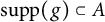
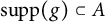



Proof If
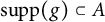 $\operatorname {\mathrm {supp}}(g)\subset A $
and g is an equilibrium, then we get that g is an equilibrium of A as

Let A be an invariant set and
 $h\in \Delta $
. Since
 , we deduce that

If furthermore
 $\operatorname {\mathrm {supp}}(h)\subset A$
, then we have

If g is an equilibrium of A, then we get
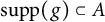 $\operatorname {\mathrm {supp}}(g)\subset A$
and, since A is invariant, we deduce from (3.3) that g is an equilibrium. If g is an equilibrium, we deduce from (3.2) that
 is an equilibrium of
 $A^c$
. Then, use (1) with T replaced by
 $T_{A^c}$
and A by
 $\operatorname {\mathrm {supp}}(g)$
to deduce that
 is also an equilibrium of
 $A^c \cap \operatorname {\mathrm {supp}}(g)$
.
Lemma 3.5 (Semi-flow and restriction)
Let
 $(T, \gamma , \varphi )$
satisfy Assumption 1. Let A be a measurable set and
 $h \in \Delta $
. The following properties hold:
-
(1)
. -
(2) If A is invariant, then we have
. -
(3) If A is invariant and
$\operatorname {\mathrm {supp}}(h) \subset A$
a.e., then we have
$\phi (\cdot ,h) = \phi _A\left (\cdot , h \right )$
.


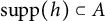

Proof As
 $g^*_A$
is an equilibrium of A, we get
 $\operatorname {\mathrm {supp}}(g^*_A) \subset A$
and thus we have
 . By the monotonicity of the semi-flow, see Lemma 8.5 (1), we have
 for all
 $t \in {\mathbb {R}}_+$
. Then, Proposition 3.1 (3) gives Point (1).
Let A be invariant. For simplicity, we write
 $\phi $
instead of
 $\phi (t, h)$
and
 $\phi '$
for its derivative. By definition of the semi-flow
 $\phi $
, we deduce from (3.2) that

The map
 is thus a solution of Equation (1.2), with F replaced by
 and initial condition
 . By the uniqueness of the semi-flow, we get
 , that is Point (2).
We now assume that
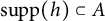 $\operatorname {\mathrm {supp}}(h) \subset A$
. By Point (2), we have
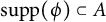 $\operatorname {\mathrm {supp}}( \phi )\subset A$
. We deduce from (3.3) that
 $$\begin{align*}\phi'= F(\phi)=F_A(\phi). \end{align*}$$
Then, the same argument as above yields Point (3).
4 Characterization of equilibria
In this section, we assume that Assumption 2 holds for the SIS model
 $(T, \gamma , \varphi )$
. In particular, the map
 $\varphi $
restricted to
 $[0,1]$
is a decreasing bijection onto
 $[0,1]$
. Recall the operators related to T defined in Section 2.6 and their properties.
4.1 Equilibria, supports, and spectral radius
For any
 $g \in \Delta $
, let
 $L_g$
denote the compact operator on
 $L^p$
defined by
 $$ \begin{align} L_g = M_{\varphi(g)} \, \hat{T}_{1/\gamma}. \end{align} $$
This operator is associated with the linearization
 $M_{\varphi (g)} T - \gamma $
of the dynamics near g in the same way as
 $\hat {T}_{1/\gamma }$
is associated with the linearization
 $T - \gamma $
of the dynamics near
 $0$
(as
 $\varphi (0)=1$
). Notice that when
 $(T, \gamma , \varphi )$
satisfy Assumption 2, then
 $(M_{\varphi (g)} T, \gamma , \varphi )$
also does. It is immediate to check that for
 $g\in \Delta $
:
 $$ \begin{align} g\text{ is an equilibrium} \quad \Longleftrightarrow\quad L_g \, (\gamma g)=\gamma g. \end{align} $$
Lemma 4.1 (Equilibria as nonnegative eigenfunctions)
Let
 $(T, \gamma , \varphi )$
satisfy Assumption 2. Let
 $g\in \Delta $
be an equilibrium. We have the following properties.
-
(1)
$\varphi (g)> 0$
a.e. -
(2) The operators
$ \hat {T}$
,
$\hat {T}_{1/\gamma }$
, and
$L_g$
have the same invariant sets, irreducible sets, atoms, and nonzero atoms. -
(3) The set
$\operatorname {\mathrm {supp}}(g)$
is invariant.


If
 , then the following additional properties hold. Let
 $h\in \Delta $
be an equilibrium. Set
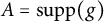 $A= {\operatorname {\mathrm {supp}}(g)}$
.
-
(1)
$\rho (L_g) \geq \rho ((L_g)_A) = 1$
. -
(2) If
$h\leq g$
, then either
$\rho ((L_h)_A) = 1$
and
$h=g$
, or
$\rho ((L_h)_A)>1$
and
$\operatorname {\mathrm {supp}}(h)\neq \operatorname {\mathrm {supp}}(g)$
a.e. -
(3)
$ h\leq g\, \Longleftrightarrow \, \operatorname {\mathrm {supp}}(h) \subset \operatorname {\mathrm {supp}}(g)$
a.e.


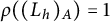

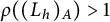


As a consequence of Point (3), we directly get the following corollary.
Corollary 4.2 (Equilibria and their support)
Let
 $(T, \gamma , \varphi )$
that satisfy Assumption 2. Two equilibria with the same support are equal.
Proof of Lemma 4.1
Since
 $\varphi (g) T(g) = \gamma g$
,
 $\varphi (g)$
does not vanish on
 $\operatorname {\mathrm {supp}}(g)$
. On the complement set,
 $g=0$
so
 $\varphi (g)=1$
does not vanish either. Since
 $\varphi $
is nonnegative, we get Point (1).
Point (2) is a direct consequence of the characterization of invariant sets given by (2.8) as
 $1/\gamma $
and
 $\varphi (g)$
are positive by Point (1) and Theorem 2.5 (2) on nonzero atoms. Point (3) is a direct consequence of (4.2), [Reference Delmas, Lefki and Zitt19, Lemma 3.6] (which state that the support of the eigenfunction
 $\gamma g$
is
 $L_g$
-invariant) and Point (2).
Point (1) follows directly from Lemma 2.6 with
 $S=L_g$
,
 $v=\gamma g$
, and
 $\lambda = 1$
.
The proof of Point (2) follows similar lines. Let
 $h\leq g$
be two equilibria with
 . The two eigenvalue equations written for h and g yield
 $ (L_g-L_h) (\gamma g) + L_h(\gamma (g-h)) = \gamma (g-h)$
, which we rewrite as
 $$\begin{align*}L_h (\gamma(g-h)) = \gamma (g-h) + (\varphi(h)-\varphi(g)) Tg. \end{align*}$$
On the right-hand side,
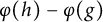 $\varphi (h) - \varphi (g)$
and
 $Tg$
are nonnegative, and by strict monotonicity of
 $\varphi $
they are both positive on
 $B = \operatorname {\mathrm {supp}}(g-h) \subset \operatorname {\mathrm {supp}}(g)$
. If B is empty, then
 $g=h$
and we are back to Point (1). If not, we apply Lemma 2.6 (2) to
 $S = L_h$
,
 $\lambda = 1$
, and
 which is nonnegative:
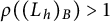 $\rho ((L_h)_B)> 1$
. If B was a subset of
 $\operatorname {\mathrm {supp}}(h)$
this would imply
 $\rho ((L_h)_{\operatorname {\mathrm {supp}}(h)})>1$
, a contradiction with Point (1). So B is not a subset of
 $\operatorname {\mathrm {supp}}(h)$
, or in other words
 $\operatorname {\mathrm {supp}}(h) \neq \operatorname {\mathrm {supp}}(g)$
.
Finally, let us prove Point (3). Clearly,
 $h\leq g$
implies that
 $\operatorname {\mathrm {supp}}(h) \subset \operatorname {\mathrm {supp}}(g)$
. To prove the reverse implication, let us assume that
 $\operatorname {\mathrm {supp}}(h)\subset \operatorname {\mathrm {supp}}(g)$
. Since
 $F( \max (g,h)) \geq 0$
, by Lemmas 8.5 (2) and 8.6, the semi-flow starting from
 $\max (g,h)$
is non-decreasing and converges to an equilibrium
 $\tilde {g}$
, which therefore satisfies
 $\max (g,h) \leq \tilde {g}$
. Since
 $\operatorname {\mathrm {supp}}(\max (g,h)) = \operatorname {\mathrm {supp}}(g)$
is invariant by Point (3), we deduce from Lemma 3.5 (3) that
 $\operatorname {\mathrm {supp}}(\tilde g)\subset \operatorname {\mathrm {supp}}(g)$
and thus
 $\operatorname {\mathrm {supp}}(\tilde {g}) = \operatorname {\mathrm {supp}}(g)$
. Since
 $g\leq \tilde {g}$
, by the previous point, the functions g and
 $\tilde {g}$
must be equal, so
 $g = \max (g,h)$
, or in other words
 $h\leq g$
.
4.2 Maximum equilibria and critical vaccination
Recall the notations of Section 2.6. Let A be a measurable set. Notice the linear map
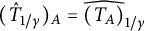 $(\hat {T}_{1/\gamma })_A = \widehat {(T_A)}_{1/\gamma }$
is an operator on
 $L^p$
. Following [Reference Delmas, Dronnier and Zitt17], we then define the basic reproduction number of A as the spectral radius of this operator
 $R_0(A) = \rho ((\hat {T}_{1/\gamma })_A)$
, and simply write
 $R_0$
for
 $R_0(\Omega )$
. Notice that, by (2.5), the map
 $A \mapsto R_0(A)$
is non-decreasing, that is, for any
 $A, B$
measurable sets with
 $A \subset B$
a.e., we have
 $R_0(A) \leq R_0(B)$
.
The following result generalizes [Reference Delmas, Dronnier and Zitt17, Theorems 4.7 and 4.13], and is proved similarly, see Section 9 for details.
Proposition 4.3 Let
 $(T, \gamma , \varphi )$
satisfy Assumption 2. Then, we have the following properties.
-
(1) If
$R_0 \leq 1$
, then we have
, and for all
$h\in \Delta $
: -
(2) If
$R_0> 1$
, then the maximal equilibrium
$g^*$
is non-null, (that is,
$\mu (\operatorname {\mathrm {supp}}(g^*))> 0$
). -
(3) If
$R_0> 1$
and T is quasi-irreducible, that is,
$T = T_A$
with A an irreducible set, then we have
$\operatorname {\mathrm {supp}}(g^*) = A$
a.e. and
$g^*$
is the unique non-null equilibrium. -
(4) If
$R_0> 1$
, T is quasi-irreducible, that is,
$T = T_A$
with A an irreducible set, and
$h\in \Delta $
, then we have
if
$\operatorname {\mathrm {supp}}(h) \cap A=\emptyset $
a.e. and:
$$\begin{align*}\operatorname*{\mbox{lim ess}}_{t\rightarrow +\infty } \phi(t, h)=g^* \quad\text{if}\quad \mu(\operatorname{\mathrm{supp}}(h) \cap A)>0. \end{align*}$$














In the next remarks and examples, we explore the uniformity of the convergence in Point (1) and Proposition 3.1 (3). See also the summarized results from Proposition 5.5.
Remark 4.4 (Exponential rate of convergence to
when
$R_0<1$
and
$\operatorname *{\mbox {ess inf}} \gamma> 0$
)


Assume
 $(T, \gamma , \varphi )$
satisfies Assumption 2,
 $R_0<1$
and
 $\operatorname *{\mbox {ess inf}} \gamma> 0$
. By Lemma 9.2, we also have
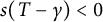 $s(T - \gamma ) < 0$
. Then, mimicking the proof of [Reference Delmas, Dronnier and Zitt17, Theorem 4.6] and using that
 $1-\varphi \geq 0$
, we get that for all
 $c \in (0, -s(T - \gamma ))$
, there exists
 $\theta \in {\mathbb {R}}_+$
such that, for all
 $h \in \Delta $
,
 $t \geq 0$
, we have
 $$\begin{align*}\left\lVert\,\phi(t,h)\,\right\rVert_\infty \leq \theta \left\lVert\,h\,\right\rVert_\infty \, \mathrm{e}^{-ct}. \end{align*}$$
Remark 4.5 (Nonuniform convergence when
$R_0\leq 1$
and
$\operatorname *{\mbox {ess inf}} \gamma =0$
)


We assume that
 $R_0\leq 1$
and
 $\operatorname *{\mbox {ess inf}} \gamma = 0$
. Consider the function v defined by
 $v(t) = \exp (-t\gamma ) \in \Delta $
for
 $t \geq 0$
. As
 $v'(t) - F(v(t))= - \varphi (v(t)) \, T v(t) \leq 0$
, we deduce from Lemma 8.2 and Proposition 7.2 that
 for all
 $t\geq 0$
. We obtain
 as
 $\operatorname *{\mbox {ess inf}} \gamma = 0$
. Thus, the semi-flow
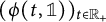 does not converge to
 in
 $L^\infty $
.
Notice the same conclusion holds (with the same arguments) if
 $R_0\leq 1$
is replaced by the more general condition
 $\operatorname *{\mbox {ess sup}} g^*<1$
.
Example 4.6 (A uniform convergence when
$\operatorname *{\mbox {ess inf}} \gamma =0$
)

If
 $\operatorname *{\mbox {ess sup}} g^*=1$
and
 $\operatorname *{\mbox {ess inf}} \gamma = 0$
it is possible for the semi-flow
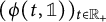
to converge to
 $g^*$
in
 $L^\infty $
. Consider the particular case:
 $\Omega =(0, 1]$
with
 $\mu =\nu + \delta _1$
, where
 $\nu $
is the Lebesgue measure and
 $\delta _1$
the Dirac mass at
 $1$
;

for all
 $f\in L^p$
;
 $\gamma (x)=x/2$
and
 $\varphi (r)=1-r$
. In this case,
 $\{1\}$
is the only atom, and
 $R_0(\{1\})=2$
. We get
 $g^*(x)=1/(1+x)$
and thus
 $\operatorname *{\mbox {ess sup}} g^*=1$
. (Notice that
 $g^*(0+)=\operatorname *{\mbox {ess sup}} g^*$
and
 $\gamma (0+)=\operatorname *{\mbox {ess inf}} \gamma $
.) Elementary calculus give that, for
 $t\geq 0$
,

and for
 $x\in (0, 1)$
:

so that

. So the semi-flow
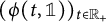
converges to
 $g^*$
in
 $L^\infty $
.
We now focus on critical vaccination. Let
 $\varphi _0$
defined by
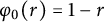 $\varphi _0(r)=1 -r$
and
 $\mathrm {T}_k$
the kernel operator from Remark 1.4 with k and
 $\gamma $
satisfying (1.7) so that
 $(\mathrm {T}_k, \gamma , \varphi _0)$
satisfies Assumption 2. Let
 $\eta \in \Delta $
seen as a perfect vaccination strategy: the SIS model
 $(\mathrm {T}_k M_\eta , \gamma , \varphi _0)$
(which indeed satisfies Assumption 2) corresponds to the initial SIS model, where for
 $x \in \Omega $
, a proportion
 $1-\eta (x)$
of the population is vaccinated and thus does not spread the disease (see [Reference Delmas, Dronnier and Zitt16] and references therein). In this setting, vaccinating the population amounts to replace the measure
 $\mu $
by
 $\eta \mu $
.
Motivated by this example, we shall consider the effective reproduction number defined by
 $$\begin{align*}R_e(\eta) = \rho( \hat{T}_{1/\gamma} M_\eta) , \end{align*}$$
for
 $\eta \in \Delta $
(notice that
 $(TM_\eta , \gamma , \varphi )$
satisfies Assumption 2 and
 $\hat {T}_{1/\gamma } M_\eta =\widehat {(TM_n)}_{1/\gamma }$
). Following [Reference Delmas, Dronnier and Zitt16], we shall be interested in critical vaccination
 $\eta $
for which
 $R_e(\eta ) = 1$
. It is observed in [Reference Delmas, Dronnier and Zitt18] that for the SIS model
 $(\mathrm {T}_k, \gamma , \varphi _0)$
, the vaccination strategy
 $\eta =\varphi _0(g^*)$
is critical. We generalize this result (with a shorter proof based on the fact that
 $R_e(\varphi (g))=\rho (L_g)$
, see (4.1)) for more general operators T and functions
 $\varphi $
.
Theorem 4.7 (Equilibria and critical vaccination)
Let
 $(T, \gamma , \varphi )$
that satisfy Assumption 2. Let
 $h \in \Delta $
be an equilibrium. Then, we have
 $h = g^* \, \Longleftrightarrow \, R_e(\varphi (h)) \leq 1$
. If furthermore
 $R_0> 1$
, then we have
 $$\begin{align*}h = g^* \, \Longleftrightarrow \, R_e(\varphi(h)) = 1. \end{align*}$$
Proof First, remark that
 $\rho (L_g) = R_e(\varphi (g))$
, where
 $L_g$
is defined by (4.1).
If
 $R_0 \leq 1$
, then by Proposition 4.3, we have
 . As
 $R_e(\varphi (0)) = R_0 \leq 1$
by Assumption 2, we directly get the equivalence
 $h = g^* \, \Longleftrightarrow \, R_e(\varphi (h)) \leq 1$
.
If
 $R_0> 1$
, then we have
 by Proposition 4.3. According to Lemma 4.1 (1), if
 , we have
 $R_e(\varphi (h))=\rho (L_h)\geq 1$
, and by (2.5) and (2) that if
 $h\neq g^*$
then
 $\rho (L_h) \geq \rho \big ((L_h)_A\big )>1$
with
 $A={\operatorname {\mathrm {supp}}(g^*)}$
.
To complete the proof, that is,
 $R_e(\varphi (g^*))=1$
, we shall assume that
 $\rho (L_h)>1$
and show that
 $h\neq g^*$
. Informally, the idea is to follow the unstable direction at the equilibrium h to construct a trajectory leading to another equilibrium. Since
 $L_h$
is a positive compact operator, thanks to the Krein–Rutman theorem (Theorem 2.5 (1)), we can consider an eigenvector
 of
 $L_h$
related to
 $\rho (L_h)$
. Since the set
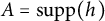 $A=\operatorname {\mathrm {supp}}(h)$
is invariant by Lemma 4.1 (3), we have

If
 was equal to
 ,
 $\rho (L_h)> 1$
would be an eigenvalue of
 $(L_h)_A$
, contradicting Lemma 4.1 (1). As A is invariant and
 , multiplying (4.3) by
 gives
 , showing that
 is an eigenvector of
 $(L_h)_{A^c}$
, so
 $\rho ((L_h)_{A^c})= \rho (L_h)>1$
.
Since
 $(L_h)_{A^c} = M_{\varphi (h)} (\hat {T}_{1/\gamma })_{A^c} = \widehat {(T_{A^c})}_{1/\gamma }$
(as
 $h=0$
on
 $A^c$
and
 $\varphi (0)=1$
), we may apply Proposition 9.3 with
 $T=T_{A^c}$
: there exists a
 $\lambda>0$
and
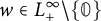 such that
 $T_{A^c} w - \gamma w = \lambda w$
. Without loss of generality, we can assume that
 $\left \lVert \,w\,\right \rVert _\infty $
is small enough to ensure that
 $ w \in \Delta $
and, as
 $\varphi $
is continuous with
 $\varphi (0)=1$
, that
 $\varphi ( \left \lVert \,w\,\right \rVert _\infty ) \geq 1- \delta $
with
 $\delta>0$
small enough so that
 $\delta (\lambda + \left \lVert \,\gamma \,\right \rVert _\infty ) \leq \lambda $
. Note that
 $\operatorname {\mathrm {supp}}(w) \subset A^c$
. Since
 , and
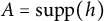 $A=\operatorname {\mathrm {supp}}(h)$
is invariant, we get
 $ \varphi (h+ w) Th = \varphi (h) Th$
. Since h is an equilibrium, we obtain that
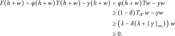 $$ \begin{align*} F(h + w) = \varphi(h+ w) T(h+ w) - \gamma (h+ w) &= \varphi(h+ w) Tw - \gamma w \\ &\geq (1-\delta) T_{A^c}w - \gamma w \\ &\geq \left( \lambda - \delta(\lambda + \left\lVert\,\gamma\,\right\rVert_\infty ) \right) \, w\\ & \geq 0. \end{align*} $$
By Lemmas 8.5 (2) and 8.6, this implies that the trajectory starting from
 $h+ w$
converges monotonously to an equilibrium g. Since
 $h\leq h+ w \leq g\leq g^*$
and
 , we get that
 $h\neq g^*$
as claimed.
4.3 Equilibria and antichains of atoms
We now focus on the characterization of equilibria. We recall from (2.9) that the future of an antichain
 $\mathcal {C}$
of atoms (which is at most countable) is given by
 $ \mathcal {F}(\mathcal {C}) = \mathcal {F} \left ( \bigcup _{A \in \mathcal {C}} A \right )= \bigcup _{A \in \mathcal {C}} \mathcal {F} \left ( A \right )$
. The set of supercritical atoms:
 $$\begin{align*}\mathfrak{A}^{\mathrm{sup}}=\{A\in \mathfrak{A}\, \colon\, R_0(A)>1\} \end{align*}$$
is finite by [Reference Delmas, Lefki and Zitt19, Lemma 6.5]. We say an antichain
 $\mathcal {C}$
of atoms is supercritical if all its elements are supercritical atoms, that is,
 $\mathcal {C}\subset \mathfrak {A}^{\mathrm {sup}}$
. We denote by
 $\mathfrak {S}$
the (finite) set of supercritical antichains. For a set A, let
 $\mathcal {C}_A$
denote the (possibly empty) supercritical antichain given by the maximal elements of
 $\{B \in \mathfrak {A}^{\mathrm {sup}}\, \colon \, B \subset A \text { a.e.}\}$
. Notice that when A is admissible, we get by (2.10) that
 $\mathcal {C}_A$
is non-empty if and only if
 $R_0(A)>1$
. For
 $h\in \Delta $
, we simply write
 $\mathcal {C}_h$
for
 $\mathcal {C}_{\operatorname {\mathrm {supp}}(h)}$
.
The following theorem generalizes the uniqueness result of Proposition 4.3 when the operator T is not necessarily quasi-irreducible. Recall that, by Lemma 4.1 (3), equilibria are characterized by their support.
Theorem 4.8 (Equilibria and supercritical antichains are in bijection)
Let
 $(T, \gamma , \varphi )$
satisfy Assumption 2. The set of the equilibria and the set of supercritical antichains are in bijection through the equivalent relations:
 $$ \begin{align} \operatorname{\mathrm{supp}}(g)= \mathcal{F}(\mathcal{C}) \quad \Longleftrightarrow \quad \mathcal{C}_g= \mathcal{C} , \end{align} $$
where
 $g\in \Delta $
is an equilibrium and
 $\mathcal {C}\in \mathfrak {S}$
a supercritical antichain. Furthermore, if
 , then the equilibrium g is the maximal equilibrium of
 $\mathcal {F}(\mathcal {C}_g)$
.
We divide the proof in two lemmas.
Lemma 4.9 (Support of an equilibrium and related supercritical antichain)
If
 $g \in \Delta $
is an equilibrium, then we have
 $\operatorname {\mathrm {supp}}(g) = \mathcal {F}\left (\mathcal {C}_g\right )$
a.e. In particular, if g and h are two equilibria, we get
 $$\begin{align*}\mathcal{C}_g=\mathcal{C}_h \Longleftrightarrow g=h. \end{align*}$$
Proof As the set
 $\operatorname {\mathrm {supp}}(g)$
is invariant by Lemma 4.1 (3) and as every element of
 $\mathcal {C}_g$
is included in
 $\operatorname {\mathrm {supp}}(g)$
, we have
 $\mathcal {F}(\mathcal {C}_g) \subset \operatorname {\mathrm {supp}}(g)$
.
By construction of
 $\mathcal {C}_g$
, every atom
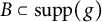 $B\subset \operatorname {\mathrm {supp}}(g)$
with
 $R_0(B)>1$
is included in
 $\mathcal {F}(\mathcal {C}_g)$
. This implies by (2.10) that, with
 $A=\operatorname {\mathrm {supp}}(g) \cap \mathcal {F}(\mathcal {C}_g)^c$
an invariant (by Lemma 4.1 (3)) and thus admissible set:
 $$\begin{align*}R_0(A) = \max_{ B\subset A, \, B\in \mathfrak{A}} R_0(B) \leq 1. \end{align*}$$
Then Lemma 3.4 (3) gives that
 is an equilibrium of
 $\mathcal {F}(\mathcal {C}_g)^c$
and of A. Then, Proposition 4.3 (1) (with the SIS model
 $(T_A, \gamma , \varphi )$
) implies that
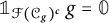 , that is,
 $\operatorname {\mathrm {supp}}(g) \subset \mathcal {F}(\mathcal {C}_g)$
. Thus, we get
 $\operatorname {\mathrm {supp}}(g)=\mathcal {F}(\mathcal {C}_g) $
. The second part of the lemma is then a direct consequence of Corollary 4.2 and Lemma 2.1.
Lemma 4.10 For any supercritical antichain
 $\mathcal {C}$
, there exists an equilibrium
 $g\in \Delta $
such that
 $\mathcal {C} = \mathcal {C}_g$
. If
 $\mathcal {C}$
is nonempty, then
 is the maximal equilibrium of
 $\mathcal {F}(\mathcal {C})$
.
Proof If
 $\mathcal {C}$
is empty, then taking the equilibrium
 , we get
 $\mathcal {C}=\mathcal {C}_g$
. We assume now that
 $\mathcal {C}$
is not empty. Let g be the maximal equilibrium on
 $\mathcal {F}(\mathcal {C})$
. It is also an equilibrium by Lemma 3.4 (2) and
 $\operatorname {\mathrm {supp}}(g)\subset \mathcal {F}(\mathcal {C})$
. For any
 $A\in \mathcal {C}$
, we have
 $g^*_A \leq g$
by Lemma 3.3, and
 $g^*_A$
is positive on A by Proposition 4.3 (3) since A is a supercritical atom and thus an irreducible set with
 $R_0(A)>1$
. This implies that
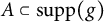 $A\subset \operatorname {\mathrm {supp}}(g)$
and thus
 $\mathcal {F}(A) \subset \operatorname {\mathrm {supp}}(g)$
as
 $\operatorname {\mathrm {supp}}(g)$
is invariant. Then use (2.9) to get
 $\mathcal {F}(\mathcal {C}) \subset \operatorname {\mathrm {supp}}(g)$
, so that
 $\mathcal {F}(\mathcal {C})=\operatorname {\mathrm {supp}}(g)$
, and thus
 $\mathcal {F}(\mathcal {C})=\mathcal {F}(\mathcal {C}_g)$
by Lemma 4.9. The two antichains
 $\mathcal {C}$
and
 $\mathcal {C}_g$
have the same future and are thus equal by Lemma 2.1. The proof is then complete.
Let
 $\mathcal {E}\subset \Delta $
denote the set of equilibria of the SIS model
 $(T, \gamma , \varphi )$
.


4.4 Monatomicity and order relation via equilibria
Let
 $(T, \gamma , \varphi )$
that satisfy Assumption 2. Consider the SIS model
 $(T, \lambda \gamma , \varphi )$
with recovery rate
 $ \gamma $
multiplied by a real parameter
 $\lambda>0$
. The reproduction number of a measurable set A for this model is
 $\rho ((\hat {T}_{1/\lambda \gamma })_A)= \rho ((\hat {T}_{1/ \gamma })_A\, M_{1/\lambda } )=R_0(A)/\lambda $
. We deduce from Theorem 4.8 that the number of equilibria of the SIS model
 $(T, \lambda \gamma , \varphi )$
is decreasing with
 $\lambda $
.
We say that the operator T on
 $L^p$
for
 $p \in (1, +\infty )$
is monatomic if it has exactly one nonzero atom, that is,
 $\operatorname {\mathrm {card}}(\mathfrak {A}^*) = 1$
. Monatomicity is a natural extension of (quasi-)irreducibility (see [Reference Delmas, Lefki and Zitt19, Remark 1.2] and references therein). We complete the characterization of monatomic operator T given in [Reference Delmas, Lefki and Zitt19, Theorem 2] using the number of equilibria of the SIS models
 $(T, \lambda \gamma , \varphi )$
.
Corollary 4.11 (Criterium of monatomicity)
Let
 $(T, \gamma , \varphi )$
satisfy Assumption 2. The operator T is monatomic if and only if the two following properties hold:
-
(1) For
$\lambda> 0$
, the SIS model
$(T, \lambda \gamma , \varphi )$
has at most one non-null equilibrium. -
(2) There exists
$\lambda> 0$
such that the SIS model
$(T, \lambda \gamma , \varphi )$
has a non-null equilibrium.


Proof By Theorem 4.8, we deduce that if
 $\mathcal {C}$
is a finite antichain of nonzero atoms then, for all
 $\lambda \in (0, \min _{A\in \mathcal {C}} R_0(A))$
there exists an equilibrium
 $g^\lambda $
for the model
 $(T, \lambda \gamma , \varphi )$
such that
 $\mathcal {F}(\mathcal {C})=\operatorname {\mathrm {supp}}(g^\lambda )$
.
Then, Point (1) means that the number of finite antichains of nonzero atoms is at most two, and Point (2) that it is at least two: so the two points are equivalent to the number of antichains being exactly two (one being empty), that is, T is monatomic.
5 Convergence and attraction domains
In this section, we are interested in the behavior of the semi-flow
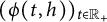 $(\phi (t, h))_{t\in {\mathbb {R}}_+}$
of Equation (1.2) when t goes to infinity for an initial condition
 $h \in \Delta $
. See the summarized results from Proposition 5.5. If T is a quasi-irreducible kernel positive operator, then according to Proposition 4.3 (4), see also [Reference Delmas, Dronnier and Zitt17, Theorem 4.13] when T is an irreducible kernel operator, the semi-flow
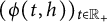 $(\phi (t, h))_{t\in {\mathbb {R}}_+}$
converges essentially to
 $g^*$
if
 $\mu (\operatorname {\mathrm {supp}}(h) \cap \operatorname {\mathrm {supp}}(g^*))> 0$
and
 otherwise. We generalize this result to general operators, see Section 10 for a proof.
Theorem 5.1 (Convergence to an equilibrium)
Let
 $(T, \gamma , \varphi )$
satisfy Assumption 2. The semi-flow
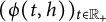 $(\phi (t, h))_{t\in {\mathbb {R}}_+}$
with initial condition
 $h\in \Delta $
converges essentially to a limit, say
 $g\in \Delta $
; and g is an equilibrium and more precisely the maximal equilibrium of the set
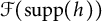 $\mathcal {F}(\operatorname {\mathrm {supp}}(h))$
:
 $$\begin{align*}\operatorname*{\mbox{lim ess}}_{t\rightarrow \infty } \phi(t, h) = g \quad\text{and}\quad \mathcal{C}_g=\mathcal{C}_{\mathcal{F}(\operatorname{\mathrm{supp}}(h))}. \end{align*}$$
We derive directly the next corollary, where the maximal equilibrium
 $g^*$
is possibly equal to
 .
Corollary 5.2 (Attraction domain of the maximum equilibrium)
Let
 $(T, \gamma , \varphi )$
satisfy Assumption 2. The semi-flow with initial condition
 $h\in \Delta $
converges essentially to the maximal equilibrium
 $g^*$
, that is,
 $\operatorname *{\mbox {lim ess}}_{t\rightarrow \infty } \phi (t, h) = g^*$
, if and only if
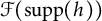 $\mathcal {F}(\operatorname {\mathrm {supp}}(h))$
contains all the supercritical atoms.
In particular, we recover Proposition 4.3 as
 $R_0\leq 1$
means there is no supercritical atom, and
 $R_0>1$
and T quasi-irreducible means there is only one supercritical atom. In the previous corollary, it may however happen that none of the supercritical atoms is included in
 $\operatorname {\mathrm {supp}}(h)$
, see the next example.
Example 5.3 Let
 $\Omega = \{a,b\}$
with the counting measure, and consider the SIS model
 $(T, \gamma , \varphi )$
with T identified with the matrix
 $\begin {pmatrix} 1 & 0 \\ \star & 2 \end {pmatrix}$
(with
 $\star> 0$
),
 ,
 $\varphi (r) = 1-r$
. Notice that
 $\{a\}$
and
 $\{b\}$
are nonzero atoms, the former being critical with
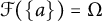 $\mathcal {F}(\{a\})=\Omega $
and the latter being supercritical and invariant. Thus, there exists only two equilibria:
 and
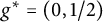 $g^*=(0,1/2)$
. If
 , then we have
 $\lim _{t\rightarrow \infty } \phi (t, h) = g^*$
. For
 $h=(0,1)$
, we have
 $\operatorname {\mathrm {supp}}(h)=\operatorname {\mathrm {supp}}(g^*)$
, but for
 $h = (1,0)$
we have
 $\operatorname {\mathrm {supp}}(h) \cap \operatorname {\mathrm {supp}}(g^*) =~\emptyset $
.
Proposition 5.4 (Uniform convergence to an equilibrium)
Let
 $(T, \gamma , \varphi )$
satisfy Assumption 2. For
 $h \in \Delta $
and g, the maximal equilibrium of
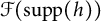 $\mathcal {F}(\operatorname {\mathrm {supp}}(h))$
, we have that
 $$ \begin{align} \lim_{t\rightarrow \infty } \left\lVert\,\big(\phi(t,h)-g\big)\, \gamma \,\right\rVert_\infty =0. \end{align} $$
In particular, when
 $\operatorname *{\mbox {ess inf}} \gamma> 0$
, the convergence given by Theorem 5.1 is uniform. Notice we have a stronger result if furthermore
 $R_0<1$
(and thus
 ) (see Remark 4.4).
Proof We start with a preliminary result. Set M as the norm of the operator
 ${\tilde {T}} $
from
 $L^p$
to
 $L^\infty $
, which coincide with T on
 $L^\infty $
, see the proof of Lemma 2.8; it is finite by Assumption 2. Let
 $m>0$
. Let
 $h_1\geq h_2$
be elements of
 $\Delta $
, and for
 $t\in {\mathbb {R}}_+$
set
 $f(t) = \phi (t, h_1) - \phi (t, h_2)$
. We claim that

Indeed, by monotonicity of the semi-flow (see Lemma 8.5), we have
 $\phi (t, h_1) \geq \phi (t, h_2)$
and thus

. We also have, as
 $\varphi $
is decreasing on
 $[0,1]$
and T is positive that for
 $t\in {\mathbb {R}}_+$
:
 $$ \begin{align*} f'(t) &= \varphi(\phi(t, h_1)) T\phi(t, h_1) - \varphi(\phi(t, h_2)) T\phi(t, h_2) - \gamma f(t)\\ &\leq \varphi(\phi(t, h_1)) Tf(t) - \gamma f(t)\\ &\leq Tf(t) - \gamma f(t). \end{align*} $$
On
 $\{\gamma \geq m\}$
, we get for
 $v(t)=\mathrm {e}^{mt} f(t)$
that for all
 $t \geq 0$
:
 $$ \begin{align} v'(t) \leq (m - \gamma) v(t) + T v(t) \leq \left\lVert\,{\tilde{T}} \, \iota v(t)\,\right\rVert_\infty \leq M \left\lVert\,v(t)\,\right\rVert_p. \end{align} $$
By (7.1) and (7.2) on the Bochner integral, we deduce that
 $v(t) \leq v(0) + M \int _0^t \left \lVert \,v(s)\,\right \rVert _p\, \mathrm {d} s$
on
 $\{\gamma \geq m\}$
. Since f is nonnegative, we get

This gives (5.2).
Let
 $h \in \Delta $
and g be the maximal equilibrium of
 $A=\mathcal {F}(\operatorname {\mathrm {supp}}(h))$
. By Lemma 9.1, we have
 $\operatorname {\mathrm {supp}}(\phi (1,h)) = A$
. Let
 $h_1 = \max (\phi (1,h), g)$
and
 $h_2 = \min (\phi (1,h), g)$
. We thus have
 $h_1\leq h_2$
and
 $\operatorname {\mathrm {supp}}(g)=\operatorname {\mathrm {supp}}(h_2)\subset \operatorname {\mathrm {supp}}(h_1)=A$
. By Theorem 5.1 (and using that g is the maximal equilibrium on the invariant set
 $\mathcal {F}(\operatorname {\mathrm {supp}}(h_i))$
for
 $i=1, 2$
), we get that
 $\operatorname *{\mbox {lim ess}}_{t\rightarrow \infty } \phi (t, h_i)=g$
for
 $i=1, 2$
. With
 $f(t) = \phi (t, h_1) - \phi (t, h_2)$
, we get by the dominated convergence theorem that
 $\lim _{t\rightarrow \infty } \left \lVert \,f(t)\,\right \rVert _p=0$
, and by (5.2) that
 for all
 $m>0$
and thus
 $\lim _{t\rightarrow \infty } \left \lVert \, f(t)\, \gamma \,\right \rVert _\infty =0$
as
 $\left \lVert \,f\,\right \rVert _\infty \leq 1$
. Use the monotonicity of the semi-flow to get
 $\phi (t, h_1) \geq \phi (t+1, h) \geq \phi (t, h_2)$
and deduce that (5.1) holds.
We summarize the convergence results assuming in the last two cases that
 $\gamma $
is bounded away from
 $0$
to simplify (see Theorem 5.1, Proposition 5.4, and Remark 4.4).
Proposition 5.5 (Convergence to an equilibrium)
Let
 $(T, \gamma , \varphi )$
satisfy Assumption 2. For
 $h \in \Delta $
and g the maximal equilibrium of
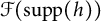 $\mathcal {F}(\operatorname {\mathrm {supp}}(h))$
:
-
(1) We have
$\operatorname *{\mbox {lim ess}}_{t\rightarrow \infty } \phi (t, h) = g$
. -
(2) When
$\operatorname *{\mbox {ess inf}} \gamma> 0$
, we have the uniform convergence
$\lim _{t\rightarrow \infty } \left \lVert \, \phi (t,h)-g\,\right \rVert _\infty =0. $
-
(3) When
$\operatorname *{\mbox {ess inf}} \gamma> 0$
and
$R_0 < 1$
, the convergence to
is at exponential rate that does not depend on the initial condition, that is, for all
$c \in (0, -s(T - \gamma ))$
, there exists
$\theta \in {\mathbb {R}}_+$
such that, for all
$h' \in \Delta $
,
$t \geq 0$
, we have
$$\begin{align*}\left\lVert\,\phi(t,h')\,\right\rVert_\infty \leq \theta \left\lVert\,h'\,\right\rVert_\infty \, \mathrm{e}^{-ct}. \end{align*}$$









6 SIS model with an external disease reservoir
In this section, we consider the infinite-dimensional inhomogeneous SIS model with an external disease reservoir, called SIS
 $\kappa $
model, presented in Section 1.4. The function
 $u=(u(t,x))_{t\in {\mathbb {R}}_+, x\in \Omega }$
, where
 $u(t,x)$
is the proportion of infected population among the population with feature x, is solution in
 $L^\infty $
of the ODE:
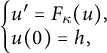 $$ \begin{align} \left\{\begin{array}{@{}l} u' = F_\kappa(u), \\ u(0) = h, \end{array}\right. \end{align} $$
with initial condition
 $h\in L^\infty $
and:
 $$ \begin{align} F_\kappa(u)= \varphi(u) (Tu+\kappa) - \gamma u, \end{align} $$
where
 $\varphi $
is a continuous function on
 ${\mathbb {R}}$
and
 $\kappa \in L^\infty _+$
. To study solutions of (6.1) and the corresponding equilibria, that is functions
 $g \in \Delta $
such that
 $F_\kappa (g) = 0$
, we shall use the formalism of Section 3 by adding a sub-population corresponding to the reservoir with type
 ${\mathbf {r}}$
. Notice the case
 $\varphi ([0, 1])=\{0\}$
(which is not possible under Assumption 2) is trivial, and thus we shall assume there exists
 $a\in (0, 1)$
such that
 $\varphi (a)>0$
.
We set
 $\Omega _{\mathbf {r}}=\Omega \sqcup \{{\mathbf {r}}\}$
(assuming without loss of generality that
 ${\mathbf {r}}\not \in \Omega $
),
 $\mathcal {G}_{\mathbf {r}} = \sigma (\mathcal {G}, \{{\mathbf {r}}\})$
and
 $\mu _{\mathbf {r}}$
a measure on
 $(\Omega _{\mathbf {r}}, \mathcal {G}_{\mathbf {r}})$
which coincides with
 $\mu $
on
 $\Omega $
and with positive finite weight on
 ${\mathbf {r}}$
. For a function
 $f_{\mathbf {r}}$
defined on
 $\Omega _{\mathbf {r}}$
, we simply write f for its restriction to
 $\Omega $
(and similarly, for a function f defined on
 $\Omega $
, we write
 $f_{\mathbf {r}}$
for a function defined on
 $\Omega _{\mathbf {r}}$
which coincides with f on
 $\Omega $
, the value of
 $f_{\mathbf {r}}$
on
 ${\mathbf {r}}$
being given when needed). We simply write
 $L^p_{\mathbf {r}}$
for
 $L^p(\Omega _{\mathbf {r}}, \mathcal {G}_{\mathbf {r}}, \mu _{\mathbf {r}})$
, where
 $p\in [1, +\infty ]$
. We define the positive operator
 $T_{\mathbf {r}}$
on
 $L^\infty _{\mathbf {r}}$
, as an extension of T on
 $\Omega _{\mathbf {r}}$
, by

with
 $\alpha _{\mathbf {r}}\in (L^\infty _{\mathbf {r}}) _+$
such that
 $\alpha =\kappa /a$
on
 $\Omega $
, with
 $a\in (0, 1)$
, and
 $\alpha _{\mathbf {r}}({\mathbf {r}})=b>0$
. For
 $p \in (1,+\infty )$
, we define similarly the operator
 $\hat {T}_{\mathbf {r}}$
on
 $L^p_{\mathbf {r}}$
based on the operator
 $\hat {T}$
on
 $L^p$
(see Lemma 2.8). We also define the function
 $\gamma _{\mathbf {r}}$
(which coincides with
 $\gamma $
on
 $\Omega $
by definition) such that
 $\gamma _{\mathbf {r}}({\mathbf {r}})= b\varphi (a) $
is assumed to be positive (that is,
 $\varphi (a)>0$
). Let
 $\Delta _{\mathbf {r}}=\{f_{\mathbf {r}}\in (L^\infty _{\mathbf {r}})_+\, \colon \, 1-f_{\mathbf {r}} \in (L^\infty _{\mathbf {r}})_+\}$
be the analog of
 $\Delta $
for
 $\Omega _{\mathbf {r}}$
. It is elementary to check the following result.
Proposition 6.1 (Solution to the SIS
$\kappa $
model)

Let
 $(T, \gamma , \varphi )$
satisfy Assumption 1. Assume furthermore there exists
 $a\in (0, 1)$
such that
 $\varphi (a)>0$
, and let
 $\kappa \in L_+^\infty $
. A function
 $(u(t, x))_{t\in {\mathbb {R}}_+, x\in \Omega }$
is a solution to (6.1) related to the SIS
 $\kappa $
model with initial condition
 $h\in \Delta $
if and only if the function
 $(u_{\mathbf {r}}(t, x))_{t\in {\mathbb {R}}_+, x\in \Omega _{\mathbf {r}}}$
, where
 $u_{\mathbf {r}}(t, {\mathbf {r}})=a$
for all
 $t\in {\mathbb {R}}_+$
, is a solution to (1.2) related to the SIS model with parameter
 $(T_{\mathbf {r}}, \gamma _{\mathbf {r}}, \varphi )$
on
 $\Omega _{\mathbf {r}}$
and with initial condition
 $h_{\mathbf {r}}\in \Delta _{\mathbf {r}}$
such that
 $h_{\mathbf {r}}({\mathbf {r}})=a$
.
We shall consider the supercritical atoms out of the individuals infected by the reservoir:
 $$\begin{align*}\mathfrak{A}^{\mathrm{sup}}_{\mathbf{r}}=\{A \in \mathfrak{A}^{\mathrm{sup}}\, \colon\, A\cap \mathcal{F}(\operatorname{\mathrm{supp}}(\kappa))=\emptyset \text{ a.e.}\}. \end{align*}$$
Based on Theorems 4.8 and 5.1 for the
 $(T_{\mathbf {r}}, \gamma _{\mathbf {r}}, \varphi )$
SIS model we can give a representation of the equilibria of SIS
 $\kappa $
model, that is, of the solutions to
 $F_\kappa (g)=0$
in
 $\Delta $
, prove that the equilibria are characterized by their support, and explicit their attraction domain. For a function
 $h\in L^\infty _+$
, we shall denote
 $\mathcal {C}_{{\mathbf {r}}, h}$
the antichain given by the maximal elements of
 $\{B \in \mathfrak {A}^{\mathrm {sup}}_{\mathbf {r}}\, \colon \, B \subset \mathcal {F}(\operatorname {\mathrm {supp}}(h)) \text { a.e.}\}$
. Notice that Assumption 2 implies that
 $\varphi $
is positive on
 $[0, 1)$
.
Corollary 6.2 (Equilibria of the SIS
$\kappa $
model)

Let
 $(T, \gamma , \varphi )$
satisfy Assumption 2 and
 $\kappa \in L_+^\infty $
. The set of equilibria and the set of antichains in
 $\mathfrak {A}^{\mathrm {sup}}_{\mathbf {r}}$
are in bijection through the equivalent relations:
 $$\begin{align*}\operatorname{\mathrm{supp}}(g) = \mathcal{F}(\mathcal{C})\cup \mathcal{F}(\operatorname{\mathrm{supp}}(\kappa)) \quad\text{a.e.} \quad \Longleftrightarrow \quad \mathcal{C}_{{\mathbf{r}},g} =\mathcal{C}, \end{align*}$$
where
 $\mathcal {C}\subset \mathfrak {A}^{\mathrm {sup}}_{\mathbf {r}}$
is an antichain and
 $g\in \Delta $
an equilibrium, that is,
 $F_\kappa (g)=0$
.
Furthermore, the semi-flow
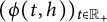 $(\phi (t, h))_{t\in {\mathbb {R}}_+}$
solution of (6.1) with initial condition
 $h\in \Delta $
is well defined and it converges a.e. to a limit, say
 $g\in \Delta $
; and g is an equilibrium and more precisely:
 $$\begin{align*}\operatorname*{\mbox{lim ess}}_{t\rightarrow \infty } \phi(t, h) = g \quad\text{and}\quad \mathcal{C}_{{\mathbf{r}},g}=\mathcal{C}_{{\mathbf{r}}, h}. \end{align*}$$
Remark 6.3 We deduce the following properties under the hypothesis of Corollary 6.2.
-
(1) Notice that
$\mathfrak {A}^{\mathrm {sup}}_{\mathbf {r}}$
is empty if and only if there exists a unique equilibrium
$g\in \Delta $
for the SIS
$\kappa $
model. In this case, we have
$\operatorname {\mathrm {supp}}(g) = \mathcal {F}(\operatorname {\mathrm {supp}}(\kappa ))$
a.e. and
$\operatorname *{\mbox {lim ess}}_{t\rightarrow \infty } \phi (t, h) = g$
for all
$h\in \Delta $
. -
(2) If
$\operatorname *{\mbox {ess inf}} \kappa>0$
, then
$\mathfrak {A}^{\mathrm {sup}}_{\mathbf {r}}$
is empty. -
(3) If g is an equilibrium for the SIS
$\kappa $
model, then g is positive on
$\mathcal {F}(\operatorname {\mathrm {supp}}(\kappa ))$
and thus on
$\operatorname {\mathrm {supp}}(\kappa )$
.






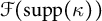

Proof of Corollary 6.2
If
 $A\in \mathcal {G}$
is invariant for
 $\hat {T}$
, then A seen as an element of
 $\mathcal {G}_{\mathbf {r}}$
is also invariant for
 $\hat {T}_{\mathbf {r}}$
. Furthermore, the reservoir
 $\{{\mathbf {r}}\}$
is an atom of
 $\mu _{\mathbf {r}}$
and, as
 $\Omega $
is
 $\hat {T}_{\mathbf {r}}$
-invariant, we get that
 $\{{\mathbf {r}}\}$
is a
 $\hat {T}_{\mathbf {r}}$
-atom. We deduce that a set
 $B\in \mathcal {G}_{\mathbf {r}}$
is admissible for
 $\hat {T}_{\mathbf {r}}$
if and only if
 $B \cap \Omega $
is admissible for
 $\hat {T}$
. In particular a set A is an atom of
 $\hat {T}_{\mathbf {r}}$
if and only if either
 $A=\{{\mathbf {r}}\}$
or
 $A \subset \Omega $
and A is an atom of
 $\hat {T}$
. We denote by
 $\mathcal {F}_{\mathbf {r}}(A)$
the future of a set
 $A\subset \Omega _{\mathbf {r}}$
with respect to
 $\hat {T}_{\mathbf {r}}$
. Notice that
 $\mathcal {F}_{\mathbf {r}}(A)=\mathcal {F}(A)$
for any
 $ A\subset \Omega $
and that the future of the reservoir is
 $$ \begin{align} \mathcal{F}_{\mathbf{r}}(\{{\mathbf{r}}\})=\{{\mathbf{r}}\} \cup \mathcal{F}(\operatorname{\mathrm{supp}}(\kappa)). \end{align} $$
Recall the basic reproduction number
 $R_0(A)$
of a measurable set for the SIS model
 $(T, \gamma , \varphi )$
given in Section 4.2. We simply write
 $R_{\mathbf {r}}(A)$
when considering the basic reproduction number of
 $A \in \mathcal {G}_{\mathbf {r}}$
for the SIS model
 $(T_{\mathbf {r}}, \gamma _{\mathbf {r}}, \varphi )$
. Since
 $(T_{\mathbf {r}})_A=T_A$
for
 $A\subset \Omega $
measurable, we deduce that
 $R_{\mathbf {r}}(A)=R_0(A)$
for any
 $ A\subset \Omega $
measurable. We also have
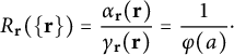 $$\begin{align*}R_{\mathbf{r}}(\{{\mathbf{r}}\})=\frac{\alpha_{\mathbf{r}}({\mathbf{r}})}{\gamma_{\mathbf{r}}({\mathbf{r}})}=\frac{1}{\varphi(a)}\cdot \end{align*}$$
Note that under Assumption 2, we have
 $\varphi ((0, 1))=(0, 1)$
and thus the atom
 $\{{\mathbf {r}}\}$
is super-critical for the
 $(T_{\mathbf {r}}, \gamma _{\mathbf {r}}, \varphi )$
SIS model.
We deduce from Proposition 6.1. that a function
 $g\in \Delta $
is an equilibrium for the SIS
 $\kappa $
model if and only if
 $g_{\mathbf {r}}\in \Delta _{\mathbf {r}}$
, such that
 $g_{\mathbf {r}}({\mathbf {r}})>0$
is an equilibrium for the
 $(T_{\mathbf {r}}, \gamma _{\mathbf {r}}, \varphi )$
SIS model on
 $\Omega _{\mathbf {r}}$
. Notice that necessarily
 $g_{\mathbf {r}}({\mathbf {r}})=a$
. The equilibria of the
 $(T_{\mathbf {r}}, \gamma _{\mathbf {r}}, \varphi )$
SIS model whose support contains the reservoir
 $\{{\mathbf {r}}\}$
are according to Theorem 4.8 in bijection will all the supercritical antichains containing the atom
 $\{{\mathbf {r}}\}$
. Those supercritical antichains are exactly the antichains of
 $\mathfrak {A}^{\mathrm {sup}}_{\mathbf {r}}$
with the atom
 $\{{\mathbf {r}}\}$
added to them. Then, use (6.3) and Theorems 4.8 and 5.1 to conclude.
7 A short reminder on integration, derivation, and ODE in Banach space
This section is devoted to the definition and properties of the Bochner integral, the differentiation and differential equations in Banach spaces. We consider
 $(X, \left \lVert \,\cdot \,\right \rVert )$
a real Banach space.
7.1 Integration in Banach spaces
We give a short summary on the Bochner integral, and refer to [Reference Arendt, Batty, Hieber and Neubrander4, Reference Seifert, Trostorff and Waurick51] for a more detailed presentation. We consider the Borel
 $\sigma $
-field on
 ${\mathbb {R}}$
and write
 $\nu (\mathrm {d} t)=\mathrm {d} t$
for the Lebesgue measure. Let I be an interval of
 ${\mathbb {R}}$
. A function
 $f\, \colon \, I \mapsto X$
is simple if
 where
 $n\in {\mathbb {N}}$
, the
 $a_k$
’s belong to X and the
 $A_k$
’s are Borel subsets of I with finite Lebesgue measure. We define its Bochner integral as
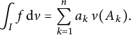 $$\begin{align*}\int _I f\, \mathrm{d} \nu = \sum_{k=1}^n a_k \, \nu(A_k). \end{align*}$$
Notice the integral belongs to X and does not depend on the representation of the simple function f. A function
 $f\, \colon \, I \mapsto X$
is Bochner measurable (simply called measurable in [Reference Arendt, Batty, Hieber and Neubrander4]) if there exists a sequence of simple functions
 $(f_n)_{n\in {\mathbb {N}}}$
, with
 $f_n\, \colon \, I \mapsto X$
, such that
 $\nu $
-a.e.
 $\lim _{n\rightarrow \infty } f_n =f$
(that is,
 $\lim _{n \rightarrow \infty } \left \lVert \,f(t) -f_n(t)\,\right \rVert =0 \mathrm {d} t$
-a.e. on
 $ I$
); it is furthermore Bochner integrable if one can find such approximating sequence
 $(f_n)_{n\in {\mathbb {N}}}$
so that
 $\lim _{n \rightarrow \infty } \int _I \left \lVert \,f(t) - f_n(t)\,\right \rVert \, \mathrm {d} t=0$
. In this case, the Bochner integral of f is defined as
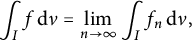 $$\begin{align*}\int _I f\, \mathrm{d} \nu = \lim_{n\rightarrow \infty } \int _I f_n\, \mathrm{d} \nu , \end{align*}$$
where the limit holds in the Banach space. The Bochner integrable
 $ \int _I f\, \mathrm {d} \nu $
does not depend on the approximating sequence
 $(f_n)_{n\in {\mathbb {N}}}$
; we shall also denote it by
 $\int _I f(t)\, \mathrm {d} t$
. Thanks to [Reference Arendt, Batty, Hieber and Neubrander4, Corollary 1.1.2] X-valued continuous function are Bochner measurable and a.e. limits of Bochner measurable function are Bochner measurable. According to [Reference Arendt, Batty, Hieber and Neubrander4, Corollary 1.1.2], a function
 $f\, \colon \, I \mapsto X$
is Bochner integrable if and only if it is Bochner measurable and
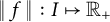 $\left \lVert \,f\,\right \rVert \, \colon \, I \mapsto {\mathbb {R}}_+$
is integrable; in this case, we have
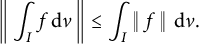 $$ \begin{align} \left\lVert\,\int _I f\, \mathrm{d} \nu\,\right\rVert\leq \int _I \left\lVert\,f\,\right\rVert\, \mathrm{d} \nu. \end{align} $$
When
 $\bar I=[a,b]$
with
 $-\infty \leq a<b\leq +\infty $
and f is Bochner integrable on I, we simply write the Bochner integral as
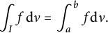 $$\begin{align*}\int _I f \, \mathrm{d} \nu=\int_a^b f \mathrm{d} \nu. \end{align*}$$
The Bochner integral enjoy many properties as the usual Lebesgue integral, as such we shall use the dominated convergence, see [Reference Arendt, Batty, Hieber and Neubrander4, Theorem 1.1.8], which we recall.
Theorem 7.1 (Dominated convergence theorem)
Let I be a non-empty interval of
 ${\mathbb {R}}$
. Let
 $(f_n)_{n \in {\mathbb {N}}}$
be a sequence of Bochner-integrable functions defined on I which converges
 $\nu $
-a.e. to
 $f\, \colon \, I \rightarrow X$
. Assume there exists a Lebesgue-integrable function
 $g \, \colon \, I \rightarrow {\mathbb {R}}_+$
such that
 $\left \lVert \,f_n\,\right \rVert \leq g \nu $
-a.e. for all
 $n \in {\mathbb {N}}$
. Then, the function f is Bochner-integrable and
 $$\begin{align*}\int_I f \, \mathrm{d} \nu = \lim_{n\rightarrow \infty } \int_I f_n\, \mathrm{d} \nu \quad\text{in } X. \end{align*}$$
7.2 Differential equations in Banach spaces
We now consider the derivation of functions on a Banach space. Let I be an interval of
 ${\mathbb {R}}$
with non-empty interior. We say that a function
 $f \, \colon \, I \mapsto X$
is differentiable at a point
 $t \in I$
if the following limit,
 $f'(t)$
, exists in
 $(X, \left \lVert \,\cdot \,\right \rVert )$
:
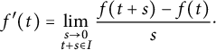 $$\begin{align*}f'(t)= \lim_{\substack{s \rightarrow 0\\t+s\in I}} \frac{f(t+s) - f(t)}{s}\cdot \end{align*}$$
Notice that if f is differentiable at t, then it is continuous at t. We say that f is differentiable on I if it is differentiable at any point of I, and that f belongs to
 $\mathcal {C}^1(I)$
if it is differentiable on I and
 $f'$
is continuous on I. We have the following fundamental theorem of calculus (see [Reference Arendt, Batty, Hieber and Neubrander4, Proposition 1.2.2] and [Reference Seifert, Trostorff and Waurick51, Corollary 3.1.7]). Assume
 $I=[a,b]$
with
 $-\infty <a<b<+\infty $
and that
 $f\, \colon \, I \rightarrow X$
belongs to
 $\mathcal {C}^1(I)$
, then
 $f'$
is Bochner-integrable on I and we have
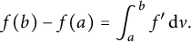 $$ \begin{align} f(b) -f(a)= \int_a^b f'\, \mathrm{d} \nu. \end{align} $$
We now recall some results on differential equations in Banach spaces. Let
 $F\, \colon \, X \rightarrow X$
be locally-Lipschitz, that is, for all
 $x \in X$
, there exists
 $\eta> 0$
and
 $ C$
finite such that for all
 $y \in X$
, we have
 $$\begin{align*}\left\lVert\,x-y\,\right\rVert \leq \eta\quad \Longrightarrow \quad \left\lVert\,F(x) - F(y)\,\right\rVert \leq C \left\lVert\,x-y\,\right\rVert. \end{align*}$$
The Picard–Lindelöf theorem, see [Reference Lang33, Corollaries IV 1.6-8], ensures the existence of
 $(u,\tau )$
, with
 $\tau \in (0, +\infty ]$
and
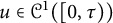 $u\in \mathcal {C}^1([0, \tau ))$
taking values in X, that is a solution to the Cauchy problem:
 $$ \begin{align} \left\{\begin{array}{@{}l} u' = F(u), \\ u(0) = x, \end{array}\right. \end{align} $$
where the first equality in (7.3) holds in
 $[0, \tau )$
and
 $x\in X$
is the so-called initial condition, and furthermore the solution
 $(u,\tau )$
is unique and maximal (that is, if
 $(u',\tau ')$
is another solution to (7.3), then
 $\tau '\leq \tau $
and
 $u'=u$
on
 $[0, \tau ')$
). We say the solution is global if
 $\tau =+\infty $
.
We end this section with a comparison theorem. Let
 $(X, \left \lVert \,\cdot \,\right \rVert , \leq )$
be a real Banach lattice. Let
 $D_1, D_2 \subset X$
. A map
 $F\, \colon \, X \mapsto X$
is cooperative on
 $D_1 \times D_2$
if for any
 $(x,y) \in D_1 \times D_2$
with
 $x \leq y$
and any
 $\nu \in X^\star _+$
, we have
 $$ \begin{align} \langle \nu, x-y \rangle = 0 \quad\Longrightarrow \quad \langle \nu, F(x) - F(y) \rangle \leq 0. \end{align} $$
We recall [Reference Delmas, Dronnier and Zitt17, Theorem 2.4].
Proposition 7.2 (Comparison)
Assume that
 $X_+$
has non-empty interior. Let
 $F \,\colon \, X \rightarrow X$
be locally-Lipschitz,
 $D_1, D_2 \subset X$
and
 $\tau \in (0, + \infty ]$
. Let
 $u \, \colon \, [0, \tau ) \rightarrow D_1$
and
 $v \, \colon \, [0, \tau ) \rightarrow D_2$
be two
 $\mathcal {C}^1$
maps. Suppose that F is cooperative on
 $D_1 \times X$
or on
 $X \times D_2$
, that
 $u(0) \leq v(0)$
, and that
 $u'(t) - F(u(t)) \leq v'(t) - F(v(t))$
for all
 $t\in [0, \tau )$
. Then, we have
 $u(t) \leq v(t)$
for all
 $t \in [0, \tau )$
.
8 Existence and regularity of the semi-flow for the SIS model
We prove Proposition 3.1 and Lemma 3.2 in this section assuming that
 $(T, \gamma , \varphi )$
satisfies Assumption 1. The results and proofs are very close to those in [Reference Delmas, Dronnier and Zitt17].
8.1 Existence of the semi-flow
Recall that Assumption 1 holds with the function F defined in (1.3) by
 $ F(h) = \varphi (h) Th - \gamma h$
for
 $h \in L^\infty $
. Recall also the set
 .
Lemma 8.1 (Regularity of F)
Let F be the function from
 $L^\infty $
to
 $L^\infty $
defined by (1.3).
-
(1) The function F is locally-Lipschitz on
$(L^\infty , \left \lVert \,\cdot \,\right \rVert _\infty ) $
. -
(2) There exists a finite constant
$C_p$
such that for
$g,h\in \Delta $
, we have
$$\begin{align*}\left\lVert\,F(g)-F(h)\,\right\rVert_{p} \leq C_p\, \left\lVert\,g-h\,\right\rVert_{p}. \end{align*}$$
-
(3) Let
$(h_n)_{n\in {\mathbb {N}}}$
be a monotonous sequence of elements of
$\Delta $
. Then, the sequence
$(F(h_n))_{n\in {\mathbb {N}}}$
converges a.e. to
$F(h)$
, where h is the a.e. limit of
$(h_n)_{n\in {\mathbb {N}}}$
.





Proof Since
 $\varphi $
is locally Lipschitz, we denote by
 $K_r$
the corresponding (finite) Lipschitz constant of
 $\varphi $
on
 $[-r, r]$
and
 $M_r=\sup _{[-r, r]} |\varphi |\leq |\varphi (0)| + rK_r$
.
We prove Point (1). Let
 $r>0$
and
 $u, v \in L^\infty $
with
 $\left \lVert \,u\,\right \rVert _\infty \leq r$
and
 $\left \lVert \,v\,\right \rVert _\infty \leq r$
. We have
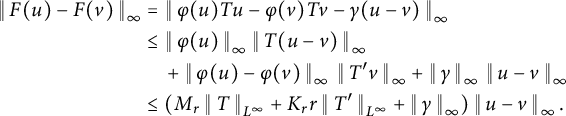 $$ \begin{align*} \left\lVert\,F(u) - F(v)\,\right\rVert_\infty & = \left\lVert\,\varphi(u)Tu - \varphi(v) Tv - \gamma (u-v)\,\right\rVert_{\infty} \\ & \leq \left\lVert\,\varphi(u)\,\right\rVert_\infty \left\lVert\,T(u-v)\,\right\rVert_\infty \\ &\quad +\left\lVert\,\varphi(u) -\varphi(v)\,\right\rVert_\infty \, \left\lVert\,T' v\,\right\rVert_\infty + \left\lVert\,\gamma\,\right\rVert_\infty \, \left\lVert\,u-v\,\right\rVert_\infty \\ & \leq (M_r \left\lVert\,T\,\right\rVert_{L^\infty} + K_r r \left\lVert\,T'\,\right\rVert_{L^\infty} + \left\lVert\,\gamma\,\right\rVert_\infty ) \left\lVert\,u-v\,\right\rVert_\infty. \end{align*} $$
This concludes the proof of Point (1).
We prove Point (2) in a similar way. Let
 $u, v \in \Delta $
. We have
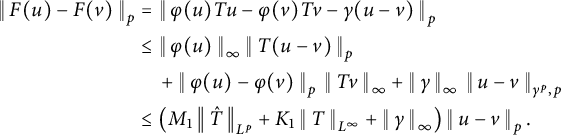 $$ \begin{align*} \left\lVert\,F(u) - F(v)\,\right\rVert_{p} & = \left\lVert\,\varphi(u)Tu - \varphi(v) Tv - \gamma (u-v)\,\right\rVert_{p} \\ & \leq \left\lVert\,\varphi(u)\,\right\rVert_\infty \left\lVert\,T(u-v)\,\right\rVert_{p} \\ &\quad +\left\lVert\,\varphi(u) -\varphi(v)\,\right\rVert_{p} \, \left\lVert\,T v\,\right\rVert_\infty + \left\lVert\,\gamma\,\right\rVert_\infty \, \left\lVert\,u-v\,\right\rVert_{\gamma^p,p} \\ & \leq \left(M_1 \left\lVert\,\hat{T}\,\right\rVert_{L^p} + K_1 \left\lVert\,T\,\right\rVert_{L^\infty} + \left\lVert\,\gamma\,\right\rVert_\infty \right) \left\lVert\,u-v\,\right\rVert_{p}. \end{align*} $$
This concludes the proof of Point (2).
For simplicity, we assume that
 $(h_n)_{n \in {\mathbb {N}}}$
is non-decreasing. Thus it converges a.e. (that is, in
 $L^0$
) to a limit, say h, and this limit belongs to
 $\Delta $
. Since T is positive, we also get that the sequence
 $(Th_n)_{n \in {\mathbb {N}}}$
is non-decreasing and bounded by
 , thus it converges a.e. (that is, in
 $L^0$
) to a limit, say
 $w\in L^\infty $
. On the other hand, by dominated convergence, we also get that
 $(h_n)_{n \in {\mathbb {N}}}$
converges to h in
 $L^p$
, and thus, as
 $\hat {T}$
is bounded on
 $L^p$
, we get that
 $(\hat {T} h_n)_{n \in {\mathbb {N}}}$
converges to
 $\hat {T} h$
in
 $L^p$
. We thus deduce that
 $w=\hat {T} h= Th$
. Then use that
 $\varphi $
is continuous, to deduce that
 $(F(h_n))_{n\in {\mathbb {N}}}$
converges a.e. to
 $F(h)$
. This gives Point (3).
We now prove that F is cooperative, see (7.4), using that
 $\varphi $
is nonnegative on
 $[0, 1]$
.
Lemma 8.2 (F is cooperative)
The map F is cooperative on
 $\Delta \times L^\infty $
and on
 $L^\infty \times \Delta $
.
Proof We first prove that F is cooperative on
 $\Delta \times L^{\infty }$
. Let
 $u\in \Delta $
and
 $v\in L^\infty $
with
 $u \leq v$
. Let
 $\nu \in L^{\infty , \star }_+$
such that
 $\langle \nu , u-v \rangle = 0$
. Since
 $v-u \geq 0$
, we deduce that for any
 $h\in L^\infty $
:
 $$ \begin{align} \langle \nu, (u-v)h \rangle = 0 \end{align} $$
(see [Reference Delmas, Dronnier and Zitt17, Lemma 2.6] for a proof in a very similar setting). Then, using (8.1) with
 $h=\gamma $
, we get
 $$\begin{align*}\langle \nu, F(u) - F(v) \rangle = \langle \nu, \varphi(u) Tu - \varphi(v) Tv - \gamma (u-v) \rangle = \langle \nu, \varphi(u) Tu - \varphi(v) Tv \rangle .\end{align*}$$
For
 $s, t\in {\mathbb {R}}_+$
, we set
 $\Phi (s,t)=(\varphi (s) -\varphi (t))/(s-t)$
if
 $s\neq t$
and
 $\Phi (s,s)=0$
. We have
 $$\begin{align*}\varphi(u) Tu - \varphi(v) Tv = \varphi(u) T(u-v) + (u-v) h \quad\text{with}\quad h=\Phi(u,v)\, Tv. \end{align*}$$
As
 $\varphi $
is locally-Lipschitz by Assumption 1 and as
 $u,v$
, and
 $Tv$
belong to
 $L^\infty $
, we deduce that
 $h\in L^\infty $
. We deduce from (8.1) that
 $$ \begin{align} \langle \nu, F(u) - F(v) \rangle = \langle \nu, \varphi(u) T(u-v) \rangle. \end{align} $$
As we have
 $\varphi \geq 0$
on
 $[0, 1]$
by Assumption 1 and
 $u \leq v$
, we have
 $\varphi (u) T(u-v) \leq 0$
. Thus, as
 $\nu $
is a positive linear form on
 $L^\infty $
, we have
 $\langle \nu , F(u) - F(v) \rangle \leq 0$
. Therefore, the map F is cooperative on
 $\Delta \times L^{\infty }$
.
If
 $(u,v)\in L^{\infty } \times \Delta $
satisfy
 $u\leq v$
, then using similar computations with
 $h=\Phi (v,u) T u$
, one get instead of (8.2) that
 $ \langle \nu , F(u) - F(v) \rangle = \langle \nu , \varphi (v) T(u-v) \rangle $
. Similar arguments yields then that F is also cooperative on
 $L^{\infty } \times \Delta $
.
Mimicking the proof of [Reference Delmas, Dronnier and Zitt17, Proposition 2.7(i)] (which in particular uses that
 $\varphi (1)=0$
), we get that any solution of (1.2) with an initial condition in
 $\Delta $
remains in
 $\Delta $
.
Lemma 8.3 The domain
 $\Delta $
is forward invariant for the differential equation
 $u'=F(u)$
in
 $L^\infty $
.
We then conclude on the existence of global solutions in
 $\Delta $
.
Lemma 8.4 (Maximal solutions are global)
Any maximal solution of
 $u'=F(u)$
in
 $L^\infty $
with initial condition
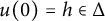 $u(0)=h\in \Delta $
is global.
Proof The bounded open set
 $U = \{f \in L^\infty \, \colon \, \left \lVert \,f\,\right \rVert _\infty < 2 \}$
of
 $L^\infty $
contains
 $\Delta $
, and the map F is Lipschitz on U by Lemma 8.1 (1). As the set
 $\Delta $
is forward invariant by Lemma 8.3, one can apply [Reference Lang33, Corollary IV 1.8] to conclude that any maximal solution to
 $u'=F(u)$
with initial condition in
 $\Delta $
is global.
Under Assumption 1, using Picard–Lindelöf theorem [Reference Lang33, Corollaries IV 1.6-8] and Lemma 8.4, which ensure the existence and uniqueness of maximal solution to
 $u'=F(u)$
in
 $L^\infty $
with initial condition in
 $\Delta $
, we can define the semi-flow
 $\phi \, \colon \, {\mathbb {R}}_+ \times \Delta \rightarrow \Delta $
, where the
 $L^\infty $
-valued function
 $\phi (\cdot , h)=( \phi (t, h))_{t\in {\mathbb {R}}_+}$
is the global solution to (1.2) with initial condition
 $u_0=h\in \Delta $
. Notice that
 $\phi (\cdot , h)$
belongs to
 $ \mathcal {C}^1({\mathbb {R}}_+)$
and satisfies the semi-group property:
 $$ \begin{align} \phi(t+s, h)=\phi(t, \phi(s, h)) \quad\text{for all}\quad s,t \in {\mathbb{R}}_+ \quad\text{and}\quad h\in \Delta. \end{align} $$
8.2 Properties of the semi-flow
We now establish the following properties of the semi-flow. We stress in the next lemmas that Assumption 1 holds.
Lemma 8.5 (Properties of the semi-flow)
Let
 $(T, \gamma , \varphi )$
satisfy Assumption 1.
-
(1) If
$h_1 \leq h_2$
belong to
$\Delta $
, then we have
$\phi (t,h_1) \leq \phi (t,h_2)$
for all
$t \in {\mathbb {R}}_+$
. -
(2) Let
$h \in \Delta $
. The function
$t \mapsto \phi (t,h)$
from
${\mathbb {R}}^+$
to
$L^\infty $
is non-decreasing (resp. non-increasing) if and only if we have
(resp.
) in
$L^\infty $
. -
(3) Let
$t\in {\mathbb {R}}_+$
. The function
$h\mapsto \phi (t, h)$
defined on
$\Delta $
is Lipschitz with respect to
$\left \lVert \,\cdot \,\right \rVert _\infty $
. -
(4) Let
$t\in {\mathbb {R}}_+$
. The function
$h \mapsto \phi (t, h)$
defined on
$\Delta $
is continuous with respect to the a.e. convergence, and, more generally, if
$(h_r)_{ r\in {\mathbb {R}}_+}$
is a sequence of elements of
$\Delta $
such that
$h=\operatorname *{\mbox {lim ess}} _{r\rightarrow +\infty } h_r$
exists (and thus belongs to
$\Delta $
), then
$\operatorname *{\mbox {lim ess}} _{r\rightarrow +\infty } \phi (t, h_r)=\phi (t, h)$
.








Proof For all the Points but (3), the proof mimics, respectively, the proofs of Propositions 2.8, 2.10, and 2.11 (ii) from [Reference Delmas, Dronnier and Zitt17]. Following the proof of Proposition 2.11 (iii) in [Reference Delmas, Dronnier and Zitt17], we see that to get Point (3), it is enough to check the following claim: if
 $(h_n)_{n\in {\mathbb {N}}}$
is a monotonous sequence of elements of
 $\Delta $
, which thus converges a.e. to a limit, say
 $h\in \Delta $
, then
 $(\phi (t, h_n))_{n\in {\mathbb {N}}}$
converges also a.e. to
 $\phi (t,h)$
for all
 $t\geq 0$
.
For simplicity, we assume that the sequence
 $(h_n)_{n\in {\mathbb {N}}}$
is non-decreasing. From Point (1), we get that the sequence
 $(\phi (s, h_n))_{n\in {\mathbb {N}}}$
is also non-decreasing and thus converges a.e. to a limit say
 $f_s\in \Delta $
for all
 $s\in {\mathbb {R}}_+$
. We deduce from Lemma 8.1 (3) that
 $(F(\phi (s, h_n)))_{n\in {\mathbb {N}}}$
converges a.e. toward
 $F(f_s)$
. Since F is bounded on
 $\Delta $
(as it is locally Lipschitz on
 $L^\infty $
) we deduce that the convergence also holds in
 $L^p$
. Since the identity map from
 $(L^\infty , \left \lVert \,\cdot \,\right \rVert _\infty ) $
to
 $(L^p, \left \lVert \,\cdot \,\right \rVert _{ p } )$
is continuous, we deduce that a solution to (1.2) in
 $L^\infty $
is also a solution to (1.2) in
 $L^p$
. By the fundamental theorem of calculus, see (7.2), we get that for all
 $s\geq 0$
:
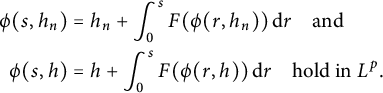 $$\begin{align*} \phi(s,h_n) &= h_n+ \int_0^s F(\phi(r, h_n))\, \mathrm{d} r \quad\text{and} \\ \phi(s,h) &= h+ \int_0^s F(\phi(r, h))\, \mathrm{d} r \quad\text{hold in } L^p. \end{align*}$$
By the dominated convergence Theorem 7.1 (with
 $X=L^p$
and g the constant function on
 ${\mathbb {R}}_+$
equal to 1), we deduce that
 $(f_s)_{s\in {\mathbb {R}}_+}$
is Bochner integrable on bounded intervals of
 ${\mathbb {R}}_+$
and for all
 $s\geq 0$
:
 $$\begin{align*}f_s = h+ \int_0^s F(f_r)\, \mathrm{d} r \quad\text{holds in } L^p. \end{align*}$$
We deduce from (7.1) and Lemma 8.1 (2) that for all
 $s\geq 0$
:
 $$\begin{align*}\left\lVert\,f_s - \phi(s,h)\,\right\rVert_{ p } \leq C_p \int _0 ^s \left\lVert\,f_r - \phi(r,h)\,\right\rVert_{ p }\, \mathrm{d} r. \end{align*}$$
Since
 $f_r$
and
 $\phi (r,h)$
belong to
 $\Delta $
, we get that
 $\left \lVert \,f_r - \phi (r,h)\,\right \rVert _{ p }\leq 2$
, so that
 $r\mapsto \left \lVert \,f_r - \phi (r,h)\,\right \rVert _{ p }$
is locally
 $\nu $
-integrable. We deduce from the Grönwall’s inequality that
 $\left \lVert \,f_s - \phi (s,h)\,\right \rVert _{ p }=0$
for all
 $s\geq 0$
. This gives that
 $f_s=\phi (s,h)$
for all
 $s\geq 0$
, which proves the claim.
Following [Reference Delmas, Dronnier and Zitt17, Proposition 2.13], we prove that the limit of the semi-flow is an equilibrium.
Lemma 8.6 (Limits of the semi-flow are equilibria)
Let
 $(T, \gamma , \varphi )$
satisfy Assumption 1. Let
 $h \in \Delta $
. If
 $\operatorname *{\mbox {lim ess}}_{t \rightarrow +\infty } \phi (t, h)$
exists, then it belongs to
 $\Delta $
and is an equilibrium.
Proof Let
 $h^*=\operatorname *{\mbox {lim ess}}_{t \rightarrow +\infty } \phi (t, h)$
. By Lemma 8.5 (3) and by (8.3), we have for all
 $s \in {\mathbb {R}}_+$
that
 $$\begin{align*}\phi(s, h^*)=\phi(s, \operatorname*{\mbox{lim ess}}_{t\rightarrow +\infty } \phi(t, h)) = \operatorname*{\mbox{lim ess}}_{t\rightarrow +\infty } \phi(s, \phi(t, h))= \operatorname*{\mbox{lim ess}}_{t\rightarrow +\infty } \phi(t, h)= h^*. \end{align*}$$
Then use Lemma 8.5 (2) to get that
 $F(h^*)=0$
.
8.3 Proof of Proposition 3.1 and Lemma 3.2
Proof of Proposition 3.1
The solution to Equation (1.2) in
 $L^\infty $
with initial condition in
 $\Delta $
is given by the semi-flow
 $\phi $
(see Section 8.1 and Lemma 8.4 therein). This gives Point (1). Point (2) is Lemma 8.3.
Since
 by Assumption 1, we get by Lemma 8.5 (2) that the semi-flow
 is non-increasing. This implies that
 exists. By Lemma 8.6, we get that
 $g^*$
is an equilibrium. Let
 $h \in \Delta $
be an equilibrium. We have
 , thus by Lemma 8.5 (1) we have
 for all
 $t \geq 0$
. Taking the essential limit, we get
 $h \leq g^*$
. This gives Point (3).
Proof of Lemma 3.2
For
 $h \in L^\infty $
and
 $i=1,2$
, let
 $F_i(h) = \varphi _i(h) T_i(h) - \gamma _i h$
and let
 $\phi _i$
be the semi-flow of Equation (1.2) with the parameters
 $(T_i, \gamma _i, \varphi _i)$
. By assumption, we have
 $F_1(g^*_2) \geq F_2(g^*_2) = 0$
. Thus, by Lemma 8.5 (2), the semi-flow
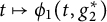 $t \mapsto \phi _1(t, g^*_2)$
is non-decreasing. By Lemma 8.6, since the essential limit
 $g=\operatorname *{\mbox {lim ess}}_{t\rightarrow +\infty } \phi _1(t, g^*_2)$
exists, it belongs to
 $\Delta $
and is an equilibrium (for the parameters
 $(T_1, \gamma _1, \varphi _1)$
). As
 $g^*_1$
is the maximal equilibrium, we have
 $g^*_1 \geq g$
, and thus
 $g^*_1 \geq g^*_2$
as the semi-flow
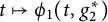 $t \mapsto \phi _1(t, g^*_2)$
is non-decreasing.
9 Proof of Proposition 4.3
9.1 On the support of the semi-flow
The following lemma is a generalization of [Reference Delmas, Dronnier and Zitt17, Lemma 4.10] where T is assumed to be irreducible.
Lemma 9.1 (Support of the semi-flow)
Let
 $(T, \gamma , \varphi )$
that satisfies Assumption 1 with
 $\varphi (0)>0$
. Let
 $h \in \Delta $
. We have
 $\operatorname {\mathrm {supp}}(\phi (t, h))=\mathcal {F}(\operatorname {\mathrm {supp}}(h))$
a.e. for all
 $t> 0$
.
Proof Since
 $\varphi (0)>0$
, there exists
 $a,\eta \in (0, 1)$
such that
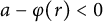 $a-\varphi (r)<0$
for all
 $r\in [0, \eta ]$
. Notice the operator
 $Q=aT -\gamma + \left \lVert \,\gamma \,\right \rVert _\infty $
on
 $L^\infty $
is positive and that the invariant sets for Q and T are the same. Set
 $f=\eta h/2$
and
 $A=\operatorname {\mathrm {supp}}(h)=\operatorname {\mathrm {supp}}(f)$
. There exists
 $c> 0$
small enough such that for all
 $t \in [0,c]$
:
 $$ \begin{align} \exp({at \left\lVert\,T\,\right\rVert_{L^\infty} } )< 2. \end{align} $$
Set for
 $t \geq 0$
:
 $$ \begin{align} u(t) = \mathrm{e}^{t(a T-\gamma)} f= \mathrm{e}^{- \left\lVert\,\gamma\,\right\rVert_\infty t} \, \mathrm{e}^{tQ} f. \end{align} $$
By [Reference Delmas, Lefki and Zitt19, Corollary 5.7] applied to the operator Q, we get that
 $\operatorname {\mathrm {supp}}(u(t))=\operatorname {\mathrm {supp}}(u(t)\mathrm {e}^{\left \lVert \,\gamma \,\right \rVert _\infty \, t})=\mathcal {F}(A)$
for
 $t>0$
. Differentiating (9.2) leads to
 $$ \begin{align} u'(t) - F(u(t)) = (a - \varphi(u(t))) T u(t). \end{align} $$
We deduce from (9.1) and (9.2) that
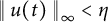 $\left \lVert \,u(t)\,\right \rVert _\infty <\eta $
for
 $t\in [0, c]$
, and thus, by definition of a and
 $\eta $
, that
 $ u'(t) - F(u(t))\leq 0$
for
 $t\in [0, c]$
. Then, since
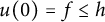 $u(0)=f\leq h$
, Theorem 7.2 implies that
 $u(t)\leq \phi (t, h)$
for
 $t \in [0,c]$
, and thus
 $\mathcal {F}(A)\subset \operatorname {\mathrm {supp}}(\phi (t, h))$
for
 $t\in (0, c]$
. Then, use the semi-flow equation (8.3) to propagate the result to all
 $t>0$
.
We deduce from Lemma 3.5 (3) that
 $\operatorname {\mathrm {supp}}(\phi (t,h)) =\operatorname {\mathrm {supp}}(\phi _{\mathcal {F}(A)}(t,h)) \subset \mathcal {F}(A)$
for all
 $t\geq 0$
. This gives that
 $\operatorname {\mathrm {supp}}(\phi (t,h)) = \mathcal {F}(A)$
for all
 $t> 0$
.
9.2 Preliminary results on the spectral radius and bound
We refer to [Reference Thieme52, Section 3] for results on the spectral bound on Banach lattices defined by (2.4).
Lemma 9.2 (Spectral radius and spectral bound)
Let
 $(T, \gamma , \varphi )$
that satisfy Assumption 2. Let
 $\delta : \Omega \rightarrow {\mathbb {R}}$
be a measurable positive function with
 $\delta \geq \gamma $
and
 $\operatorname *{\mbox {ess inf}} \delta> 0$
. Then, the quantities
 $s(T - \delta )$
,
 $s(\hat {T} - \delta )$
,
 $\rho (T_{1/\delta })-1$
, and
 $\rho (\hat {T}_{1/\delta })-1$
have the same sign.
Proof Notice that
 $(T, \delta , \varphi )$
also satisfies Assumption 2. By Lemma 2.8 (e) with
 $\gamma $
replaced by
 $\delta $
, we have that
 $\rho (\hat {T}_{1/\delta })=\rho (T_{1/\delta })$
. So it is enough to prove that
 $s(\hat {T} - \delta )$
and
 $\rho (\hat {T}_{1/\delta })-1$
have the same sign, and that
 $s(T - \delta )$
and
 $\rho (T_{1/\delta })-1$
have the same sign. This can be done by mimicking the proof of [Reference Delmas, Dronnier and Zitt17, Proposition 4.1] based on [Reference Thieme52], noticing that the cone
 $L^p_+$
is normal and reproducing for
 $p\in [1, +\infty ]$
, and that, by Lemma 2.8, the operators
 $\hat {T}_{1/\delta }$
and
 $T_{1/\delta }$
are, respectively, compact on
 $L^p$
and power compact on
 $L^\infty $
, and that the linear maps
 $\hat {T} - \delta $
and
 $T - \delta $
are operators, respectively, on
 $L^p$
and
 $L^\infty $
.
Adapting the proof of [Reference Delmas, Dronnier and Zitt17, Proposition 4.2] on kernel operators, we provide a weaker link between
 $\rho ( \hat {T}_{1/\gamma }) -1$
and
 $s(\hat {T} - \gamma )$
without the condition
 $\operatorname *{\mbox {ess inf}} \gamma> 0$
.
Proposition 9.3 (Positive spectral bound and Krein-Rutman theorem)
Let
 $(T, \gamma , \varphi )$
that satisfy Assumption 2. Then the following assertions are equivalent:
-
(1)
$s( T - \gamma )> 0$
or equivalently
$s(\hat {T} - \gamma )> 0$
. -
(2)
$\rho (T_{1/\gamma })> 1$
or equivalently
$\rho (\hat {T}_{1/\gamma })>1$
. -
(3) There exists
$\lambda> 0$
and
such that we have
$Tw - \gamma w = \lambda w$
.
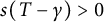
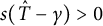


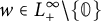

Proof Recall Assumption 2 holds and
 $p\in (1, +\infty )$
. Since
 $s(A-(\gamma +\varepsilon ))=s(A -\gamma ) -\varepsilon $
for
 $\varepsilon \in {\mathbb {R}}$
and A equal to T or
 $\hat {T}$
, we deduce from Lemma 9.2 that the two conditions in Point (1) are equivalent. We also deduce from Lemma 2.8 (e) that the two conditions in Point (2) are equivalent. So, we shall only consider the second ones. It is immediate that Point (3) implies Point (1) as
 $L^\infty \subset L^p$
and T and
 $\hat {T}$
coincide on
 $L^\infty $
.
We assume Point (1) and prove Point (3). For any
 $a\in {\mathbb {R}}_+$
, we denote
 $\psi (a) = \rho (V_a)$
with
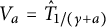 $V_a=\hat {T}_{1/(\gamma +a)}$
. Notice that
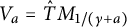 $V_a= \hat {T} M_{1/(\gamma +a)}$
for
 $a>0$
. By Assumption 2, the operator
 $V_a$
on
 $L^p$
is positive and that
 $V_a \geq V_b$
for
 $0\leq a\leq b$
. Thus the map
 $\psi $
is non-increasing on
 ${\mathbb {R}}_+$
by (2.5). By Point (1), there exists
 $\varepsilon> 0$
such that
 $s(\hat {T} - (\gamma + \varepsilon )) =s(\hat {T} - \gamma ) -\varepsilon> 0$
, therefore, we have
 $\psi (\varepsilon )> 1$
by Lemma 9.2 applied to
 $\delta = \gamma + \varepsilon $
. We thus get
 $\psi (0) = \rho (\hat {T}_{1/\gamma })> 1$
, that is Point (3).
We assume Point (3) and prove Point (3). By Point (3), we have
 $\psi (0)> 1$
. As for all
 $a> 0$
, we have
 $\psi (a) \leq \left \lVert \,V_a\,\right \rVert _{L^p} \leq a^{-1}\, \left \lVert \,\hat {T}\,\right \rVert _{L^p}$
. We deduce that
 $\lim _{a\rightarrow \infty }\psi (a) =0$
.
We now prove that
 $\psi $
is continuous on
 ${\mathbb {R}}_+$
. Let B denote the unit ball of
 $L^p$
. Notice that
 $M_{1/(\gamma +a)}(B) \subset M_{1/\gamma } (B)$
for
 $a\in {\mathbb {R}}_+$
and thus
 $\bigcup _{a\in {\mathbb {R}}_+} V_a(B)=V_0(B)=\hat {T}_{1/\gamma } (B)$
is relatively compact in
 $L^p$
, and thus the family
 $(V_a)_{a\in {\mathbb {R}}_+}$
is collectively compact. Thanks to Lemma 2.3, the continuity of
 $\psi $
holds if
 $ \lim _{|a-b| \rightarrow 0} \left \lVert \,(V_a -V_b)f\,\right \rVert _p=0$
for any
 $f\in L^p$
. This is indeed the case as, for
 $f\in L^p$
, we have
 $$\begin{align*}\left\lVert\,(V_a -V_b)f\,\right\rVert_p=\left\lVert\, \hat{T}_{1/\gamma} \left(\frac{(b-a)\gamma}{(\gamma+a) (\gamma+b)} f\right)\,\right\rVert_p \leq \left\lVert\, \hat{T}_{1/\gamma}\,\right\rVert_{L^p} \left\lVert\, \frac{(b-a)\gamma}{(\gamma+a) (\gamma+b)} f\,\right\rVert_p, \end{align*}$$
and the right members goes to
 $0$
as
 $|a-b|$
goes to
 $0$
using
 $|b-a|\gamma /(\gamma +a) (\gamma +b) \leq 1$
and dominated convergence. In conclusion, the function
 $\psi $
is continuous on
 ${\mathbb {R}}_+$
.
Since
 $\psi (0)> 1$
and
 $\lim _{a\rightarrow \infty }\psi (a) =0$
, we deduce from the continuity of
 $\psi $
, that there exists
 $\lambda> 0$
such that
 $\psi (\lambda ) = 1$
. Thus by the Krein–Rutman Theorem 2.5 (1) applied to the positive compact operator
 $V_\lambda $
on
 $L^p$
, there exists
 such that
 $V_\lambda v = v$
. Thanks to (1.6), we have
 $\left \lVert \,v\,\right \rVert _\infty =\left \lVert \,V_\lambda v\,\right \rVert _\infty \leq \left \lVert \,T(v/\gamma )\,\right \rVert _\infty \leq C^{\prime }_p \, \left \lVert \,v\,\right \rVert _p$
, we deduce that v belongs also to
 $L^\infty $
. Setting
 , we get that
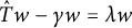 $\hat {T} w - \gamma w = \lambda w$
. As
 $\hat {T}$
and T coincide on
 $L^\infty $
, we get Point (3).
9.3 Proof of Proposition 4.3 (1)
Let g be a nonzero equilibrium. By Assumption 2,
 $\varphi (g) < 1$
on
 $\operatorname {\mathrm {supp}}(g)$
(as
 $\varphi (r) <1$
for
 $r\in (0, 1]$
). Recall the operator
 $S=\hat {T}_{1/\gamma }$
is compact on
 $L^p$
(see Lemma 2.8 (c)). Since
 $g\in \Delta $
is an equilibrium, we obtain that
 $$\begin{align*}S (\gamma g) = \frac{\gamma g}{\varphi(g)}> \gamma g \quad\text{on}\quad \operatorname{\mathrm{supp}}(g). \end{align*}$$
We deduce from Lemma 2.6 (2), with
 $\lambda =1$
, and (2.5) that
 $R_0 =\rho (S)\geq \rho \left (S_{\operatorname {\mathrm {supp}}(g)} \right )>1$
. In other words,
 $R_0\leq 1$
implies that
 is the only equilibrium. The last part of Point (1) is a consequence of Proposition 3.1 (3) and the monotonicity of the semi-flow from Lemma 8.5 (1).
9.4 Proof of Proposition 4.3 (2)
We assume that we have
 $R_0> 1$
. Similarly to [Reference Delmas, Dronnier and Zitt17, Section 4.4], we will prove that there exists a nonzero initial condition
 $w \in \Delta $
such that the semi-flow
 $\phi (., w)$
is non-decreasing. As
 $R_0> 1$
, there exists
 $a \in (0, 1)$
such that
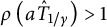 $\rho \left ( a\hat {T}_{1/\gamma } \right )> 1$
. Thus, by Proposition 9.3 (with
 $ (a T, \gamma , \varphi )$
), there exists
 $\lambda> 0$
and
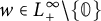 such that
 $a Tw - \gamma w = \lambda w$
. By Assumption 2, the map
 $\varphi $
is continuous with
 $\varphi (0) = 1$
; thus there exists
 $\eta \in (0,1)$
such that for all
 $r \in [0,\eta ]$
, we have
 $\varphi (r) \geq a$
. Without loss of generality, we assume that
 $\left \lVert \,w\,\right \rVert _\infty \leq \eta $
, and thus
 $w \in \Delta $
. We deduce that
 $$\begin{align*}F(w) = \varphi(w) Tw - \gamma w \geq aTw - \gamma w = \lambda w \geq 0. \end{align*}$$
By Lemma 8.5 (2), the semi-flow
 $t \mapsto \phi (t, w)$
is thus non-decreasing on
 ${\mathbb {R}}_+$
and its essential limit, say g, exists and belongs to
 $\Delta $
. It is an equilibrium by Lemma 8.6. Let
 $g^*$
denote the maximal equilibrium. As we have
 $g^*\geq g \geq w$
and
 $\mu (\operatorname {\mathrm {supp}}(w))> 0$
, we deduce that
 $\mu (\operatorname {\mathrm {supp}}(g^*))> 0$
.
9.5 Proof of Proposition 4.3 (3)
We now assume that
 $T = T_A$
with A an irreducible set. Notice the set A is invariant and thus admissible; and it has positive measure as
 $R_0>0$
. It is thus a (nonzero) atom by [Reference Delmas, Lefki and Zitt19, Theorem 1]. Let g be a nonzero equilibrium. We have
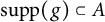 $\operatorname {\mathrm {supp}}(g) \subset A$
by (1.4). Since
 $\operatorname {\mathrm {supp}}(g)$
is invariant, see Lemma 4.1 (3), and A is an atom, we deduce that
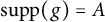 $\operatorname {\mathrm {supp}}(g)=A$
. Then use that the support of g characterizes g, see Corollary 4.2 to deduce that g is the only nonzero equilibrium.
9.6 Proof of Proposition 4.3 (4)
By Point (3), we have
 $\operatorname {\mathrm {supp}}(g^*) = A$
. On
 $A^c$
, we have
 $\phi (t,h)'= -\gamma \phi (t,h)$
, so that
 . So it is enough to prove the result when
 $\operatorname {\mathrm {supp}}(h)\subset \operatorname {\mathrm {supp}}(g^*) = A$
. As
 $\operatorname {\mathrm {supp}}(h)$
is a non-empty set included in the invariant and irreducible set A, its future is equal to A. Thus, by Lemma 9.1 and considering
 $\phi (1, h)$
instead of h, one can assume without loss of generality that
 $\operatorname {\mathrm {supp}}(h) = \operatorname {\mathrm {supp}}(g^*) = A$
.
For
 $\varepsilon \in (0, 1]$
, we consider the operator
 $U_\varepsilon =\varphi (\varepsilon ) M_{\{h\geq \varepsilon \}} \hat {T}_{1/\gamma }$
on
 $L^p(\mu )$
, and set
 $U_0=M_{\{h>0\}} \hat {T}_{1/\gamma }$
. Let B be the unit ball in
 $L^p$
. Since
 $\hat {T}_{1/\gamma }$
is compact and
 a.e., we deduce that
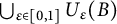 $\bigcup _{\varepsilon \in [0, 1]} U_\varepsilon (B)$
is relatively compact. Thus the family of operators
 $(U_\varepsilon )_{\varepsilon \in [0,1]}$
is collectively compact. By dominated convergence, we also get that
 $\lim _{\varepsilon \rightarrow 0} \left \lVert \,(U_\varepsilon -U_0) f\,\right \rVert _p=0$
. We deduce from Lemma 2.3 that the map
 $\varepsilon \mapsto \rho (U_\varepsilon )$
is continuous at
 $0$
. Thus, there exists
 $\varepsilon \in (0,1)$
such that
 $\rho (U_\varepsilon )> 1$
. Notice that
 satisfies Assumption 2. By Proposition 9.3 with T replaced by
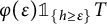 , there exists
 $\lambda> 0$
and
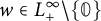 such that

Without loss of generality, we can assume that
 $\left \lVert \,w\,\right \rVert _\infty \leq \varepsilon $
. We also have
 $$ \begin{align} \operatorname{\mathrm{supp}}(w) \subset \{h\geq \varepsilon\} \subset A. \end{align} $$
Using (9.4) we get that
 $$ \begin{align} F(w)=\varphi(w) Tw - \gamma w\geq \varphi(\varepsilon) Tw - \gamma w \geq \lambda w\geq 0. \end{align} $$
We deduce that the map
 $t \mapsto \phi (t,w)$
is non-decreasing by Lemma 8.5 (2) and, as
 $g^*$
is the only nonzero equilibrium, that
 $\operatorname *{\mbox {lim ess}}_{t\rightarrow \infty } \phi (t, w)=g^*$
by Lemma 8.6. As the semi-flow is monotone by Lemma 8.5 (1), we deduce that
 for all
 $t\in {\mathbb {R}}_+$
. Then, use Proposition 3.1 (3) to conclude that
 $\operatorname *{\mbox {lim ess}}_{t\rightarrow \infty } \phi (t, h)=g^*$
.
10 Proof of Theorem 5.1
Let
 $(T, \gamma , \varphi )$
that satisfy Assumption 2. We keep notations from Section 4; so
 $\mathcal {C}_A$
is the supercritical antichain given by the maximal elements of the supercritical atoms included in the set A.
Proof of Theorem 5.1
Let
 $A = \mathcal {F}(\operatorname {\mathrm {supp}}(h))$
and
 $g^*_A$
be the maximal equilibrium on A (notice that
 $A=\emptyset $
if
 ). Since A is invariant,
 $g^*_A$
is also an equilibrium by Lemma 3.4 (2).
We will, as in the proof of Proposition 4.3 (4), prove the existence of
 $w \in \Delta $
with
 $w \leq h$
such that the semi-flow
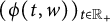 $(\phi (t, w))_{t\in {\mathbb {R}}_+}$
is non-decreasing and converges essentially to
 $g^*_A$
. By Lemma 9.1 and considering
 $\phi (1, h)$
instead of h, one can assume without loss of generality that
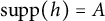 $\operatorname {\mathrm {supp}}(h) =A$
. If
 $\mathcal {C}_A$
is empty, we get that
 and by Lemma 3.5 (1) and (3), we have
 , and by monotonicity of the semi-flow that
 , which proves Theorem 5.1 in this case.
We now assume that
 $\mathcal {C}_A$
is not empty. Let
 $B\in \mathcal {C}_A$
. By considering
 $T_B$
instead of T, mimicking the proof of Proposition 4.3 (4), see (9.5) and (9.6), we deduce that there exists a function
 $w_B\in \Delta $
such that
 $\operatorname {\mathrm {supp}}(w_B)\subset B$
,
 $w_B\leq h$
,
 $F(w_B)\geq 0$
, and
 $\operatorname *{\mbox {lim ess}}_{t\rightarrow \infty } \phi _B(t,w_B)= g^*_B$
. Since
 $\mathcal {C}_A$
is an antichain of atoms, we deduce that
 $\mathcal {F}(\operatorname {\mathrm {supp}}(w_B))\cap \operatorname {\mathrm {supp}}(w_{B'})\subset \mathcal {F}(B) \cap B'=\emptyset $
for all
 $B', B\in \mathcal {C}_A$
such that
 $B\neq B'$
. Set
 $w=\sum _{B\in \mathcal {C}_A} w_B\leq h$
. We have

where for the first equality we used that
 $\mathcal {F}(B)$
is invariant and
 $\operatorname {\mathrm {supp}}(w_B) \subset B\subset \mathcal {F}(B)$
, and for the second that
 $\varphi (w)-\varphi (w_B)=0$
on
 $\mathcal {F}(B)$
for
 $B\in \mathcal {C}_A$
. Arguing as in the end of the proof of Proposition 4.3 (4), we deduce that the semi-flow
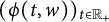 $(\phi (t,w))_{t\in {\mathbb {R}}_+}$
is non-decreasing and that
 $\operatorname *{\mbox {lim ess}}_{t\rightarrow \infty } \phi (t, w)=g\in \Delta $
with g an equilibrium.
We now prove the equality
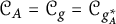 $\mathcal {C}_A = \mathcal {C}_g = \mathcal {C}_{g^*_A}$
. Since
 $w\leq g$
, we deduce that
 $\mathcal {C}_A \subset \mathcal {C}_g$
. Since
 $\operatorname {\mathrm {supp}}(w) \subset A$
and A is invariant, we have
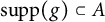 $\operatorname {\mathrm {supp}}(g) \subset A$
by Lemma 9.1. In particular, g is an equilibrium of A by Lemma 3.4 (1), thus we get
 $g \leq g^*_A$
and deduce that
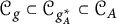 $\mathcal {C}_g \subset \mathcal {C}_{g^*_A}\subset \mathcal {C}_A$
as
 $\operatorname {\mathrm {supp}}(g^*_A) \subset A$
. This proves the claim and that
 $g=g^*_A$
by Corollary 4.2.
By monotonicity of the semi-flow, we have that
 for all
 $t \geq 0$
. The left term converges essentially to
 $g=g^*_A$
, and the right term to
 $g^*_A$
by Lemma 3.5. This gives
 $\operatorname *{\mbox {lim ess}}_{t\rightarrow \infty } \phi (t,h)=g^*_A$
. This ends the proof.