Historically, an important compromise that helped create the Electoral College was the addition of two electoral votes to each state regardless of population size (Harvard Law Review 2001). This compromise was made to assure less populous states a proportionally greater influence in electing the president. The winner-take-all methodology of awarding electoral votes, currently used by all states except Maine and Nebraska, is generally acknowledged to give more populous states an advantage in determining the outcome of presidential elections (Harvard Law Review 2001; Longley and Dana Reference Longley and Dana1984; Sterling Reference Sterling1978). Grofman, Brunell, and Campagna (Reference Grofman, Brunell and Campagna1997) express a generally accepted perception: “The electoral college operates to create the illusion of a popular mandate.” Indeed, the Electoral College's average margin of victory of 273.19 electoral votes observed in presidential elections from 1900 through 2000 (http://www.archives.gov) did create the “illusion” of large popular mandates in the majority of those elections. We performed this analysis to quantify the advantage given to the winner as a result of the two electoral vote add-on (a constitutional rule) and the winner-take-all (an individual state rule) methodologies used in the Electoral College.

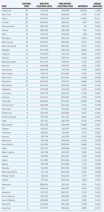
In order to quantify the two electoral vote add-on advantage to the winner, we generated one million random two-candidate simulated elections using the electoral vote distribution for the 50 states and the District of Columbia that existed for the 2000 U.S. presidential election. We randomly assigned the electoral votes of each of the 50 states and the District of Columbia with equal likelihood to one of two candidates. If A was the number of electoral votes won by candidate A and B was the number of electoral votes won by candidate B, then the equation A + B = 538 was valid for each of these two-candidate simulated elections. If A, by definition, was the “winner,” then A must be 270 or more. Individual state results for these one million simulated elections are shown in Table 1. For example, California, with 54 electoral votes, voted for the winner 729,545 times out of the one million election simulations. Wyoming, with three electoral votes, voted for the winner 507,377 times out of the one million election simulations. A 269 to 269 electoral vote tie occurred 7,630 times. In order to assess the advantage of the two electoral vote add-on, we recalculated these simulated election results without it. We also used this recalculation to determine how often the outcome of these random simulated elections would have been reversed if the two electoral vote add-on did not exist. For example, if A won X number of states and B won Y number of states, then how often was the equation A − 2X < B − 2Y satisfied? That equation was satisfied 25,482 times out of the one million simulated elections.

Table 1.

Table 1

The results of these recalculations, without the two electoral vote add-on, are also shown in Table 1. Without the two electoral vote add-on, California, now with 52 electoral votes, would have voted for the winner 749,094 times out of one million. Wyoming, with one electoral vote, would have voted for the winner 499,522 times out of the one million. Table 1 also lists the difference in the number of times each state voted for the winner when taking into consideration the two electoral vote add-on. For example, California voted for the winner 19,549 fewer times, while Wyoming voted for the winner 7,855 more times. We calculated the average electoral vote advantage given to the winner due to the two electoral vote add-on per election by multiplying the differences in wins shown in Table 1 by the corresponding number of electoral votes for that electoral entity (with the two electoral vote add-on), summing these products for the 51 electoral entities, and then dividing that sum by one million, the number of simulated elections. The intrinsic advantage for the winner as a result of the two electoral vote add-on methodology was 0.42 electoral votes per election. That is, the two electoral vote add-on added an average of 0.42 electoral votes to the winner's total electoral vote count. Similarly, we also calculated the average advantage given to the winner per election due to the two electoral vote add-on for each individual state by multiplying the difference in wins for that entity by the number of electoral votes that that entity has (with the two electoral vote add-on) and then dividing that product by one million, the number of simulated elections. As shown in Table 1, California loses an average of 1.056 electoral votes per election and Wyoming gains an average 0.024 electoral vote per election. As shown in Table 1, the advantage given to the winner due to the two electoral vote add-on was positive to all electoral entities except for the four states with the most electoral votes: California, New York, Texas, and Florida. States with nine to 14 electoral votes actually had the largest advantage given to the winner. Thus, the two electoral vote add-on does not specifically confer the largest advantage to the winner from the least populous states.

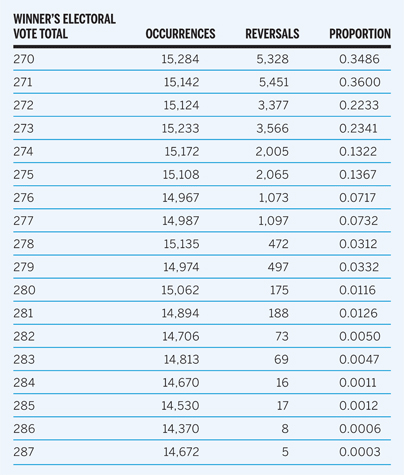
Although the two electoral vote add-on advantage to the winner in these simulated elections is small in terms of average absolute electoral votes, the two electoral vote add-on methodology altered the outcome of these simulated presidential elections over 2.5% of the time (25,482 times out of one million random simulated elections in this study). The distribution of the winner's total electoral votes in these 25,482 simulated elections is listed in Table 2. As shown in Table 2, the likelihood of reversal of an election outcome rapidly declines as the winner's total electoral vote count increases. No election reversal due to the two electoral vote add-on occurred in this analysis when the winner obtained 288 or more electoral votes. In actual U.S. presidential elections from 1900 through 2000, two outcomes (those of the 1916 and 2000 presidential elections) would have been reversed if the two electoral vote add-on did not exist (http://www.archives.gov). Thus, the two electoral vote add-on actually altered the outcome in two of 26 (about 7.7%) presidential elections from 1900 through 2000. The observation that the two electoral vote add-on has actually altered presidential election outcomes at three times the rate expected in these simulations suggests that this Electoral College rule exerts a greater influence than suggested by the average 0.42 electoral votes given to the winner in this simulation study.

Table 2.

Table 2

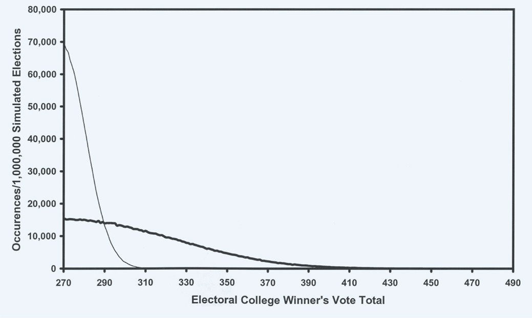
In this study, Maine and Nebraska were assumed to use the winner-take-all methodology. We calculated the average winning electoral vote total by multiplying the number of wins with the two electoral vote add-on for each electoral entity shown in Table 1 by the number of electoral votes that each entity possessed, summing these 51 products, and then dividing that sum by one million, the number of simulated elections. The result of this calculation was that the winner's average electoral vote total was 307.69 electoral votes. By comparison, the average winner's electoral vote total was 397.54 votes in actual presidential elections from 1900 through 2000. The distribution of the winner's total electoral votes for the one million randomly generated two-candidate simulated elections, using the electoral vote distribution for the 50 states and the District of Columbia that existed for the 2000 presidential election, is shown by the thick line in Figure 1.

Figure 1.

Figure 1

In order to assess the advantage to the winner of the winner-take-all methodology, we generated an additional one million random two-candidate simulated elections using 538 single electoral vote entities. This simulation assumed that each electoral vote was independent of every other electoral vote and was equally likely to go to either of the two candidates. The distribution of the winner's total electoral votes for these simulations is shown by the thin line in Figure 1. Thus, the impact of the winner-take-all methodology, as shown in Figure 1, is to spread out the distribution of the winner's electoral vote total, resulting in a greater expected average of the winner's electoral vote total. Of note, a 269 to 269 electoral vote tie occurred 34,059 times in these one million single electoral vote election simulations. We then determined the average winning total for this second simulation by summing the electoral vote total for the winner in each of the one million elections and then dividing that sum by one million. The winner's average electoral vote total for the one million two-candidate simulated elections generated using 538 single electoral vote entities was 278.24 electoral votes. We subtracted the average winning electoral vote total for these 538 independent single electoral vote simulated elections from the average winning electoral vote total for the one million simulated elections using the winner-take-all methodology. This subtraction gave the winner's average advantage per election due to the winner-take-all methodology. Thus, compared to an Electoral College that allowed each of the 538 electoral votes to be won or lost individually, an Electoral College that utilized the winner-take-all methodology added an average of 29.45 (from 307.69 minus 278.24) electoral votes to the winner's total (this is for the 51 electoral entities with the distribution of electoral votes present in the 2000 U.S. presidential election). The 0.42 electoral vote advantage given to the winner as a result of the two electoral vote add-on methodology is embedded within the 29.45 electoral vote advantage to the winner resulting from the winner-take-all methodology.

Previous studies of bias in the Electoral College have focused on such factors as swing ratio, partisan bias, and unequal voter representation per electoral vote between the various states (Berthoud Reference Berthoud1997; Brams and Davis Reference Brams and Davis1974; Destler Reference Destler1996; Garand and Parent Reference Garand and Parent1991; Grofman, Brunell, and Campagna Reference Grofman, Brunell and Campagna1997; Harvard Law Review 2001; Holbrook and Van Dunk Reference Holbrook and Van Dunk1993; Longley and Dana Reference Longley and Dana1984; Nelson Reference Nelson1974; Shaw Reference Shaw1999; Sterling Reference Sterling1978). We specifically and purposefully used the simulation strategy in this analysis so as to eliminate the influence that such factors as swing ratio, partisan bias, and unequal voter representation would have on the outcome of two-candidate elections. Each electoral entity's votes were equally likely to be won by either of the two candidates. Such concepts as popular vote, percentage of popular vote obtained by either candidate in any state, or tendency of a particular state to prefer to a particular political party's candidate had no relevance. This analysis specifically, and only, addressed the question of how much does the winner-take-all and the two electoral vote add-on methodologies increase the winner's expected margin of victory in the Electoral College.

The results of this analysis demonstrate that the rules of the Electoral College give the winning candidate an average of 29.45 additional electoral votes per election due to the winner-take-all methodology, including the winner's 0.42 electoral vote advantage. Consequently, the Electoral College's two methodologies create an additional average expected margin of victory of 58.90 electoral votes (29.45 multiplied by two). If each of the 538 electoral votes were awarded randomly, singularly, and independently to one of two candidates, the advantage to the winner of that voting system was 9.24 electoral votes for an expected average margin of victory of 18.48 electoral votes (9.24 multiplied by two). Thus, the average expected margin of victory in the Electoral College would be 77.38 electoral votes (58.90 plus 18.48). This winner's advantage is much smaller than the popular mandate suggested by the average margin of victory of 273.19 electoral votes observed in actual presidential elections from 1900 through 2000 (http://www.archives.gov). Thus, the large popular mandate implied by the results in most twentieth-century presidential elections can not be solely attributed to the rules employed by the Electoral College.

Our findings demonstrate that both the two electoral vote add-on and winner-take-all methodologies produce the same basic effect. That is, both methodologies clump electoral votes and increase the winner's expected average margin of victory in two-candidate elections. Even without this clumping, a small winner's advantage occurs. In only three presidential elections between 1900 and 2000, the elections of 1916, 1976, and 2000 (http://www.archives.gov), was the margin of victory less than 77.38 electoral votes. Of note, the 2004 presidential election was also very close with a margin of victory of 35 electoral votes (http://www.archives.gov). Despite these observations, one should not conclude that the methodologies utilized by the Electoral College have not impacted the outcome of presidential elections. As noted, of the one million randomly generated presidential elections, the outcome would have been reversed 25,482 times if the two electoral vote add-on did not exist. The outcomes of the 1916 and 2000 presidential elections would have been reversed without the two electoral vote add-on (http://www.archives.gov). In 1916, Wilson beat Hughes by an electoral vote of 277 to 254. Wilson won 30 states. Hughes won 18 states. Without the add-on, Hughes would have won the election by a single electoral vote, 218 (from 254 − 18[2]) to 217 (from 277 − 30[2]). In 2000, Bush beat Gore with 271 electoral votes to Gore's 266 electoral votes (a single District of Columbia elector abstained). Bush won 30 electoral entities. Gore won 21 electoral entities. Consequently, without the two electoral vote add-on, Gore would have won the presidential election by an electoral vote of 224 (from 266 − 21[2]) to 211 (from 271 − 30[2]). Of note, the outcome of the close 2004 presidential election would not have been reversed without the two electoral vote add-on. As observed in most forms of competition, the rules of the game become relatively more important in close contests. While acknowledging that these rules have impacted the outcome of some presidential elections, we don't intend to offer a suggestion for reform of the Electoral College by this analysis. A constitutional amendment would be required to change the two electoral vote add-on rule. Individual states are free to change the winner-take-all rule, as Maine and Nebraska have already done.

Ties are much less likely to occur when electoral votes are awarded in blocks. A 269 to 269 electoral vote tie occurred only 7,630 times in the one million election simulations when using the 2000 election's electoral vote distribution. A 269 to 269 electoral vote tie occurred 34,059 times in the one million election simulations in which the votes were awarded individually and independently. The clumping of electoral votes, as existed for the 2000 presidential election, makes Electoral College vote ties almost 4.5 times less likely to occur.

Finally, this analysis was based upon the distribution of electoral votes that existed for the 2000 U.S. presidential election, an arbitrary point in time. A similar analysis could have been performed based on the electoral vote distribution that existed at the time of any other presidential election. The total electoral votes in the Electoral College has changed over time. The electoral vote distribution among the various states has and will continue to change, reflecting changes in the decennial census. Thus, although the actual expected winner's advantage due to the rules of the Electoral College will vary slightly over time, the winner's advantage based on the two electoral vote add-on and the winner-take-add rules will and, mathematically, must persist.