1 Introduction
The possibility of using wings with wavy leading edges as a way of obtaining improved aerodynamic performance started to receive attention after the work of Fish & Battle (Reference Fish and Battle1995), where the morphology of the pectoral flipper of the humpback whale (Megaptera novaeangliae) was analysed, with a focus on its hydrodynamic performance. These flippers have protuberances on the leading edge, and it was suggested that these act as a mechanism to delay the stall, allowing the flipper to maintain a high lift coefficient at high angles of attack, giving the whale good manoeuvrability.
The idea that leading edge protuberances could delay stall gained support with the work of Miklosovic et al. (Reference Miklosovic, Murray, Howle and Fish2004) and Miklosovic, Murray & Howle (Reference Miklosovic, Murray and Howle2007). They presented experiments for full-span and half-span wings with a NACA0020 profile in configurations with and without leading edge waviness. For the half-span model, which had a planform similar to the flipper of the humpback whale, the Reynolds number was around
 $6\times 10^{5}$
and the modified wing led to an increase in the stall angle. This increase in the stall angle contributed to an increase in the maximum lift coefficient of the wing. However, for the full-span model, for which the Reynolds number was around
 $2.7\times 10^{5}$
, their results showed that the protuberances lead to a premature stall, being beneficial only in the post-stall regime. Moreover, the experiments for full-span wings presented in Johari et al. (Reference Johari, Henoch, Custodio and Levshin2007) showed the same behaviour, with the modified leading edge causing a premature stall.
Although these first studies on the effect of leading edge protuberances showed a strong distinction between the behaviour of full-span and half-span models, more recent works suggest that the main factor affecting the results could be the Reynolds number,
 $Re$
. First, Stanway (Reference Stanway2008) presented experiments for a model similar to the half-span wing of Miklosovic et al. (Reference Miklosovic, Murray, Howle and Fish2004), but considering different values of
 $Re$
between
 $4\times 10^{4}$
and
 $1.2\times 10^{5}$
. Only for the highest value of
 $Re$
considered did the waviness cause an increase in the maximum lift coefficient, indicating that the value of
 $Re$
has an important role in determining whether the use of wavy leading edges will improve aerodynamic performance.
Another study that supports the importance of the Reynolds number effect on this flow is that of Hansen, Kelso & Dally (Reference Hansen, Kelso and Dally2010). They performed experiments with a rectangular wing mounted in both full-span and half-span configurations, in an attempt to isolate the influence of the wing tip on the results. The effect of using a wavy leading edge was similar in both cases, indicating that three-dimensional effects related to the wing tip have a secondary importance in the effectiveness of the waviness. Therefore, the effect of the waviness for infinite wings (as considered here) is expected to be similar to the effect for rectangular wings with a finite span. Three-dimensional effects from using different planforms may play a significant role, but this aspect was not explored in the present paper.
Despite the large number of studies on this topic, only a few have attempted to describe the flow in detail, explaining the mechanisms responsible for the changes in the aerodynamic forces caused by the waviness. Favier, Pinelli & Piomelli (Reference Favier, Pinelli and Piomelli2012) performed a parametric study based on numerical simulations of infinite wings with a NACA0020 profile for a very low Reynolds number,
 $Re=800$
, with a single angle of attack,
 $\unicode[STIX]{x1D6FC}=20^{\circ }$
. They describe the topology of this flow, observing separation regions behind the troughs, with attached flow behind the peaks. Skillen et al. (Reference Skillen, Revell, Pinelli, Piomelli and Favier2015) performed large-eddy simulations for a straight and a wavy infinite wing with
 $Re=120\,000$
, also with
 $\unicode[STIX]{x1D6FC}=20^{\circ }$
. They attribute the observed improvement in the aerodynamic performance to a reduction in the extent of separated flow, which is suggested to be caused by a secondary flow induced by the spanwise pressure gradient and by a strong flow acceleration between the waviness peaks. Rostamzadeh et al. (Reference Rostamzadeh, Hansen, Kelso and Dally2014) used experimental and numerical results with
 $Re=120\,000$
to explain the formation of counter-rotating streamwise vortices. They show that the presence of these vortices can be explained by two alternative mechanisms: the spanwise variation of spanwise vorticity or the skew-induced mechanism caused by the change in the streamline curvature near the wavy leading edge. They also analyse the flow topology, characterized by delta shaped separation regions. Still considering the streamwise vorticity, Hansen et al. (Reference Hansen, Rostamzadeh, Kelso and Dally2016) used experiments and numerical simulations with
 $Re=2230$
to determine the evolution of circulation and peak vorticity along the chord direction, also discussing the flow structures observed in this case of a laminar flow regime.
In a previous study (Serson, Meneghini & Sherwin Reference Serson, Meneghini and Sherwin2017), we presented numerical results for wavy infinite wings at
 $Re=1000$
. In that case, it was observed that the waviness leads to reductions in the aerodynamic forces, which are associated with a flow regime where separation is restricted to the waviness troughs. It was proposed that this is caused by the spanwise flow around the leading edge leading to a reduction in the suction peaks behind the sections corresponding to the waviness peaks, causing the flow to remain attached in these sections (because of a weaker adverse pressure gradient) but at the same time decreasing the ability of the wing to generate lift. In the present paper, a more extensive numerical investigation is presented, this time considering
 $Re=10\,000$
and
 $Re=50\,000$
at different angles of attack in both the pre-stall and post-stall regimes. These higher values of
 $Re$
are closer to what might be found in some applications, like micro air vehicles (Mueller & DeLaurier Reference Mueller and DeLaurier2003), and also allow comparisons with experimental results presented by Paula (Reference Paula2016). We describe the flow in detail, discussing how these results relate to the lower-
 $Re$
case, and also what new features can be observed as the flow moves towards a transitional regime.
The paper is organized as follows. Section 2 briefly presents the numerical methods employed in the simulations, while § 3 describes the most important parameters used in the simulations. Then, § 4 presents the results, and finally § 5 contains the conclusions of this work.
2 Numerical methods
We consider an incompressible viscous flow, which is governed by the Navier–Stokes equations. Assuming a unit density, these equations can be written as
 $$\begin{eqnarray}\displaystyle \left.\begin{array}{@{}c@{}}\displaystyle \frac{\unicode[STIX]{x2202}\boldsymbol{u}}{\unicode[STIX]{x2202}t}=-(\boldsymbol{u}\boldsymbol{\cdot }\unicode[STIX]{x1D735})\boldsymbol{u}-\unicode[STIX]{x1D735}p+\unicode[STIX]{x1D708}\unicode[STIX]{x1D6FB}^{2}\boldsymbol{u},\\ \displaystyle \unicode[STIX]{x1D735}\boldsymbol{\cdot }\boldsymbol{u}=0,\end{array}\right\} & & \displaystyle\end{eqnarray}$$
where
 $\boldsymbol{u}$
is the velocity,
 $p$
is the pressure and
 $\unicode[STIX]{x1D708}$
is the kinematic viscosity. Taking the chord
 $c$
as the reference length and the free-stream velocity
 $U_{\infty }$
as the reference velocity, the Reynolds number is defined as
 $Re=cU_{\infty }/\unicode[STIX]{x1D708}$
.
The waviness of the wing was treated by a coordinate system transformation using the formulation proposed in Serson, Meneghini & Sherwin (Reference Serson, Meneghini and Sherwin2016), so that the wavy geometries were mapped into the straight wing. Then, the equations were discretized following the spectral/hp method presented in Karniadakis & Sherwin (Reference Karniadakis and Sherwin2005), with the span direction discretized using a Fourier expansion, as proposed by Karniadakis (Reference Karniadakis1990). The use of a Fourier expansion in the third direction is an efficient way of studying an infinite wing with periodic boundary conditions, and was only possible because of the simplification in the geometry provided by the coordinate transformation. The equations were then solved by time integration using the stiffly stable splitting scheme described by Karniadakis, Israeli & Orszag (Reference Karniadakis, Israeli and Orszag1991) and Guermond & Shen (Reference Guermond and Shen2003).
3 Simulation set-up
All numerical simulations presented here were performed using the incompressible Navier–Stokes solver encapsulated within the spectral/hp element code Nektar++ (Cantwell et al. Reference Cantwell, Moxey, Comerford, Bolis, Rocco, Mengaldo, Grazia, Yakovlev, Lombard and Ekelschot2015). The geometries are based on a NACA0012 profile, with a small modification to obtain a zero-thickness trailing edge, since the small thickness of the trailing edge in the original profile would lead to meshing challenges. The wavy geometries were obtained by applying the following coordinate transformation to the straight infinite wing:
 $$\begin{eqnarray}\displaystyle \bar{x}=x+\unicode[STIX]{x1D709}(z)=x-\frac{h}{2}\cos \left(\frac{2\unicode[STIX]{x03C0}}{\unicode[STIX]{x1D706}}z\right), & & \displaystyle\end{eqnarray}$$
where
 $h$
is the waviness peak-to-peak amplitude,
 $\unicode[STIX]{x1D706}$
is its wavelength,
 $\bar{x}$
is the physical coordinate in the chord direction, and
 $x$
and
 $z$
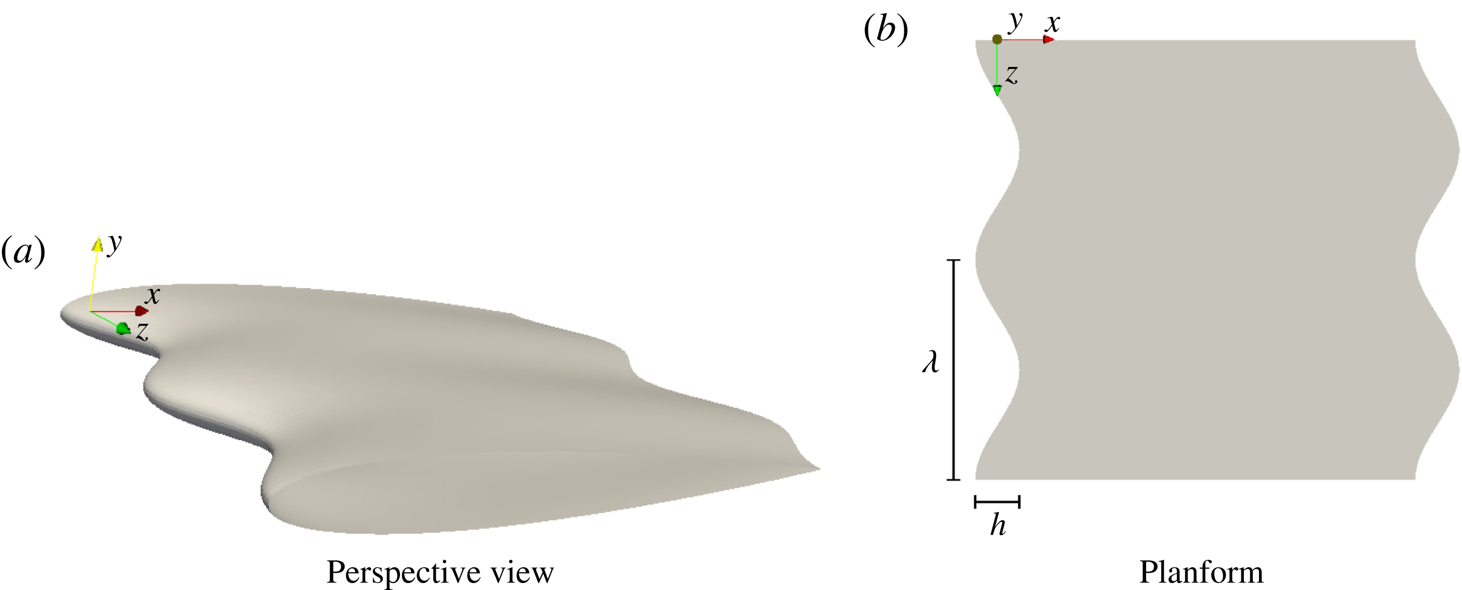
are the chordwise and spanwise coordinates in the computational domain. Figure 1 shows an example of a geometry obtained through this transformation, identifying the waviness parameters and the orientation and origin of the coordinate system. It should be noted that this transformation deforms both the leading and trailing edges, and has no effect on the chord. This type of transformation was preferred because it leads to a simpler procedure when solving the equations with the mapping (Serson et al.
Reference Serson, Meneghini and Sherwin2016). However, in Serson et al. (Reference Serson, Meneghini and Sherwin2017), it was shown that for this same geometry with
 $h=0.1c$
,
 $\unicode[STIX]{x1D706}=0.5c$
,
 $Re=1000$
and
 $0^{\circ }\leqslant \unicode[STIX]{x1D6FC}\leqslant 21^{\circ }$
, the effect on the aerodynamic forces and recirculation regions of deforming both the leading and trailing edges is almost identical to that of deforming only the leading edge. Therefore, we expect our results to be comparable to the ones available in the literature for wavy leading edges, at least in terms of forces and flow structures. The effect of the trailing edge shape may be relevant when the sound generated by the wing is of interest, which was not the case in the present study.
The geometry of a wavy wing with
 $h/c=0.1$
and
 $\unicode[STIX]{x1D706}/c=0.5$
.

We considered the case without any waviness (referred to as the baseline) and wavy geometries with three different combinations of the parameters
 $\unicode[STIX]{x1D706}$
and
 $h$
for
 $Re=10\,000$
, while for
 $Re=50\,000$
, only the baseline and one wavy wing were considered. The combinations of
 $\unicode[STIX]{x1D706}/c$
and
 $h/c$
we considered coincide with some of the geometries from Serson et al. (Reference Serson, Meneghini and Sherwin2017), and are within the range previously investigated in the literature, for example in Johari et al. (Reference Johari, Henoch, Custodio and Levshin2007) and Hansen, Kelso & Dally (Reference Hansen, Kelso and Dally2011). A naming convention was adopted to represent the wavelength and amplitude of the waviness. For example, in the geometry L05h10, the waviness has wavelength
 $\unicode[STIX]{x1D706}=0.5c$
and peak-to-peak amplitude
 $h=0.1c$
. For
 $Re=10\,000$
, simulations were performed at angles of attack of
 $\unicode[STIX]{x1D6FC}=6^{\circ }$
,
 $\unicode[STIX]{x1D6FC}=12^{\circ }$
,
 $\unicode[STIX]{x1D6FC}=15^{\circ }$
and
 $\unicode[STIX]{x1D6FC}=18^{\circ }$
, while for
 $Re=50\,000$
, only
 $\unicode[STIX]{x1D6FC}=6^{\circ }$
and
 $\unicode[STIX]{x1D6FC}=15^{\circ }$
were considered. However, our discussion will focus mainly on the baseline and L05h10 geometries, considering
 $\unicode[STIX]{x1D6FC}=6^{\circ }$
and
 $\unicode[STIX]{x1D6FC}=12^{\circ }$
for
 $Re=10\,000$
and
 $\unicode[STIX]{x1D6FC}=6^{\circ }$
and
 $\unicode[STIX]{x1D6FC}=15^{\circ }$
for
 $Re=50\,000$
, since these simulations are representative of the different observed behaviours.
The main parameters for the simulations were chosen based on a convergence study, with the errors in the force measurements estimated to be under
 $2.0\,\%$
. For
 $Re=10\,000$
, the spatial discretization in the
 $xy$
plane consisted of a mesh with 1041 quadrilateral elements, with the solution represented by 10th-order polynomials inside each element. This mesh extended from
 $-10c$
to
 $10c$
in the chord direction
 $x$
, and from
 $-15c$
to
 $15c$
in
 $y$
. The
 $z$
direction was represented by a Fourier expansion with 128 degrees of freedom extending a span of one chord. Each simulation was computed for
 $140$
non-dimensional time units with a time step of
 $1\times 10^{-4}$
, and the last
 $100$
time units were considered to obtain the averages. This averaging interval was determined by running one of the simulations for
 $250$
time units, and using moving averages of different widths to assess the effect on the lift coefficient of using different simulation times and averaging intervals. In the simulations with
 $Re=50\,000$
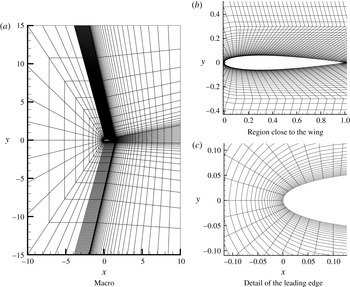
, a finer mesh with 4674 quadrilateral elements (shown in figure 2) was used to discretize the same domain, with an adaptive procedure employed to adjust the polynomial order between 2 and 11. The time step was
 $5\times 10^{-5}$
and the resolution in the span direction was fixed at 256 degrees of freedom per chord length, while the simulation time and spanwise length were different for each simulation, with values summarized in table 1. A longer span was used for the wavy wing with
 $\unicode[STIX]{x1D6FC}=15^{\circ }$
because flow visualizations from Paula (Reference Paula2016) suggest that the flow in this condition contains spanwise modes longer than two waviness wavelengths. In this case, it is still possible that a longer span would lead to different results, by allowing the existence of modes with longer spanwise wavelengths. However, this choice of span is consistent with other numerical studies available in the literature, where rarely more than four waviness wavelengths are considered. Both sets of simulations were stabilized using the spectral-vanishing viscosity technique (Kirby & Sherwin Reference Kirby and Sherwin2006b
), and the simulations with
 $Re=50\,000$
used the dealiasing technique described in Kirby & Sherwin (Reference Kirby and Sherwin2006a
) in the
 $xy$
plane, while for the Fourier expansion, the
 $3/2$
padding rule was used. More details on the parameters employed in the simulations can be found in Serson (Reference Serson2017).
The mesh used in the simulations with
 $Re=50\,000$
. Within each element, a
 $p$
th-order polynomial expansion is subsequently applied.

The parameters used in the simulations with
 $Re=50\,000$
.

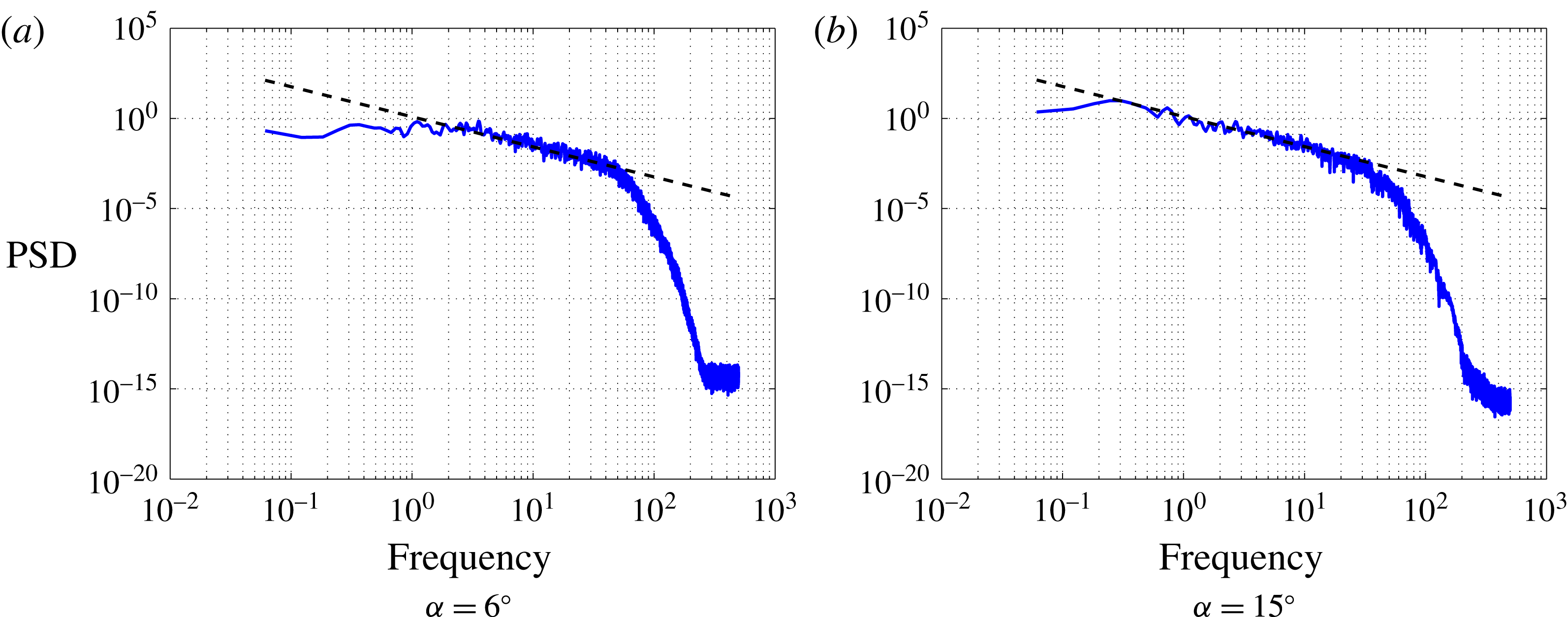
To illustrate how our simulations are able to resolve the small scales of the flow, figure 3 shows spectra of chordwise velocity fluctuations at a point with coordinates
 $(0.85,0.08,0.25)$
for simulations of the baseline wing with
 $Re=50\,000$
. By taking the
 $-5/3$
slope curve as a reference, we can clearly notice that the discretization employed in these simulations is capable of resolving flow scales well into the inertial range, and therefore should be capable of providing accurate results.
Spectra of
 $u$
-velocity fluctuations at the point
 $(0.85,0.08,0.25)$
for simulations of the baseline wing with
 $Re=50\,000$
. The dashed line corresponds to the
 $-5/3$
slope.

4 Results
We start by considering the effect of the waviness on the drag coefficient (
 $C_{D}$
) and lift coefficient (
 $C_{L}$
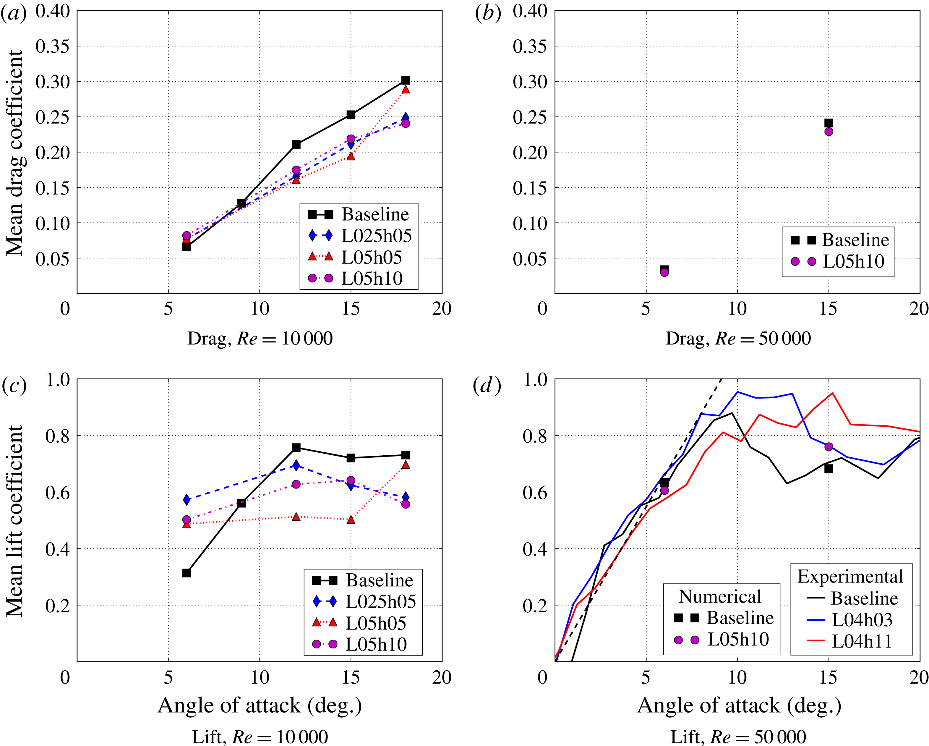
), with time-averaged results presented in figure 4. We notice that these results exhibit distinct behaviours. For
 $Re=10\,000$
, the waviness causes a large increase in
 $C_{L}$
at
 $\unicode[STIX]{x1D6FC}=6^{\circ }$
accompanied by a small increase in
 $C_{D}$
, resulting in a significant increase in the lift-to-drag ratio, while at the higher angles of attack, both lift and drag are significantly reduced, with the lift-to-drag ratio being similar for the baseline and wavy wings. On the other hand, for
 $Re=50\,000$
, there is little change for
 $\unicode[STIX]{x1D6FC}=6^{\circ }$
, with an increase in the lift and a decrease in the drag at
 $\unicode[STIX]{x1D6FC}=15^{\circ }$
. The
 $C_{L}$
results for
 $Re=50\,000$
are also compared with the experiments from Paula (Reference Paula2016), showing a good agreement. It should be noted that the geometry of our wavy wing is not the same as those from the experiments, but the observed effect of the waviness causing an increase in the lift is consistent with the experimental data.
Time-averaged drag and lift coefficients. For the lift with
 $Re=50\,000$
, the solid lines are experimental values from Paula (Reference Paula2016) and the dashed line is the
 $2\unicode[STIX]{x03C0}$
slope.

Comparison between the spectra of the lift coefficient for the baseline and L05h10 wings for different conditions.

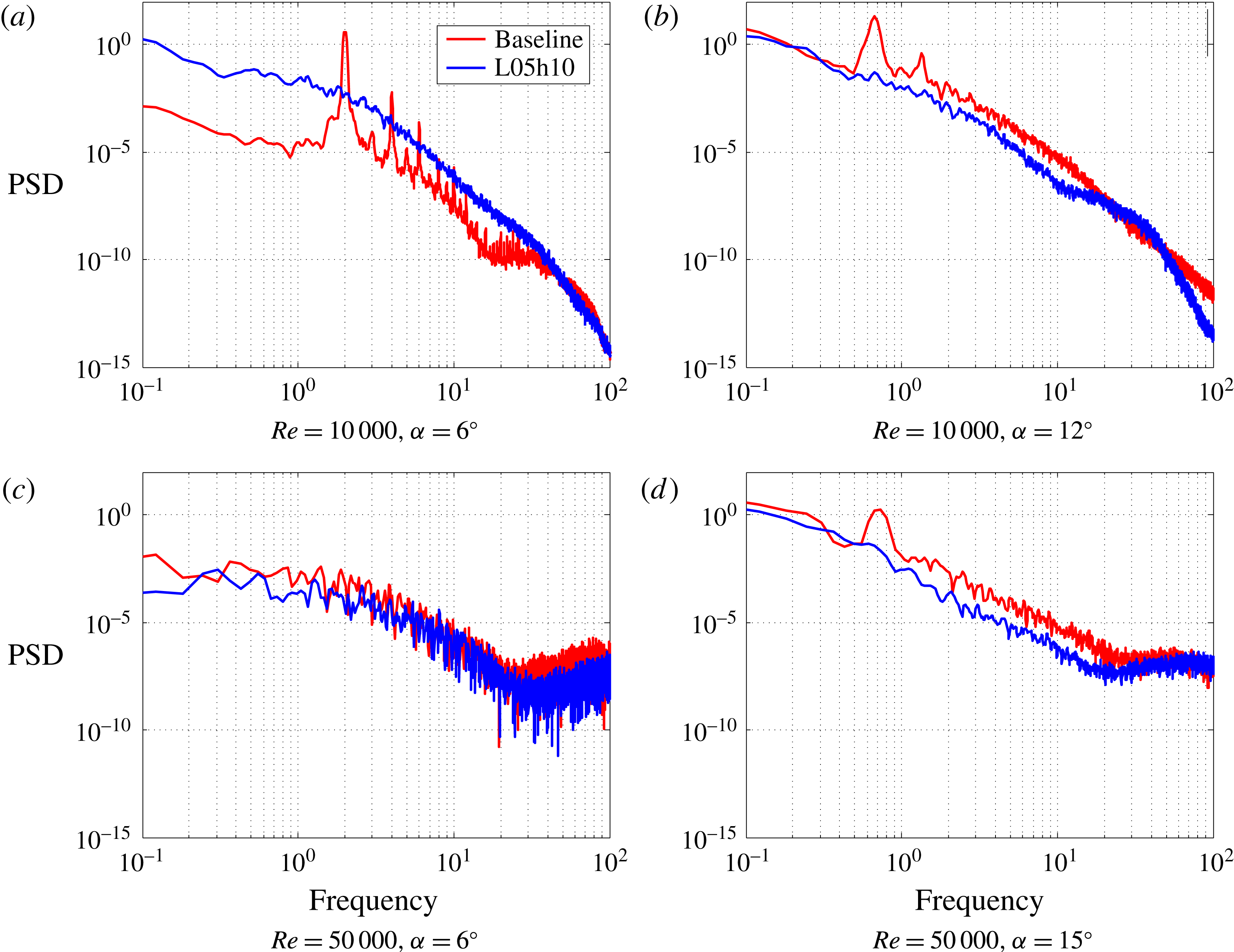
The effect of the waviness on the aerodynamic forces is not restricted to their time-averaged values, but also affects the qualitative characteristics of their time evolution. In order to analyse this behaviour, we consider the spectrum of the lift coefficient, represented by the power spectral density (PSD) as a function of the frequency in time. Figure 5 shows the spectra of the lift coefficient for different combinations of
 $Re$
and
 $\unicode[STIX]{x1D6FC}$
, comparing the results for the baseline and L05h10 wings. First, we note that the waviness suppresses the tonal component observed in the baseline wing, which can be associated with vortex shedding. Moreover, we note that for
 $Re=50\,000$
with
 $\unicode[STIX]{x1D6FC}=6^{\circ }$
, the spectra of both the baseline and the wavy wing present much lower intensity, indicating that the fluctuations are weaker in these cases compared with the rest of the simulations. Finally, for
 $Re=10\,000$
with
 $\unicode[STIX]{x1D6FC}=6^{\circ }$
, the baseline wing has a sharp peak around a Strouhal number of
 $St=2$
. The concentration of energy in a single frequency and its harmonics is typical of laminar flows, and flow visualizations confirm that this is indeed the case for the baseline wing, while the wavy wing is in a transitional regime. Therefore, the large increase in lift observed in this case is associated with the waviness inducing the transition of the flow, and consequently avoiding the loss of performance observed when the flow becomes completely laminar as the Reynolds number is decreased. This consideration is further supported by comparing the results with
 $\unicode[STIX]{x1D6FC}=6^{\circ }$
for the two different Reynolds numbers considered here and the results for
 $Re=1000$
from Serson et al. (Reference Serson, Meneghini and Sherwin2017). For
 $Re=1000$
, the flow is laminar for both the baseline wing and the wavy wing, with both presenting a low
 $C_{L}$
close to
 $0.3$
and the waviness having little impact on the aerodynamic forces. Similarly, for
 $Re=50\,000$
, the flow is transitional in both cases, and they both have
 $C_{L}$
around 0.6 (close to the
 $2\unicode[STIX]{x03C0}$
slope). The only case where the waviness has a significant impact on the lift at this angle of attack is for
 $Re=10\,000$
, where it pushes the
 $C_{L}$
from the laminar value of approximately
 $0.3$
towards the higher
 $Re$
value represented by the
 $2\unicode[STIX]{x03C0}$
slope.
Next, we consider the topology of the flow associated with the changes in
 $C_{L}$
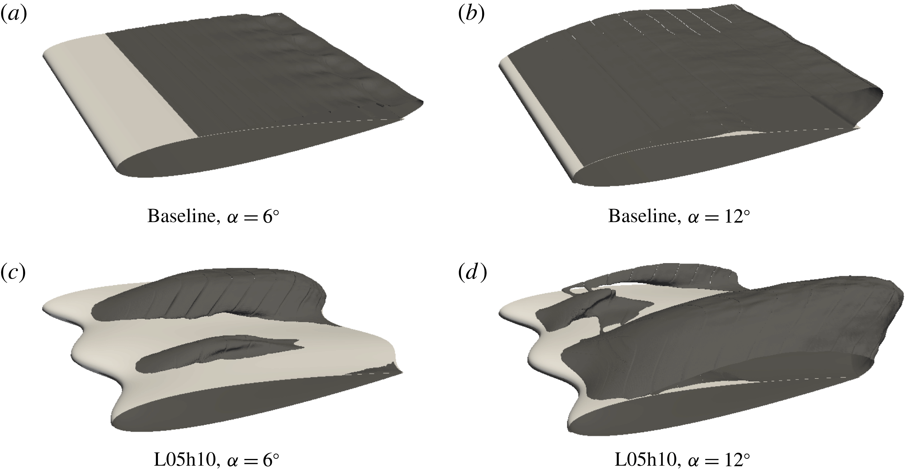
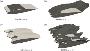
. Figures 6 and 7 show the time-averaged recirculation regions for simulations with
 $Re=10\,000$
and
 $Re=50\,000$
respectively. These are defined as the regions where the chordwise velocity becomes negative, and were obtained as isocontours of
 $u/U_{\infty }=-0.001$
. Although in some of the simulations the time-averaging interval may not be sufficient to converge to a true mean flow, the averaging serves the purpose of filtering high-frequency structures, allowing us to observe the main features of the flow. As expected, for the baseline wing, the flow is mostly two-dimensional, with widespread separation in all cases except for
 $Re=50\,000$
with
 $\unicode[STIX]{x1D6FC}=6^{\circ }$
, where we observe reattachment associated with the laminar separation bubble phenomenon. Introduction of the waviness leads to a tendency for the flow to remain attached behind the waviness peaks, with separation restricted to distinct regions behind the valleys. This is a pattern that is typically observed in the literature for this flow (Favier et al.
Reference Favier, Pinelli and Piomelli2012; Skillen et al.
Reference Skillen, Revell, Pinelli, Piomelli and Favier2015). We also note that, in most cases, the wavy wing shows a sub-harmonic behaviour, with the flow demonstrating notable variation along subsequent wavelengths of the waviness.
Time-averaged recirculation regions for simulations with
 $Re=10\,000$
.

Time-averaged recirculation regions for simulations with
 $Re=50\,000$
.

We next consider the pressure coefficient (
 $C_{p}$
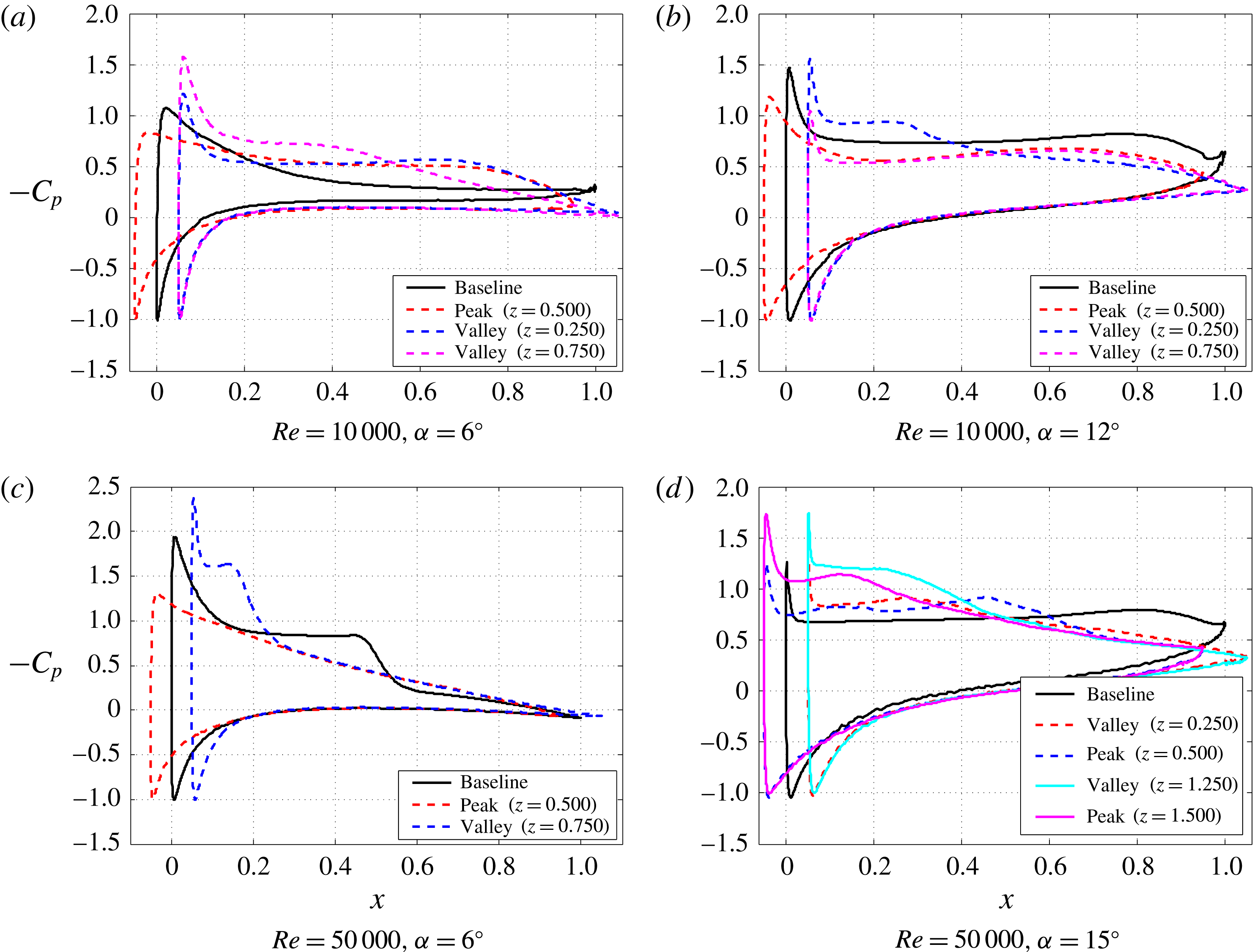
) distribution on the wing surface, since it is related to both the aerodynamic forces and the flow separation. The time-averaged curves for
 $-C_{p}$
are presented in figure 8. For each case, we present the result for the baseline wing as a reference, along with curves at different cross-sections of the modified wing. In some instances, more than one section corresponding to the waviness peak or valley are presented, due to the sub-harmonic behaviour of the flow. We note that although the waviness has little effect on the lift for
 $Re=50\,000$
with
 $\unicode[STIX]{x1D6FC}=6^{\circ }$
, the moment characteristics are quite distinct, which may be relevant in practical applications.
The time-averaged pressure coefficient distribution on the wing surface.

4.1 Flow around the leading edge
One characteristic feature of the
 $C_{p}$
distributions of figure 8 is that in general the peak section exhibits a lower suction peak when compared with the baseline wing. This behaviour is consistent with what we observed for lower
 $Re$
in Serson et al. (Reference Serson, Meneghini and Sherwin2017), and therefore we revisit those arguments to see whether the same physical mechanism is still important at these higher
 $Re$
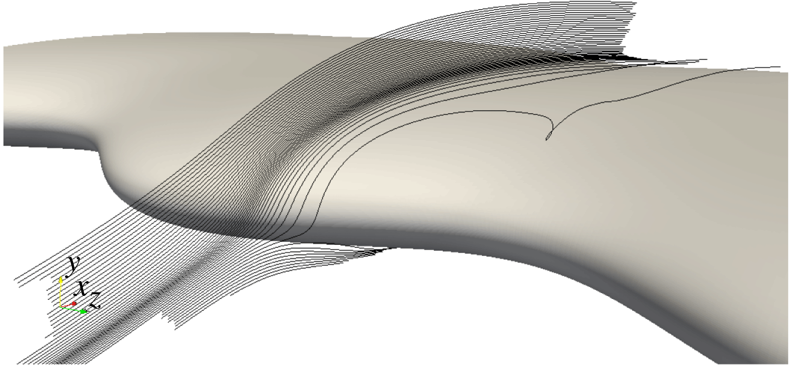
values. In that work, we argued that by extending the leading edge towards the incoming flow, spanwise pressure gradients are created which induce spanwise flow. Since the leading edge is located further upstream in the peak section compared with the troughs, the spanwise pressure gradient points towards the peaks in the lower portion of the wing (due to the high pressure of the stagnation point), while it points away from this section in the upper part of the wing (due to the low pressure of the suction peak). Therefore, this pressure gradient forces the flow to move away from the peak section in the lower portion of the wing, while fluid is drawn towards the suction peak of the peak section. In a more intuitive manner, this can be interpreted as the flow being deflected by the leading edge of the peak, and moving around it, as can be seen in the streamlines of figure 9. We note that these streamlines have similarities to those of Skillen et al. (Reference Skillen, Revell, Pinelli, Piomelli and Favier2015), who also observed a deflection of the flow by the wavy leading edge. Therefore, by deforming the leading edge, we create an alternative path, allowing part of the flow to circumvent the usual accelerating path around the leading edge in the
 $xy$
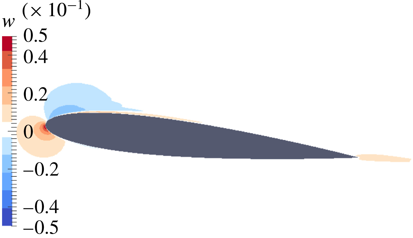
plane. Since this acceleration of the flow is responsible for generating the suction peak, the spanwise flow allowed by the deformation of the leading edge hinders the ability of the wing to generate a strong suction peak in the sections corresponding to the waviness peaks, contributing to weakening of the suction peak in these sections. The weaker suction peak then leads to weaker adverse pressure gradients, explaining why the flow remains attached in these sections. To determine whether this description is also valid in the present case, figure 10 shows contours of spanwise velocity at a cross-section positioned between a waviness peak and a trough. The peak is at
 $z=0$
and the trough is at
 $z=0.25$
, and therefore a positive velocity represents flow towards the trough. The figure clearly shows that the orientation of the spanwise flow is consistent with the previous discussion, and therefore we conclude that the same mechanism as proposed in Serson et al. (Reference Serson, Meneghini and Sherwin2017) for
 $Re=1000$
is still important even at a larger Reynolds number of
 $Re=50\,000$
. We also note that, downstream of the leading edge, there is a change in the orientation of the spanwise flow near the wing, with
 $w$
becoming positive in figure 10. This is consistent with the reversal in the spanwise pressure gradient observed in figure 8.
Streamlines for the average flow around the L05h10 wing with
 $\unicode[STIX]{x1D6FC}=6^{\circ }$
and
 $Re=50\,000$
. The seed points are located on a line parallel to the
 $y$
-axis with
 $x=-0.03$
and
 $z=0.6$
.

Time-averaged contours of spanwise velocity at
 $z=0.125$
for the L05h10 wing with
 $\unicode[STIX]{x1D6FC}=6^{\circ }$
and
 $Re=50\,000$
. Positive
 $z$
is pointing out of the page, towards the nearest trough.

The previous discussion relates the spanwise flow to the spanwise pressure gradient. To discard the possibility of this spanwise flow being caused by viscous stresses, figure 11 presents a slice of the contributions to the spanwise acceleration from the pressure gradient (
 $-\unicode[STIX]{x2202}p/\unicode[STIX]{x2202}z$
) and the viscous forces (
 $\unicode[STIX]{x1D708}\unicode[STIX]{x1D6FB}^{2}w$
) for the L05h10 wing with
 $\unicode[STIX]{x1D6FC}=6^{\circ }$
and
 $Re=50\,000$
. As expected, the viscous contribution is only relevant in a thin boundary layer. Moreover, in the leading edge region, which was the focus of the previous argument, the pressure force is one order of magnitude larger than the viscous component, and therefore is the most relevant effect.
Time-averaged contours of the pressure and viscous contributions to the spanwise acceleration at
 $z=0.125$
for the L05h10 wing with
 $\unicode[STIX]{x1D6FC}=6^{\circ }$
and
 $Re=50\,000$
. It should be noted that each plot uses a different scale.

The only simulation where a reduction in the suction peak was not observed in the peak section was with
 $Re=50\,000$
and
 $\unicode[STIX]{x1D6FC}=15^{\circ }$
, where the main differences in
 $C_{p}$
occur between the first two wavelengths and the second two wavelengths along the span instead of between peaks and troughs, which is consistent with the different extents of the separation regions shown in figure 7. To further our understanding of this phenomenon, we can consider, as a first approximation, that the effect from the tendency for weakening the suction peak is similar to what might be expected from a reduction in the angle of attack. In the pre-stall regime, or for much lower
 $Re$
where the lift coefficient curve is monotonic, this invariably leads to a decrease in the suction peak, accompanied by a reduction in
 $C_{L}$
. However, in the post-stall regime, it is possible that by attempting to reduce the suction peak, this mechanism causes the flow to reattach, as was observed for parts of the wavy wing in this case. Therefore, despite the tendency for the suction peak to be reduced, the overall effect in the post-stall regime is intricate since there are competing effects at play.
4.2 Effect of the waviness on transition
Returning now to figures 7 and 8(c), we also observe that for
 $Re=50\,000$
and
 $\unicode[STIX]{x1D6FC}=6^{\circ }$
, the separation bubble becomes shorter in the regions where the flow still separates. Since the reattachment of the laminar separation bubble is usually preceded by transition, this suggests that in the presence of the waviness, the flow transitions earlier in these sections compared with the baseline wing. Moreover, at this
 $Re$
, transition is not expected to occur in attached boundary layers, with the typical critical Reynolds number for a flat-plate boundary layer being of the order of
 $Re_{x,c}=3\times 10^{5}$
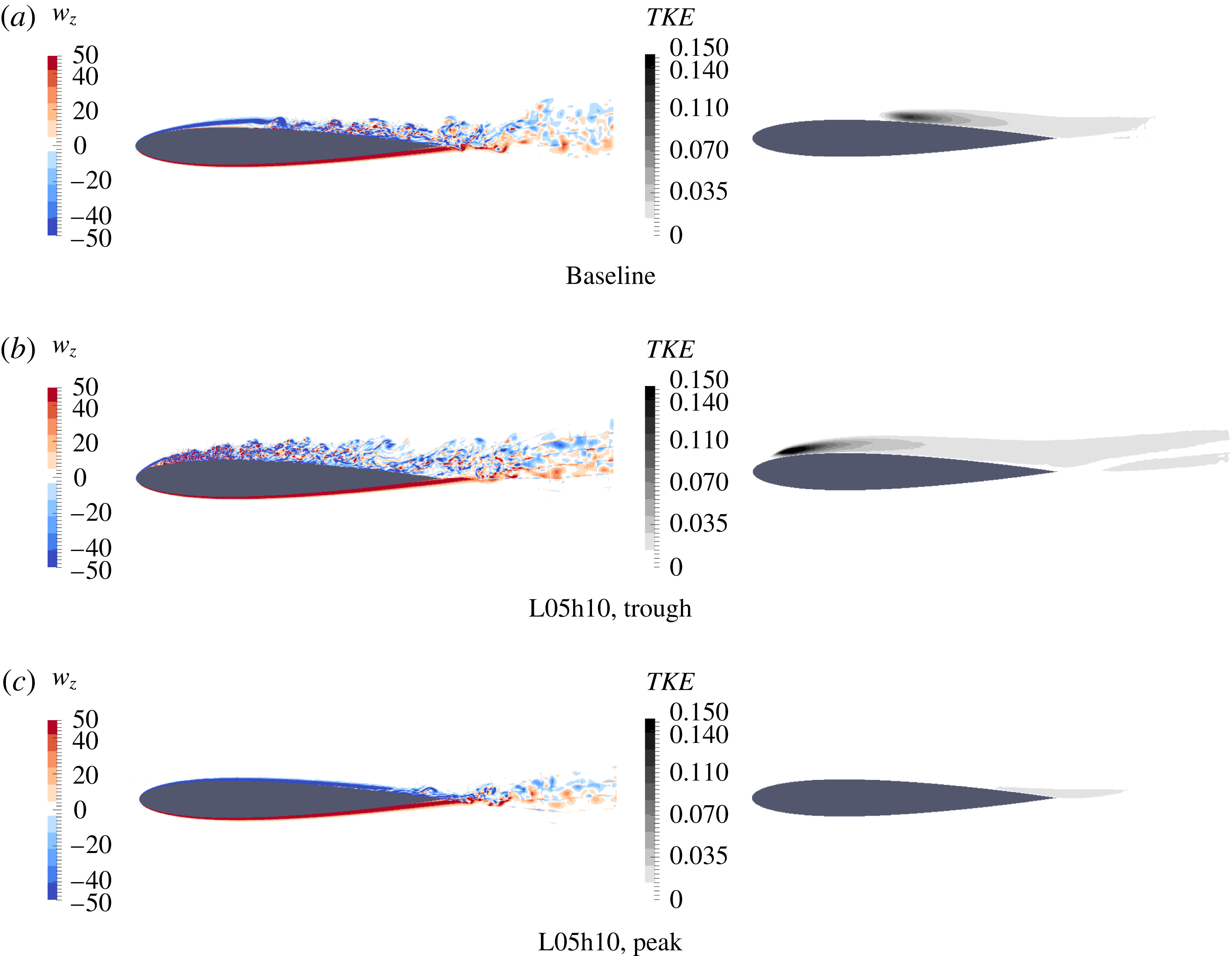
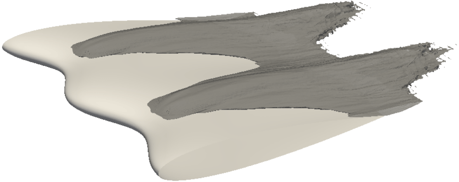
(McCormick Reference McCormick1995). Therefore, we expect the attached flow behind the peak sections of the wavy wing to be laminar. Figure 12 confirms these expectations by showing contours of spanwise vorticity and turbulence kinetic energy at different cross-sections. The transition point moves upstream in the trough section compared with the baseline, while transition is mostly suppressed in the peak section where the flow is attached. Although there is a small amount of turbulence in the peak section near the trailing edge, figure 13 illustrates how this is not generated at this location, but rather the turbulence from the trough section eventually propagates across the whole span.
Slices with contours of instantaneous spanwise vorticity (on the left) and of turbulence kinetic energy (
 $TKE$
) (on the right) for simulations with
 $\unicode[STIX]{x1D6FC}=6^{\circ }$
and
 $Re=50\,000$
.

The isosurface of
 $TKE=0.015$
for a wavy wing with
 $\unicode[STIX]{x1D6FC}=6^{\circ }$
and
 $Re=50\,000$
.

Considering the
 $C_{p}$
results for
 $Re=10\,000$
(figure 8
a,b), we note that the trough section with a larger separation region closely follows the pressure distribution from the peak section for most of the chord (starting at around
 $x=0.25$
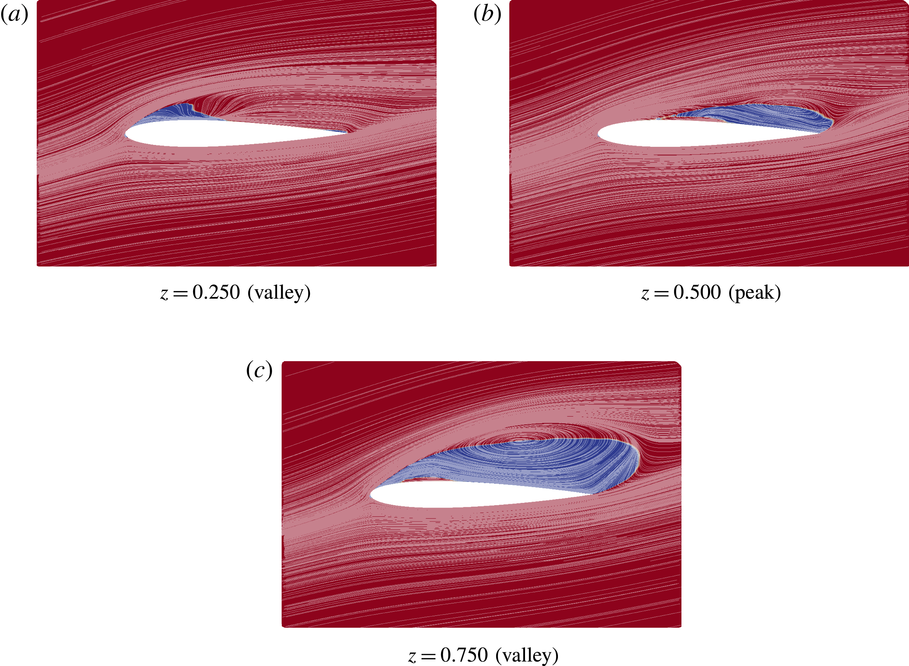
). The trough section with a smaller recirculation region, on the other hand, exhibits a low-pressure plateau, suggesting the presence of a laminar separation bubble with reattachment. The second peak section is not displayed in these figures because both peak sections have the same behaviour. Figure 14 shows streamlines projected onto the
 $xy$
plane for the same sections as those from the
 $C_{p}$
curves. For
 $z=0.25$
, there is a reattachment of the flow, which can be related to the pressure recovery observed in this section after the low-pressure plateau. On the other hand, the trough section at
 $z=0.75$
presents a fully separated flow.
Time-averaged streamlines projected onto the
 $xy$
planes at different sections for the L05h10 geometry with
 $\unicode[STIX]{x1D6FC}=12^{\circ }$
and
 $Re=10\,000$
. The colours represent the orientation of the chordwise velocity.

4.3 Low-frequency fluctuations
Another interesting behaviour is observed when we consider the time evolution of the lift coefficient for the simulations with
 $Re=50\,000$
and
 $\unicode[STIX]{x1D6FC}=15^{\circ }$
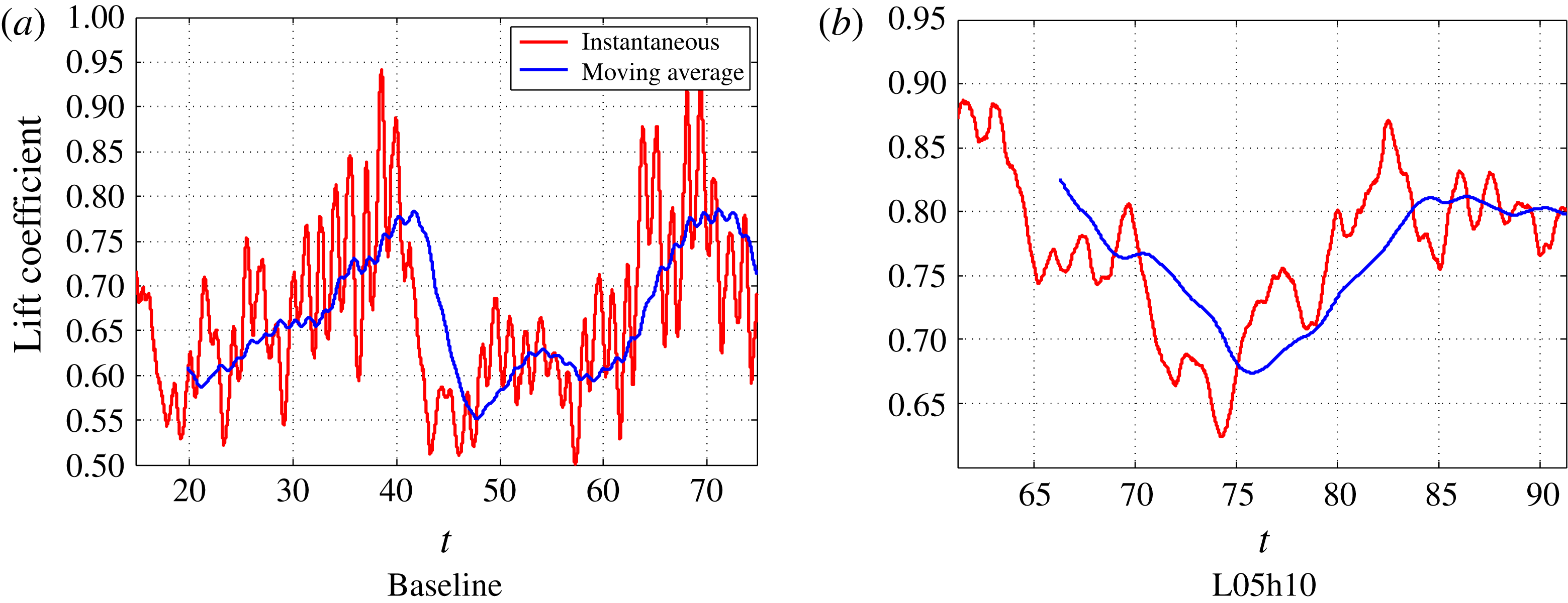
. Figure 15 shows how the instantaneous lift coefficient varies in time in these cases, and also a moving average with the aim of filtering all but the lowest frequencies of the result. We note that, for both geometries, there are significant low-frequency fluctuations, although they are quite different in each case. For the baseline wing, the
 $C_{L}$
tends to increase with time, until it undergoes a sharp drop. On the other hand, for the wavy wing, the flow slowly alternates between low- and high-lift configurations. Although the exact mechanisms for these behaviours are not known yet, in the following, we will provide some results that indicate possible explanations for them.
Instantaneous lift coefficient and moving average with a width of 5 time units for simulations with
 $Re=50\,000$
and
 $\unicode[STIX]{x1D6FC}=15^{\circ }$
.

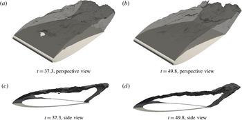
Recirculation region filtered using an exponential moving average with different final times for the baseline wing with
 $\unicode[STIX]{x1D6FC}=15^{\circ }$
and
 $Re=50\,000$
.

Considering first the baseline wing, we observed in figure 7 that the flow averaged over the entire
 $25$
time unit interval considered here is completely separated. However, this may not be the case for shorter periods of time. Figure 16 presents the recirculation region of the flow filtered using an exponential moving average with time constant
 $\unicode[STIX]{x1D70F}=1.5$
for different final times. This filter was used to remove the high-frequency turbulent fluctuations, while maintaining the distinctions that might explain the low-frequency behaviour. We observe that the recirculation isocontour of the high-lift configuration (
 $t=37.3$
) is broken near the centre of the span, while this does not happen in the low-lift case. This seems to be caused by an interaction with the secondary flow inside the separation bubble, which is present to different extents in both cases, as can be seen from the side view. Therefore, we can hypothesize that the lift initially increases as this secondary flow region grows and disturbs the separation bubble. This structure then bursts, leading to the sharp drop in the
 $C_{L}$
observed in figure 15(a) at around
 $t=40$
.
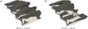
Following an analogous approach to that of the baseline case, figure 17 presents recirculation regions of the flow average over different intervals for the wavy wing. This figure shows a significant distinction between the two intervals in the second half of the span (
 $1<z<2$
). In this region, separation is much more extensive in the lower-
 $C_{L}$
configuration, while in the higher-
 $C_{L}$
configuration, there is flow reattachment in most of this region. Therefore, we associate the changes in separation patterns in some portions of the span as being responsible for the low-frequency variation of the lift.
Recirculation regions for flow obtained using different time-averaging intervals for the wavy wing with
 $\unicode[STIX]{x1D6FC}=15^{\circ }$
and
 $Re=50\,000$
.

5 Conclusions
We have presented a numerical study on the effect of spanwise waviness on the flow around infinite wings. This was accomplished through highly resolved direct numerical simulations, considering
 $Re=10\,000$
and
 $Re=50\,000$
at different angles of attack in both the pre-stall and post-stall regimes. Our results show that, depending on the Reynolds number and angle of attack, the waviness can either increase or decrease the lift coefficient. In particular, for
 $Re=10\,000$
, the waviness greatly increases
 $C_{L}$
for
 $\unicode[STIX]{x1D6FC}=6^{\circ }$
and reduces it for higher angles of attack, while for
 $Re=50\,000$
, there is little impact for
 $\unicode[STIX]{x1D6FC}=6^{\circ }$
and
 $C_{L}$
is increased for
 $\unicode[STIX]{x1D6FC}=15^{\circ }$
.
The flow visualizations show a tendency for separation to be restricted to regions behind the waviness troughs, with the flow remaining attached behind the peaks, which is consistent with results from the literature (Favier et al.
Reference Favier, Pinelli and Piomelli2012; Skillen et al.
Reference Skillen, Revell, Pinelli, Piomelli and Favier2015). Moreover, they show a significant sub-harmonic behaviour, similar to what was observed numerically by Rostamzadeh et al. (Reference Rostamzadeh, Hansen, Kelso and Dally2014) and experimentally by Paula (Reference Paula2016). For example, at
 $Re=10\,000$
, one of the trough sections exhibits a laminar separation bubble phenomenon with reattachment of the flow, while the flow is fully separated in the other trough section.
In terms of the physical mechanisms involved in this flow, we have shown that the weakening of the suction peak in the sections of peak waviness plays an important role in explaining the separation patterns of this flow. By deforming the leading edge, we allow for spanwise flow, which hinders the ability of the wing to force the flow to accelerate around the leading edge, leading to weaker suctions on the sections behind the waviness peaks. This mechanism had previously been proposed at a much lower Reynolds number of
 $Re=1000$
(Serson et al.
Reference Serson, Meneghini and Sherwin2017), and we showed that it remains important even at
 $Re=50\,000$
. Although this is not the only way in which the waviness affects the flow, it seems to be an important mechanism that is present in a wide range of
 $Re$
, and therefore any attempt to explain how the waviness acts should consider it. In some of our simulations (e.g.
 $Re=50\,000$
with
 $\unicode[STIX]{x1D6FC}=6^{\circ }$
), we can also observe an improved suction peak behind the troughs, which is also likely to have a significant impact on the aerodynamic forces. This is similar to what was observed by Skillen et al. (Reference Skillen, Revell, Pinelli, Piomelli and Favier2015), who proposed that this is caused by the acceleration of the flow deflected by the leading edge towards these regions. However, this effect is not obtained as consistently as the weakening of the suction peak behind the peak sections, being observed only in some situations. For example, it is not present for
 $Re=10\,000$
with
 $\unicode[STIX]{x1D6FC}=12^{\circ }$
, and the simulations with
 $Re=1000$
from Serson et al. (Reference Serson, Meneghini and Sherwin2017) exhibit a weakening of the suction peaks behind the troughs.
Another effect we observe in this range of Reynolds number is that the separated shear layers tend to transition earlier in the presence of the waviness. For
 $Re=10\,000$
and
 $\unicode[STIX]{x1D6FC}=6^{\circ }$
, the flow around the baseline wing is completely laminar, while for the wavy wing, we have a transitional flow. This explains the significant increase of
 $C_{L}$
in this case, and therefore we can conclude that the waviness offers the advantage of delaying the loss of lift observed as the Reynolds number is decreased, since, in the presence of the waviness, the flow becomes completely laminar at lower
 $Re$
than for the baseline wing. This earlier transition was also observed for
 $Re=50\,000$
, where it led to a shorter laminar separation bubble at
 $\unicode[STIX]{x1D6FC}=6^{\circ }$
due to the earlier transition.
Acknowledgements
D.S. and J.R.M. are grateful for the support received from CNPq (grants 231787/2013-8 and 312755/2014-7) and FAPESP (grants 2012/23493-0 and 2014/50279-4). S.J.S. would like to acknowledge support under the Royal Academy of Engineering Research Chair Scheme (no. 10145/86) and support under EPSRC grant EP/K037536/1. The simulations were performed on the Archer National Supercomputer using allocation provided by the UK Turbulence Consortium (EPSRC grant EP/L000261/1). Data supporting this publication can be obtained on request from nektar-users@imperial.ac.uk.