Design and methodology

The microstrip patch antenna utilized in this work was designed using an FR-4 substrate because of its desirable electrical characteristics, low expense of manufacture, and simple fabrication. The antenna is made up of a copper ground plane and patch, with the FR-4 substrate between them. The patch size and substrate thickness were optimized using iterative design simulations in CST Studio to obtain an operating frequency of 4.2 GHz. The antenna was optimized using a circular patch structure, which was selected for its compact size and good performance. Various iterations were done to optimize the impedance matching of the antenna for maximizing its radiation efficiency. The design process of micro-strip patch antennas requires consideration of several important parameters, which include substrate dielectric constant ( ${\varepsilon _r}$), target operating frequency ( $f$), and the substrate thickness ( $h$). Both dimensions of the patch and the substrate get defined through the application of these established factors. The required dimensions of the patch require empirical equations that calculate length ( $L$) and width ( $W$) from desired resonant frequency and dielectric constant data. The substrate material wavelength ( $\lambda $) determines the typical length of the patch design ( $L$) when divided by 2. The width of the antenna ( $W$) can be determined through impedance matching measurements, while bandwidth plays a major role in defining this measurement. The antenna design requires knowledge of both the effective dielectric constant and the operating mode of the antenna for the mathematical calculations. The substrate’s thickness selection ( $h$) follows both dielectric material specifications and design requirements.

The front and back views of the final design for the proposed MPSMA are shown in Fig. 1(a). The front view displays a pentagon slotted circular patch, which includes patch diameter (P _R), feed length (F _L), feed width (F _W) as well as substrate width (S _W) and substrate length (S _L). A detailed depiction in the back view displays the ground plane where it shows both the ground width (G _W) and ground length (G _L). The design merged the features of pentagonal slots and triangular slots embedded in a circular patch to enhance impedance matching and enhance radiation effectiveness while reducing the return loss, which is suitable for biomedical sensing operations.

Figure 1.

(a) Proposed MPSMA design. (b) Iteration of the proposed MPSMA design. (c) S₁₁ comparison of various patch iterations of the proposed MPSMA. (d) Proposed MPSMA ground plane iteration. (e) S₁₁ comparison of various ground length (GL) iterations.

Figure 1 Long description

The image A showing two rectangular diagrams labeled Front View and Back View. The Front View diagram shows a circular patch with multiple internal slot shapes and a feed line extending downward. Dimension labels shown include S subscript w across the top, S subscript l along the left side, P subscript r along the right side, F subscript l along the left of the feed and F subscript w across the feed width. The Back View diagram shows a rectangle with a horizontal division near the bottom and dimension labels G subscript l along the left side and G subscript w along the bottom. The image B showing six patch-shape iterations arranged in two rows of three, with arrows between shapes indicating a sequence. Each shape includes a circular or polygonal patch area and a vertical feed section. The image C showing a line graph with the horizontal axis labeled Frequency parentheses gigahertz right parenthesis and the vertical axis labeled S subscript 11 parentheses decibel right parenthesis. The frequency axis runs from 0 to 6. The S subscript 11 axis runs from 0 to negative 40. A legend lists Iteration 1, Iteration 2, Iteration 3, Iteration 4, Iteration 5 and Iteration 6. All curves dip to a minimum near about 3 on the frequency axis, reaching around negative 35 to negative 40 on the S subscript 11 axis, then rise toward higher frequencies. The image D showing four rectangular blocks in a left-to-right sequence with arrows between them. The first block has dimension labels 20 millimeter on the left side and 18 millimeter along the bottom. The second block has a label 16 millimeter near the left side. The third block has a label 10 millimeter near the left side. The fourth block has a label 4 millimeter near the left side. The image E showing a line graph with the horizontal axis labeled Frequency parentheses gigahertz right parenthesis and the vertical axis labeled S subscript 11 parentheses decibel right parenthesis. The frequency axis runs from 0 to 6. The S subscript 11 axis runs from 0 to negative 40. The legend lists G subscript l equals 4 millimeter, G subscript l equals 6 millimeter, G subscript l equals 8 millimeter, G subscript l equals 10 millimeter and G subscript l equals 12 millimeter. One curve shows a deep minimum near about 3 on the frequency axis reaching close to negative 40, while the other curves remain closer to 0 to negative 10 across most of the frequency range with smaller dips.

The optimized patch design undergoes six design rounds whose dimensions are highlighted in Table 1. The parameters consisting of circular patch diameter, pentagon side length, and slot shape dimensions underwent modifications during six optimization rounds depicted in Fig. 1(b) to enhance return loss performance and bandwidth while achieving proper impedance matching. The selected dimensions of substrate matched with enough clearance to ground, while the patch area was modified for specific resonance characteristics and dielectric requirements. The optimized design succeeds in integrating all essential aspects of gain, radiation efficiency, and return loss, which suit applications in glucose sensing effectively.

Table 1.

Dimensions of proposed MPSMA

Table 1 Long description

The table lists eight labeled parameters and their dimensions in millimeters for a proposed design. SL is 20 millimeters, the largest value, while SW and GW are both 18 millimeters. PL is 10 millimeters and PW is 8 millimeters, placing them in the mid range. Smaller measurements include FL at 5 millimeters, GL at 4 millimeters, and FW at 3 millimeters, the smallest value. Overall, most dimensions cluster between 3 and 20 millimeters, with two parameters sharing the same 18 millimeter value. The parameter labels are abbreviations and are not defined in the table, so their physical meaning cannot be inferred from the data alone.

The systematic design process of the proposed MPSMA through six sequential patch iterations is shown in Fig. 1(b). The antenna design commences with a circular patch followed by the placement of a pentagonal slot at its center area to enhance resonant characteristics. Symmetric cuts along with slots are progressively added to optimize impedance matching and enhance return loss as depicted in Fig. 1(c).

The optimized results were achieved by making iterations in the ground length (G _L), as shown in Fig. 1(d). Initially, a full ground plane was kept for the design and further the length was reduced by a trial-and-error method. The optimized antenna ground plane (G _L = 4 mm) achieves optimal signal transmission while boosting antenna performance during its final iteration of development. The final design of the antenna obtained a return loss (S₁₁) of −36.36 dB at frequency (F = 4.2 GHz), which is depicted in Fig. 1(e). An equivalent circuit is proposed for the antenna in Fig. 2(a). The designed antenna is modeled by a parallel RLC circuit with value of resistance R = 49 ohms, C = 0.7 pF, and L = 2.1 nH. The antenna offers maximum current flow through the patch at the parallel resonance frequency (4.2 GHz) due to minimum impedance offered. It is observed that the reflection characteristics of the proposed antenna by equivalent circuit modeling and full-wave simulations bear close resemblance.

Figure 2.

(a) Comparison between reflection characteristics of the proposed antenna by equivalent circuit modeling and full-wave simulations. (b) Fabricated MPSMA. (c) Comparison of the tested vs simulated S₁₁. (d) Comparison of the tested vs simulated VSWR.

Figure 2 Long description

Panel (a) shows a line graph comparing reflection characteristics using ADS and CST models. The x-axis is Frequency (gigahertz) from 2 to 8 and the y-axis is S subscript 11 (decibel) from 0 to minus 40. The ADS curve shows a dip near 4.2 gigahertz at approximately minus 36 decibels. Panel (b) displays front and back views of the fabricated MPSMA next to a coin for scale. Panel (c) includes two line graphs. The first graph shows Tested S11 with a dip at 4.2 gigahertz reaching minus 36 decibels. The second graph shows Simulated S11 with a similar dip. Panel (d) presents two line graphs for VSWR. The first graph shows Tested VSWR with a minimum near 4.2 gigahertz. The second graph shows Simulated VSWR with a similar pattern. The graphs demonstrate close agreement between tested and simulated data, with minor offsets. Curves are distinguished by dashed and solid lines.

MPSMA simulated and tested results

The fabrication of the proposed MPSMA was completed using selected FR-4 as the substrate material, which is shown in Fig. 2(b), as it exhibits a dielectric constant of 4.3 and a thickness of 1.6 mm, suitable for the fabrication process. The main reason for choosing the abovementioned substrate is ease of availability and cost. The fabricated antenna was measured using a Vector Network Analyzer (VNA) in an anechoic chamber, and the obtained results closely agreed with the simulation outcomes. The testing results prove that this antenna provides flawless performance for glucose sensing applications due to its outstanding return loss, together with low VSWR and high gain and efficiency as shown in Table 2. The simulated antenna exhibited a resonant frequency at 4.20 GHz with an S₁₁ of −36.36 dB, while the measured result showed a resonance at 4.91 GHz with an S₁₁ of −33.19 dB. This corresponds to a frequency deviation of approximately 16.90%, which can be attributed to fabrication tolerances, material inconsistencies, and measurement setup imperfections. Despite the shift, both results indicate excellent impedance matching, with return losses well below −30 dB as shown in Fig. 2(c). The simulated VSWR value at resonance is 1.03, while the measured VSWR is 1.1, indicating a 6.80% deviation as shown in Fig. 2(d). This minor variation may result from measurement noise, fabrication tolerance, or connector losses. Both values are close to 1, confirming a very good impedance matching.

Table 2.

Comparison of the tested vs simulated VSWR

Table 2 Long description

The table compares simulated and measured antenna performance metrics: return loss, resonant frequency, gain, VSWR, and efficiency. Return loss is slightly less negative in measurement at minus 33.19 decibels than in simulation at minus 36.36 decibels. Resonant frequency shifts upward from 4.2 gigahertz in simulation to 4.91 gigahertz in measurement. Gain increases from 1.47 dBi in simulation to 2.251 dBi in measurement. VSWR remains close between the two, changing from 1.03 simulated to 1.1 measured. Efficiency is listed as 72.12 percent for simulation, but the measurement value is not available, so efficiency cannot be compared.

Glucose detection using multilayer finger model

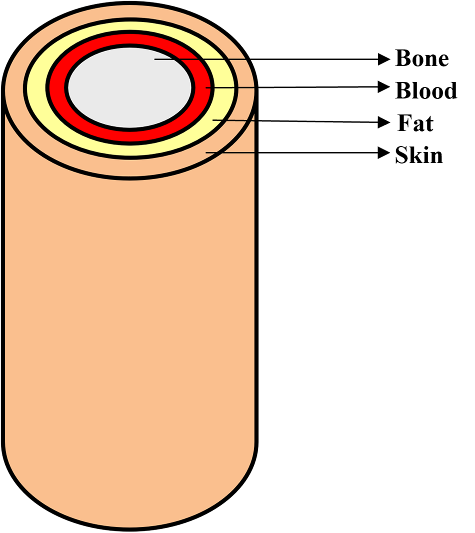
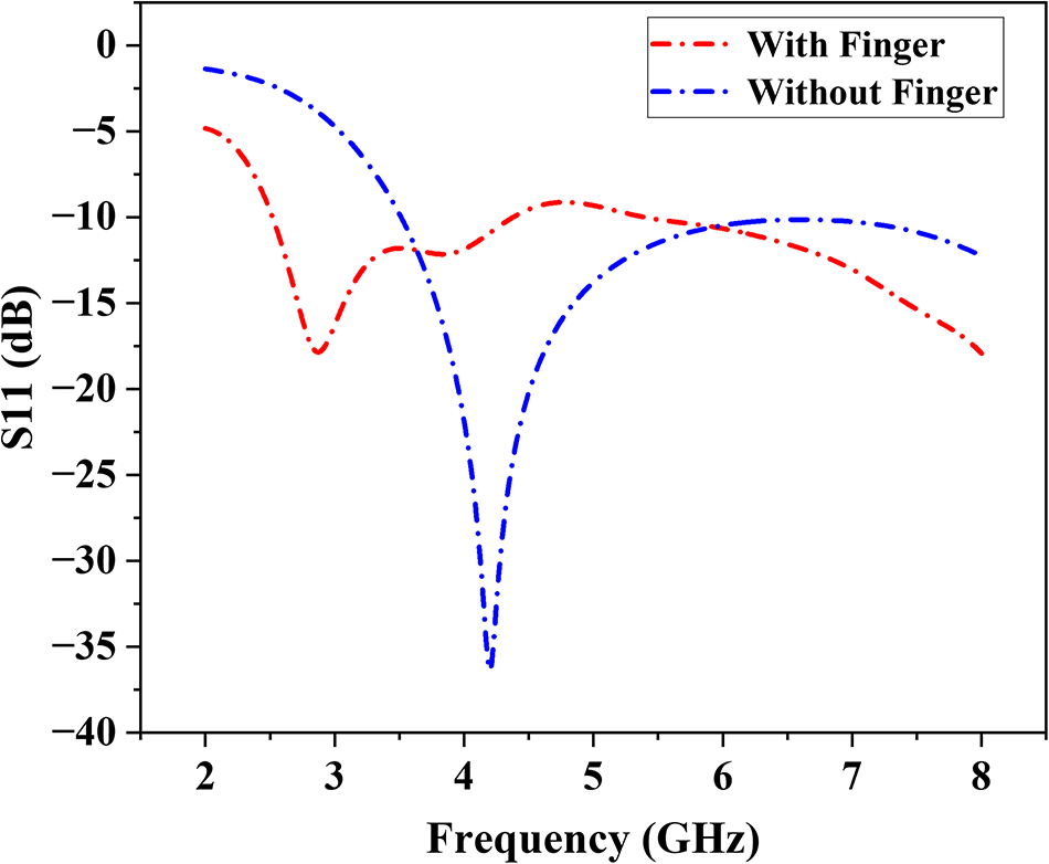
In order to proceed with blood glucose detection, a multilayer finger model is developed followed by antenna design for biologically similar human tissue structure simulation as shown in Fig. 3. The designed finger model contains four layers starting from skin and continuing into fat and blood, and ending with bone deep inside as shown in Fig. 4. Each layer represents distinct electrical characteristics together with structural characteristics of real human tissue. The properties considered for the creation of each layer are listed in Table 3. Initially, simulations were carried out using the proposed MPSMA alone, and later, the proposed antenna was simulated against a multilayer finger model. The S₁₁ comparison between both simulations was depicted in Fig. 5. An adequate frequency shift and variation in S₁₁ were observed with and without the finger simulation. The fundamental idea behind non-invasive glucose sensing is to identify even the smallest shift in human blood permittivity brought on by variations in glucose concentration. It suggests that the blood’s complex permittivity depends on the amount of glucose present. This is the primary factor that we need to take into account when doing any EM modeling pertaining to blood glucose sensing.

Figure 3.

Block diagram for multilayer finger model simulation setup.

Figure 4.

Multilayer finger model.

Figure 5.

S₁₁ comparison with and without the finger model.

Table 3.

Comparison of physical properties for the human finger model

Table 3 Long description

The table lists four layers in a human finger model and compares their thickness, electrical permittivity, electrical conductivity, and density. Bone is the thickest layer at 8 mm and also has the highest density at 1908 kg per cubic meter. Skin is 2 mm thick but has the highest permittivity at 36.423, much higher than bone, blood, or fat. Bone has the highest conductivity at 10.429, while fat has the lowest conductivity at 0.536. Blood is 3.5 mm thick with permittivity 5.530 and conductivity 5.530, and its density is 1050 kg per cubic meter. Overall, thickness does not track with permittivity, since the thinnest layer has the highest permittivity. Values are presented as single numbers per layer with no units given for permittivity or conductivity, so measurement conditions and frequency are not specified.

According to the Cole–Cole model used in the simulation, the frequency-dependent complex permittivity of blood can be represented by equation (1), where ${\sigma _i}\,$ is the conductivity and $\alpha $ is the angular frequency, ${\varepsilon _\infty }$ is the high-frequency permittivity, $\Delta {\varepsilon _n}\,$ is the magnitude of the dispersion, and ${\tau _n}$ is the relaxation time constant.

(1)\begin{equation}\widehat\varepsilon(\omega)=\varepsilon_\infty+\sum_n\frac{\Delta\varepsilon_n}{1+(j\omega\tau_n)^{(1-\alpha_n)}}+\frac{\sigma_i}{j\omega\varepsilon_0}\end{equation}

The different glucose levels (0–16,000 mg) are attained by changing the electrical properties of the blood model (Cole–Cole model) [Reference Jeyakumar, Vishwa and Yuvaprabha25]. The simulations were carried out by placing the proposed MPSMA against the finger model. Multiple simulations were conducted using different blood models to mimic various glucose concentrations. A total of eight simulations were performed using different thumb BGLs, ranging from 0 mg/dL to 16,000 mg/dL. Figure 6(a) displays the reflection coefficient plot for every glucose concentration scenario. The plot illustrates how the resonance frequency of the suggested sensor varies with varying glucose concentration levels.

Figure 6.

(a) Frequency vs S₁₁ response for various blood glucose concentrations. (b) PCA of S₁₁ vs glucose concentration. (c) 2D scatter plot (PC1 vs PC2). (d) Various positions of the finger model placement.

Figure 6 Long description

The image A showing a line graph with the horizontal axis labeled Frequency gigahertz, ranging from 2 to 9. The vertical axis is labeled S11 decibel, ranging from negative 18 to 0. A legend lists 0 milligram, 250 milligram, 500 milligram, 1000 milligram, 2000 milligram, 4000 milligram, 8000 milligram and 16000 milligram. Multiple lines follow a similar path: near 2 gigahertz the curves are close to about negative 2 to negative 4 decibel, then drop to a minimum near about 2.7 gigahertz at about negative 16 to negative 18 decibel, rise to around negative 6 to negative 8 decibel near about 3.6 gigahertz, dip again near about 4.2 gigahertz to around negative 10 to negative 12 decibel, then rise toward about negative 6 to negative 8 decibel near about 5 gigahertz and then trend downward toward about negative 16 to negative 18 decibel by about 8.5 to 9 gigahertz. The image B showing a scatter plot titled PCA Results for Reflection Coefficient for Various Glucose Concentrations in Blood Model. The horizontal axis is labeled Principal Component 1, ranging from negative 60 to 60. The vertical axis is labeled Principal Component 2, ranging from negative 60 to 60. Points are plotted with labels including 0 milligram, 250 milligram, 500 milligram, 1000 milligram, 2000 milligram, 4000 milligram, 8000 milligram and 16000 milligram. Visible labeled points include approximately left parenthesis negative 50, 0 right parenthesis for 0 milligram, left parenthesis negative 50, negative 30 right parenthesis for 250 milligram, left parenthesis 50, 0 right parenthesis for 16000 milligram and several points clustered in the upper right quadrant around Principal Component 1 from about 35 to 55 and Principal Component 2 from about 25 to 45. The image C showing a scatter plot titled 2D PCA Scatter Plot PC1 vs PC2. The horizontal axis is labeled Principal Component 1, ranging from about negative 0.6 to 0.6. The vertical axis is labeled Principal Component 2, ranging from about negative 0.4 to 0.5. A continuous sequence of points forms a curved path starting near about left parenthesis negative 0.55, 0.45 right parenthesis, moving downward and right to around left parenthesis negative 0.25, negative 0.35 right parenthesis, then curving upward toward around left parenthesis 0.15, negative 0.05 right parenthesis and extending to the right toward about left parenthesis 0.55, 0.35 right parenthesis. A vertical color scale bar appears to the right of the plot. The image D showing five separate antenna diagrams in a row. Each diagram has a label Antenna above it and a numeric label below it: negative 1, negative 0.5, 0, 0.5 and 1. Each diagram shows concentric circular ring shapes centered within a square outline, with a horizontal line segment below the square.

The measured S₁₁ and frequency responses for different glucose concentrations show small but noticeable changes, as depicted in Table 4. The S₁₁ stays stable at around −17.8 dB, but frequency shifts toward higher values at higher glucose levels (especially 2000 and 8000 mg), which is what we would expect because of dielectric variation. These results show that it is possible to use microwave-based sensors to keep an eye on glucose levels.

Table 4.

Comparison of frequency vs S₁₁ for various blood glucose concentrations

Table 4 Long description

The table lists glucose concentration in milligrams alongside measured S11 in decibels and the corresponding frequency in gigahertz. Across all concentrations, S11 varies only slightly, ranging from about minus 17.47 dB to minus 17.85 dB. The least negative S11, about minus 17.47 dB, occurs at 2000 mg, and another relatively high value, about minus 17.50 dB, occurs at 8000 mg. Most other concentrations cluster near minus 17.82 to minus 17.85 dB, including 0 mg and 16000 mg at about minus 17.85 dB. Frequency is usually 2.870 GHz at 0, 500, 1000, 4000, and 8000 mg, with small shifts to 2.890 GHz at 250 mg, 2.882 GHz at 16000 mg, and the highest value of about 2.912 GHz at 2000 and 8000 mg. Overall, the data suggest minimal change in S11 and only minor frequency shifts across the tested glucose range. Because no uncertainty, repeats, or measurement conditions are provided, the small differences should be interpreted cautiously.

The S₁₁ vs frequency data analysis requires PCA for identifying distinct characteristics between various glucose concentrations. The dataset was initially normalized to ensure PCA is not biased by scale. It is observed that the dataset is highly collinear, which means the changes across different concentrations are strongly correlated. Figure 6(b) shows different glucose concentrations (0–16,000 mg) projected onto the first two principal components, and Fig. 6(c) shows how the PCA-transformed data points vary with frequency across all glucose levels.

Analysis of MPSMA against the finger model in various locations

The effectiveness of glucose concentration detection is confirmed by shifting the finger in different lateral positions as shown in Fig. 6(d). The various lateral positions are from −1 to +1 scale values. The different layers in the simulation possess separate permittivity together with different conductance and density values. The different shift scenarios help in reliable system performance even when the finger positions are not perfect. This observation is very important because finger movement is common during real-world biomedical sensing applications.

The simulation results indicate a stable response when shifted in different lateral directions, which enhances its resistance to change and optimizes detection accuracy through the finger model. Table 5 shows the S₁₁ vs frequency response for various shifts concerning 0 mg, 500 mg, 2000 mg, and 8000 mg glucose concentration and its corresponding graphical representation is shown in Fig. 7. The antenna maintains a reliable signal quality across different placement positions because the S₁₁ values remain consistently stable. The resonant frequency increases as glucose concentration rises because blood dielectric properties directly impact how the antenna responds, which proves its potential to monitor glucose levels without invasive procedures.

Figure 7.

S₁₁ vs frequency for shifting of finger position (a) 0 mg, (b) 500 mg, (c) 2000 mg, and (d) 8000 mg.

Figure 7 Long description

The image A showing a line graph titled 0mg. A legend lists: No Shift, minus 0.5 millimeter Left, minus 1 millimeter Left, plus 0.5 millimeter Right, plus 1 millimeter Right. The x-axis is labeled Frequency(GHz), ranging from 2 to 8 with tick marks at 2, 3, 4, 5, 6, 7, 8. The y-axis is labeled S11(dB), ranging from minus 20 to minus 4 with tick marks at minus 20, minus 18, minus 16, minus 14, minus 12, minus 10, minus 8, minus 6, minus 4. The plotted curves overlap closely. The curve is near minus 5 at about 2 gigahertz, drops to about minus 18 near 3 gigahertz, rises to about minus 12 near 3.5 gigahertz, rises further to about minus 9 near 5 gigahertz, then declines to about minus 18 near 8 gigahertz. The image B showing a line graph titled 500mg. A legend lists: No Shift, minus 0.5 millimeter Left, minus 1 millimeter Left, plus 0.5 millimeter Right, plus 1 millimeter Right. The x-axis is labeled Frequency(GHz), ranging from 2 to 8 with tick marks at 2, 3, 4, 5, 6, 7, 8. The y-axis is labeled S11(dB), ranging from minus 20 to minus 4 with tick marks at minus 20, minus 18, minus 16, minus 14, minus 12, minus 10, minus 8, minus 6, minus 4. The plotted curves overlap closely. The curve is near minus 5 at about 2 gigahertz, drops to about minus 18 near 3 gigahertz, rises to about minus 12 near 3.5 gigahertz, rises to about minus 9 near 5 gigahertz, then declines to about minus 18 near 8 gigahertz. The image C showing a line graph titled 2000mg. A legend lists: No Shift, minus 0.5 millimeter Left, minus 1 millimeter Left, plus 0.5 millimeter Right, plus 1 millimeter Right. The x-axis is labeled Frequency(GHz), ranging from 2 to 8 with tick marks at 2, 3, 4, 5, 6, 7, 8. The y-axis is labeled S11(dB), ranging from minus 20 to minus 4 with tick marks at minus 20, minus 18, minus 16, minus 14, minus 12, minus 10, minus 8, minus 6, minus 4. The plotted curves overlap closely. The curve is near minus 5 at about 2 gigahertz, drops to about minus 18 near 3 gigahertz, rises to about minus 12 near 3.5 gigahertz, rises to about minus 9 near 5 gigahertz, then declines to about minus 18 near 8 gigahertz. The image D showing a line graph titled 8000mg. A legend lists: No Shift, minus 0.5 millimeter Left, minus 1 millimeter Left, plus 0.5 millimeter Right, plus 1 millimeter Right. The x-axis is labeled Frequency(GHz), ranging from 2 to 8 with tick marks at 2, 3, 4, 5, 6, 7, 8. The y-axis is labeled S11(dB), ranging from minus 20 to minus 4 with tick marks at minus 20, minus 18, minus 16, minus 14, minus 12, minus 10, minus 8, minus 6, minus 4. The plotted curves overlap closely. The curve is near minus 5 at about 2 gigahertz, drops to about minus 18 near 3 gigahertz, rises to about minus 12 near 3.5 gigahertz, rises to about minus 9 near 5 gigahertz, then declines to about minus 18 near 8 gigahertz.

Table 5.

Comparison of S₁₁ and frequency across finger shifts and glucose concentrations

Table 5 Long description

The table reports return loss S11 in decibels and resonance frequency in gigahertz for five finger shifts from minus 1 to 1, measured at glucose concentrations of 0, 500, 2000, and 8000 milligrams. S11 varies only slightly across all conditions, ranging from about minus 17.47 dB to minus 17.95 dB. At 0 milligrams, S11 is about minus 17.84 to minus 17.95 dB across shifts, and at 8000 milligrams it is about minus 17.50 to minus 17.67 dB. Frequency is stable at 2.87 GHz for 0 and 500 milligrams at every shift, then increases to about 2.90 to 2.91 GHz at 2000 and 8000 milligrams. The highest frequencies, 2.91 GHz, occur at shifts minus 1 and 1 for 2000 and 8000 milligrams, while shifts minus 0.5, 0, and 0.5 are 2.90 GHz at 2000 milligrams and 2.91 GHz at 8000 milligrams. Overall, glucose concentration produces a small upward shift in frequency and a slight reduction in the magnitude of S11, while finger shift has minimal effect. Interpretation should be cautious because the changes are small and no measurement uncertainty or statistical testing is provided.

Analysis of MPSMA against glucose solution

A beaker with a glucose solution setup was modeled in CST Studio before going for real-time testing as mentioned in Fig. 8(a). A 250 ml beaker with a baseline medium of 150 ml of water was added into the beaker as a stable reference solution for various glucose concentration tests. The proposed MPSMA is placed at the bottom or along the side of the beaker as shown in Fig. 8(b). Before testing how sensitive the MPSMA is to different levels of glucose, it is required to model various concentrations of glucose solutions. The glucose concentrations were designed to be 10%, 20%, 40%, and 50% of the total volume of the solution. During the increase of glucose concentration, the S₁₁ response shows a shift toward lower frequencies because higher glucose concentration leads to increased dielectric constant values. The solution is modeled using the electrical properties such as permittivity, conductivity, and density for various glucose concentrations. The design setup was first simulated against beaker alone and then against beaker with solution; the corresponding S₁₁ variations are highlighted in Fig. 8(c). Further simulations were carried out by replacing the properties of the glucose solution, and the corresponding S₁₁ response is represented in Fig. 8(d). The resonance frequency changes slightly, and noticeable variation in the depth of the S₁₁ based on the concentration varies from 0% to 50% as depicted in Table 6. This means that the concentration of the solution has an effect on the device’s impedance matching and resonance properties.

Figure 8.

(a) Block diagram for beaker setup. (b) Beaker setup modeled in CST. (c) Antenna, beaker, and solution. (d) Various glucose solution concentrations. (e) Beaker setup testing in VNA.

Figure 8 Long description

The image A showing a left-to-right flow diagram with four labeled blocks: Designed Antenna, Glucose Solution, Testing and Frequency Shift, connected by right-pointing arrows. The image B showing a simplified beaker diagram with three callouts: Beaker, Glucose Solution and Antenna. The antenna is drawn as a rectangular block near the lower side of the beaker. The image C showing a line graph. The x-axis label is Frequency in gigahertz. The y-axis label is S11 in decibel. Multiple curves are plotted, each with a single deep dip between about 2 and 4 on the frequency axis, then rising toward higher values on both sides. A legend is present inside the plot. The image D showing a line graph. The x-axis label is Frequency in gigahertz. The y-axis label is S11 in decibel. Five curves are shown with a legend listing: Pure solution, 10 percent solution, 20 percent solution, 40 percent solution and 50 percent solution. Each curve has one main dip between about 2 and 4 on the frequency axis, with the dip positions slightly offset from each other. The image E showing a bench-top testing scene with an instrument on the table connected by cables. A hand holds a beaker near the instrument. Additional cables and small items are on the table surface.

Table 6.

Comparison of S₁₁ vs frequency for various glucose concentrations

Table 6 Long description

The table lists glucose concentration levels alongside a simulation metric labeled S11 and the corresponding frequency in gigahertz. Concentrations range from 0 percent to 50 percent. Frequency decreases steadily as glucose increases, from 3.02 at 0 percent to 2.992 at 10 percent, 2.99 at 20 percent, 2.97 at 40 percent, and 2.96 at 50 percent. The simulation values are all negative and do not follow a monotonic trend: minus 62.74 at 0 percent, minus 43.82 at 10 percent, minus 48.59 at 20 percent, minus 50.80 at 40 percent, and minus 44.55 at 50 percent. The most negative simulation value occurs at 0 percent, while the least negative occurs at 10 percent. Overall, frequency shows a clear downward trend with concentration, whereas the simulation metric fluctuates across concentrations. Interpretation is limited because the table does not define the simulation metric units or uncertainty, so differences may reflect model behavior rather than measurement variability.

Experimental setup and analysis

Real-time experiment is conducted with the proposed MPSMA against beaker setup for glucose sensing. The experiment used a 250 ml beaker as the main vessel to contain the solution. The beaker initially filled a volume of 150 ml distilled water and the proposed antenna was placed at the bottom position of the beaker for analysis. A solution of glucose in water at 10%, 20%, 40%, and 50% by volume was made through mixing of glucose. The antenna’s response measurement process took place with a VNA for accurate data acquisition as shown in Fig. 8(e). An increase in glucose concentration triggered parallel changes in the dielectric solution characteristics including permittivity and conductivity. The obtained experimental data demonstrated that the antenna could detect glucose level changes through its observed resonant frequency shifts at different glucose concentrations as shown in Fig. 9(a).

Figure 9.

(a) Measured S₁₁ for various glucose concentrations. (b) Comparison of S₁₁ (simulation vs measurement). (c) CNN architecture for glucose level classification. (d) Confusion matrix. (e) ROC curves. (f) Class distribution plot.

Figure 9 Long description

The composite figure contains six panels labeled a through f. Panel a is a line graph titled showing measured S11 for various glucose concentrations. The x-axis shows frequency in gigahertz ranging from 1 to 10. The y-axis shows S11 in decibels. Five lines represent glucose concentrations of 0 percent, 10 percent, 18 percent, 28 percent, 40 percent and 50 percent, each distinguished by a different line style as shown in the legend. All lines show multiple sharp dips across the frequency range, indicating resonant points. The dips shift slightly in position and depth as glucose concentration increases, with notable troughs appearing near 3, 5 and 8 gigahertz. Panel b is a line graph comparing simulated and measured S11 values. The x-axis shows glucose concentration in percent ranging from 0 to 50. The y-axis shows S11 in decibels ranging from approximately negative 10 to negative 4. Two lines are present, one for simulation and one for measurement, each shown with a distinct line style as labeled in the legend. Both lines follow a broadly similar trend across the concentration range. The simulated line remains slightly above or below the measured line at various points, with the closest agreement visible in the mid-range concentrations around 20 to 30 percent. Panel c is a block diagram showing the CNN architecture for glucose level classification. The blocks from left to right are labeled: Conv1D with ReLU, MaxPooling1D, Dropout, Dropout, MaxPooling1D, Flatten and Dense. The blocks are connected sequentially by arrows indicating the data flow direction. Panel d is a confusion matrix displayed as a heatmap. The x-axis is labeled Predicted and the y-axis is labeled True. The matrix appears to be 7 by 7, corresponding to seven glucose concentration classes. The diagonal cells, representing correct classifications, show the highest intensity values, indicating strong classification performance. Off-diagonal cells show near-zero or zero values, suggesting few misclassifications across classes. Panel e shows ROC curves. The x-axis is labeled with the false positive rate ranging from 0 to 1. The y-axis is labeled with the true positive rate ranging from 0 to 1. A diagonal reference line runs from the bottom left to the top right. Multiple curves are plotted, each corresponding to a different class as indicated in the legend. The legend entries include labels such as ROC curve class 0 through class 6, each with an associated area under the curve value. Most curves rise steeply toward the top left corner, indicating strong classification performance across classes. Panel f is a bar chart titled True versus Predicted Class Distribution. The x-axis shows glucose class labels and the y-axis shows count ranging from 0 to approximately 3.50. For each class, two bars are shown side by side, one for True and one for Predicted, as labeled in the legend. The bar heights are approximately equal across most classes, with one class showing a noticeably taller Predicted bar compared to its True bar, indicating a higher predicted count for that class. The class labels along the x-axis include entries such as 0, C10, 40F, G020, 50ML, N010, N020 and G0D10.

The change in both S₁₁ depth and frequency resonance demonstrates variation in dielectric features at different solution concentrations. The proposed antenna’s capability to detect variations in solution composition becomes more sensitive because it shows distinct changes to its resonance peaks as the solution concentration increases. The comparison of S₁₁ over glucose concentration is shown in Fig. 9(b). It shows there is a large variation of S₁₁ in lower glucose concentration and when glucose concentration increases, the graph between the simulated and measured are very close to each other. The corresponding error percentage between simulation and testing is highlighted in Table 7.

Table 7.

Comparison table for simulated vs measured S₁₁

Table 7 Long description

The table compares simulated and measured S11 values, in decibels, and the frequency of the S11 point, in gigahertz, across glucose concentrations from 0 to 50 percent. At 0 percent glucose, simulation is minus 62.74 dB at 3.02 GHz while measurement is minus 43.2 dB at 5.18 GHz, giving the largest error of 31.06 percent. At 10 percent, simulation is minus 43.53 dB at 2.99 GHz and measurement is minus 43.9 dB at 5.18 GHz, with 0.85 percent error. At 20 percent, simulation is minus 48.59 dB at 2.99 GHz and measurement is minus 49.6 dB at 6.20 GHz, with 2.08 percent error. At 40 percent, simulation is minus 50.80 dB at 2.97 GHz and measurement is minus 47.8 dB at 6.26 GHz, with 5.91 percent error. At 50 percent, simulation and measurement match at minus 44.5 dB, with 0.00 percent error, though the listed frequencies differ at 2.96 GHz for simulation and 6.20 GHz for measurement. Overall, S11 magnitude agreement is generally strong except at 0 percent, while measured frequencies are consistently higher than simulated frequencies, so frequency alignment should be interpreted cautiously.

Machine learning–based predictive analysis

The process of building and evaluating a CNN model to classify glucose concentration based on S₁₁ parameters extracted from the proposed antenna is further discussed [Reference Kirubakaran, Bennet and Shanker26–Reference Wu, Wang and Zhang31]. The model utilizes one-dimensional convolutional layers to extract frequency-dependent features, enabling accurate glucose level prediction from antenna reflection coefficient data as shown in Fig. 9(c).