Introduction
Fjords are estuaries that have been or are being modified by neighbouring glaciers. They are a transition zone between land and ocean and therefore its waters present strong gradients in their physico-chemical characteristics. The physical properties of seawater such as temperature, salinity, density and turbidity are important in the diversity of oceanic processes. Glacial melting during summer seasons produces the input of fresh water and terrigenous suspended particulate matter to the ocean by surface and subglacial erosion and meltwater flows (e.g. Monien et al. Reference Monien, Monien, Brünes, Widmer, Kappenberg and Busso2017, Meredith et al. Reference Meredith, Falk, Bers, Mackensen, Schloss and Ruiz Barlett2018). This leads to the formation of sediment plumes characterized by low salinity (and therefore, less dense waters) from the glacier to waters outside the bays (e.g. Syvitski Reference Syvitski1989, Klöser et al. Reference Klöser, Ferreyra, Schloss, Mercuri, Laturnus and Curtosi1993, Rodrigo et al. Reference Rodrigo, Giglio and Varas2016). The location of these fresher and more turbid thin layers can vary significantly in space and time due to variations in glacial runoff or wind activity (Hass et al. Reference Hass, Kuhn, Monien, Brumsack and Forwick2010). The stratification level is determined by the balance between diluted water discharge, buoyancy flux and physical processes such as wind-induced mixing and tide which homogenizes the water column (Syvitski Reference Syvitski1989). The contribution of suspended material to the fjord is greater when the stratification is best developed (Syvitski Reference Syvitski1989). Surface meltwater plumes stabilize the water column and therefore favour the development of summer chlorophyll blooms (Höfer et al. Reference Höfer2019).
The Western Antarctic Peninsula (WAP; Fig. 1a) is the region with the largest increase in near-surface air temperature (Tair; +3.7 ± 1.6°C century-1) during the mid-20th century (e.g. Vaughan et al. Reference Vaughan, Marshall, Connelley, Parkinson, Mulvaney and Hodgson2003). This warming has been associated with a diversity of regional changes: accelerated glacier retreat (Rignot et al. Reference Rignot, Jacobs, Mouginot and Scheuchl2013), precipitation increase (Uotila et al. Reference Uotila, Lynch, Cassano and Cullather2007) and strong meltwater discharge into the coastal zone (Hass et al. Reference Hass, Kuhn, Monien, Brumsack and Forwick2010). The atmospheric warming in the WAP has shown marked variability and periods of superposed cooling, e.g. Tair trend inversion since the late 1990s associated with greater east-south-easterly winds (Turner et al. Reference Turner2016).
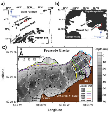
Fig. 1.Maps showing location of a. King George (25 de Mayo) Island, South Shetland Islands, and b. Potter Cove (PC). c. Location of hydrographic stations (black dots) in the inner PC. Stations were separated in two basins: in front to Carlini Station (Carlini Area: CA) and closer to the Fourcade Glacier (New Area: NA), represented by the dashed polygons. The white contour polygon represents the locations of profiles selected for calculating averages within NA. The glacier area retreated between 1956 and 2018 (coastline) is shown with colour lines (modified from Rückamp et al. Reference Rückamp, Braun, Suckro and Blindow2011). The glacier front in the water (December 2018) is marked in light blue. The shaded background displays the bottom topography (scale at right) in each panel. CAMS: Campbell Automatic Meteorological Station.
Two predominant modes of large-scale climate variability affect the Southern Ocean, particularly the Antarctic Peninsula region: the Southern Annular Mode (SAM; e.g. Thompson & Wallace Reference Thompson and Wallace2000) and the El Niño–Southern Oscillation (ENSO; e.g. Yuan Reference Yuan2004). The SAM is the main mode of variability of the Southern Hemisphere High Latitudes. It is directly associated with mid-latitude wind patterns, since it represents the exchange of atmospheric mass between lower and higher latitudes. This can be quantified by an index calculating the difference of zonal mean sea level atmospheric pressure between 40°S and 65°S latitudes, which fluctuates between positive and negative phases (Thompson & Wallace Reference Thompson and Wallace2000). This index presents a positive trend since the 1960s associated with an increase of westerly winds and the consequent air warming over the WAP (e.g. Marshall et al. Reference Marshall, Orr, van Lipzig and King2006). The ENSO, instead, is the main oscillation of the climate system on Earth, characterized by large-scale atmospheric pressure and sea surface temperature fluctuations in the equatorial Pacific affecting high latitudes of the Southern Hemisphere (Yuan Reference Yuan2004). During the negative phase of the ENSO (La Niña), a cyclonic circulation anomaly is located on the WAP, increasing the strength and frequency of north-westerly winds (Yuan Reference Yuan2004). This can lead to warmer air and water temperatures along the WAP, while the opposite pattern may occur during El Niño events (e.g. Stammerjohn et al. Reference Stammerjohn, Martinson, Smith and Yuan2008, Ruiz Barlett et al. Reference Ruiz Barlett, Tosonotto, Piola, Sierra and Mata2018). During the latter, warmer temperatures and less extent and duration of sea ice cover (SIC) are presented in the South Pacific while the inverse response is observed in the South-west Atlantic (Yuan Reference Yuan2004, Stammerjohn et al. Reference Stammerjohn, Martinson, Smith and Yuan2008). Fogt et al. (Reference Fogt, Bromwich and Hines2011) found that when SAM and ENSO are out phase (in phase), the ENSO teleconnection to the South Atlantic is stronger (weakened or absent). Conversely, the opposite response pattern is presented in the South Pacific region.
The Potter Cove system
Potter Cove (PC) is a semi-enclosed body of water located on King George (25 de Mayo) Island, South Shetland Archipelago (Fig. 1b). The area of the cove is approximately 7 km2 and its main axis has a SW–NE direction. The western edge is open to Maxwell Bay (Bahía Guardia Nacional). The northern and eastern coasts of PC are bounded by the Fourcade Glacier (FG; Fig. S1) while the southern coast is a beach of coarse sand and gravel (Wölfl et al. Reference Wölfl, Lim, Hass, Lindhorst, Tosonotto and Lettmann2014). Predominant winds are from the north-west and east (Klöser et al. Reference Klöser, Ferreyra, Schloss, Mercuri, Laturnus and Curtosi1994, Roese & Drabble Reference Roese and Drable1998, Schloss et al. Reference Schloss, Abele, Moreau, Demers, Bers, González and Ferreyra2012). In general, a cyclonic circulation allows the renewal of the PC waters that come from the northern side and leave through the southern sector. Furthermore, a vertical circulation cell exists with wind intensities higher than 5 m s-1, producing upwelling (downwelling) in the eastern edge of the cove during eastern (western) wind events (Roese & Drabble Reference Roese and Drable1998). Roese & Drabble (Reference Roese and Drable1998) postulated that tides are mixed with semidiurnal predominance and low-intensity tide currents.
The South Shetland Islands have a relatively moderate and humid climate compared to the PA region due to predominant westerly winds, its lower latitude and sea moderating effects (Schloss et al. Reference Schloss, Abele, Moreau, Demers, Bers, González and Ferreyra2012). Consequently, break and surface thinning of the coastal ice shelves have led to the retreat of coastal marine and tidewater glaciers (e.g. Rignot et al. Reference Rignot, Jacobs, Mouginot and Scheuchl2013). The low salinity surface layer in PC is formed during the meltwater season (summer) by the input of cascading glacial melt and melting of floating ice blocks and brash ice (that could also enter from the Maxwell Bay). Also, the southern coast presents a stream system during this season conditions (Fig. S1), with one creek due to precipitation (Matías Creek) and three due to glacial meltwater, which discharge surface and subterranean fine sediments (mainly silt) into the cove (Wölfl et al. Reference Wölfl, Lim, Hass, Lindhorst, Tosonotto and Lettmann2014, Monien et al. Reference Monien, Monien, Brünes, Widmer, Kappenberg and Busso2017). Of the latter, one has been called Potter Creek and the other two we have named unofficially “Oscar” and “Carlini” creeks. Monien et al. (Reference Monien, Monien, Brünes, Widmer, Kappenberg and Busso2017) estimated a meltwater discharge transport of 2–4 10-4 tons yr-1 of suspended particulate matter into the surface layer of the cove. Thus, during summer the PC circulation pattern is dominated by surface plumes of turbid, relatively warm meltwater that flow out of the fjord (e.g. Klöser et al. Reference Klöser, Ferreyra, Schloss, Mercuri, Laturnus and Curtosi1993, Reference Klöser, Ferreyra, Schloss, Mercuri, Laturnus and Curtosi1994) and depends on the stratification level controlled by freshwater input (Syvitski Reference Syvitski1989).
The annual mean Tair in the Jubany meteorological station, at Carlini (former Jubany) station, increased 0.66 °C between 1991 and 2009 (Schloss et al. Reference Schloss, Abele, Moreau, Demers, Bers, González and Ferreyra2012). These authors reported increasing sea surface temperature and total suspended particulate material in PC waters during this period, influencing a remarkable 20 km2 retreat of the FG (Fig. 1c) and significant loss of its glacier cover since the 1950s (Rückamp et al. Reference Rückamp, Braun, Suckro and Blindow2011). The FG has been a retreating tidal glacier (Rückamp et al. Reference Rückamp, Braun, Suckro and Blindow2011) that recently switched to a land terminating glacier, and its melting is strongly associated with local air temperature (Falk et al. Reference Falk, López and Silva-Busso2018, Meredith et al. Reference Meredith, Falk, Bers, Mackensen, Schloss and Ruiz Barlett2018). Subglacial meltwater inputs from the FG, mainly from the north-east coastline (Klöser et al. Reference Klöser, Ferreyra, Schloss, Mercuri, Laturnus and Curtosi1993, Reference Klöser, Ferreyra, Schloss, Mercuri, Laturnus and Curtosi1994), have decreased in recent years. Therefore, the meltwater and freshening dynamics are now mainly driven by surface runoff (Meredith et al. Reference Meredith, Falk, Bers, Mackensen, Schloss and Ruiz Barlett2018). The periodic ice supply is affecting benthic communities in shallow waters near the glacier, while glacier retreat generates new ice-free areas available for colonization (e.g. Sahade et al. Reference Sahade2015, Deregibus et al. Reference Deregibus, Quartino, Campana, Momo, Wiencke and Zacher2016). Several studies have analysed physico-chemical and biological processes within PC waters (e.g. Klöser et al. Reference Klöser, Ferreyra, Schloss, Mercuri, Laturnus and Curtosi1993, Reference Klöser, Ferreyra, Schloss, Mercuri, Laturnus and Curtosi1994, Deregibus et al. Reference Deregibus, Quartino, Campana, Momo, Wiencke and Zacher2016) and their relation with the climate variability, including ENSO and SAM (Bers et al. Reference Bers, Momo, Schloss and Abele2012, Schloss et al. Reference Schloss, Abele, Moreau, Demers, Bers, González and Ferreyra2012, Reference Schloss, Wasilowska, Dumont, Almandoz, Hernando and Michaud-Tremblay2014, Kim et al. Reference Kim, Ducklow, Abele, Ruiz Barlett, Buma and Meredith2018).
The aim of this article is to analyse the interannual variability of waters within the inner area of the PC during summers (January to February) from 2010 to 2017 and its connection with climate change. Studying the oceanographic processes that affect the cove waters has a vital importance to characterize and evaluate changes in the marine ecosystem. In order to study how physical characteristics of the Potter system can be affected by the contribution of melting water and glacier detachments, several oceanographic parameters (water temperature, salinity and turbidity) sampled in two regions of PC, near and away from the glacier front, plus atmospheric variables (Tair, precipitation and wind conditions), as well as monthly SIC data, were analysed. Then, the temporal variability in 3-layers of the area closer to the glacier was studied. Finally, we carried out a combined analysis of ENSO and SAM together with the hydrographic and atmospheric changes in the PC observed from 2009 till 2017.
Materials and methods
Meteorological and sea ice cover data
A Campbell Automatic Meteorological Station was installed each summer (January to February) from 2010 to 2017 near Elephant Point (62°14′16.1″S, 58°40′44.4″W), over the south-west extreme of the PC (Fig. 1c), a site near the mouth of the cove which is less affected by orography. Sensors of surface Tair and wind were placed at 8 m above sea level and their measurement rate was set at a frequency of 10 minutes. Time series of mean daily Tair and accumulated monthly wind roses during the eight summers of this period are shown in Fig. S2 and Fig. S3, respectively. Missing data were interpolated with daily means of the Jubany meteorological station (3-hourly frequency data) from the Servicio Meteorológico Nacional (SMN), the National Weather Service of Argentina. Also, daily accumulated precipitation was obtained from the SMN. Precipitation values on daily positive (negative) Tair are considered as rainfall (snow). Then, monthly means for each parameter and monthly predominant wind direction were obtained.
The area-averaged SIC fraction data were obtained from the MERRA-2 model M2TMNXFLX v5.12.4, available at https://giovanni.gsfc.nasa.gov/giovanni/ (GMAO 2015), which provides monthly time series with a 0.5° x 0.625° resolution. In this study we used the monthly mean of SIC between January 2009 and December 2016 at 58°45'W–58°36'W and 62°12'S–62°15'S.
Bathymetry data
The bathymetry transects were performed in PC with an integrated Garmin Echo sounder-GPS system onboard pneumatic boats during the summers 2010–12. Data were corrected by tide prediction and they were referred to mean sea level. Bottom marine topography (Fig. 1c) was obtained using the Kriging interpolation method. The coastline of the cove and south-west coast of the island near Carlini Station was measured with a Garmin GPS. A shallow sill (~30 m) separates the inner (55 m maximum depth) and outer (~200 m depth) areas (Klöser et al. Reference Klöser, Ferreyra, Schloss, Mercuri, Laturnus and Curtosi1994). In turn, the inner PC can be divided into two basins by a sill of about 25 m depth, which is located approximately in the western limit that had the glacier in 1956 (Rückamp et al. Reference Rückamp, Braun, Suckro and Blindow2011). The retreat of the FG resulted in a sea ice-free zone of 0.97 km2 from 1997 to 2010. Between February 2010 and December 2018, the FG has retreated 0.042 km2 in the east end and only 530 m of its cover is in the water in late 2018 (Fig. 1c).
Hydrographic data
The measurements of the physico-chemical parameters of the sea water column were conducted using a SBE 19plus V2 CTD (Conductivity, Temperature and Depth), with an auxiliary ECO NTU turbidity sensor. Sampling was carried out from pneumatic boats (wind conditions < 20 knots) during summer (January and February) over an 8-year period (2010–17). An oceanographic winch was used to reach the bottom waters in the inner cove (~55 m deep), except in 2010, 2012 and 2016, when the measurements were made in the first 30 m. We excluded observations with less than 1 m depth in order to homogenize the initial value and filter surface effect in CTD sensors such as wave rugosity and Tair. CTD data were processed using SBE Data Processing software. Then, potential temperature (θ), salinity (S) and potential density anomaly (σ) were calculated using the International Thermodynamic Equation of Seawater-2010 (TEOS-10; IOC et al. 2010), with precisions of 0.001°C in temperature and 0.0003 in salinity.
We considered two areas in the inner PC: one in front of the scientific station, Carlini Area (CA), and the other closer to the FG, New Area (NA), which is an ice free area due to glacier retreat since the 1950s. Schloss et al. (Reference Schloss, Abele, Moreau, Demers, Bers, González and Ferreyra2012) compared two stations far and near the FG in PC over 19 years. As a consequence of the glacier retreat, CA, which we compare with NA, coincides with the area previously near the FG used by these authors. Summer mean profiles and standard deviations of hydrographic properties were obtained to compare the vertical thermohaline structure in both areas. To study the temporal variability, we selected stations located in the central area of NA (Fig. 1c), to minimize spatial variability. The water column was separated in three depth strata: 1–5 m (surface water), 5–10 m (approximately the pycnocline location) and > 10 m (deep water). For each profile, we calculated mean values of the oceanographic properties for the three selected layers. Then, monthly means and standard deviations were estimated. In order to quantify the vertical stratification of the water column, Simpson's parameter (ϕ; as in Simpson et al. Reference Simpson, Allen and Morris1978) from each profile was calculated, and to analyse the stability conditions, Brunt-Väisälä or buoyancy frequency (N2; Millard et al. Reference Millard, Owens and Fofonoff1990) was determined. Both equations are presented in Supplementary Material as Eq. S1 and Eq. S2, respectively. Finally, mean and maximum monthly values were estimated for the analysed 8-summer period.
ANOVA and correlations
Non-parametric Kruskal-Wallis one-way ANOVA test was used to compare the daily means of the oceanographic parameters between the two areas (CA and NA) and between the surface and the deepest layer (> 10 m) in each area. Also, an ANOVA test followed by a Bonferroni post-test was used to compare monthly and interannual means in the central region of NA. The test was applied to monthly means of Tair and SIC for a whole year, to summer Tair and precipitation (Tair ≥ 0 °C) and oceanographic variables. Cross-correlations were made to determine Kendall's correlation coefficients. These correlations were carried out between monthly means of Tair, SIC and climate variability modes (ENSO and SAM) as well as with the hydrographic averages of the shallow and the deepest NA layers. The significance level was P < 0.05 for correlations with oceanographic parameters and P < 0.01 in remaining cases.
Results
Meteorological summer conditions in Carlini Station (2010–17)
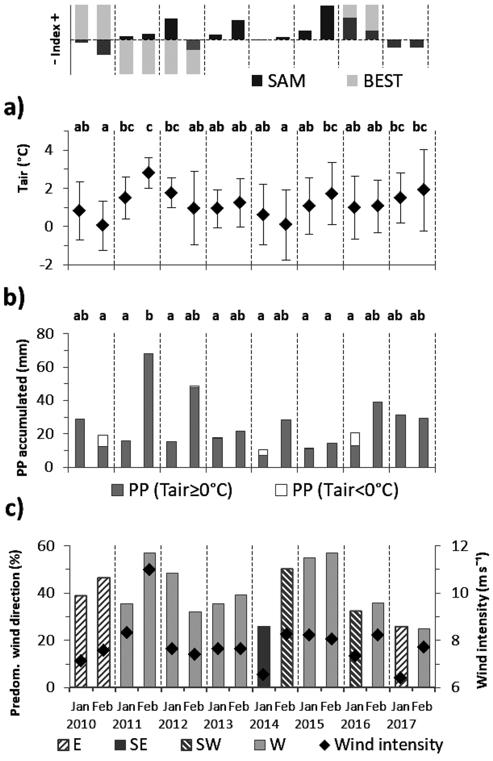
January and February monthly mean of Tair show high monthly and interannual variability during the period 2010–17 (Fig. 2 and Table S1). Summer 2011 was warm while 2010 and 2014 were cold summers (Bonferroni ANOVA, P < 0.05). Monthly Tair means for 2010–17 summers are 1.14 ± 0.39°C (January) and 1.23 ± 0.93°C (February), statistically not different. The maximum daily Tair (9.66°C) was recorded on 1 January 2016 while the minimum (-6.24°C) was observed on 9 February 2014. February 2011 was the warmest and rainiest month with the highest mean wind intensity and westerlies frequency. Alternatively, during predominant easterlies in February 2010 and southerlies in January 2014, respectively, colder summers were observed with a fraction of precipitation in negative daily temperature (snow) conditions.
Fig. 2.Monthly values at Carlini Station of a. mean near-surface air temperature (Tair; represented by diamonds) with one standard deviation (vertical bars), b. accumulated precipitation (PP) of rainfall (Tair ≥ 0 °C) and snow (Tair < 0 °C) and c. percentage of occurrence of monthly predominant wind direction from east (E), south-east (SE), south-west (SW) and west (W). Diamonds represent wind intensity monthly means associated with predominant directions. Different letters represent significant differences (ANOVA test followed by a Bonferroni post-test, P < 0.05) between months during the eight-summer period for a. Tair and b. rainfall. Shared letters indicate non-significant differences. SAM and BEST (ENSO) monthly index during January and February are shown above panel a.
Hydrographic properties of Potter Cove
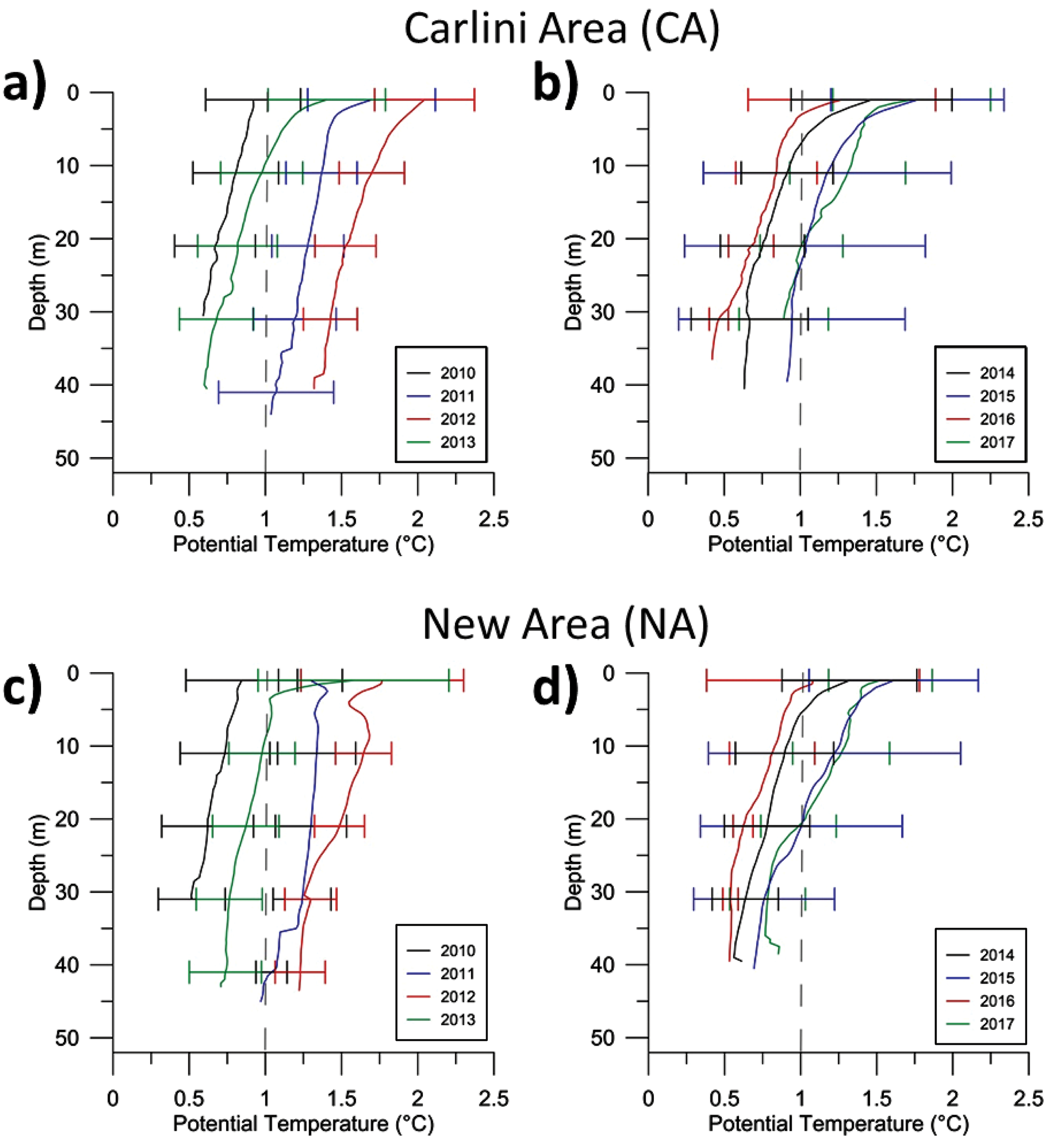
The interannual mean θ profiles do not present significant differences between CA and NA (Fig. 3 and Table I), although the Kruskal-Wallis ANOVA showed significant differences between shallow and deeper waters within each area. Air temperature-induced θ conditions originate at the water surface and propagate downward into the water column by wind-induced mixing. Thus, warmer summers are visible throughout the entire water column (< 50 m deep). The water column was warmer in summer 2012 while the coldest waters were observed in 2010. The maximum θ range in the PC waters resulted between 0.047 and 2.864°C, with its maximum value recorded in surface waters on 13 February 2015. In fact, 2015 presented the highest θ variability, while the most homogeneous profiles were obtained in 2010. When comparing January and February each summer (Fig. S4), some interesting aspects deserve to be pointed out. In general, θ decreases with depth although some profiles presented warming from the surface to a subsurface maximum and then the waters become colder as the depth increases (February 2011, 2012 and 2016). During summers of 2011, 2013 and 2015, θ profiles for February were warmer than January. The lowest mean θ was obtained in January 2015, although they were calculated from a daily single profile. At the time of the measurement (8 January) and in the previous hours, the wind was predominant from the glacier direction (easterlies), which resulted in Tair values lower than -1.5°C. In January 2016, the water column was more stratified and warmer than in February, although few sampling days were carried out during this summer due to adverse weather conditions.
Fig. 3.Mean potential temperature (θ) profiles a., b. in the CA, and c., d. NA for the period 2010–13 and 2014–17, respectively. Horizontal bars represent one standard deviation around the mean of certain chosen depth. Vertical dashed line represents 1°C.
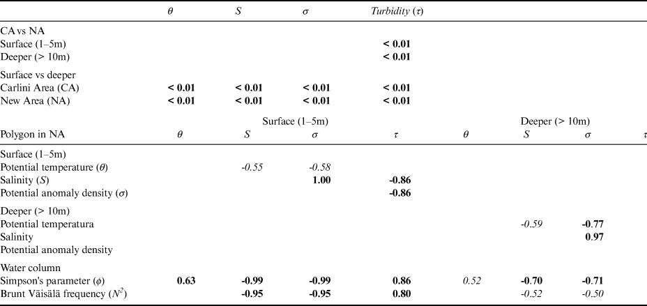
Table I.Upper panel: Results of Kruskal-Wallis one-way ANOVA comparing areas (CA and NA) and water layers in PC. Lower panel: Significant correlations (at 95% in italic and 99% in bold) between hydrographic parameters into the black polygon in NA.
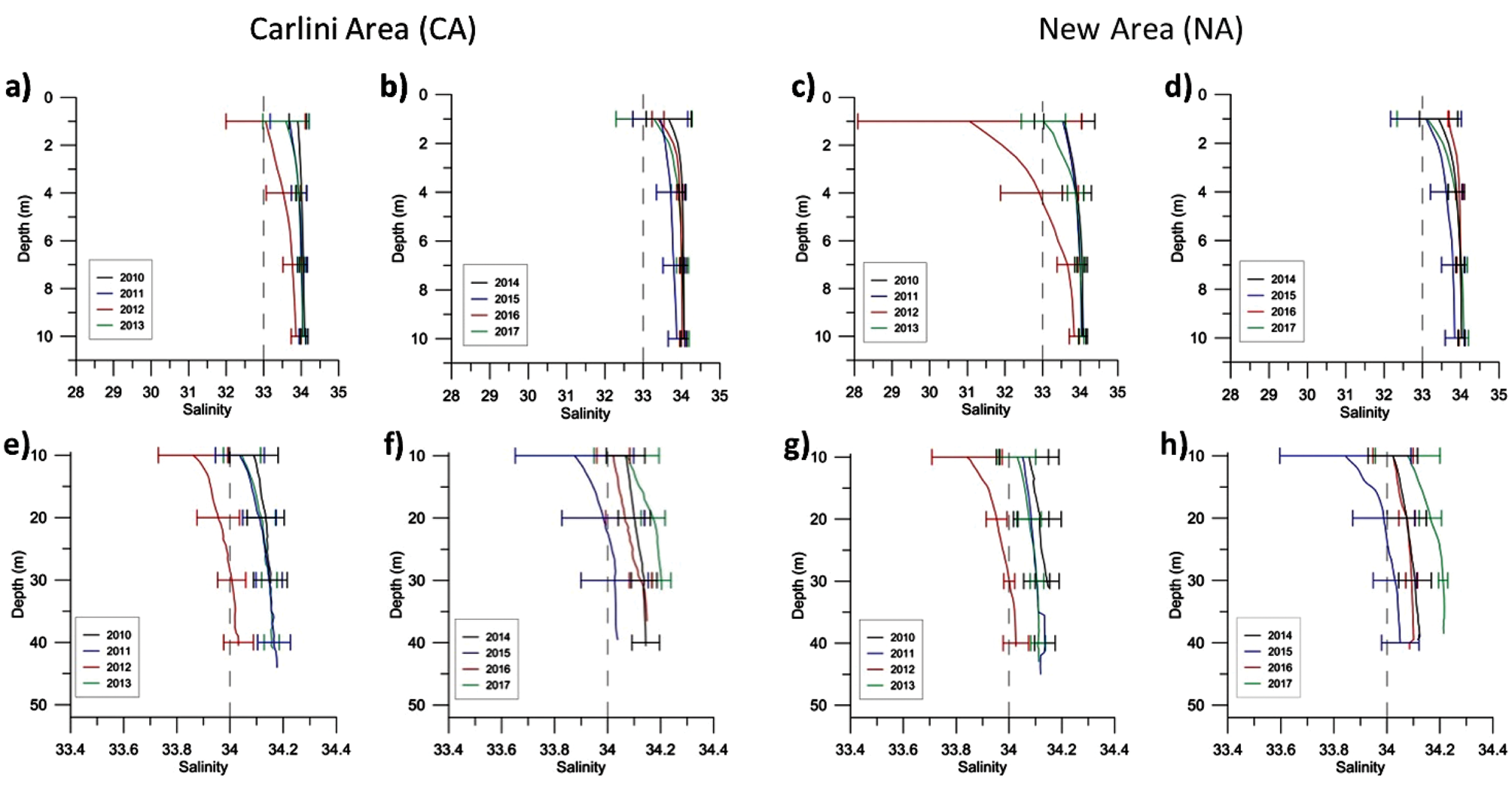
The structures of the mean S profiles between CA and NA obtained in the deepest layer were more similar to each other than those of the shallower layer (Fig. 4). However, only the difference between surface and deeper layers within each area are statistically significant (Table I). The stratification in the first meters of the water column shows the freshwater input from FG and glacio-fluvial creeks, more visible in NA during summers of 2012 and 2013. The mean θ profiles in 2012 and 2015 (> 4 m) resulted fresher compared to the rest of summers in both areas. January was less saline than February in 2010, 2012 and 2017 (Fig. S5). The θ-S diagrams in Fig. S6 shows high inter-annual and summer variability of the thermohaline properties in the PC water column. Low S was observed in surface waters both in relatively warm and cold conditions, since changes in density layers in fjords like PC are mainly affected by variations in S due to glacier freshwater inputs during summer.
Fig. 4.Mean salinity (S) profiles a., b., e., f. in the CA, and c., d., g., h. NA for the period 2010–13 and 2014–17, respectively. Horizontal bars represent one standard deviation around the mean of certain chosen depth. Upper panel represents 1–10 m depth layer and lower panel represents deeper than 10 m. Note the different scales between both panels. Vertical dashed line represents S of 33 (upper panel) and 34 (lower panel).
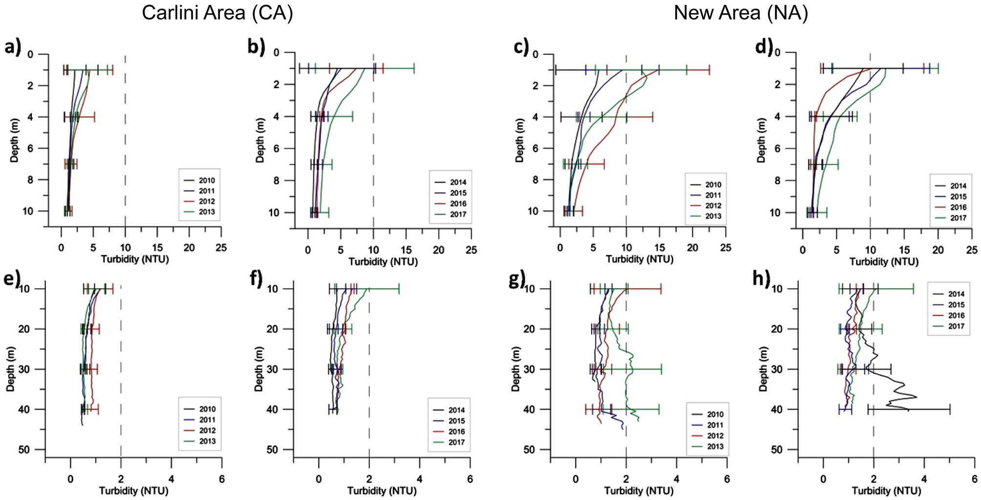
Mean turbidity (τ) profiles show increasing values in the surface layer of the CA (Fig. 5a & b). Instead, high interannual variability is visibly in the NA (Fig. 5c & d). Here, surface τ values nearly to 30 NTU were reached several times (Fig. S7). On the other hand, deeper waters near the mouth of the inner cove showed very low turbid values, although were relatively higher during 2012 and 2017 (Fig. 5e & f). In general, τ values decrease with depth. However, during some summers (mainly 2013 and 2014) high τ values in deeper waters (>10 m) were recorded by several CTD profiles located in the PC eastern edge (Fig. 5 g & h). These turbid deep waters were present both in January and February (Fig. S7). In particular, 2014 reached values greater than 10 NTU in waters deeper than 20 m. Turbidity shows significant differences (P < 0.05) between both areas and shallow and deeper waters (Table I). Finally, high τ values were recorded both during low and relatively high S conditions (Fig. S8), reaching a maximum of 29.25 NTU on 25 January 2010 in the surface layer near the glacier. During January 2012 extremely low surface S values were found in PC waters compared to other observations obtained during similar maximums τ conditions (~30 NTU). It may be associated with higher contribution of freshwater input from the glacier because of relatively warm air conditions on the cove and melting of floating ice blocks. Correlations between S and τ in the water column will be explored in the Discussion.
Fig. 5.Mean turbidity (τ) profiles a., b., e., f. in the CA, and c., d., g., h. NA for the period 2010–13 and 2014–17, respectively. Horizontal bars represent one standard deviation around the mean of certain chosen depth. Vertical dashed line represents τ of 10 (upper panel) and 2 NTU (lower panel).
Interannual variability of hydrographic properties in the New Area (NA)
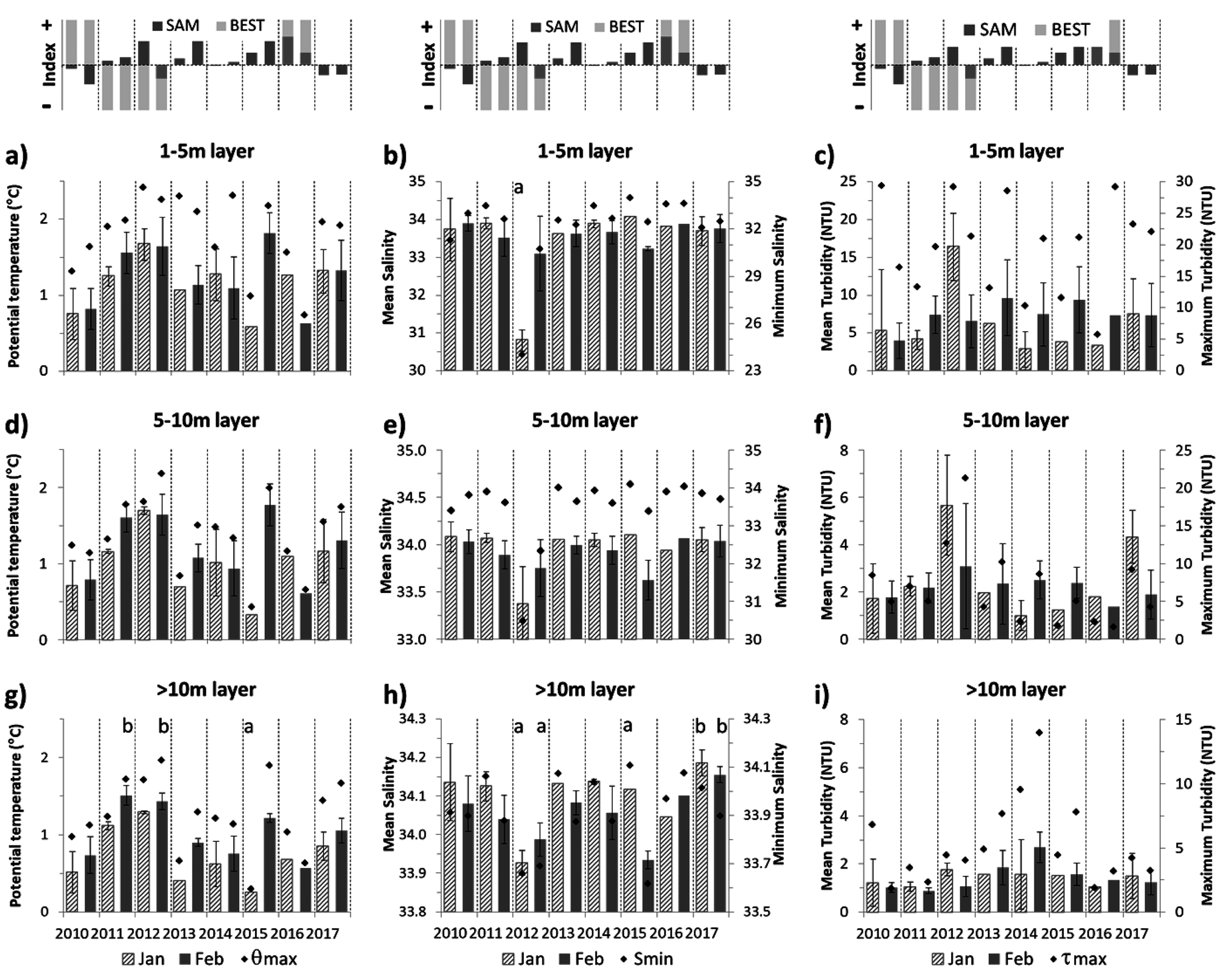
For each of the 3 layers in which the central region of the NA (see Fig. 1c) was vertically divided, we found significant differences between monthly mean hydrographic properties during the 8-summer period, from 2010–17. Summer θ in surface waters (1–5 m layer) resulted significantly colder in 2010 and warmer in 2011 and 2012 (Bonferroni ANOVA, P < 0.05). A similar analysis that showed the summer S of 2012 was significantly lower than the remaining summers. Also, February 2015 presented the warmest mean surface waters (1–5 m layer; Fig. 6a), while the monthly mean significantly less saline and highest τ mean were observed in January 2012 (Fig. 6b & c). Even though high values (~30 NTU) were observed several times, it indicates a τ threshold in this region (Fig. 6c). Mean summer hydrographic values in the surface layer and their standard deviations are shown in Table II.
Fig. 6.Monthly averages for sea surface values (1–5 m depth range) of a. θ, b. S and c. τ for the oceanographic stations selected in the polygon within NA (see Fig. 1c). The vertical bars represent a standard deviation around the media. Maximum of θ and τ, and minimum of S, recorded in each month are shown with black diamonds in the corresponding panel. Idem for a range of 5–10 m depth (central panel) and > 10 m (lower panel). Different letters represent significant differences (ANOVA test followed by a Bonferroni post-test, P < 0.05) between months during the eight-summer period in surface and deeper layers. Consider the change in the vertical axis scale in S and τ, between panels and each one. SAM and BEST monthly index during January and February are shown above the upper panel.
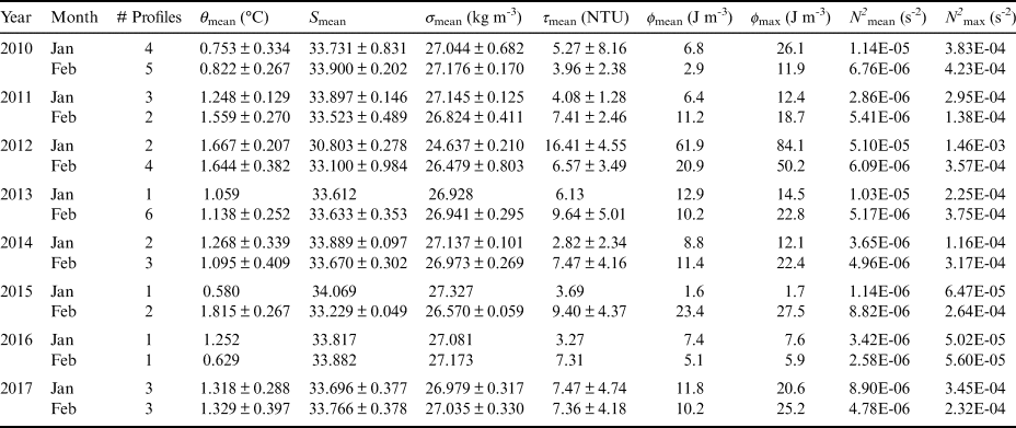
Table II.Monthly means and standard deviation of physical variables (in 1–5 m deep range), Simpson's parameter (ϕ) and Brunt-Väisälä frequency (N2) (in the water column) into the NA polygon for January and February. The monthly maximum value of ϕ (ϕ max) and N2 (N2 max) also is mentioned. Profile numbers available for each month is indicated.
The same pattern showed in the surface for S and θ can be observed in the 5–10 m depth layer (Fig. 6d & e). In this layer, a monthly mean of τ higher than 5 NTU and the highest value (~20 NTU) were found during summer 2012 (Fig. 6f). In the deepest layer (> 10 m), θ variations are similar to those in the 5–10 m layer (Fig. 6g), although different patterns were detected in S and τ (Fig. 6h & i). In these waters, February 2011 and 2012 were significantly warmer while January 2015 was colder (Bonferroni ANOVA, P < 0.05). On the other hand, significantly fresher waters were found in summer 2012 and February 2015, while summer 2017 was the most saline. Low S values in the deepest waters may be associated with more westerly winds (Fig. 2b), which favours downwelling near the glacier, moving the less saline and lighter superficial waters into the water column. At this layer, in most of the study period, February is significantly warmer and fresher than January (Bonferroni ANOVA, P < 0.05). Relatively high mean τ in the summers of 2013 and 2014 were detected, reaching a maximum value of 13.96 NTU (~40 m depth) in February 2014 (Fig. 6i).
The highest monthly mean and maximum values of ϕ and N2 in the PC water column near the glacier were obtained in January 2012 (Table II). The stratification degree found in 2012 was significantly higher than that obtained during other summers of the study period (Bonferroni ANOVA, P < 0.05), which is associated with the lowest S conditions in PC surface waters. In contrast, the lowest mean values of ϕ and N2 were obtained in January 2015, which indicate a relatively homogeneous water column (except a thin surface warmer in the first meters), typical of the pre-melting season (spring).
The correlations obtained between thermohaline parameters and τ (in the surface and deeper layers), ϕ and N2 are presented in Table I. High density dependence with changes in S was observed, with less influence from θ, especially in the surface layer. A statistically significant inverse correlation between S and τ was found, which is linked to the contribution of sedimentary material from the runoffs and glacial detachment. Significant positive (negative) correlations were obtained between ϕ versus surface θ and τ (S and density). Also, N2 resulted in a positive (negative) link with τ (S and density) in lower coefficients. Moreover, in deeper waters the thermohaline influence is presented in both stratification parameters (except between θ and N2).
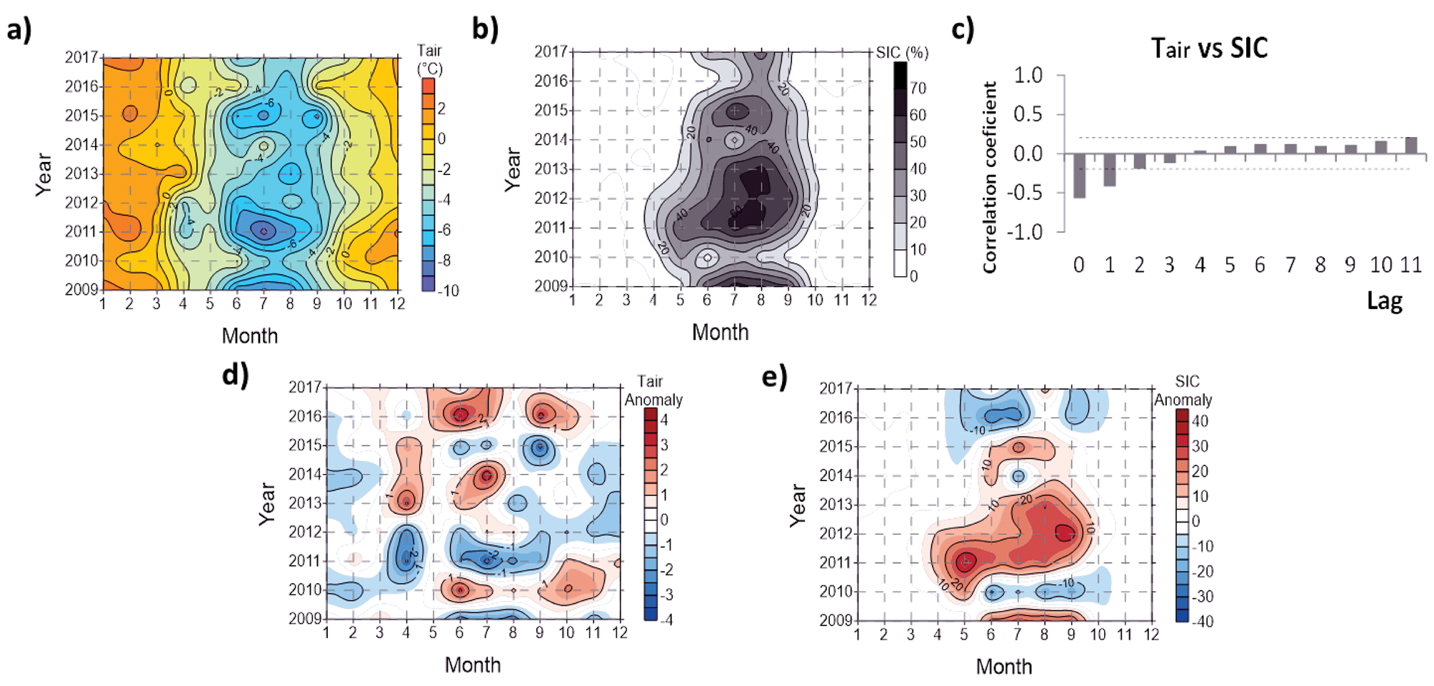
Cross-correlations between SIC and Tair (Fig. 7a & b) were significantly negative with 0 and 1-month lags (Fig. 7c). During winter and spring of 2010, 2014 and 2016 there were positive Tair anomalies, leading to less SIC (Fig. 7d & e) and early ice-breaking. Conversely, negative Tair anomalies during winters of 2009, 2011, 2012 (early and short-time winter) and 2015 led to higher and more persistent values of SIC over time, mainly during the spring of 2009 and 2012. A statistical ANOVA analysis (P < 0.05) reveals significantly extreme winters with lower SIC (2016, and to a lesser extent 2010) and higher SIC (2011 and 2012, and to a lesser extent 2009).
Fig. 7.Hovmöller diagram of a. Tair and b. sea ice cover (SIC) percentage during the period 2009–17. c. Cross-correlations between monthly Tair and SIC for the historical dataset of PC (1987–2017). Each lag corresponds to one month. Horizontal dotted black lines represent confidence bounds at 99%. d. Tair and e. SIC anomalies calculated from the historical dataset.
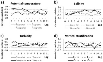
Finally, the rank cross-correlations of oceanographic parameters in NA with Tair and SIC are shown in Fig. 8, with lags between 0 and 11 months. The monthly mean Tair was significantly positive correlated with θ in surface and deeper waters (between lags 0 and 3; see Fig. 8a). Also, significant negative correlations were observed between SIC and θ (4-month lag) in the deep layer. On the other hand, a significant negative relationship between Tair and surface S was obtained with a one-month lag (Fig. 8b). Additionally, a significant positive correlation was seen in lag 1 between Tair and surface τ (Fig. 8c) and vertical stratification parameters of the water column (Fig. 8d). There are some significant remaining values which would not be physically possible. For instance, the link between SIC and θ (at depth layer > 10 m) in lag 0, there are no measurements in the water column when SIC was present.
Fig. 8.Cross-correlation between monthly Tair and SIC with hydrographic parameters inside the NA polygon. Each lag corresponds to one month. Horizontal dotted black lines represent confidence bounds at 95%.
Discussion
Hydrographic comparisons between the two areas of inner Potter Cove
Several authors reported lower values of surface temperature in waters near FG than in those bordering Maxwell Bay during summers (e.g. Klöser et al. Reference Klöser, Ferreyra, Schloss, Mercuri, Laturnus and Curtosi1994, Garcia et al. Reference Garcia, Hoffmeyer, López Abbate, Barría de Cao, Pettigrosso and Almandoz2016). Additionally, summer S values in a thin surface layer increase outwards, where the influences of the FG is less important (Fig. 4, upper panel; Klöser et al. Reference Klöser, Ferreyra, Schloss, Mercuri, Laturnus and Curtosi1994, Garcia et al. Reference Garcia, Hoffmeyer, López Abbate, Barría de Cao, Pettigrosso and Almandoz2016). However, no significant thermohaline differences are observed between the two regions of inner PC: CA and the region closer to the glacier, NA (Table I). On the other hand, the S range during the 8-summer study period in PC was similar to the climatological summer range obtained during the previous years by Schloss et al. (Reference Schloss, Abele, Moreau, Demers, Bers, González and Ferreyra2012), and also in the nearby Marian Cove by Lee et al. (Reference Lee2015) and Gerlache Strait bays by Rodrigo et al. (Reference Rodrigo, Giglio and Varas2016).
Significant differences were found in the thermohaline properties between surface and deeper layers in each area in PC, similar to those obtained between two stations, in front of Carlini Station and outer cove, by Schloss et al. (Reference Schloss, Abele, Moreau, Demers, Bers, González and Ferreyra2012). Falk et al. (Reference Falk, López and Silva-Busso2018) found that 84% of the changes in FG discharge can be explained by Tair changes. In shallow waters near the glacier influence on fjords, warmer summers lead to more stratification by freshwater input for example, due to cascading glacial melt, subglacial and creeks meltwater, floating ice blocks during minimal wind intensity conditions (e.g. Syvitski Reference Syvitski1989, Klöser et al. Reference Klöser, Ferreyra, Schloss, Mercuri, Laturnus and Curtosi1993, Reference Klöser, Ferreyra, Schloss, Mercuri, Laturnus and Curtosi1994). As density depends mainly on S changes both in high latitudes open sea or a fjord as PC, when the surface layer is fresher and thicker in the water column, higher vertical stratification is observed during the melting season (e.g. Syvitski Reference Syvitski1989, Schloss et al. Reference Schloss, Abele, Moreau, Demers, Bers, González and Ferreyra2012, Rodrigo et al. Reference Rodrigo, Giglio and Varas2016, Höfer et al. Reference Höfer2019). Thus, the highest ϕ values obtained in this study are consistent with Falk et al. (Reference Falk, López and Silva-Busso2018) model results. The water column presents a strong stratification under low mixing conditions due to lower wind intensity and a higher inflow of fresh water from the FG (Schloss et al. Reference Schloss, Abele, Moreau, Demers, Bers, González and Ferreyra2012). These authors reported a significant water temperature influence on the water column stratification of the inner cove, and therefore a local forcing. In this study, connections between Tair, thermohaline and stratification parameters of the NA waters were found (Fig. 8 and Table I). In consequence, changes in the atmosphere on PC are reflected in θ and S and then, in the vertical structure of the water column, which shows the local meteorological and glacier melt influence into cove waters (Schloss et al. Reference Schloss, Abele, Moreau, Demers, Bers, González and Ferreyra2012). This is probable because the melting of FG is mainly related to Tair and not to basal melting since the glacier is almost entirely on land now (Falk et al. Reference Falk, López and Silva-Busso2018, Meredith et al. Reference Meredith, Falk, Bers, Mackensen, Schloss and Ruiz Barlett2018).
Significant differences of τ were observed between the regions closer to the FG (NA) and the less turbid offshore (CA) during the summers of 2010–17, both in surface and deeper waters. Similarly, for summers of 2010–13, Deregibus et al. (Reference Deregibus, Quartino, Campana, Momo, Wiencke and Zacher2016) reported significantly different mean τ values of 7.52 ± 2.21 NTU and 3.49 ± 0.86 NTU in the 0–10 m depth layer, near to Isla D (see Fig. 1c) and the northern coast of PC, respectively. High τ values in the thin surface layer (negative linked with S) also have been observed in other glacial bays of the South Shetland Islands and are higher than those found in other Antarctic regions as the Gerlache Strait bays (see locations in Fig. 1a; e.g. Rodrigo et al. Reference Rodrigo, Giglio and Varas2016, Lima et al. Reference Lima2019). Turbid waters in the first meters restrict the light penetration for photosynthesis into the water column, which limits benthic and pelagic primary production in the inner cove waters (e.g. Schloss et al. Reference Schloss, Abele, Moreau, Demers, Bers, González and Ferreyra2012, Sahade et al. Reference Sahade2015, Deregibus et al. Reference Deregibus, Quartino, Campana, Momo, Wiencke and Zacher2016). The latter authors obtained a positive correlation between the penetration of light and the maximum depth limit in the presence of macroalgae, which, in turn, decreases with the proximity to the glacier.
The formation of the high τ plume and its vertical structure in fjords seem to be determined by the buoyant equilibrium (Syvitski Reference Syvitski1989, Rodrigo et al. Reference Rodrigo, Giglio and Varas2016). Schloss et al. (Reference Schloss, Abele, Moreau, Demers, Bers, González and Ferreyra2012) did not find a significant correlation between N2 and total suspended particulate matter in front of the Carlini Station area. Conversely, a positive link was obtained between τ in the surface layer with ϕ and N2 parameters of the NA water column (Table I), which reflects how the cloudy plume of water is “trapped” within the thin layer of fresher water (e.g. Rodrigo et al. Reference Rodrigo, Giglio and Varas2016). Also, the sediments distribution within the fjord is largely controlled by the circulation in the first meters (Syvitski Reference Syvitski1989). Westerly winds increase the thickness of the subsurface layer of water coming out from the inner cove, which could favour the export of suspended sediments (Roese & Drable Reference Roese and Drable1998). In consequence, the relatively clear waters with little sedimentary content entering from Maxwell Bay in the summer renew the PC turbid waters due to sedimentary meltwater contribution. Monien et al. (Reference Monien, Monien, Brünes, Widmer, Kappenberg and Busso2017), using sediment traps, determined that a significant percentage of suspended particulate material (15% to 50%) is horizontally exported and leaves the inner cove.
High values of τ have been observed in the deepest layer of the NA water column (Fig. 6i), as well as in deep waters near glaciers in other Antarctic fjords (e.g. Rodrigo et al. Reference Rodrigo, Giglio and Varas2016). These have been associated with a sediment source that emerges from under the tidal glacier at the head of each bay and flows outwards. However, the subglacial freshwater discharge (including surface and basal runoff) from FG in the calving front would be colder and fresher than observed in PC. Only during January 2011 a slight increase in turbidity in the deepest waters (Fig. S7) related to the decrease in temperature and salinity was present (not shown). In consequence, other hypotheses to explain the mechanism of these turbid layers should be considered. For instance, the transport of particles from the seabed associated with currents driven by tides and/or wind. One such high turbidity deep water event near the glacier was present on 16 February 2013. A glacier discharge event in the previous 10 days was studied by Meredith et al. (Reference Meredith, Falk, Bers, Mackensen, Schloss and Ruiz Barlett2018). They postulate that glacial discharge of freshwater and suspended particulate material observed between February 6 and 11 could have been exported laterally and towards the seabed days later. The strong katabatic winds recorded between 11 and 13 February could have favored the vertical mixing and resuspended the recent soft sediment that penetrated the cove. As they are denser waters than surrounding sea water and N2 values are close to zero (not shown), these turbid waters would keep trapped by the ridge encloses the so-called “New Area” to the west, until the vertical mixture disperses these particles towards surface waters and/or out of PC.
Climate conditions on Potter Cove for the 2010–17 summer period
The mean summer (January–February) temperature during the 8-summer period turned out to be colder (P < 0.01) than 1991–2009, according to SMN data (see Fig. S9). Thus, the warming of 0.39°C decade-1 in summer (December–February) between 1991 and 2009 (Schloss et al. Reference Schloss, Abele, Moreau, Demers, Bers, González and Ferreyra2012) has been attenuated over the last years. This result coincided with previous studies that report a period of no warming since the early 2000s in the Antarctic Peninsula region (Turner et al. Reference Turner2016). Also, Schloss et al. (Reference Schloss, Abele, Moreau, Demers, Bers, González and Ferreyra2012) reported a mean Tair of 2.5 ± 0.49 °C in January (the warmest month at Carlini Station), ~1.4°C warmer than that obtained for the period 2010–17. In our study period, February was 0.11°C warmer (not significant at 95% level) than January, which could explain the warmer and fresher deepest layer (> 10 m) in February compared to the previous month in the NA.
The FG has continued to retreat in recent years despite being a colder period (Fig. 1c). It should contribute to an input of sediment and freshwater to the cove by the PC streams system (e.g. Falk et al. Reference Falk, López and Silva-Busso2018). As mentioned before, the glacier limit is now on land since recent years (Meredith et al. Reference Meredith, Falk, Bers, Mackensen, Schloss and Ruiz Barlett2018). This change seems to have occurred between 2003 and 2013, which could have been favored by warm events with a large supply of fresh water, such as those observed during the summers 2011–12. Currently, the front of the glacier on surface water in the east extreme is no longer than 550 m (December 2018). Therefore, not only the input below the glacier of freshwater and sediment significantly decreased, but also less amount of pure freshwater would be contributing to the cove due to the rupture and cascades of the FG coastal ice shelf. We think this is an interesting result because it differs from other fjords in the Antarctic Peninsula where tidal glaciers are mainly melting due to sea water temperature (e.g. Rodrigo et al. Reference Rodrigo, Giglio and Varas2016). Lee et al. (Reference Lee2015) affirm that the glacier retreat in Marian Cove (neighbour to PC; see location in Fig. 1b) would not affect the surface S obtained at the continuous sampling site during 1998–2008. This situation is probably maintained today, because the glacier front in this fjord is largely over the water and does not exhibit meltwater creeks. Therefore, glacier melting should be associated with temperature changes in waters that enter Marian Cove from Maxwell Bay. Thus, differences in the geographical configuration of two very close fjords lead to important differences in the dynamics of the environment that surrounds them.
Unfortunately, the Jubany meteorological station does not have a device that allows us to distinguish rainfall from snow precipitation. The highest amount of precipitation during the studied summer months was detected on days with Tair above 0 °C. This allows us to infer that it was rainfall precipitation. The local increase of precipitation observed in recent years (Uotila et al. Reference Uotila, Lynch, Cassano and Cullather2007) could be related to the intensification of westerly winds and warmer air conditions, related to the positive SAM trend since the 1960s (Marshall et al. Reference Marshall, Orr, van Lipzig and King2006). Therefore, it may cause more glacier surface and subglacial erosion and the formation of new ways of water discharge increasing the input of sediments. From a model run, Jerosch et al. (Reference Jerosch, Scharf, Deregibus, Campana, Zacher and Pehlke2019) predict a reduction in the distribution and production of the macroalgal community in the coming years due to the increase in sedimentation of the FG retreat.
Predominant easterlies and westerlies in Carlini Station during the 8-summer period are in agreement with the wind pattern previously reported by other authors (e.g. Roese & Drable Reference Roese and Drable1998, Schloss et al. Reference Schloss, Abele, Moreau, Demers, Bers, González and Ferreyra2012). The pattern of water circulation in PC strongly depends on the intensity and direction of the wind, with a vertical circulation in response to wind direct effect and an opposite flux in deeper waters (Roese & Drable Reference Roese and Drable1998). As a consequence, the east (west) wind component generates upwelling (downwelling) flux in the PC eastern limit (bounded by the FG). Changes in Tair on the cove are strongly related to the variability of wind direction. Warmer air conditions during westerlies (particularly February 2011) and colder during easterlies and southerlies (summer 2010 and 2014) were observed in the study period (Fig. 2). Westerlies are related with warm advection of maritime air masses from the ice-free Bellingshausen Sea whereas easterlies are associated with cold advection due to colder conditions on the Weddell Sea region (e.g. Schloss et al. Reference Schloss, Abele, Moreau, Demers, Bers, González and Ferreyra2012). Furthermore, the location of the FG to the east of PC may also favour even colder advection of easterlies, which may be more associated to snow precipitation in summer months since monthly mean temperatures are slightly warmer than 0 °C. On the other hand, only rainfall was observed during predominant westerlies at Carlini Station.
High temporal variability has been observed in τ into the entire NA water column (Fig. 6, right panel). In general, high τ values were associated with relatively low S values in surface waters, which indicate that meltwater streams are the main source of suspended sediments as has been reported by other authors (e.g. Klöser et al. Reference Klöser, Ferreyra, Schloss, Mercuri, Laturnus and Curtosi1994). Changes in the τ-S relation due to the turbid meltwater could be caused both by the contribution of fresh water directly from the glacier and the glacial-fluvial rivers with terrigenous sediments. January 2012 clearly shows this situation when extremely low S values were associated with very turbid waters (Fig. S8). Maximum ϕ and N2 values were obtained in this month linked with the fresher surface layer present within the inner PC (Table II). A previously warm December (not shown) and the consequently larger glacial freshwater input could lead to this anomalous fresher waters. In addition, the intense wind favoured the mixing of the water column and resulted in an increase in the thickness of the surface layers of S and τ compared to the rest of the period (Fig. 4c and Fig. 5c, respectively). Although the measurements are carried out under relative low wind speed conditions (< 20 knots), sometimes a homogeneous water column is recorded as a result of previous strong and persistent winds. Thus, it is more probable to obtain a more stratified vertical structure during a relatively long calm period.
During 2012 high values of SIC were still present in October on PC waters, which are associated with negative Tair persistent anomalies during winter and spring seasons (Fig. 7). The same pattern was observed during winter 2011, although a warm spring and persistent strong wind (not shown) led to melting and an earlier sea ice retreat than 2012. Conversely, early breaking occurred during the spring of 2010 and 2016 both warm winters with the lowest SIC over the study period. Particularly in 2016, the relationship between low SIC and early breaking during anomalously positive Tair is followed by “normal” air conditions during late spring and summer. Significant low S values in the deeper layer during summer 2012 (Fig. 6h) suggest both an anomalous early meltwater and downwelling from the fresh surface layer near the FG. On the other hand, significantly higher S monthly means in deeper waters were observed during summer 2017. Thus, the effects of winter SIC and time of sea ice breakout could be evidenced first in Tair and a few months later, in θ of the NA deeper layer (Table I). In warm years, when the SIC period is shorter, the effect of stronger winds deepens the mixed layer and therefore requires greater buoyancy to be stabilized, leading to a persistent reduced stratification during spring–summer (Kim et al. Reference Kim, Ducklow, Abele, Ruiz Barlett, Buma and Meredith2018). The favourable light conditions for the growth of algae are maintained after the break of the winter sea ice layer and until the turbid fusion waters enter the cove 2 to 3 months later (Wiencke & Amsler Reference Wiencke, Amsler, Wiencke and Bischof2012). Therefore, the time of sea ice breaking and amount of sediment that reaches the cove and the time in which it occurs are of extreme importance for algae (Deregibus et al. Reference Deregibus, Quartino, Campana, Momo, Wiencke and Zacher2016).
Connections between climate variability modes and interannual oceanographic and atmospheric PC changes
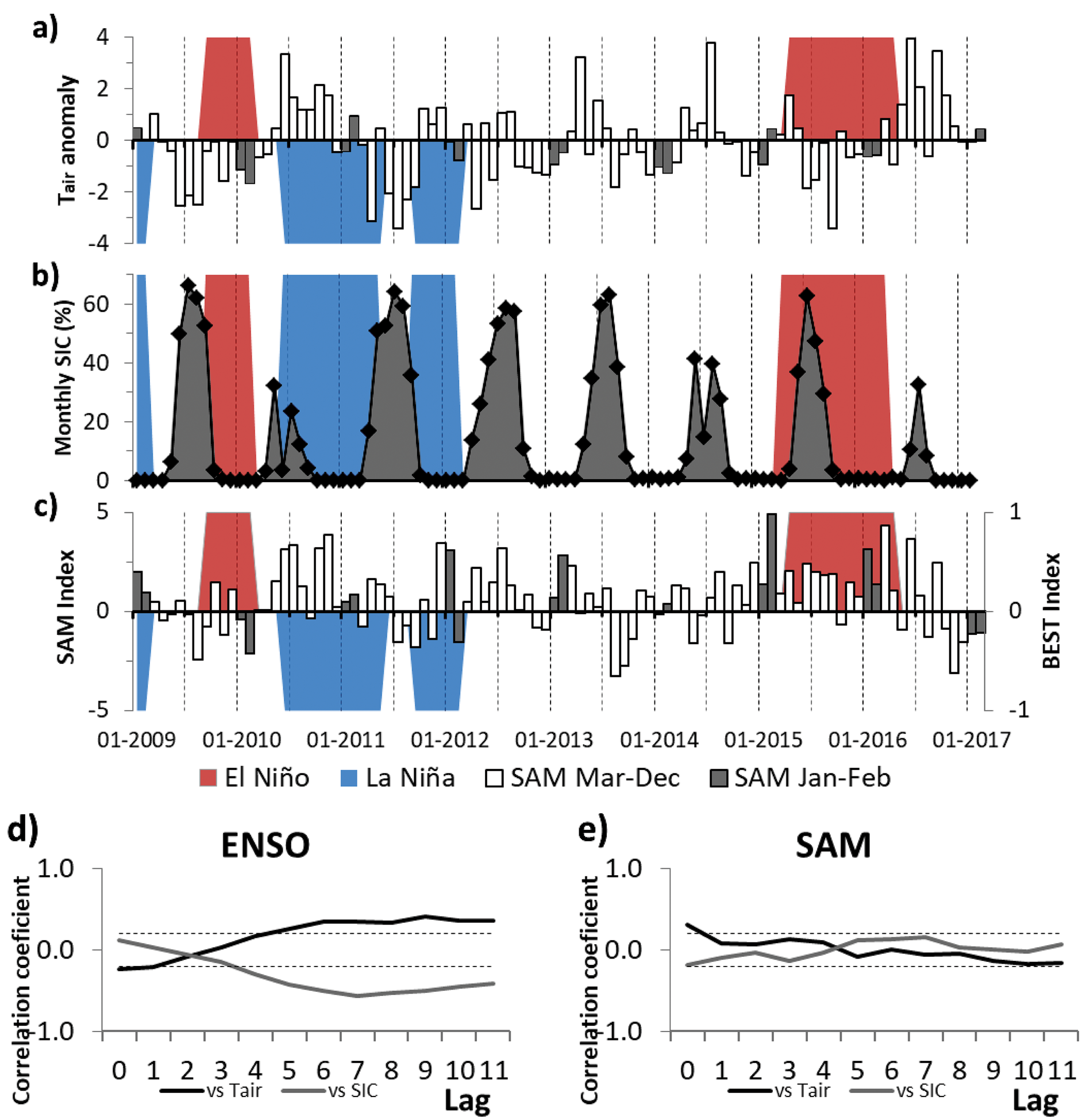
Since ENSO is the main mode of variability of the Earth System and SAM the main mode of the atmosphere of southern high latitudes, it is very well documented the relation these modes may haven with the Antarctic region (e.g. Yuan Reference Yuan2004, Stammerjohn et al. Reference Stammerjohn, Martinson, Smith and Yuan2008, Ruiz Barlett et al. Reference Ruiz Barlett, Tosonotto, Piola, Sierra and Mata2018). Therefore, to explore and further know this relation, cross-correlations with lags from 0 to 11 months were calculated between these main modes and the atmospheric and oceanographic variables under study finding some significant correlations as can be seen in Figs 9 & 10. During a positive (negative) phase of ENSO, colder (warmer) mean air conditions were present, while a change on the sign of the correlation can be observed since lag 4 (Fig. 9d). A significant positive rank correlation, instead, can be observed between Tair and SAM index only in lag 0 (Fig. 9e). This result is expectable since a positive SAM means more westerlies over the study region, affecting Tair through advection of relatively warmer maritime air (Marshall et al. Reference Marshall, Orr, van Lipzig and King2006). On the other hand, SIC is only negatively correlated with ENSO since lag 4 (Fig. 9d). Nonetheless, a significant negative relationship between Tair and SIC was evident in lags 0 and 1 (Fig. 7c). This means that El Niño phase is more associated with colder conditions in the WAP region, and therefore, to larger SIC (e.g. Stammerjohn et al. Reference Stammerjohn, Martinson, Smith and Yuan2008). This relation can be observed only in lag 0 and 1, after lag 4 this relation is the opposite. The positive (negative) rank sign with Tair (SIC) since 4-month lagged could be related to the ENSO event end (Fig. 9d). Negative (positive and higher values) significant cross-correlations between ENSO (SAM) with Tair, wind intensity and SIC into 12 months are in accord with those reported by Schloss et al. (Reference Schloss, Abele, Moreau, Demers, Bers, González and Ferreyra2012).
Fig. 9.a. Time series of the monthly Tair anomalies between January 2009 and February 2017 with respect to the full record period (December 1987 to December 2017) in the Jubany Station (SMN). b. Monthly area-averaged SIC (percentage) in PC and c. monthly SAM index for the same period. Bars show monthly Tair anomaly and SAM index, where January and February are in dark gray. The BEST index (ENSO; right axis in panel c) months represented by El Niño (= 1; red polygon), La Niña (= -1, blue polygon) and Neutral (= 0) are shown in all panels following Smith & Sardeshmukh (Reference Smith and Sardeshmukh2000). Cross-correlation between monthly Tair and SIC with d. ENSO and e. SAM. Each lag corresponds to one month. Horizontal dotted black lines represent confidence bounds at 99%.
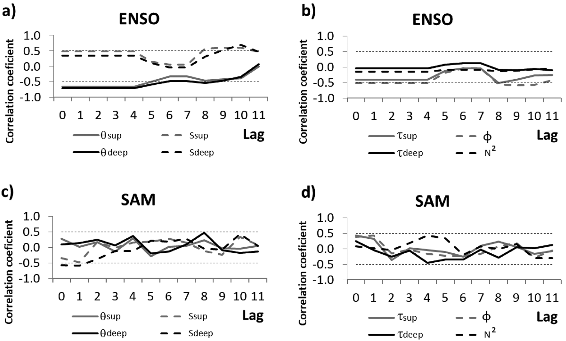
Fig. 10.Cross-correlation coefficients between monthly ENSO and SAM with hydrographic parameters inside the NA polygon. Each lag corresponds to one month. Horizontal dotted black lines represent confidence bounds at 95%.
A previous (up to 4 or 5 months) positive (negative) phase of ENSO leads to a colder (warmer) water column and more saline (fresher) surface layer in NA (Fig. 10a). Also, significant correlations with θ (in deeper waters) and S were found from lag 8. Month lags in the response of these correlations appears reasonable compared with previous studies in the region (e.g. Ruiz Barlett et al. Reference Ruiz Barlett, Tosonotto, Piola, Sierra and Mata2018). Additionally, ENSO is negatively linked with surface τ and the ϕ of water column (Fig. 10b). On the other hand, a negative and significantly rank correlation (in lag 0 and 1) were obtained between SAM and S in deeper waters (Fig. 10c). Significant relationships between ENSO with thermohaline parameters and SAM index with S in deeper waters are in agreement with those reported a little further from the FG by Schloss et al. (Reference Schloss, Abele, Moreau, Demers, Bers, González and Ferreyra2012). Also, these authors reported a positive relation between SAM (with no lag) with sea surface temperature, wind intensity, total particulate material and chlorophyll. Additionally, no significant correlations were found between SAM versus θ and τ of the NA water column. On another hand, ENSO seems to have more impact on PC than SAM as shown in previous studies over the WAP region (e.g. Stammerjohn et al. Reference Stammerjohn, Martinson, Smith and Yuan2008, Clem & Fogt Reference Clem and Fogt2013, Ruiz Barlett et al. Reference Ruiz Barlett, Tosonotto, Piola, Sierra and Mata2018). Therefore, the influence of ENSO conditions could also affect the water structure of this region.
In general, larger easterly winds on the study area are associated with a negative SAM, as well as larger westerlies to a positive SAM (Schloss et al. Reference Schloss, Abele, Moreau, Demers, Bers, González and Ferreyra2012). Also, they reported an opposite and lower relationship with ENSO. This relation can be noticed in Fig. 2 and is fully studied, on the Antarctic Peninsula region. Both El Niño and negative SAM phases have been related to easterly anomalies (e.g. Yuan Reference Yuan2004, Marshal et al. Reference Marshall, Orr, van Lipzig and King2006). During months in which easterlies were predominant in the study region, there was a decrease of water temperature due to air cooling (as the 2010 summer), these conditions favoured upwelling events of deep water from Maxwell Bay (Klöser et al. Reference Klöser, Ferreyra, Schloss, Mercuri, Laturnus and Curtosi1994, Roese & Drable Reference Roese and Drable1998).
Summers 2010 and 2016 (El Niño conditions)
Summers 2010 and 2016 were characterized by colder anomalous ϕ and significant snow precipitation, with a positive ENSO phase (El Niño) over the equatorial Pacific (Fig. 2). Low wind velocities were recorded during this period (except in February 2016). Consequently, colder and less freshwater input led to the low vertical stratification observed in the PC water column (Table II). Cold Tair anomalies were present during both previous winter and spring seasons (Fig. 9a). After very cold winters (with high SIC), the late ice melt and the consequent stratification of the surface layer before the FG ice is discharged into the cove have enhanced strong bloom events (e.g. Schloss et al. Reference Schloss, Abele, Moreau, Demers, Bers, González and Ferreyra2012, Reference Schloss, Wasilowska, Dumont, Almandoz, Hernando and Michaud-Tremblay2014, Kim et al. Reference Kim, Ducklow, Abele, Ruiz Barlett, Buma and Meredith2018) and inhibited the growth of macroalgae (Klöser et al. Reference Klöser, Ferreyra, Schloss, Mercuri, Laturnus and Curtosi1993). Chlorophyll positive anomalies in PC waters during El Niño conditions were found in January 2010 (Schloss et al. Reference Schloss, Wasilowska, Dumont, Almandoz, Hernando and Michaud-Tremblay2014) and spring–summer of 2015–16 (Kim et al. Reference Kim, Ducklow, Abele, Ruiz Barlett, Buma and Meredith2018). After those El Niño summers, the two longest winter and spring seasons with anomalously warm Tair and less SIC can be observed over the period 2009–17 (see Fig. 9a & b).
Air and surface waters result in significantly colder temperatures during summer 2010 for the 8-summers study period. This very cold condition on Carlini Station was reported by other authors (e.g. Bers et al. Reference Bers, Momo, Schloss and Abele2012, Deregibus et al. Reference Deregibus, Quartino, Campana, Momo, Wiencke and Zacher2016), who also indicate negative temperature anomalies since early winter of 2009. El Niño conditions in phase with negative SAM enhanced the cold air and easterly winds over PC (Schloss et al. Reference Schloss, Wasilowska, Dumont, Almandoz, Hernando and Michaud-Tremblay2014). These authors made several analyses of this event. This summer recorded one of the lowest τ values in the surface layer of the inner cove for the study period (Fig. 6c). The persistence of this event led to less intense glacial melting than previous years and therefore, lower total suspended particulate matters (Bers et al. Reference Bers, Momo, Schloss and Abele2012). Deregibus et al. (Reference Deregibus, Quartino, Campana, Momo, Wiencke and Zacher2016) affirm that a less turbid water column could enhance macroalgal productivity.
Conversely, in summer 2016, a positive SAM counteracts the colder El Niño conditions over the study region, associated with more frequent westerlies and south-westerlies (Fig. 2). Consequently, the atmosphere and water were slightly warmer than summer 2010. Furthermore, low salinity in deep waters during January 2016 associated with a cold water column (see Fig. 6 g & h) could be related to the warm air conditions during the beginning of the month (Fig. S2) and relatively high Tair observed in previous December (not shown). These results are in agreement with other studies which show a positive feedback effect when a positive (negative) ENSO and a negative (positive) SAM phase are observed on the Antarctic Peninsula region (e.g. Fogt et al. Reference Fogt, Bromwich and Hines2011, Ruiz Barlett et al. Reference Ruiz Barlett, Tosonotto, Piola, Sierra and Mata2018). During winter 2016, is attenuated El Niño influence and only positive SAM phase was reflected by warm air conditions (Fig. 9). As a result, sea ice showed the lowest anomalous extent and fastest retreat over the study area, as well as the warmer surface waters around most of Antarctica (Stuecker et al. Reference Stuecker, Bitz and Armour2017). However, the SAM sign changed to negative during the following spring and summer, associated with low intensity winds (Fig. 2). This situation possibly promoted the relatively high stratification and slight stability of the PC water column in summer 2017 (Table II), also was reported in the nearby Maxwell Bay and related with a phytoplankton bloom (Höfer et al. Reference Höfer2019).
Summers 2011 and 2012 (La Niña conditions)
La Niña and positive SAM predominant conditions were present during the summers of 2011 and 2012 (Fig. 2). During these months, stronger westerly winds were more frequent on PC (except February 2012, a negative SAM month). The advection of relatively moist and warm air resulted in the warmest, rainiest (mainly in February) and windiest summers in the studied period. This result is in agreement with previous authors (e.g. Yuan Reference Yuan2004, Stammerjohn et al. Reference Stammerjohn, Martinson, Smith and Yuan2008, Fogt et al. Reference Fogt, Bromwich and Hines2011). Also, warmer temperatures in the water column (negative and positive linked with ENSO and SAM, respectively) were found during these months. Thus, warmer negative ENSO conditions will enhance particulate material increases in the PC water column. This is related with the negative significant link observed between ENSO and τ in the surface layer of NA waters (Fig. 10b). Additionally, Garcia et al. (Reference Garcia, Hoffmeyer, López Abbate, Barría de Cao, Pettigrosso and Almandoz2016) reported a higher microzooplankton total biomass and differences in its composition between the cold summer 2010 and 2011, summers strongly influenced by El Niño or La Niña predominant conditions respectively according to our study.
Between winter–spring 2010, positive Tair anomalies during La Niña conditions were in phase with a strong positive SAM. A critical attenuation in the SAM index was observed during December and January and a relatively normal Tair was present on PC (Fig. 9). This period is characterized by decreased sea ice growth, more sea ice melt and water column stability in the spring, which led to low phytoplankton growth and accumulation in the spring/summer (e.g. Stammerjohn et al. Reference Stammerjohn, Martinson, Smith and Yuan2008, Kim et al. Reference Kim, Ducklow, Abele, Ruiz Barlett, Buma and Meredith2018). Also, the largest accumulated rainfall and the strongest mean winds were found during February 2011, a remarkable warm month in the study period (Fig. 2).
A strong anomalous cold winter in 2011 during negative SAM and neutral ENSO months accompanied by increased SIC was present in the PC region (see Fig. 9). Following months (spring–summer) characterized by negative ENSO in phase with positive SAM index showed warmer Tair. This early summer led to premature meltwater input to the cove and therefore, the minimum monthly mean of S obtained in January 2012 in the entire water column, as discussed earlier. In addition with the high rainfall in the following month, could lead to great freshwater input and therefore, explain the lowest S and highest τ values observed during this summer (Table II) indicating large contributions of meltwater creeks and glacier discharge. In consequence, high stratification and stability values were obtained, particularly in January, due to lower winds intensity than those recorded in summer 2011.
Summer 2015 (positive SAM)
Late spring 2014 and early summer 2015 were characterized by a positive SAM and strong westerlies mean conditions (see Fig. 2). However, relatively cold air was present on PC, probably related to a neutral ENSO phase. Consequently, a low stratified water column could be associated with cold and more saline waters during January 2015, although a pronounced thermocline was distinguished (see Fig. S4). The following month was warmer both in air and water column, probably related to a stronger positive SAM, which favours glacier meltwater contributions (see Figs 2 & 6). This result is in accordance with Falk et al. (Reference Falk, López and Silva-Busso2018), who reported a decreasing discharge of summer meltwater from a model output between 2011 and 2014, and an increase in 2015. In consequence, low S was found in the PC water column during February 2015, which was, also, reported in the nearby Admiralty Bay (Lima et al. Reference Lima2019). Furthermore, a high monthly mean of the vertical stratification was found in the NA water column.
Summary and conclusions
In this study, we characterized the atmospheric and oceanographic parameters of PC during eight summers (2010–17) in order to analyse the temporal variability and relate it with SIC and two main modes of climate variability, as ENSO and SAM. Oceanographic parameters in the cove showed large variations both on monthly and interannual time scales associated with atmospheric forcings and input of surrounding waters. Significant differences were found between the surface and the deepest layers in two zones of inner PC: in front of Carlini Station and closer to the FG. Also, vertical stratification parameters were positive (negative) linked to air and water temperature and turbidity (salinity and density) in the first meters of the water column near the glacier. Furthermore, in deeper waters, thermohaline and stratification parameters were significantly correlated. Finally, different conditions were presented both in the air and water systems between two consecutive months (January and February) during the summers.
Significant differences in the water structure between the two study areas were only found in turbidity. The latter, more influenced by large freshwater inflows from meltwater creeks, cascades and glacier detachments (and a decreasing subglacial meltwater), has a large influence in the interannual variability of salinity and turbidity. High mean rainfall during warm summers can lead to more terrigenous sediment runoff and therefore, more turbid waters in the cove. Some of these results agree with those obtained in the cove by previous authors. Also, high turbidity values were detected into deep waters near the glacier, principally during the summers of 2013 and 2014. These could be due to resuspended soft sediment associated with glacial discharge events and mixing by katabatic winds. This “New Area” has been quite studied in recent years by several groups because it is a recent ice-free zone and has been gradually colonized by benthos and algae. Therefore, it is the key to determine the dynamics and origin of the contributions of water and sediment into the water column in the vicinity of the glacier front.
The summer mean air conditions of the study period were significantly colder than the previous 1991–2009 at Carlini Station. However, the FG has retreated towards the coastline in recent years and only 530 m of glacier still continues to be on PC waters. In consequence, some typical processes that occur into the waters near the glacier front in a fjord, such as the contribution of waters leaving the glacier at depth, would appear to be no longer present or significant in PC. Therefore, oceanographic parameters in the cove show large variations both on monthly and interannual time scales associated with atmospheric forcing. Here, the local meteorological influence is more important than in waters of other fjords, where the main forcing is the temperature of the seawater that penetrates the cove. The FG retreat due to atmospheric factors, such as the increase in rainfall events, could lead to a significant increase in changes observed in the Potter system in recent years. Determining the dynamics of the PC stream system and the temporal variability in the contribution of meltwater and suspended material is of vital importance to understand the functioning of marine ecosystems.
A negative significant correlation was found between SIC and air temperature with a delay of at most 1 month and with deeper waters near the FG of four months. A warm winter–spring leads to less SIC and an early breaking as can be seen during 2010 and 2016. After the sea ice retreat, the water column is heated and wind-induced mixing before the meltwater contribution. Consequently, a warmer and fresher mean water column during summer is obtained, particularly observed in 2012 due to early summer conditions. On the contrary, a cold Tair anomaly after a warm winter–spring could explain the most saline deep waters found during summer 2017.
In order to further understand connections between local parameters at PC and ENSO/SAM modes, significant cross-correlations were obtained. A positive phase of ENSO (El Niño) is associated with colder conditions over the study area and the largest SIC events during winter, or eventually during the previous one. On the contrary, after El Niño, winter–spring periods were noticeably warm with the lowest observed SIC, as discussed in the previous paragraph. Significant correlations were obtained between ENSO and Tair with lag no longer than 1-month and water temperature with lags as long as four months, reflecting the different time of response between the atmosphere and the ocean. Additionally, the beginning of the ENSO event in the Pacific (in autumn), and their influence in the SIC, are linked with other summer oceanographic properties like salinity (vertical stratification) and surface turbidity. SAM, instead, shows no significant correlation with local parameters beyond lag 1. In consequence, ENSO influence on the PC region could be more important than SAM in longer timescales.
Summers of 2010 and 2016 were under the influence of a positive ENSO phase. Easterly and southerly winds were predominant, producing colder conditions and high percentage of snowfall on PC. As a consequence, a cold water column and upwelling events could be more recurrent. These conditions were more pronounced during summer 2010 (negative SAM phase) than summer 2016, since a positive SAM phase counteracted El Niño effects. Conversely, 2011–12 was a period characterized by simultaneous in-phase negative ENSO (La Niña) and positive SAM phases, which led to more westerly winds. Warmer temperatures and more precipitation (in February) were observed, and therefore, the glacier surface melting favours the freshwater and terrigenous sediments runoff input to the PC system. Consequently, a fresher and more turbid surface layer was present, particularly, in January 2012. Thus, simultaneous in-phase ENSO and SAM (with opposite sign) phases should enhance their effects on the cove, in agreement with previous studies in the region. Finally, warm air and strong westerlies mean conditions during February 2015 are related to a positive SAM phase. In consequence, warm and fresh waters led to a vertically stratified water column.
Characterizing the oceanographic processes associated with the distribution of the biological population in the water column is crucial to understand how they are affected by climate change. The link between the meteorological/climatological conditions at the time of the measurements in the water column will allow having a better understanding of the PC system and reinforcing the results obtained in this work. To confirm the significant relationship between the interannual changes in the hydrographic properties, biological and environmental modifications of the cove and the climate variability modes, it is necessary to continue collecting high-quality hydrographic data. The deployment of moorings capable of detecting subtle changes in the characteristics of the water column with an increased sampling frequency would also improve the description of PC dynamics. To address these issues, long-term observations in the Maxwell Bay (linked to PC) and numerical models may also be needed.








 You have
Access
Introduction
Fjords are estuaries that have been or are being modified by neighbouring glaciers. They are a transition zone between land and ocean and therefore its waters present strong gradients in their physico-chemical characteristics. The physical properties of seawater such as temperature, salinity, density and turbidity are important in the diversity of oceanic processes. Glacial melting during summer seasons produces the input of fresh water and terrigenous suspended particulate matter to the ocean by surface and subglacial erosion and meltwater flows (e.g. Monien et al. Reference Monien, Monien, Brünes, Widmer, Kappenberg and Busso2017, Meredith et al. Reference Meredith, Falk, Bers, Mackensen, Schloss and Ruiz Barlett2018). This leads to the formation of sediment plumes characterized by low salinity (and therefore, less dense waters) from the glacier to waters outside the bays (e.g. Syvitski Reference Syvitski1989, Klöser et al. Reference Klöser, Ferreyra, Schloss, Mercuri, Laturnus and Curtosi1993, Rodrigo et al. Reference Rodrigo, Giglio and Varas2016). The location of these fresher and more turbid thin layers can vary significantly in space and time due to variations in glacial runoff or wind activity (Hass et al. Reference Hass, Kuhn, Monien, Brumsack and Forwick2010). The stratification level is determined by the balance between diluted water discharge, buoyancy flux and physical processes such as wind-induced mixing and tide which homogenizes the water column (Syvitski Reference Syvitski1989). The contribution of suspended material to the fjord is greater when the stratification is best developed (Syvitski Reference Syvitski1989). Surface meltwater plumes stabilize the water column and therefore favour the development of summer chlorophyll blooms (Höfer et al. Reference Höfer2019).
The Western Antarctic Peninsula (WAP; Fig. 1a) is the region with the largest increase in near-surface air temperature (Tair; +3.7 ± 1.6°C century-1) during the mid-20th century (e.g. Vaughan et al. Reference Vaughan, Marshall, Connelley, Parkinson, Mulvaney and Hodgson2003). This warming has been associated with a diversity of regional changes: accelerated glacier retreat (Rignot et al. Reference Rignot, Jacobs, Mouginot and Scheuchl2013), precipitation increase (Uotila et al. Reference Uotila, Lynch, Cassano and Cullather2007) and strong meltwater discharge into the coastal zone (Hass et al. Reference Hass, Kuhn, Monien, Brumsack and Forwick2010). The atmospheric warming in the WAP has shown marked variability and periods of superposed cooling, e.g. Tair trend inversion since the late 1990s associated with greater east-south-easterly winds (Turner et al. Reference Turner2016).
Maps showing location of a. King George (25 de Mayo) Island, South Shetland Islands, and b. Potter Cove (PC). c. Location of hydrographic stations (black dots) in the inner PC. Stations were separated in two basins: in front to Carlini Station (Carlini Area: CA) and closer to the Fourcade Glacier (New Area: NA), represented by the dashed polygons. The white contour polygon represents the locations of profiles selected for calculating averages within NA. The glacier area retreated between 1956 and 2018 (coastline) is shown with colour lines (modified from Rückamp et al. Reference Rückamp, Braun, Suckro and Blindow2011). The glacier front in the water (December 2018) is marked in light blue. The shaded background displays the bottom topography (scale at right) in each panel. CAMS: Campbell Automatic Meteorological Station.
Two predominant modes of large-scale climate variability affect the Southern Ocean, particularly the Antarctic Peninsula region: the Southern Annular Mode (SAM; e.g. Thompson & Wallace Reference Thompson and Wallace2000) and the El Niño–Southern Oscillation (ENSO; e.g. Yuan Reference Yuan2004). The SAM is the main mode of variability of the Southern Hemisphere High Latitudes. It is directly associated with mid-latitude wind patterns, since it represents the exchange of atmospheric mass between lower and higher latitudes. This can be quantified by an index calculating the difference of zonal mean sea level atmospheric pressure between 40°S and 65°S latitudes, which fluctuates between positive and negative phases (Thompson & Wallace Reference Thompson and Wallace2000). This index presents a positive trend since the 1960s associated with an increase of westerly winds and the consequent air warming over the WAP (e.g. Marshall et al. Reference Marshall, Orr, van Lipzig and King2006). The ENSO, instead, is the main oscillation of the climate system on Earth, characterized by large-scale atmospheric pressure and sea surface temperature fluctuations in the equatorial Pacific affecting high latitudes of the Southern Hemisphere (Yuan Reference Yuan2004). During the negative phase of the ENSO (La Niña), a cyclonic circulation anomaly is located on the WAP, increasing the strength and frequency of north-westerly winds (Yuan Reference Yuan2004). This can lead to warmer air and water temperatures along the WAP, while the opposite pattern may occur during El Niño events (e.g. Stammerjohn et al. Reference Stammerjohn, Martinson, Smith and Yuan2008, Ruiz Barlett et al. Reference Ruiz Barlett, Tosonotto, Piola, Sierra and Mata2018). During the latter, warmer temperatures and less extent and duration of sea ice cover (SIC) are presented in the South Pacific while the inverse response is observed in the South-west Atlantic (Yuan Reference Yuan2004, Stammerjohn et al. Reference Stammerjohn, Martinson, Smith and Yuan2008). Fogt et al. (Reference Fogt, Bromwich and Hines2011) found that when SAM and ENSO are out phase (in phase), the ENSO teleconnection to the South Atlantic is stronger (weakened or absent). Conversely, the opposite response pattern is presented in the South Pacific region.
The Potter Cove system
Potter Cove (PC) is a semi-enclosed body of water located on King George (25 de Mayo) Island, South Shetland Archipelago (Fig. 1b). The area of the cove is approximately 7 km2 and its main axis has a SW–NE direction. The western edge is open to Maxwell Bay (Bahía Guardia Nacional). The northern and eastern coasts of PC are bounded by the Fourcade Glacier (FG; Fig. S1) while the southern coast is a beach of coarse sand and gravel (Wölfl et al. Reference Wölfl, Lim, Hass, Lindhorst, Tosonotto and Lettmann2014). Predominant winds are from the north-west and east (Klöser et al. Reference Klöser, Ferreyra, Schloss, Mercuri, Laturnus and Curtosi1994, Roese & Drabble Reference Roese and Drable1998, Schloss et al. Reference Schloss, Abele, Moreau, Demers, Bers, González and Ferreyra2012). In general, a cyclonic circulation allows the renewal of the PC waters that come from the northern side and leave through the southern sector. Furthermore, a vertical circulation cell exists with wind intensities higher than 5 m s-1, producing upwelling (downwelling) in the eastern edge of the cove during eastern (western) wind events (Roese & Drabble Reference Roese and Drable1998). Roese & Drabble (Reference Roese and Drable1998) postulated that tides are mixed with semidiurnal predominance and low-intensity tide currents.
The South Shetland Islands have a relatively moderate and humid climate compared to the PA region due to predominant westerly winds, its lower latitude and sea moderating effects (Schloss et al. Reference Schloss, Abele, Moreau, Demers, Bers, González and Ferreyra2012). Consequently, break and surface thinning of the coastal ice shelves have led to the retreat of coastal marine and tidewater glaciers (e.g. Rignot et al. Reference Rignot, Jacobs, Mouginot and Scheuchl2013). The low salinity surface layer in PC is formed during the meltwater season (summer) by the input of cascading glacial melt and melting of floating ice blocks and brash ice (that could also enter from the Maxwell Bay). Also, the southern coast presents a stream system during this season conditions (Fig. S1), with one creek due to precipitation (Matías Creek) and three due to glacial meltwater, which discharge surface and subterranean fine sediments (mainly silt) into the cove (Wölfl et al. Reference Wölfl, Lim, Hass, Lindhorst, Tosonotto and Lettmann2014, Monien et al. Reference Monien, Monien, Brünes, Widmer, Kappenberg and Busso2017). Of the latter, one has been called Potter Creek and the other two we have named unofficially “Oscar” and “Carlini” creeks. Monien et al. (Reference Monien, Monien, Brünes, Widmer, Kappenberg and Busso2017) estimated a meltwater discharge transport of 2–4 10-4 tons yr-1 of suspended particulate matter into the surface layer of the cove. Thus, during summer the PC circulation pattern is dominated by surface plumes of turbid, relatively warm meltwater that flow out of the fjord (e.g. Klöser et al. Reference Klöser, Ferreyra, Schloss, Mercuri, Laturnus and Curtosi1993, Reference Klöser, Ferreyra, Schloss, Mercuri, Laturnus and Curtosi1994) and depends on the stratification level controlled by freshwater input (Syvitski Reference Syvitski1989).
The annual mean Tair in the Jubany meteorological station, at Carlini (former Jubany) station, increased 0.66 °C between 1991 and 2009 (Schloss et al. Reference Schloss, Abele, Moreau, Demers, Bers, González and Ferreyra2012). These authors reported increasing sea surface temperature and total suspended particulate material in PC waters during this period, influencing a remarkable 20 km2 retreat of the FG (Fig. 1c) and significant loss of its glacier cover since the 1950s (Rückamp et al. Reference Rückamp, Braun, Suckro and Blindow2011). The FG has been a retreating tidal glacier (Rückamp et al. Reference Rückamp, Braun, Suckro and Blindow2011) that recently switched to a land terminating glacier, and its melting is strongly associated with local air temperature (Falk et al. Reference Falk, López and Silva-Busso2018, Meredith et al. Reference Meredith, Falk, Bers, Mackensen, Schloss and Ruiz Barlett2018). Subglacial meltwater inputs from the FG, mainly from the north-east coastline (Klöser et al. Reference Klöser, Ferreyra, Schloss, Mercuri, Laturnus and Curtosi1993, Reference Klöser, Ferreyra, Schloss, Mercuri, Laturnus and Curtosi1994), have decreased in recent years. Therefore, the meltwater and freshening dynamics are now mainly driven by surface runoff (Meredith et al. Reference Meredith, Falk, Bers, Mackensen, Schloss and Ruiz Barlett2018). The periodic ice supply is affecting benthic communities in shallow waters near the glacier, while glacier retreat generates new ice-free areas available for colonization (e.g. Sahade et al. Reference Sahade2015, Deregibus et al. Reference Deregibus, Quartino, Campana, Momo, Wiencke and Zacher2016). Several studies have analysed physico-chemical and biological processes within PC waters (e.g. Klöser et al. Reference Klöser, Ferreyra, Schloss, Mercuri, Laturnus and Curtosi1993, Reference Klöser, Ferreyra, Schloss, Mercuri, Laturnus and Curtosi1994, Deregibus et al. Reference Deregibus, Quartino, Campana, Momo, Wiencke and Zacher2016) and their relation with the climate variability, including ENSO and SAM (Bers et al. Reference Bers, Momo, Schloss and Abele2012, Schloss et al. Reference Schloss, Abele, Moreau, Demers, Bers, González and Ferreyra2012, Reference Schloss, Wasilowska, Dumont, Almandoz, Hernando and Michaud-Tremblay2014, Kim et al. Reference Kim, Ducklow, Abele, Ruiz Barlett, Buma and Meredith2018).
The aim of this article is to analyse the interannual variability of waters within the inner area of the PC during summers (January to February) from 2010 to 2017 and its connection with climate change. Studying the oceanographic processes that affect the cove waters has a vital importance to characterize and evaluate changes in the marine ecosystem. In order to study how physical characteristics of the Potter system can be affected by the contribution of melting water and glacier detachments, several oceanographic parameters (water temperature, salinity and turbidity) sampled in two regions of PC, near and away from the glacier front, plus atmospheric variables (Tair, precipitation and wind conditions), as well as monthly SIC data, were analysed. Then, the temporal variability in 3-layers of the area closer to the glacier was studied. Finally, we carried out a combined analysis of ENSO and SAM together with the hydrographic and atmospheric changes in the PC observed from 2009 till 2017.
Materials and methods
Meteorological and sea ice cover data
A Campbell Automatic Meteorological Station was installed each summer (January to February) from 2010 to 2017 near Elephant Point (62°14′16.1″S, 58°40′44.4″W), over the south-west extreme of the PC (Fig. 1c), a site near the mouth of the cove which is less affected by orography. Sensors of surface Tair and wind were placed at 8 m above sea level and their measurement rate was set at a frequency of 10 minutes. Time series of mean daily Tair and accumulated monthly wind roses during the eight summers of this period are shown in Fig. S2 and Fig. S3, respectively. Missing data were interpolated with daily means of the Jubany meteorological station (3-hourly frequency data) from the Servicio Meteorológico Nacional (SMN), the National Weather Service of Argentina. Also, daily accumulated precipitation was obtained from the SMN. Precipitation values on daily positive (negative) Tair are considered as rainfall (snow). Then, monthly means for each parameter and monthly predominant wind direction were obtained.
The area-averaged SIC fraction data were obtained from the MERRA-2 model M2TMNXFLX v5.12.4, available at https://giovanni.gsfc.nasa.gov/giovanni/ (GMAO 2015), which provides monthly time series with a 0.5° x 0.625° resolution. In this study we used the monthly mean of SIC between January 2009 and December 2016 at 58°45'W–58°36'W and 62°12'S–62°15'S.
Bathymetry data
The bathymetry transects were performed in PC with an integrated Garmin Echo sounder-GPS system onboard pneumatic boats during the summers 2010–12. Data were corrected by tide prediction and they were referred to mean sea level. Bottom marine topography (Fig. 1c) was obtained using the Kriging interpolation method. The coastline of the cove and south-west coast of the island near Carlini Station was measured with a Garmin GPS. A shallow sill (~30 m) separates the inner (55 m maximum depth) and outer (~200 m depth) areas (Klöser et al. Reference Klöser, Ferreyra, Schloss, Mercuri, Laturnus and Curtosi1994). In turn, the inner PC can be divided into two basins by a sill of about 25 m depth, which is located approximately in the western limit that had the glacier in 1956 (Rückamp et al. Reference Rückamp, Braun, Suckro and Blindow2011). The retreat of the FG resulted in a sea ice-free zone of 0.97 km2 from 1997 to 2010. Between February 2010 and December 2018, the FG has retreated 0.042 km2 in the east end and only 530 m of its cover is in the water in late 2018 (Fig. 1c).
Hydrographic data
The measurements of the physico-chemical parameters of the sea water column were conducted using a SBE 19plus V2 CTD (Conductivity, Temperature and Depth), with an auxiliary ECO NTU turbidity sensor. Sampling was carried out from pneumatic boats (wind conditions < 20 knots) during summer (January and February) over an 8-year period (2010–17). An oceanographic winch was used to reach the bottom waters in the inner cove (~55 m deep), except in 2010, 2012 and 2016, when the measurements were made in the first 30 m. We excluded observations with less than 1 m depth in order to homogenize the initial value and filter surface effect in CTD sensors such as wave rugosity and Tair. CTD data were processed using SBE Data Processing software. Then, potential temperature (θ), salinity (S) and potential density anomaly (σ) were calculated using the International Thermodynamic Equation of Seawater-2010 (TEOS-10; IOC et al. 2010), with precisions of 0.001°C in temperature and 0.0003 in salinity.
We considered two areas in the inner PC: one in front of the scientific station, Carlini Area (CA), and the other closer to the FG, New Area (NA), which is an ice free area due to glacier retreat since the 1950s. Schloss et al. (Reference Schloss, Abele, Moreau, Demers, Bers, González and Ferreyra2012) compared two stations far and near the FG in PC over 19 years. As a consequence of the glacier retreat, CA, which we compare with NA, coincides with the area previously near the FG used by these authors. Summer mean profiles and standard deviations of hydrographic properties were obtained to compare the vertical thermohaline structure in both areas. To study the temporal variability, we selected stations located in the central area of NA (Fig. 1c), to minimize spatial variability. The water column was separated in three depth strata: 1–5 m (surface water), 5–10 m (approximately the pycnocline location) and > 10 m (deep water). For each profile, we calculated mean values of the oceanographic properties for the three selected layers. Then, monthly means and standard deviations were estimated. In order to quantify the vertical stratification of the water column, Simpson's parameter (ϕ; as in Simpson et al. Reference Simpson, Allen and Morris1978) from each profile was calculated, and to analyse the stability conditions, Brunt-Väisälä or buoyancy frequency (N2; Millard et al. Reference Millard, Owens and Fofonoff1990) was determined. Both equations are presented in Supplementary Material as Eq. S1 and Eq. S2, respectively. Finally, mean and maximum monthly values were estimated for the analysed 8-summer period.
Modes of climate variability
Monthly means of the SAM index were obtained from the British Antarctic Survey (BAS; https://legacy.bas.ac.uk/met/gjma/sam.html). The monthly Bivariate ENSO Timeseries (BEST) Index (Smith & Sardeshmukh Reference Smith and Sardeshmukh2000) obtained from the Climate Diagnostics Center (CDC; http://www.cdc.noaa.gov/people/cathy.smith/best/) was, also, used in this study. We selected the BEST index to determine ENSO events because both the atmospheric processes and the oceanic components, i.e. the Southern Oscillation Index and Niño 3.4 Index, are combined.
ANOVA and correlations
Non-parametric Kruskal-Wallis one-way ANOVA test was used to compare the daily means of the oceanographic parameters between the two areas (CA and NA) and between the surface and the deepest layer (> 10 m) in each area. Also, an ANOVA test followed by a Bonferroni post-test was used to compare monthly and interannual means in the central region of NA. The test was applied to monthly means of Tair and SIC for a whole year, to summer Tair and precipitation (Tair ≥ 0 °C) and oceanographic variables. Cross-correlations were made to determine Kendall's correlation coefficients. These correlations were carried out between monthly means of Tair, SIC and climate variability modes (ENSO and SAM) as well as with the hydrographic averages of the shallow and the deepest NA layers. The significance level was P < 0.05 for correlations with oceanographic parameters and P < 0.01 in remaining cases.
Results
Meteorological summer conditions in Carlini Station (2010–17)
January and February monthly mean of Tair show high monthly and interannual variability during the period 2010–17 (Fig. 2 and Table S1). Summer 2011 was warm while 2010 and 2014 were cold summers (Bonferroni ANOVA, P < 0.05). Monthly Tair means for 2010–17 summers are 1.14 ± 0.39°C (January) and 1.23 ± 0.93°C (February), statistically not different. The maximum daily Tair (9.66°C) was recorded on 1 January 2016 while the minimum (-6.24°C) was observed on 9 February 2014. February 2011 was the warmest and rainiest month with the highest mean wind intensity and westerlies frequency. Alternatively, during predominant easterlies in February 2010 and southerlies in January 2014, respectively, colder summers were observed with a fraction of precipitation in negative daily temperature (snow) conditions.
Monthly values at Carlini Station of a. mean near-surface air temperature (Tair; represented by diamonds) with one standard deviation (vertical bars), b. accumulated precipitation (PP) of rainfall (Tair ≥ 0 °C) and snow (Tair < 0 °C) and c. percentage of occurrence of monthly predominant wind direction from east (E), south-east (SE), south-west (SW) and west (W). Diamonds represent wind intensity monthly means associated with predominant directions. Different letters represent significant differences (ANOVA test followed by a Bonferroni post-test, P < 0.05) between months during the eight-summer period for a. Tair and b. rainfall. Shared letters indicate non-significant differences. SAM and BEST (ENSO) monthly index during January and February are shown above panel a.
Hydrographic properties of Potter Cove
The interannual mean θ profiles do not present significant differences between CA and NA (Fig. 3 and Table I), although the Kruskal-Wallis ANOVA showed significant differences between shallow and deeper waters within each area. Air temperature-induced θ conditions originate at the water surface and propagate downward into the water column by wind-induced mixing. Thus, warmer summers are visible throughout the entire water column (< 50 m deep). The water column was warmer in summer 2012 while the coldest waters were observed in 2010. The maximum θ range in the PC waters resulted between 0.047 and 2.864°C, with its maximum value recorded in surface waters on 13 February 2015. In fact, 2015 presented the highest θ variability, while the most homogeneous profiles were obtained in 2010. When comparing January and February each summer (Fig. S4), some interesting aspects deserve to be pointed out. In general, θ decreases with depth although some profiles presented warming from the surface to a subsurface maximum and then the waters become colder as the depth increases (February 2011, 2012 and 2016). During summers of 2011, 2013 and 2015, θ profiles for February were warmer than January. The lowest mean θ was obtained in January 2015, although they were calculated from a daily single profile. At the time of the measurement (8 January) and in the previous hours, the wind was predominant from the glacier direction (easterlies), which resulted in Tair values lower than -1.5°C. In January 2016, the water column was more stratified and warmer than in February, although few sampling days were carried out during this summer due to adverse weather conditions.
Mean potential temperature (θ) profiles a., b. in the CA, and c., d. NA for the period 2010–13 and 2014–17, respectively. Horizontal bars represent one standard deviation around the mean of certain chosen depth. Vertical dashed line represents 1°C.
Upper panel: Results of Kruskal-Wallis one-way ANOVA comparing areas (CA and NA) and water layers in PC. Lower panel: Significant correlations (at 95% in italic and 99% in bold) between hydrographic parameters into the black polygon in NA.
The structures of the mean S profiles between CA and NA obtained in the deepest layer were more similar to each other than those of the shallower layer (Fig. 4). However, only the difference between surface and deeper layers within each area are statistically significant (Table I). The stratification in the first meters of the water column shows the freshwater input from FG and glacio-fluvial creeks, more visible in NA during summers of 2012 and 2013. The mean θ profiles in 2012 and 2015 (> 4 m) resulted fresher compared to the rest of summers in both areas. January was less saline than February in 2010, 2012 and 2017 (Fig. S5). The θ-S diagrams in Fig. S6 shows high inter-annual and summer variability of the thermohaline properties in the PC water column. Low S was observed in surface waters both in relatively warm and cold conditions, since changes in density layers in fjords like PC are mainly affected by variations in S due to glacier freshwater inputs during summer.
Mean salinity (S) profiles a., b., e., f. in the CA, and c., d., g., h. NA for the period 2010–13 and 2014–17, respectively. Horizontal bars represent one standard deviation around the mean of certain chosen depth. Upper panel represents 1–10 m depth layer and lower panel represents deeper than 10 m. Note the different scales between both panels. Vertical dashed line represents S of 33 (upper panel) and 34 (lower panel).
Mean turbidity (τ) profiles show increasing values in the surface layer of the CA (Fig. 5a & b). Instead, high interannual variability is visibly in the NA (Fig. 5c & d). Here, surface τ values nearly to 30 NTU were reached several times (Fig. S7). On the other hand, deeper waters near the mouth of the inner cove showed very low turbid values, although were relatively higher during 2012 and 2017 (Fig. 5e & f). In general, τ values decrease with depth. However, during some summers (mainly 2013 and 2014) high τ values in deeper waters (>10 m) were recorded by several CTD profiles located in the PC eastern edge (Fig. 5 g & h). These turbid deep waters were present both in January and February (Fig. S7). In particular, 2014 reached values greater than 10 NTU in waters deeper than 20 m. Turbidity shows significant differences (P < 0.05) between both areas and shallow and deeper waters (Table I). Finally, high τ values were recorded both during low and relatively high S conditions (Fig. S8), reaching a maximum of 29.25 NTU on 25 January 2010 in the surface layer near the glacier. During January 2012 extremely low surface S values were found in PC waters compared to other observations obtained during similar maximums τ conditions (~30 NTU). It may be associated with higher contribution of freshwater input from the glacier because of relatively warm air conditions on the cove and melting of floating ice blocks. Correlations between S and τ in the water column will be explored in the Discussion.
Mean turbidity (τ) profiles a., b., e., f. in the CA, and c., d., g., h. NA for the period 2010–13 and 2014–17, respectively. Horizontal bars represent one standard deviation around the mean of certain chosen depth. Vertical dashed line represents τ of 10 (upper panel) and 2 NTU (lower panel).
Interannual variability of hydrographic properties in the New Area (NA)
For each of the 3 layers in which the central region of the NA (see Fig. 1c) was vertically divided, we found significant differences between monthly mean hydrographic properties during the 8-summer period, from 2010–17. Summer θ in surface waters (1–5 m layer) resulted significantly colder in 2010 and warmer in 2011 and 2012 (Bonferroni ANOVA, P < 0.05). A similar analysis that showed the summer S of 2012 was significantly lower than the remaining summers. Also, February 2015 presented the warmest mean surface waters (1–5 m layer; Fig. 6a), while the monthly mean significantly less saline and highest τ mean were observed in January 2012 (Fig. 6b & c). Even though high values (~30 NTU) were observed several times, it indicates a τ threshold in this region (Fig. 6c). Mean summer hydrographic values in the surface layer and their standard deviations are shown in Table II.
Monthly averages for sea surface values (1–5 m depth range) of a. θ, b. S and c. τ for the oceanographic stations selected in the polygon within NA (see Fig. 1c). The vertical bars represent a standard deviation around the media. Maximum of θ and τ, and minimum of S, recorded in each month are shown with black diamonds in the corresponding panel. Idem for a range of 5–10 m depth (central panel) and > 10 m (lower panel). Different letters represent significant differences (ANOVA test followed by a Bonferroni post-test, P < 0.05) between months during the eight-summer period in surface and deeper layers. Consider the change in the vertical axis scale in S and τ, between panels and each one. SAM and BEST monthly index during January and February are shown above the upper panel.
Monthly means and standard deviation of physical variables (in 1–5 m deep range), Simpson's parameter (ϕ) and Brunt-Väisälä frequency (N2) (in the water column) into the NA polygon for January and February. The monthly maximum value of ϕ (ϕ max) and N2 (N2 max) also is mentioned. Profile numbers available for each month is indicated.
The same pattern showed in the surface for S and θ can be observed in the 5–10 m depth layer (Fig. 6d & e). In this layer, a monthly mean of τ higher than 5 NTU and the highest value (~20 NTU) were found during summer 2012 (Fig. 6f). In the deepest layer (> 10 m), θ variations are similar to those in the 5–10 m layer (Fig. 6g), although different patterns were detected in S and τ (Fig. 6h & i). In these waters, February 2011 and 2012 were significantly warmer while January 2015 was colder (Bonferroni ANOVA, P < 0.05). On the other hand, significantly fresher waters were found in summer 2012 and February 2015, while summer 2017 was the most saline. Low S values in the deepest waters may be associated with more westerly winds (Fig. 2b), which favours downwelling near the glacier, moving the less saline and lighter superficial waters into the water column. At this layer, in most of the study period, February is significantly warmer and fresher than January (Bonferroni ANOVA, P < 0.05). Relatively high mean τ in the summers of 2013 and 2014 were detected, reaching a maximum value of 13.96 NTU (~40 m depth) in February 2014 (Fig. 6i).
The highest monthly mean and maximum values of ϕ and N2 in the PC water column near the glacier were obtained in January 2012 (Table II). The stratification degree found in 2012 was significantly higher than that obtained during other summers of the study period (Bonferroni ANOVA, P < 0.05), which is associated with the lowest S conditions in PC surface waters. In contrast, the lowest mean values of ϕ and N2 were obtained in January 2015, which indicate a relatively homogeneous water column (except a thin surface warmer in the first meters), typical of the pre-melting season (spring).
The correlations obtained between thermohaline parameters and τ (in the surface and deeper layers), ϕ and N2 are presented in Table I. High density dependence with changes in S was observed, with less influence from θ, especially in the surface layer. A statistically significant inverse correlation between S and τ was found, which is linked to the contribution of sedimentary material from the runoffs and glacial detachment. Significant positive (negative) correlations were obtained between ϕ versus surface θ and τ (S and density). Also, N2 resulted in a positive (negative) link with τ (S and density) in lower coefficients. Moreover, in deeper waters the thermohaline influence is presented in both stratification parameters (except between θ and N2).
Cross-correlations between SIC and Tair (Fig. 7a & b) were significantly negative with 0 and 1-month lags (Fig. 7c). During winter and spring of 2010, 2014 and 2016 there were positive Tair anomalies, leading to less SIC (Fig. 7d & e) and early ice-breaking. Conversely, negative Tair anomalies during winters of 2009, 2011, 2012 (early and short-time winter) and 2015 led to higher and more persistent values of SIC over time, mainly during the spring of 2009 and 2012. A statistical ANOVA analysis (P < 0.05) reveals significantly extreme winters with lower SIC (2016, and to a lesser extent 2010) and higher SIC (2011 and 2012, and to a lesser extent 2009).
Hovmöller diagram of a. Tair and b. sea ice cover (SIC) percentage during the period 2009–17. c. Cross-correlations between monthly Tair and SIC for the historical dataset of PC (1987–2017). Each lag corresponds to one month. Horizontal dotted black lines represent confidence bounds at 99%. d. Tair and e. SIC anomalies calculated from the historical dataset.
Finally, the rank cross-correlations of oceanographic parameters in NA with Tair and SIC are shown in Fig. 8, with lags between 0 and 11 months. The monthly mean Tair was significantly positive correlated with θ in surface and deeper waters (between lags 0 and 3; see Fig. 8a). Also, significant negative correlations were observed between SIC and θ (4-month lag) in the deep layer. On the other hand, a significant negative relationship between Tair and surface S was obtained with a one-month lag (Fig. 8b). Additionally, a significant positive correlation was seen in lag 1 between Tair and surface τ (Fig. 8c) and vertical stratification parameters of the water column (Fig. 8d). There are some significant remaining values which would not be physically possible. For instance, the link between SIC and θ (at depth layer > 10 m) in lag 0, there are no measurements in the water column when SIC was present.
Cross-correlation between monthly Tair and SIC with hydrographic parameters inside the NA polygon. Each lag corresponds to one month. Horizontal dotted black lines represent confidence bounds at 95%.
Discussion
Hydrographic comparisons between the two areas of inner Potter Cove
Several authors reported lower values of surface temperature in waters near FG than in those bordering Maxwell Bay during summers (e.g. Klöser et al. Reference Klöser, Ferreyra, Schloss, Mercuri, Laturnus and Curtosi1994, Garcia et al. Reference Garcia, Hoffmeyer, López Abbate, Barría de Cao, Pettigrosso and Almandoz2016). Additionally, summer S values in a thin surface layer increase outwards, where the influences of the FG is less important (Fig. 4, upper panel; Klöser et al. Reference Klöser, Ferreyra, Schloss, Mercuri, Laturnus and Curtosi1994, Garcia et al. Reference Garcia, Hoffmeyer, López Abbate, Barría de Cao, Pettigrosso and Almandoz2016). However, no significant thermohaline differences are observed between the two regions of inner PC: CA and the region closer to the glacier, NA (Table I). On the other hand, the S range during the 8-summer study period in PC was similar to the climatological summer range obtained during the previous years by Schloss et al. (Reference Schloss, Abele, Moreau, Demers, Bers, González and Ferreyra2012), and also in the nearby Marian Cove by Lee et al. (Reference Lee2015) and Gerlache Strait bays by Rodrigo et al. (Reference Rodrigo, Giglio and Varas2016).
Significant differences were found in the thermohaline properties between surface and deeper layers in each area in PC, similar to those obtained between two stations, in front of Carlini Station and outer cove, by Schloss et al. (Reference Schloss, Abele, Moreau, Demers, Bers, González and Ferreyra2012). Falk et al. (Reference Falk, López and Silva-Busso2018) found that 84% of the changes in FG discharge can be explained by Tair changes. In shallow waters near the glacier influence on fjords, warmer summers lead to more stratification by freshwater input for example, due to cascading glacial melt, subglacial and creeks meltwater, floating ice blocks during minimal wind intensity conditions (e.g. Syvitski Reference Syvitski1989, Klöser et al. Reference Klöser, Ferreyra, Schloss, Mercuri, Laturnus and Curtosi1993, Reference Klöser, Ferreyra, Schloss, Mercuri, Laturnus and Curtosi1994). As density depends mainly on S changes both in high latitudes open sea or a fjord as PC, when the surface layer is fresher and thicker in the water column, higher vertical stratification is observed during the melting season (e.g. Syvitski Reference Syvitski1989, Schloss et al. Reference Schloss, Abele, Moreau, Demers, Bers, González and Ferreyra2012, Rodrigo et al. Reference Rodrigo, Giglio and Varas2016, Höfer et al. Reference Höfer2019). Thus, the highest ϕ values obtained in this study are consistent with Falk et al. (Reference Falk, López and Silva-Busso2018) model results. The water column presents a strong stratification under low mixing conditions due to lower wind intensity and a higher inflow of fresh water from the FG (Schloss et al. Reference Schloss, Abele, Moreau, Demers, Bers, González and Ferreyra2012). These authors reported a significant water temperature influence on the water column stratification of the inner cove, and therefore a local forcing. In this study, connections between Tair, thermohaline and stratification parameters of the NA waters were found (Fig. 8 and Table I). In consequence, changes in the atmosphere on PC are reflected in θ and S and then, in the vertical structure of the water column, which shows the local meteorological and glacier melt influence into cove waters (Schloss et al. Reference Schloss, Abele, Moreau, Demers, Bers, González and Ferreyra2012). This is probable because the melting of FG is mainly related to Tair and not to basal melting since the glacier is almost entirely on land now (Falk et al. Reference Falk, López and Silva-Busso2018, Meredith et al. Reference Meredith, Falk, Bers, Mackensen, Schloss and Ruiz Barlett2018).
Significant differences of τ were observed between the regions closer to the FG (NA) and the less turbid offshore (CA) during the summers of 2010–17, both in surface and deeper waters. Similarly, for summers of 2010–13, Deregibus et al. (Reference Deregibus, Quartino, Campana, Momo, Wiencke and Zacher2016) reported significantly different mean τ values of 7.52 ± 2.21 NTU and 3.49 ± 0.86 NTU in the 0–10 m depth layer, near to Isla D (see Fig. 1c) and the northern coast of PC, respectively. High τ values in the thin surface layer (negative linked with S) also have been observed in other glacial bays of the South Shetland Islands and are higher than those found in other Antarctic regions as the Gerlache Strait bays (see locations in Fig. 1a; e.g. Rodrigo et al. Reference Rodrigo, Giglio and Varas2016, Lima et al. Reference Lima2019). Turbid waters in the first meters restrict the light penetration for photosynthesis into the water column, which limits benthic and pelagic primary production in the inner cove waters (e.g. Schloss et al. Reference Schloss, Abele, Moreau, Demers, Bers, González and Ferreyra2012, Sahade et al. Reference Sahade2015, Deregibus et al. Reference Deregibus, Quartino, Campana, Momo, Wiencke and Zacher2016). The latter authors obtained a positive correlation between the penetration of light and the maximum depth limit in the presence of macroalgae, which, in turn, decreases with the proximity to the glacier.
The formation of the high τ plume and its vertical structure in fjords seem to be determined by the buoyant equilibrium (Syvitski Reference Syvitski1989, Rodrigo et al. Reference Rodrigo, Giglio and Varas2016). Schloss et al. (Reference Schloss, Abele, Moreau, Demers, Bers, González and Ferreyra2012) did not find a significant correlation between N2 and total suspended particulate matter in front of the Carlini Station area. Conversely, a positive link was obtained between τ in the surface layer with ϕ and N2 parameters of the NA water column (Table I), which reflects how the cloudy plume of water is “trapped” within the thin layer of fresher water (e.g. Rodrigo et al. Reference Rodrigo, Giglio and Varas2016). Also, the sediments distribution within the fjord is largely controlled by the circulation in the first meters (Syvitski Reference Syvitski1989). Westerly winds increase the thickness of the subsurface layer of water coming out from the inner cove, which could favour the export of suspended sediments (Roese & Drable Reference Roese and Drable1998). In consequence, the relatively clear waters with little sedimentary content entering from Maxwell Bay in the summer renew the PC turbid waters due to sedimentary meltwater contribution. Monien et al. (Reference Monien, Monien, Brünes, Widmer, Kappenberg and Busso2017), using sediment traps, determined that a significant percentage of suspended particulate material (15% to 50%) is horizontally exported and leaves the inner cove.
High values of τ have been observed in the deepest layer of the NA water column (Fig. 6i), as well as in deep waters near glaciers in other Antarctic fjords (e.g. Rodrigo et al. Reference Rodrigo, Giglio and Varas2016). These have been associated with a sediment source that emerges from under the tidal glacier at the head of each bay and flows outwards. However, the subglacial freshwater discharge (including surface and basal runoff) from FG in the calving front would be colder and fresher than observed in PC. Only during January 2011 a slight increase in turbidity in the deepest waters (Fig. S7) related to the decrease in temperature and salinity was present (not shown). In consequence, other hypotheses to explain the mechanism of these turbid layers should be considered. For instance, the transport of particles from the seabed associated with currents driven by tides and/or wind. One such high turbidity deep water event near the glacier was present on 16 February 2013. A glacier discharge event in the previous 10 days was studied by Meredith et al. (Reference Meredith, Falk, Bers, Mackensen, Schloss and Ruiz Barlett2018). They postulate that glacial discharge of freshwater and suspended particulate material observed between February 6 and 11 could have been exported laterally and towards the seabed days later. The strong katabatic winds recorded between 11 and 13 February could have favored the vertical mixing and resuspended the recent soft sediment that penetrated the cove. As they are denser waters than surrounding sea water and N2 values are close to zero (not shown), these turbid waters would keep trapped by the ridge encloses the so-called “New Area” to the west, until the vertical mixture disperses these particles towards surface waters and/or out of PC.
Climate conditions on Potter Cove for the 2010–17 summer period
The mean summer (January–February) temperature during the 8-summer period turned out to be colder (P < 0.01) than 1991–2009, according to SMN data (see Fig. S9). Thus, the warming of 0.39°C decade-1 in summer (December–February) between 1991 and 2009 (Schloss et al. Reference Schloss, Abele, Moreau, Demers, Bers, González and Ferreyra2012) has been attenuated over the last years. This result coincided with previous studies that report a period of no warming since the early 2000s in the Antarctic Peninsula region (Turner et al. Reference Turner2016). Also, Schloss et al. (Reference Schloss, Abele, Moreau, Demers, Bers, González and Ferreyra2012) reported a mean Tair of 2.5 ± 0.49 °C in January (the warmest month at Carlini Station), ~1.4°C warmer than that obtained for the period 2010–17. In our study period, February was 0.11°C warmer (not significant at 95% level) than January, which could explain the warmer and fresher deepest layer (> 10 m) in February compared to the previous month in the NA.
The FG has continued to retreat in recent years despite being a colder period (Fig. 1c). It should contribute to an input of sediment and freshwater to the cove by the PC streams system (e.g. Falk et al. Reference Falk, López and Silva-Busso2018). As mentioned before, the glacier limit is now on land since recent years (Meredith et al. Reference Meredith, Falk, Bers, Mackensen, Schloss and Ruiz Barlett2018). This change seems to have occurred between 2003 and 2013, which could have been favored by warm events with a large supply of fresh water, such as those observed during the summers 2011–12. Currently, the front of the glacier on surface water in the east extreme is no longer than 550 m (December 2018). Therefore, not only the input below the glacier of freshwater and sediment significantly decreased, but also less amount of pure freshwater would be contributing to the cove due to the rupture and cascades of the FG coastal ice shelf. We think this is an interesting result because it differs from other fjords in the Antarctic Peninsula where tidal glaciers are mainly melting due to sea water temperature (e.g. Rodrigo et al. Reference Rodrigo, Giglio and Varas2016). Lee et al. (Reference Lee2015) affirm that the glacier retreat in Marian Cove (neighbour to PC; see location in Fig. 1b) would not affect the surface S obtained at the continuous sampling site during 1998–2008. This situation is probably maintained today, because the glacier front in this fjord is largely over the water and does not exhibit meltwater creeks. Therefore, glacier melting should be associated with temperature changes in waters that enter Marian Cove from Maxwell Bay. Thus, differences in the geographical configuration of two very close fjords lead to important differences in the dynamics of the environment that surrounds them.
Unfortunately, the Jubany meteorological station does not have a device that allows us to distinguish rainfall from snow precipitation. The highest amount of precipitation during the studied summer months was detected on days with Tair above 0 °C. This allows us to infer that it was rainfall precipitation. The local increase of precipitation observed in recent years (Uotila et al. Reference Uotila, Lynch, Cassano and Cullather2007) could be related to the intensification of westerly winds and warmer air conditions, related to the positive SAM trend since the 1960s (Marshall et al. Reference Marshall, Orr, van Lipzig and King2006). Therefore, it may cause more glacier surface and subglacial erosion and the formation of new ways of water discharge increasing the input of sediments. From a model run, Jerosch et al. (Reference Jerosch, Scharf, Deregibus, Campana, Zacher and Pehlke2019) predict a reduction in the distribution and production of the macroalgal community in the coming years due to the increase in sedimentation of the FG retreat.
Predominant easterlies and westerlies in Carlini Station during the 8-summer period are in agreement with the wind pattern previously reported by other authors (e.g. Roese & Drable Reference Roese and Drable1998, Schloss et al. Reference Schloss, Abele, Moreau, Demers, Bers, González and Ferreyra2012). The pattern of water circulation in PC strongly depends on the intensity and direction of the wind, with a vertical circulation in response to wind direct effect and an opposite flux in deeper waters (Roese & Drable Reference Roese and Drable1998). As a consequence, the east (west) wind component generates upwelling (downwelling) flux in the PC eastern limit (bounded by the FG). Changes in Tair on the cove are strongly related to the variability of wind direction. Warmer air conditions during westerlies (particularly February 2011) and colder during easterlies and southerlies (summer 2010 and 2014) were observed in the study period (Fig. 2). Westerlies are related with warm advection of maritime air masses from the ice-free Bellingshausen Sea whereas easterlies are associated with cold advection due to colder conditions on the Weddell Sea region (e.g. Schloss et al. Reference Schloss, Abele, Moreau, Demers, Bers, González and Ferreyra2012). Furthermore, the location of the FG to the east of PC may also favour even colder advection of easterlies, which may be more associated to snow precipitation in summer months since monthly mean temperatures are slightly warmer than 0 °C. On the other hand, only rainfall was observed during predominant westerlies at Carlini Station.
High temporal variability has been observed in τ into the entire NA water column (Fig. 6, right panel). In general, high τ values were associated with relatively low S values in surface waters, which indicate that meltwater streams are the main source of suspended sediments as has been reported by other authors (e.g. Klöser et al. Reference Klöser, Ferreyra, Schloss, Mercuri, Laturnus and Curtosi1994). Changes in the τ-S relation due to the turbid meltwater could be caused both by the contribution of fresh water directly from the glacier and the glacial-fluvial rivers with terrigenous sediments. January 2012 clearly shows this situation when extremely low S values were associated with very turbid waters (Fig. S8). Maximum ϕ and N2 values were obtained in this month linked with the fresher surface layer present within the inner PC (Table II). A previously warm December (not shown) and the consequently larger glacial freshwater input could lead to this anomalous fresher waters. In addition, the intense wind favoured the mixing of the water column and resulted in an increase in the thickness of the surface layers of S and τ compared to the rest of the period (Fig. 4c and Fig. 5c, respectively). Although the measurements are carried out under relative low wind speed conditions (< 20 knots), sometimes a homogeneous water column is recorded as a result of previous strong and persistent winds. Thus, it is more probable to obtain a more stratified vertical structure during a relatively long calm period.
During 2012 high values of SIC were still present in October on PC waters, which are associated with negative Tair persistent anomalies during winter and spring seasons (Fig. 7). The same pattern was observed during winter 2011, although a warm spring and persistent strong wind (not shown) led to melting and an earlier sea ice retreat than 2012. Conversely, early breaking occurred during the spring of 2010 and 2016 both warm winters with the lowest SIC over the study period. Particularly in 2016, the relationship between low SIC and early breaking during anomalously positive Tair is followed by “normal” air conditions during late spring and summer. Significant low S values in the deeper layer during summer 2012 (Fig. 6h) suggest both an anomalous early meltwater and downwelling from the fresh surface layer near the FG. On the other hand, significantly higher S monthly means in deeper waters were observed during summer 2017. Thus, the effects of winter SIC and time of sea ice breakout could be evidenced first in Tair and a few months later, in θ of the NA deeper layer (Table I). In warm years, when the SIC period is shorter, the effect of stronger winds deepens the mixed layer and therefore requires greater buoyancy to be stabilized, leading to a persistent reduced stratification during spring–summer (Kim et al. Reference Kim, Ducklow, Abele, Ruiz Barlett, Buma and Meredith2018). The favourable light conditions for the growth of algae are maintained after the break of the winter sea ice layer and until the turbid fusion waters enter the cove 2 to 3 months later (Wiencke & Amsler Reference Wiencke, Amsler, Wiencke and Bischof2012). Therefore, the time of sea ice breaking and amount of sediment that reaches the cove and the time in which it occurs are of extreme importance for algae (Deregibus et al. Reference Deregibus, Quartino, Campana, Momo, Wiencke and Zacher2016).
Connections between climate variability modes and interannual oceanographic and atmospheric PC changes
Since ENSO is the main mode of variability of the Earth System and SAM the main mode of the atmosphere of southern high latitudes, it is very well documented the relation these modes may haven with the Antarctic region (e.g. Yuan Reference Yuan2004, Stammerjohn et al. Reference Stammerjohn, Martinson, Smith and Yuan2008, Ruiz Barlett et al. Reference Ruiz Barlett, Tosonotto, Piola, Sierra and Mata2018). Therefore, to explore and further know this relation, cross-correlations with lags from 0 to 11 months were calculated between these main modes and the atmospheric and oceanographic variables under study finding some significant correlations as can be seen in Figs 9 & 10. During a positive (negative) phase of ENSO, colder (warmer) mean air conditions were present, while a change on the sign of the correlation can be observed since lag 4 (Fig. 9d). A significant positive rank correlation, instead, can be observed between Tair and SAM index only in lag 0 (Fig. 9e). This result is expectable since a positive SAM means more westerlies over the study region, affecting Tair through advection of relatively warmer maritime air (Marshall et al. Reference Marshall, Orr, van Lipzig and King2006). On the other hand, SIC is only negatively correlated with ENSO since lag 4 (Fig. 9d). Nonetheless, a significant negative relationship between Tair and SIC was evident in lags 0 and 1 (Fig. 7c). This means that El Niño phase is more associated with colder conditions in the WAP region, and therefore, to larger SIC (e.g. Stammerjohn et al. Reference Stammerjohn, Martinson, Smith and Yuan2008). This relation can be observed only in lag 0 and 1, after lag 4 this relation is the opposite. The positive (negative) rank sign with Tair (SIC) since 4-month lagged could be related to the ENSO event end (Fig. 9d). Negative (positive and higher values) significant cross-correlations between ENSO (SAM) with Tair, wind intensity and SIC into 12 months are in accord with those reported by Schloss et al. (Reference Schloss, Abele, Moreau, Demers, Bers, González and Ferreyra2012).
a. Time series of the monthly Tair anomalies between January 2009 and February 2017 with respect to the full record period (December 1987 to December 2017) in the Jubany Station (SMN). b. Monthly area-averaged SIC (percentage) in PC and c. monthly SAM index for the same period. Bars show monthly Tair anomaly and SAM index, where January and February are in dark gray. The BEST index (ENSO; right axis in panel c) months represented by El Niño (= 1; red polygon), La Niña (= -1, blue polygon) and Neutral (= 0) are shown in all panels following Smith & Sardeshmukh (Reference Smith and Sardeshmukh2000). Cross-correlation between monthly Tair and SIC with d. ENSO and e. SAM. Each lag corresponds to one month. Horizontal dotted black lines represent confidence bounds at 99%.
Cross-correlation coefficients between monthly ENSO and SAM with hydrographic parameters inside the NA polygon. Each lag corresponds to one month. Horizontal dotted black lines represent confidence bounds at 95%.
A previous (up to 4 or 5 months) positive (negative) phase of ENSO leads to a colder (warmer) water column and more saline (fresher) surface layer in NA (Fig. 10a). Also, significant correlations with θ (in deeper waters) and S were found from lag 8. Month lags in the response of these correlations appears reasonable compared with previous studies in the region (e.g. Ruiz Barlett et al. Reference Ruiz Barlett, Tosonotto, Piola, Sierra and Mata2018). Additionally, ENSO is negatively linked with surface τ and the ϕ of water column (Fig. 10b). On the other hand, a negative and significantly rank correlation (in lag 0 and 1) were obtained between SAM and S in deeper waters (Fig. 10c). Significant relationships between ENSO with thermohaline parameters and SAM index with S in deeper waters are in agreement with those reported a little further from the FG by Schloss et al. (Reference Schloss, Abele, Moreau, Demers, Bers, González and Ferreyra2012). Also, these authors reported a positive relation between SAM (with no lag) with sea surface temperature, wind intensity, total particulate material and chlorophyll. Additionally, no significant correlations were found between SAM versus θ and τ of the NA water column. On another hand, ENSO seems to have more impact on PC than SAM as shown in previous studies over the WAP region (e.g. Stammerjohn et al. Reference Stammerjohn, Martinson, Smith and Yuan2008, Clem & Fogt Reference Clem and Fogt2013, Ruiz Barlett et al. Reference Ruiz Barlett, Tosonotto, Piola, Sierra and Mata2018). Therefore, the influence of ENSO conditions could also affect the water structure of this region.
In general, larger easterly winds on the study area are associated with a negative SAM, as well as larger westerlies to a positive SAM (Schloss et al. Reference Schloss, Abele, Moreau, Demers, Bers, González and Ferreyra2012). Also, they reported an opposite and lower relationship with ENSO. This relation can be noticed in Fig. 2 and is fully studied, on the Antarctic Peninsula region. Both El Niño and negative SAM phases have been related to easterly anomalies (e.g. Yuan Reference Yuan2004, Marshal et al. Reference Marshall, Orr, van Lipzig and King2006). During months in which easterlies were predominant in the study region, there was a decrease of water temperature due to air cooling (as the 2010 summer), these conditions favoured upwelling events of deep water from Maxwell Bay (Klöser et al. Reference Klöser, Ferreyra, Schloss, Mercuri, Laturnus and Curtosi1994, Roese & Drable Reference Roese and Drable1998).
Summers 2010 and 2016 (El Niño conditions)
Summers 2010 and 2016 were characterized by colder anomalous ϕ and significant snow precipitation, with a positive ENSO phase (El Niño) over the equatorial Pacific (Fig. 2). Low wind velocities were recorded during this period (except in February 2016). Consequently, colder and less freshwater input led to the low vertical stratification observed in the PC water column (Table II). Cold Tair anomalies were present during both previous winter and spring seasons (Fig. 9a). After very cold winters (with high SIC), the late ice melt and the consequent stratification of the surface layer before the FG ice is discharged into the cove have enhanced strong bloom events (e.g. Schloss et al. Reference Schloss, Abele, Moreau, Demers, Bers, González and Ferreyra2012, Reference Schloss, Wasilowska, Dumont, Almandoz, Hernando and Michaud-Tremblay2014, Kim et al. Reference Kim, Ducklow, Abele, Ruiz Barlett, Buma and Meredith2018) and inhibited the growth of macroalgae (Klöser et al. Reference Klöser, Ferreyra, Schloss, Mercuri, Laturnus and Curtosi1993). Chlorophyll positive anomalies in PC waters during El Niño conditions were found in January 2010 (Schloss et al. Reference Schloss, Wasilowska, Dumont, Almandoz, Hernando and Michaud-Tremblay2014) and spring–summer of 2015–16 (Kim et al. Reference Kim, Ducklow, Abele, Ruiz Barlett, Buma and Meredith2018). After those El Niño summers, the two longest winter and spring seasons with anomalously warm Tair and less SIC can be observed over the period 2009–17 (see Fig. 9a & b).
Air and surface waters result in significantly colder temperatures during summer 2010 for the 8-summers study period. This very cold condition on Carlini Station was reported by other authors (e.g. Bers et al. Reference Bers, Momo, Schloss and Abele2012, Deregibus et al. Reference Deregibus, Quartino, Campana, Momo, Wiencke and Zacher2016), who also indicate negative temperature anomalies since early winter of 2009. El Niño conditions in phase with negative SAM enhanced the cold air and easterly winds over PC (Schloss et al. Reference Schloss, Wasilowska, Dumont, Almandoz, Hernando and Michaud-Tremblay2014). These authors made several analyses of this event. This summer recorded one of the lowest τ values in the surface layer of the inner cove for the study period (Fig. 6c). The persistence of this event led to less intense glacial melting than previous years and therefore, lower total suspended particulate matters (Bers et al. Reference Bers, Momo, Schloss and Abele2012). Deregibus et al. (Reference Deregibus, Quartino, Campana, Momo, Wiencke and Zacher2016) affirm that a less turbid water column could enhance macroalgal productivity.
Conversely, in summer 2016, a positive SAM counteracts the colder El Niño conditions over the study region, associated with more frequent westerlies and south-westerlies (Fig. 2). Consequently, the atmosphere and water were slightly warmer than summer 2010. Furthermore, low salinity in deep waters during January 2016 associated with a cold water column (see Fig. 6 g & h) could be related to the warm air conditions during the beginning of the month (Fig. S2) and relatively high Tair observed in previous December (not shown). These results are in agreement with other studies which show a positive feedback effect when a positive (negative) ENSO and a negative (positive) SAM phase are observed on the Antarctic Peninsula region (e.g. Fogt et al. Reference Fogt, Bromwich and Hines2011, Ruiz Barlett et al. Reference Ruiz Barlett, Tosonotto, Piola, Sierra and Mata2018). During winter 2016, is attenuated El Niño influence and only positive SAM phase was reflected by warm air conditions (Fig. 9). As a result, sea ice showed the lowest anomalous extent and fastest retreat over the study area, as well as the warmer surface waters around most of Antarctica (Stuecker et al. Reference Stuecker, Bitz and Armour2017). However, the SAM sign changed to negative during the following spring and summer, associated with low intensity winds (Fig. 2). This situation possibly promoted the relatively high stratification and slight stability of the PC water column in summer 2017 (Table II), also was reported in the nearby Maxwell Bay and related with a phytoplankton bloom (Höfer et al. Reference Höfer2019).
Summers 2011 and 2012 (La Niña conditions)
La Niña and positive SAM predominant conditions were present during the summers of 2011 and 2012 (Fig. 2). During these months, stronger westerly winds were more frequent on PC (except February 2012, a negative SAM month). The advection of relatively moist and warm air resulted in the warmest, rainiest (mainly in February) and windiest summers in the studied period. This result is in agreement with previous authors (e.g. Yuan Reference Yuan2004, Stammerjohn et al. Reference Stammerjohn, Martinson, Smith and Yuan2008, Fogt et al. Reference Fogt, Bromwich and Hines2011). Also, warmer temperatures in the water column (negative and positive linked with ENSO and SAM, respectively) were found during these months. Thus, warmer negative ENSO conditions will enhance particulate material increases in the PC water column. This is related with the negative significant link observed between ENSO and τ in the surface layer of NA waters (Fig. 10b). Additionally, Garcia et al. (Reference Garcia, Hoffmeyer, López Abbate, Barría de Cao, Pettigrosso and Almandoz2016) reported a higher microzooplankton total biomass and differences in its composition between the cold summer 2010 and 2011, summers strongly influenced by El Niño or La Niña predominant conditions respectively according to our study.
Between winter–spring 2010, positive Tair anomalies during La Niña conditions were in phase with a strong positive SAM. A critical attenuation in the SAM index was observed during December and January and a relatively normal Tair was present on PC (Fig. 9). This period is characterized by decreased sea ice growth, more sea ice melt and water column stability in the spring, which led to low phytoplankton growth and accumulation in the spring/summer (e.g. Stammerjohn et al. Reference Stammerjohn, Martinson, Smith and Yuan2008, Kim et al. Reference Kim, Ducklow, Abele, Ruiz Barlett, Buma and Meredith2018). Also, the largest accumulated rainfall and the strongest mean winds were found during February 2011, a remarkable warm month in the study period (Fig. 2).
A strong anomalous cold winter in 2011 during negative SAM and neutral ENSO months accompanied by increased SIC was present in the PC region (see Fig. 9). Following months (spring–summer) characterized by negative ENSO in phase with positive SAM index showed warmer Tair. This early summer led to premature meltwater input to the cove and therefore, the minimum monthly mean of S obtained in January 2012 in the entire water column, as discussed earlier. In addition with the high rainfall in the following month, could lead to great freshwater input and therefore, explain the lowest S and highest τ values observed during this summer (Table II) indicating large contributions of meltwater creeks and glacier discharge. In consequence, high stratification and stability values were obtained, particularly in January, due to lower winds intensity than those recorded in summer 2011.
Summer 2015 (positive SAM)
Late spring 2014 and early summer 2015 were characterized by a positive SAM and strong westerlies mean conditions (see Fig. 2). However, relatively cold air was present on PC, probably related to a neutral ENSO phase. Consequently, a low stratified water column could be associated with cold and more saline waters during January 2015, although a pronounced thermocline was distinguished (see Fig. S4). The following month was warmer both in air and water column, probably related to a stronger positive SAM, which favours glacier meltwater contributions (see Figs 2 & 6). This result is in accordance with Falk et al. (Reference Falk, López and Silva-Busso2018), who reported a decreasing discharge of summer meltwater from a model output between 2011 and 2014, and an increase in 2015. In consequence, low S was found in the PC water column during February 2015, which was, also, reported in the nearby Admiralty Bay (Lima et al. Reference Lima2019). Furthermore, a high monthly mean of the vertical stratification was found in the NA water column.
Summary and conclusions
In this study, we characterized the atmospheric and oceanographic parameters of PC during eight summers (2010–17) in order to analyse the temporal variability and relate it with SIC and two main modes of climate variability, as ENSO and SAM. Oceanographic parameters in the cove showed large variations both on monthly and interannual time scales associated with atmospheric forcings and input of surrounding waters. Significant differences were found between the surface and the deepest layers in two zones of inner PC: in front of Carlini Station and closer to the FG. Also, vertical stratification parameters were positive (negative) linked to air and water temperature and turbidity (salinity and density) in the first meters of the water column near the glacier. Furthermore, in deeper waters, thermohaline and stratification parameters were significantly correlated. Finally, different conditions were presented both in the air and water systems between two consecutive months (January and February) during the summers.
Significant differences in the water structure between the two study areas were only found in turbidity. The latter, more influenced by large freshwater inflows from meltwater creeks, cascades and glacier detachments (and a decreasing subglacial meltwater), has a large influence in the interannual variability of salinity and turbidity. High mean rainfall during warm summers can lead to more terrigenous sediment runoff and therefore, more turbid waters in the cove. Some of these results agree with those obtained in the cove by previous authors. Also, high turbidity values were detected into deep waters near the glacier, principally during the summers of 2013 and 2014. These could be due to resuspended soft sediment associated with glacial discharge events and mixing by katabatic winds. This “New Area” has been quite studied in recent years by several groups because it is a recent ice-free zone and has been gradually colonized by benthos and algae. Therefore, it is the key to determine the dynamics and origin of the contributions of water and sediment into the water column in the vicinity of the glacier front.
The summer mean air conditions of the study period were significantly colder than the previous 1991–2009 at Carlini Station. However, the FG has retreated towards the coastline in recent years and only 530 m of glacier still continues to be on PC waters. In consequence, some typical processes that occur into the waters near the glacier front in a fjord, such as the contribution of waters leaving the glacier at depth, would appear to be no longer present or significant in PC. Therefore, oceanographic parameters in the cove show large variations both on monthly and interannual time scales associated with atmospheric forcing. Here, the local meteorological influence is more important than in waters of other fjords, where the main forcing is the temperature of the seawater that penetrates the cove. The FG retreat due to atmospheric factors, such as the increase in rainfall events, could lead to a significant increase in changes observed in the Potter system in recent years. Determining the dynamics of the PC stream system and the temporal variability in the contribution of meltwater and suspended material is of vital importance to understand the functioning of marine ecosystems.
A negative significant correlation was found between SIC and air temperature with a delay of at most 1 month and with deeper waters near the FG of four months. A warm winter–spring leads to less SIC and an early breaking as can be seen during 2010 and 2016. After the sea ice retreat, the water column is heated and wind-induced mixing before the meltwater contribution. Consequently, a warmer and fresher mean water column during summer is obtained, particularly observed in 2012 due to early summer conditions. On the contrary, a cold Tair anomaly after a warm winter–spring could explain the most saline deep waters found during summer 2017.
In order to further understand connections between local parameters at PC and ENSO/SAM modes, significant cross-correlations were obtained. A positive phase of ENSO (El Niño) is associated with colder conditions over the study area and the largest SIC events during winter, or eventually during the previous one. On the contrary, after El Niño, winter–spring periods were noticeably warm with the lowest observed SIC, as discussed in the previous paragraph. Significant correlations were obtained between ENSO and Tair with lag no longer than 1-month and water temperature with lags as long as four months, reflecting the different time of response between the atmosphere and the ocean. Additionally, the beginning of the ENSO event in the Pacific (in autumn), and their influence in the SIC, are linked with other summer oceanographic properties like salinity (vertical stratification) and surface turbidity. SAM, instead, shows no significant correlation with local parameters beyond lag 1. In consequence, ENSO influence on the PC region could be more important than SAM in longer timescales.
Summers of 2010 and 2016 were under the influence of a positive ENSO phase. Easterly and southerly winds were predominant, producing colder conditions and high percentage of snowfall on PC. As a consequence, a cold water column and upwelling events could be more recurrent. These conditions were more pronounced during summer 2010 (negative SAM phase) than summer 2016, since a positive SAM phase counteracted El Niño effects. Conversely, 2011–12 was a period characterized by simultaneous in-phase negative ENSO (La Niña) and positive SAM phases, which led to more westerly winds. Warmer temperatures and more precipitation (in February) were observed, and therefore, the glacier surface melting favours the freshwater and terrigenous sediments runoff input to the PC system. Consequently, a fresher and more turbid surface layer was present, particularly, in January 2012. Thus, simultaneous in-phase ENSO and SAM (with opposite sign) phases should enhance their effects on the cove, in agreement with previous studies in the region. Finally, warm air and strong westerlies mean conditions during February 2015 are related to a positive SAM phase. In consequence, warm and fresh waters led to a vertically stratified water column.
Characterizing the oceanographic processes associated with the distribution of the biological population in the water column is crucial to understand how they are affected by climate change. The link between the meteorological/climatological conditions at the time of the measurements in the water column will allow having a better understanding of the PC system and reinforcing the results obtained in this work. To confirm the significant relationship between the interannual changes in the hydrographic properties, biological and environmental modifications of the cove and the climate variability modes, it is necessary to continue collecting high-quality hydrographic data. The deployment of moorings capable of detecting subtle changes in the characteristics of the water column with an increased sampling frequency would also improve the description of PC dynamics. To address these issues, long-term observations in the Maxwell Bay (linked to PC) and numerical models may also be needed.
Supplemental material
Equations, nine figures and two tables can be found at https://doi.org/10.1017/S0954102020000668.
Acknowledgements
This work was performed at Carlini Station within the framework of the scientific collaboration between Instituto Antártico Argentino (IAA) / Dirección Nacional del Antártico (DNA) and the Alfred Wegener Institute, Helmholtz Centre for Polar and Marine Research (AWI). Also, thanks to the technicians Alejandro Ulrich and Oscar González and PhD. Doris Abele for their cooperation during the work in Antarctica. We would also like to thank all, Prefectura Naval Argentina and Ejército Argentino staff at Carlini Station, who during the period 2010–17 collaborated in the field activities necessary to collect all the data presented here. Thanks to Camila Neder for her assistance in compiling the CTD data. We would also like to thank Silvia Rodríguez for providing language help and Lucas Martínez Alvarez for his statistical assistance. In addition, we thank the reviewers for their helpful comments. The present manuscript presents an outcome of the EU project IMCONet (FP7 IRSES, Action No. 319718).
Author contribution
Ruiz Barlett: acquired and processed meteorological and water data, performed data analysis and drafted the manuscript. Sierra: acquired and processed meteorological and water data and performed data analysis. Costa: performed data analysis and contributed to write the meteorological and climate sections. Tosonotto: performed data analysis. All authors helped with the design of the study and the interpretation of data. All authors contributed to manuscript revision, read and approved the submitted final version.
Details of data deposit
Raw CTD data and station coordinates used in this work are available in PANGAEA database: https://doi.org/10.1594/PANGAEA.869404 (2010), https://doi.org/10.1594/PANGAEA.869405 (2011), https://doi.org/10.1594/PANGAEA.869406 (2012), https://doi.org/10.1594/PANGAEA.869408 (2013–14), https://doi.org/10.1594/PANGAEA.869410 (2015), https://doi.org/10.1594/PANGAEA.911384 (2016) and https://doi.org/10.1594/PANGAEA.911421 (2017). The 2010–15 data base has been compiled with other CTD data available in Neder et al. 2016 (https://doi.pangaea.de/10.1594/PANGAEA.869413). PANGAEA is an information system hosted by the Alfred Wegener Institute, Helmholtz Center for Polar and Marine Research (AWI) and the Center for Marine Environmental Sciences, University of Bremen (MARUM). The new meteorological data from the Automatic Campbell Station and the bathymetry data are available in the Instituto Antártico Argentino (IAA) data server (https://cancilleria.gob.ar/es/iniciativas/dna/instituto-antartico-argentino/centro-de-datos-antarticos) and will be submitted to the PANGAEA.