1 Introduction
The flow over aircraft bays can generate significant structural loading caused by resonant pressure fluctuations created in the bay. This resonance is typical of cavity flows (Rockwell & Naudascher Reference Rockwell and Naudascher1978; Rowley & Williams Reference Rowley and Williams2006) in which a feedback loop arises between the free shear layer and the cavity’s acoustic field. This creates resonant tones or ‘Rossiter’ modes in the cavity (Rossiter Reference Rossiter1964).
Different models of the cavity dynamics have been proposed over the years (Rossiter Reference Rossiter1964; Bilanin & Covert Reference Bilanin and Covert1973; Heller & Bliss Reference Heller and Bliss1975; Alvarez Reference Alvarez2005). Rossiter’s (Reference Rossiter1964) model relies on a single feedback loop between the shear layer and the cavity acoustics. The model sets the frequency of vortex shedding equal to the frequency of the acoustic process with a phase shift between the two effects. Bilanin & Covert’s (Reference Bilanin and Covert1973) model additionally incorporates vortex sheet stability, the interaction acoustics of the cavity and a model for their coupling. Heller & Bliss (Reference Heller and Bliss1975) model the aft wall as a pseudo-piston to incorporate mass addition and removal from the cavity. In each case, the models are able to predict the cavity mode frequencies with good success. However, these models cannot predict the modal amplitudes, which vary greatly depending on flow condition and cavity geometry. More recently, Alvarez (Reference Alvarez2005) developed a global model that takes into account scattering processes at the cavity ends and also incorporates secondary feedback loops beyond the single Rossiter feedback loop. This model can estimate modal amplitudes but is sensitive to the defined boundary conditions.
In order to study the unsteady loading generated in the cavities, previous work by the current authors used isolated pressure sensors to characterize the unsteady pressure field within various cavities (Casper et al. Reference Casper, Wagner, Beresh, Henfling, Spillers and Pruett2016b ). The present work supplements that data with spatially and temporally resolved pressure fields using high-frequency pressure-sensitive paint (PSP). These high-frequency paints have been developed over the past twenty years (Gregory et al. Reference Gregory, Asai, Kameda, Liu and Sullivan2008, Reference Gregory, Sakaue, Liu and Sullivan2014) and have now reached a level of maturity that allows the measurement of small pressure fluctuations at frequencies as high as 10–20 kHz. This makes application of the paint feasible for cavity flows (Flaherty et al. Reference Flaherty, Reedy, Elliott, Austin, Schmit and Crafton2014; Roberts et al. Reference Roberts, Stokes, Quinn, Coppin and Birch2016; Sellers, Nelson & Crafton Reference Sellers, Nelson and Crafton2016).
Here, this new diagnostic is used to help understand the resonant pressure fields generated within a
 $L/D=7$
rectangular cavity at Mach 0.9. Results at Mach 0.6 and 0.8 are not shown, as they are qualitatively similar. Resonance characteristics are compared to a simple two-wave summation model, consistent with the classical cavity models discussed above. The analysis demonstrates how the amplitudes of modal pressure and the phase velocity of pressure disturbances vary spatially within the cavity.
Previous work has observed these spatial variations within the cavity floor and sidewall pressure field as well as the free-stream density and velocity fields, then tied their formation to a Rossiter-type feedback loop (Hankey & Shang Reference Hankey and Shang1980; Kegerise, Spina & Cattafesta Reference Kegerise, Spina and Cattafesta1999; Garg & Cattafesta Reference Garg and Cattafesta2001; Murray & Ukeiley Reference Murray and Ukeiley2005). However, these investigations have described only the average behaviour that results from this mechanism, not the unsteady behaviour as observed in time-resolved pressure field data such as the present experiment. Lacking this perspective, previously observed patterns have been interpreted as standing waves, though these would only form in cases where the velocity of the upstream- and downstream-propagating disturbances are equal. This condition does not generally hold in cavity flows, and therefore the result is a net travelling wave whose amplitude is modulated by a fixed cosine function. This important distinction between standing waves and travelling waves leads to different acoustic properties and hence is critical for the interpretation of the unsteady modal pressure data, as well as the loading distribution for fluid–structure interactions that can occur in these cavity flows. This distinction is investigated in the current work.
2 Experimental set-up
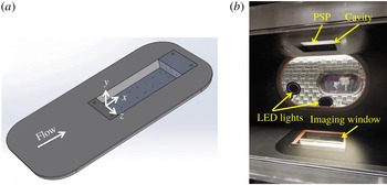
The cavity apparatus is built up from a simple rectangular cutout that is integrated into a tunnel wall insert (figure 1
a). This cavity has a length (
 $L$
), width and depth (
 $D$
) of 203, 102 and 29 mm, respectively, giving an
 $L/D$
ratio of 7. Experiments were performed in Sandia’s Trisonic Wind Tunnel. This is a blowdown-to-atmosphere facility using air as the test gas. The test section is
 $305~\text{mm}\times 305~\text{mm}$
and is enclosed in a pressurized plenum. One porous sidewall and a porous insert on the bottom wall were used to minimize resonance coupling between the tunnel and the radiated acoustic field from the cavity (Wagner et al.
Reference Wagner, Casper, Beresh, Henfling, Spillers and Pruett2015) while also allowing optical access for the PSP.
Experimental set-up: (a) tunnel wall insert containing cavity; (b) PSP set-up.

Run conditions are given in table 1. The Mach number is computed from a centreline static pressure measurement 21.9 cm upstream of the cavity leading edge. The incoming boundary layer to the cavity is fully turbulent. Previous (unpublished) measurements have shown that the boundary layer thickness at the cavity leading edge is approximately
 $0.45D$
. The displacement thickness is approximately
 $0.055D$
while the momentum thickness is near
 $0.05D$
. The walls of the test section remain near room temperature at
 $307\pm 3$
K.
Typical run conditions.

High-frequency PSP from Innovative Scientific Solutions, Inc. (ISSI) was applied to the floor of the cavity. This paint uses a platinum tetrafluorophenylporphyrin (PtTFPP) luminophore that is sprayed on top of a porous ceramic binder. The luminophore is quenched by the presence of oxygen and therefore operates as a pressure sensor. The porosity of the base layer creates additional surface area that allows the paint to respond quickly. Three ISSI LM2XX-DM-400 water-cooled light-emitting diode (LED) arrays were used to excite the PSP over a narrow range near 400 nm (
 $\pm 30$
nm). The lights were all placed in the plenum of the tunnel to locate them as close as possible to the model and to avoid passing light through additional plenum windows (figure 1
b).
The paint emits at wavelengths between 600 and 720 nm. A Photron SA-Z high-speed camera with a 50 mm lens was used to acquire full-view images of the cavity at framing rates of 20 kHz. A 590 nm long-pass filter was used on the camera to remove the 400 nm excitation light and retain the emission from the paint. Imaging was conducted through the bottom window of the test section. Because of its shape, the upstream 7 mm of the cavity could not be seen. Raw images were post-processed using an adaptive Wiener filter in Matlab. This acts as a low-pass filter to reduce additive noise in the images. Images from each movie were ratioed to the mean image from a run. Static calibrations as described in Casper et al. (Reference Casper, Wagner, Beresh, Spillers and Henfling2016a ) were then used to convert the intensity ratios to pressure ratios, yielding the unsteady pressure-fluctuation field.
Kulite XCQ-062-30A (or similar) pressure transducers were used to measure the unsteady cavity pressure fluctuations for comparison to the PSP. The Kulite signal output was passed through an Endevco model 136 DC amplifier, which provides a 10 V excitation and a gain of 100. A Krohn-Hite model 3384 Tunable Active Filter was used to provide a 50 kHz anti-aliasing low-pass Bessel filter. Data were acquired at 200 kHz using a National Instruments PXI-1042 chassis with 14-bit PXI-6133 modules.
3 Experimental results
3.1 Comparison of high-frequency PSP and individual pressure sensors
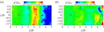
To verify the ability of the PSP to characterize cavity pressure fluctuations, comparisons were made between the PSP measurements and several individual pressure sensors. Figure 2(a) shows a snapshot of a PSP movie with Kulite comparison locations marked with black circles. This case shows predominantly two-dimensional pressure waves travelling within the cavity. These two-dimensional waves appear for a large portion of the dataset, though more complicated pressure fields frequently occur, particularly at the aft end where more turbulent flow is observed (figure 2 b).
PSP measurements on cavity floor, showing the location of comparison pressure sensors marked with black circles: (a) snapshot showing spanwise coherence; (b) snapshot with a more three-dimensional pressure field.

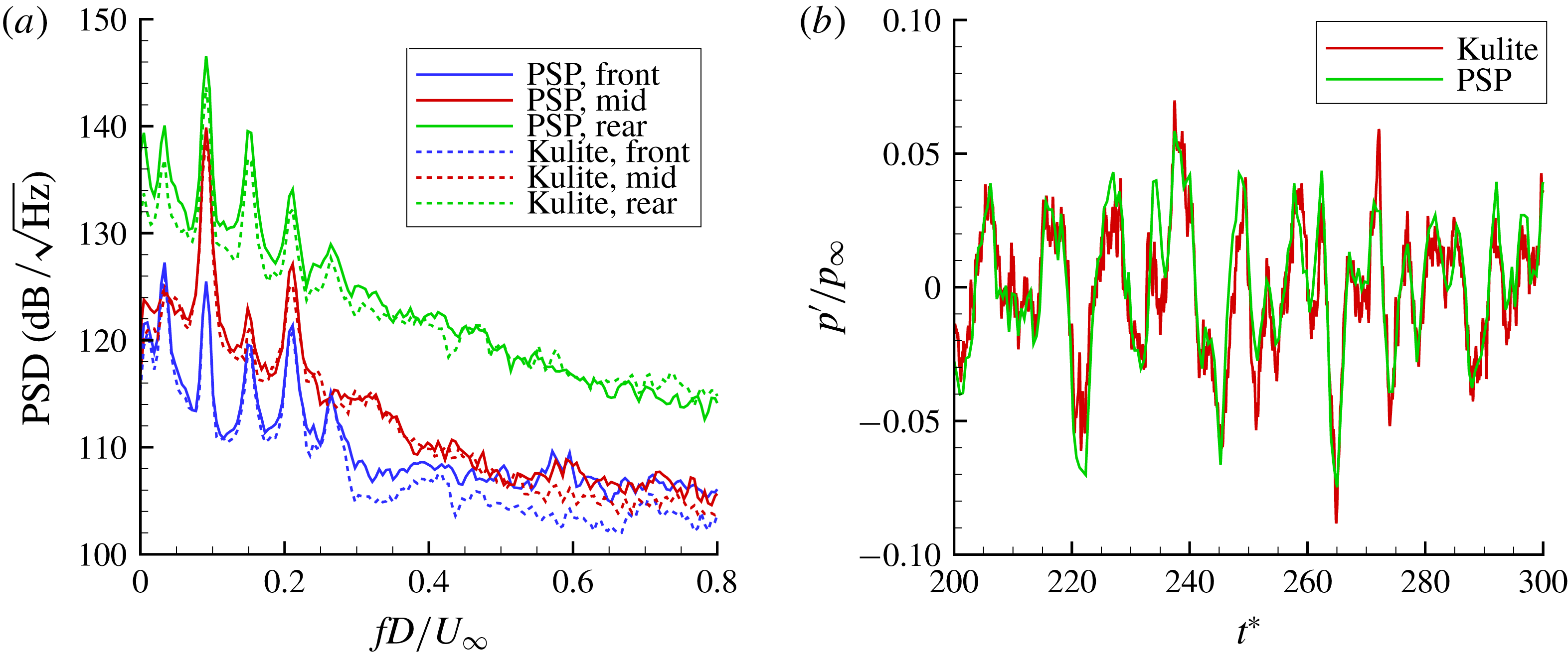
The power spectral density (PSD) of the pressure fluctuations at each Kulite and at a nearby location in the PSP were computed (figure 3
a). The frequency and amplitude of the resonant tones agree between the two methods. In addition to resolving the resonant fluctuations, the signal-to-noise ratio is adequate to resolve broadband fluctuations as low as 106
 $\text{dB}/\sqrt{\text{Hz}}$
. The pressure fluctuations at the cavity front drop below the PSP noise floor above
 $fD/U_{\infty }$
of 0.3 in this case. Figure 3(b) shows comparisons of time traces from a PSP patch and a Kulite pressure sensor near the middle of the cavity. Non-dimensional time was defined as
 $t^{\ast }=tU_{\infty }/D$
. The two measurements track each other well; the instantaneous difference in the two measurements is typically below 1 %, but can increase to 4 % near maxima or minima in the traces. The maximum difference in the overall root-mean-square (r.m.s.) level from the two measurements is 9 %.
Comparison of pressure measurements with Kulite sensors and PSP: (a) power spectral density; (b) pressure trace comparison in the middle of the cavity.

3.2 Spatial distribution of the pressure PSD
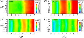
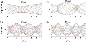
While PSDs are able to show the frequency amplitudes at a given point within the cavity, it is also useful to study the spatial distribution of the PSD amplitudes at each cavity mode frequency. Figure 4 shows these spatial distributions for the first four cavity modes. The spatial distribution of the PSD amplitudes at each mode exhibit a very ordered behaviour that is almost uniform across the span of the cavity. The first-mode activity is highest at the rear of the cavity. Higher modes begin to show additional maxima and minima in the spatial distribution as the mode number increases. The overall amplitude of the fluctuations also increases with downstream distance in the cavity. This behaviour is similar to other PSP observations made on the sidewall (Flaherty et al. Reference Flaherty, Reedy, Elliott, Austin, Schmit and Crafton2014) and floor of a cavity (Roberts et al. Reference Roberts, Stokes, Quinn, Coppin and Birch2016) as well as isolated pressure measurements on the cavity floors (Heller & Bliss Reference Heller and Bliss1975; Murray & Ukeiley Reference Murray and Ukeiley2005). Similar spatial patterns also develop in density and velocity fields (Hankey & Shang Reference Hankey and Shang1980; Kegerise et al. Reference Kegerise, Spina and Cattafesta1999; Garg & Cattafesta Reference Garg and Cattafesta2001; Murray & Ukeiley Reference Murray and Ukeiley2005; Beresh et al. Reference Beresh, Wagner, Casper, DeMauro, Henfling and Spillers2017; Wagner et al. Reference Wagner, Beresh, Casper, DeMauro and Arunajatesan2017).
Spatial distribution of experimental pressure PSD amplitudes at each cavity mode frequency.

The spatial structures of the PSD amplitudes in figure 4 look like standing-wave patterns in the cavity, and indeed much of the literature refers to these distributions in this manner. The standing wave could be generated from upstream- and downstream-travelling waves at the same frequency, but moving at equal velocities in the cavity. However, the upstream- and downstream-propagating waves in the cavity are typically expected to propagate at different velocities (Rossiter Reference Rossiter1964; Heller & Bliss Reference Heller and Bliss1975), which is incompatible with the formation of a standing wave. Instead, an interference pattern will be generated by the summation of upstream- and downstream-travelling waves at the same frequency in the cavity, moving at different velocities. That pattern will be a net downstream-travelling wave whose amplitude is modulated by a fixed envelope as described below.
A simple illustration for this behaviour at each mode frequency
 $\unicode[STIX]{x1D714}_{n}$
was created by adding together a travelling wave of amplitude
 $A_{d}=1$
, moving downstream at
 $0.57U_{\infty }$
, to an upstream-travelling wave with a weaker amplitude of
 $A_{u}=A_{d}/3$
, moving at the speed of sound
 $c$
:
 $$\begin{eqnarray}y=A_{d}\sin (k_{d}x-\unicode[STIX]{x1D714}_{n}t)+\frac{A_{d}}{3}\sin \!\left(k_{u}x+\unicode[STIX]{x1D714}_{n}t-\frac{\unicode[STIX]{x03C0}}{2}\right)\!,\quad k_{d}=\frac{\unicode[STIX]{x1D714}_{n}}{0.57U_{\infty }},\quad k_{u}=\frac{\unicode[STIX]{x1D714}_{n}}{c}.\end{eqnarray}$$
These values are consistent with the Rossiter model of cavity acoustics (Rossiter Reference Rossiter1964). The wavenumber of the upstream- and downstream-travelling disturbances
 $k_{u}$
and
 $k_{d}$
are determined by the mode frequency and convection velocities. Related analyses have been developed by Hankey & Shang (Reference Hankey and Shang1980) and Kegerise et al. (Reference Kegerise, Spina and Cattafesta1999), though this model has been extended here to describe the behaviour and propagation of the unsteady pressure fields, and distinguishes this unsteady behaviour from a standing wave.
The amplitude of the weaker acoustic wave was chosen arbitrarily, but the upstream-propagating wave is expected to be much weaker than the strong shear-layer instability from which it is generated (Alvarez Reference Alvarez2005). This amplitude does not change the conclusions within, only the strength of the interference pattern discussed below. The upstream-propagating wave was given a phase delay of
 $\unicode[STIX]{x1D719}_{u}=-\unicode[STIX]{x03C0}/2$
to locate the minima and maxima in the model close to the experimental observations. This value is again consistent with the Rossiter model where a phase delay of a quarter wavelength fits well with experimental data in many cases (Rossiter Reference Rossiter1964; Heller & Bliss Reference Heller and Bliss1975), though this is not a universal value and other phase delays have been found to agree with other experiments (Kegerise et al.
Reference Kegerise, Spina and Cattafesta1999). Here we use the typical Rossiter values as they were derived from experiments with similar parameters to the current work. The choice of the phase delay only varies the maxima and minima locations in the model, but does not change any other conclusions here.
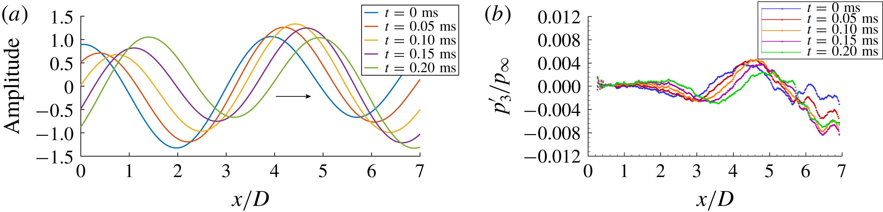
The resulting wave summation is shown at several time steps in figure 5(a). As expected, a standing wave is not generated. A standing wave would have a spatially fixed sinusoidal pattern whose amplitude increases and decreases with time. Instead, the summation is a net downstream-travelling wave whose amplitude is spatially modulated by a fixed cosine function. If several centreline traces from the PSP data are plotted in a similar fashion (figure 5 b), qualitatively similar behaviour between the model and experiment is seen. Both the model and experiment show the modal pressure disturbance propagating downstream while its amplitude is modulated. There is also an overall increase in amplitude of the experimental pressure measurements with downstream distance that is not captured by the model. This increase is a reflection primarily of the growth of shear-layer disturbances as they convect downstream, but the decay of the upstream-propagating disturbances may play a role as well. These phenomena are not included in the present wave interference model.
(a) A few time instants of the simple two-wave summation model for mode 3 showing the resulting travelling wave. (b) A few time instants of the unsteady pressure along the centreline of the cavity, from the experiment.

If many additional different time steps from the model are co-plotted (figure 6
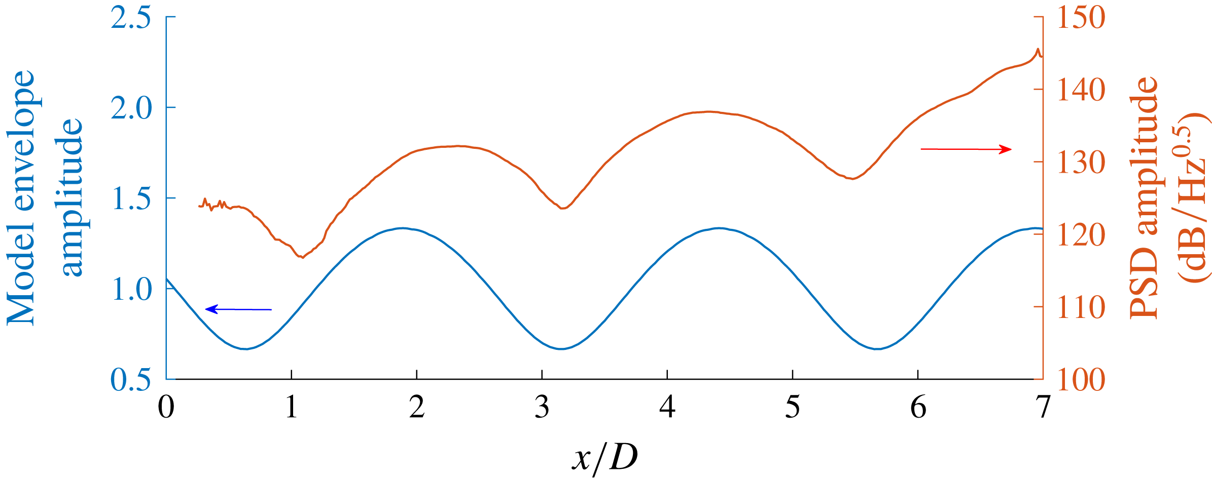
c), the fixed envelope of these travelling waves becomes clear. This envelope has a similar spatial amplitude variation as the experimental spatial PSD results in figure 4(c). Figure 7 shows a direct comparison of the envelope of the mode 3 wave summation from figure 6(c) to the spatial PSD amplitude at
 $z/D=0.51$
from figure 4(c). The envelope behaviour of the travelling waves well represents the spatial distribution of the modal PSD amplitudes, though there are some differences in the wavelength of the distribution at the cavity front. The model assumes constant upstream and downstream convection velocities, whereas, in reality, both the convection velocity and wavelengths vary spatially along the cavity length (Larchevêque et al.
Reference Larchevêque, Sagaut, Lê and Compte2004; Hassan, Labraga & Keirsbulck Reference Hassan, Labraga and Keirsbulck2007). The other cavity mode results shown in figures 4 and 6 show similar agreement between the envelope of the travelling waves and the time-averaged spatial PSD distributions.
Many co-plotted time instants of the simple two-wave summation model showing the resulting travelling wave with a fixed envelope within the cavity.

Comparison of model envelope for mode 3 to the experimental spatial pressure PSD at mode 3 (
 $z/D=0.51$
).

The underlying behaviour of this wave summation is more easily observed by considering the case of equal amplitudes of the upstream- and downstream-propagating waves. The phase delay is also set to zero for simplicity. In this special case, the wave summation can be simplified and rewritten directly as
 $$\begin{eqnarray}y_{2}=2A\sin (k_{ave}x-\unicode[STIX]{x1D714}_{n}t)\cos (\unicode[STIX]{x0394}kx),\quad k_{ave}=\frac{k_{u}+k_{d}}{2},\quad \unicode[STIX]{x0394}k=\frac{k_{d}-k_{u}}{2},\end{eqnarray}$$
which is a travelling wave with wavenumber
 $k_{ave}$
, represented by the sine term, that is modulated by a fixed cosine function (i.e. the envelope that appears in figure 6). In this simplified case, the phase velocity is a constant equal to
 $\unicode[STIX]{x1D714}/k_{ave}$
.
For the case of unequal amplitudes as found in a typical cavity flow (3.1), the qualitative behaviour of the wave summation is the same wherein a travelling wave is modulated by a fixed cosine function. However, the phase velocity will also be spatially varying as discussed in § 3.3. This spatially varying phase velocity can be observed in the unsteady cavity modal pressure fields, as well as in unsteady velocity flow fields in cavity flows (Wagner et al. Reference Wagner, Beresh, Casper, DeMauro and Arunajatesan2017).
The cavity flow is more complicated than this simple model; the downstream shear-layer instability is growing, the upstream acoustic waves are weakly decaying, and there are additional scattering processes and phase delays at the upstream and downstream ends of the cavity that are not accounted for here (Heller & Bliss Reference Heller and Bliss1975; Alvarez Reference Alvarez2005). Despite these limitations, this model gives a straightforward illustration for the observed spatial distribution of the energy found in the time-averaged PSDs of cavity pressure fluctuations, but, more importantly, the model can also describe the behaviour of the instantaneous, unsteady modal pressure field where resonance occurs. This unsteady modal behaviour is described in detail in the following section.
3.3 Unsteady pressure fields
While the spatial distributions of PSDs provide a wealth of information about the resonant properties in the cavity, they are inherently time-invariant. To study the dynamic behaviour, movies were bandpass-filtered around each cavity mode frequency using a wavelet transform. The transform was computed using a Matlab script provided in Torrence & Compo (Reference Torrence and Compo1998) using a Morlet mother wavelet. The wavelet transform coefficients other than those at the mode frequency were set to zero and then the inverse wavelet transform was computed. This effectively bandpass-filtered the pressure data without a time delay and gives analogous results to Fourier space filtering. The filter frequency bandwidth was 200 Hz.
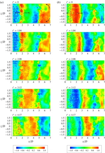
Spatio-temporal cross-correlations of the filtered traces were used to track the average propagation of pressure disturbances on the cavity floor. A point located in the middle of the cavity at
 $z/D=0$
and
 $x/D=3.5$
was used as the reference and then cross-correlated with the other pressure traces in the cavity. Similar results were obtained using other reference points in the cavity. Figure 8 shows the resulting spatial cross-correlation fields for modes 2 and 3. The downstream propagation of structures can be clearly seen. There is also upstream propagation of pressure structures that is particularly evident at the front of the cavity and at the aft wall corners. For mode 2, the coherent structures near
 $x/D=2$
appear to split with time. Part of the structure propagates downstream, while the other half moves upstream. A similar splitting behaviour is observed in anticorrelated structures. For mode 3, a similar behaviour is observed; however, the splitting location moves further upstream to
 $x/D=1.5$
.
Spatial cross-correlations with origin at
 $z/D=0$
and
 $x/D=3.5$
: (a) mode 2; (b) mode 3.

This behaviour is consistent with the superposition of upstream- and downstream-propagating waves. The downstream-propagating structures are observed over the downstream three-quarters of the cavity and probably correspond to the unstable shear-layer disturbances which grow with downstream distance (Alvarez Reference Alvarez2005). The shear-layer disturbances are predicted to spread towards the cavity floor at an angle near
 $45^{\circ }$
(Tam & Block Reference Tam and Block1978), so it makes sense that these waves are only observed beginning some distance downstream of the leading edge.
The upstream-propagating disturbances would be expected to be much weaker than the downstream-propagating shear-layer instability. These disturbances should also decay as they move upstream (Heller & Bliss Reference Heller and Bliss1975; Alvarez Reference Alvarez2005). Since they are weaker, but at the same frequency as the downstream-propagating waves, their effect is to modify the amplitude of the downstream-propagating wave. Therefore, they cannot be independently observed over the aft end of the cavity; only their effect on the downstream-propagating wave amplitudes is seen. Near the leading edge of the cavity, weak upstream propagation is observed at locations not dominated by the large downstream-propagating waves. This causes the apparent splitting behaviour since the upstream waves can only be observed when not dominated by the downstream disturbances.
The velocity of these pressure disturbances was computed by cross-correlating the pressure traces between
 $x$
location pairs within the cavity. A spacing of 30 pixels (approximately
 $x/D=0.5$
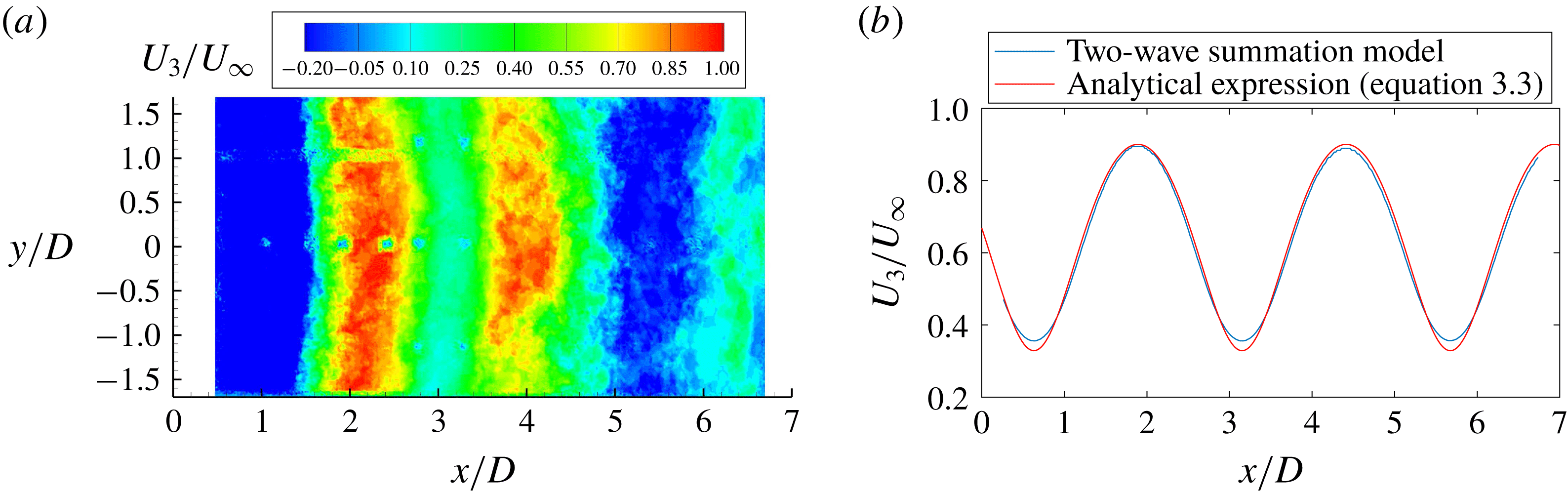
) was used. The maximum cross-correlation corresponds to the time delay for pressure disturbances to move between the two locations. That time delay was then divided by the spacing to estimate the average propagation velocity. Figure 9(a) shows the results for mode 3. The velocity of the pressure disturbances follows a spatial pattern very similar to the spatial PSD in regions dominated by resonance (
 $x/D=1.5{-}5$
). In locations of pressure maxima, the propagation velocity is near
 $0.9U_{\infty }$
. In regions of pressure minima, the propagation velocity drops to
 $0.4U_{\infty }$
. There are also regions of reverse velocity that occur at the cavity front and near the aft wall where more turbulent fluctuations occur. Similar results are obtained at other cavity modes.
Mode 3 phase velocity: (a) from PSP data; (b) from the model.

This velocity can also be compared to the two-wave summation model. In this case, it is important to distinguish group velocity and phase velocity. The group velocity tracks the envelope of
 $y$
. It is typically defined as
 $\text{d}\unicode[STIX]{x1D714}/\text{d}k\approx \unicode[STIX]{x0394}\unicode[STIX]{x1D714}_{n}/\unicode[STIX]{x0394}k$
. Because the upstream- and downstream-propagating disturbances have the same frequency
 $\unicode[STIX]{x1D714}_{n}$
, the group velocity is zero. This means that the envelope of the wave summation is fixed within the cavity, and explains why a fixed interference pattern is observed in the spatial PSDs. This alone does not mean that a standing wave is formed within the cavity. This is an important distinction when interpreting instantaneous modal pressure traces within the cavity which behave as travelling waves, even though, in a time-averaged PSD, the spatial distributions appear as standing-wave patterns. This leads to distinct acoustic properties and a different interpretation of the flow behaviour. The loading distribution generated by a standing or travelling wave will also drive an internal structure in such a cavity flow in a different manner.
The phase velocity of
 $y$
denotes the velocity of the interference pattern, not the velocity of any acoustic signature or turbulent structure (but rather their summation, which results in the net downstream-travelling wave). This is the propagation velocity computed in figure 9(a). It is the velocity of constant phase in the wave summation and is not itself constant because of the unequal amplitudes of the upstream- and downstream-travelling waves. This phase velocity can be analytically derived and substituted with the same amplitudes as in the wave summation model:
 $$\begin{eqnarray}\displaystyle U_{p} & = & \displaystyle \left|\frac{\text{d}x}{\text{d}t}\right|=\left|\frac{\unicode[STIX]{x2202}y/\unicode[STIX]{x2202}t}{\unicode[STIX]{x2202}y/\unicode[STIX]{x2202}x}\right|\nonumber\\ \displaystyle & = & \displaystyle \frac{\unicode[STIX]{x1D714}_{n}A_{d}^{2}+\unicode[STIX]{x1D714}_{n}A_{u}^{2}+A_{d}A_{u}(\unicode[STIX]{x1D714}_{n}+\unicode[STIX]{x1D714}_{n})\cos ((\unicode[STIX]{x1D714}_{n}-\unicode[STIX]{x1D714}_{n})t-(k_{d}-k_{u})x+\unicode[STIX]{x1D719}_{d}-\unicode[STIX]{x1D719}_{u})}{k_{d}A_{d}^{2}+k_{u}A_{u}^{2}+A_{d}A_{u}(k_{d}+k_{u})\cos ((\unicode[STIX]{x1D714}_{n}-\unicode[STIX]{x1D714}_{n})t-(k_{d}-k_{u})x+\unicode[STIX]{x1D719}_{d}-\unicode[STIX]{x1D719}_{u})}\nonumber\\ \displaystyle & = & \displaystyle \frac{{\textstyle \frac{10}{9}}\unicode[STIX]{x1D714}_{n}+{\textstyle \frac{2}{3}}\unicode[STIX]{x1D714}_{n}\cos ((k_{d}-k_{u})x+{\textstyle \frac{1}{2}}\unicode[STIX]{x03C0})}{k_{d}+{\textstyle \frac{1}{9}}k_{u}+{\textstyle \frac{1}{3}}(k_{d}+k_{u})\cos ((k_{d}-k_{u})x+{\textstyle \frac{1}{2}}\unicode[STIX]{x03C0})}.\end{eqnarray}$$
This expression can also be compared to the phase velocity of
 $y$
numerically computed from the wave summation model using a spatial cross-correlation as done with the experimental data. Figure 9(b) shows the result in comparison to (3.3); it is spatially varying and has a magnitude between
 $0.4U_{\infty }$
and
 $0.9U_{\infty }$
.
This sinusoidal result looks very similar to the velocity of the modal pressure field in figure 9(a), but only in regions dominated by the mode resonance (the middle portion of the cavity). In other regions, the model is not fully representative of the experiment. At the cavity front, reverse velocities are observed in the experiment, yet the model predicts a spatially varying positive velocity. As shown before, the downstream-propagating shear-layer disturbances need some distance downstream of the leading edge to propagate to the cavity floor. Therefore, the two-wave summation model cannot represent the experiment at the cavity front. The model also does not capture the reverse velocities at the trailing edge because it does not include the strong turbulent fluctuations found there. The sinusoidal phase velocity also shows up in time-resolved velocity-field data for cavity flows as discussed in Wagner et al. (Reference Wagner, Beresh, Casper, DeMauro and Arunajatesan2017).
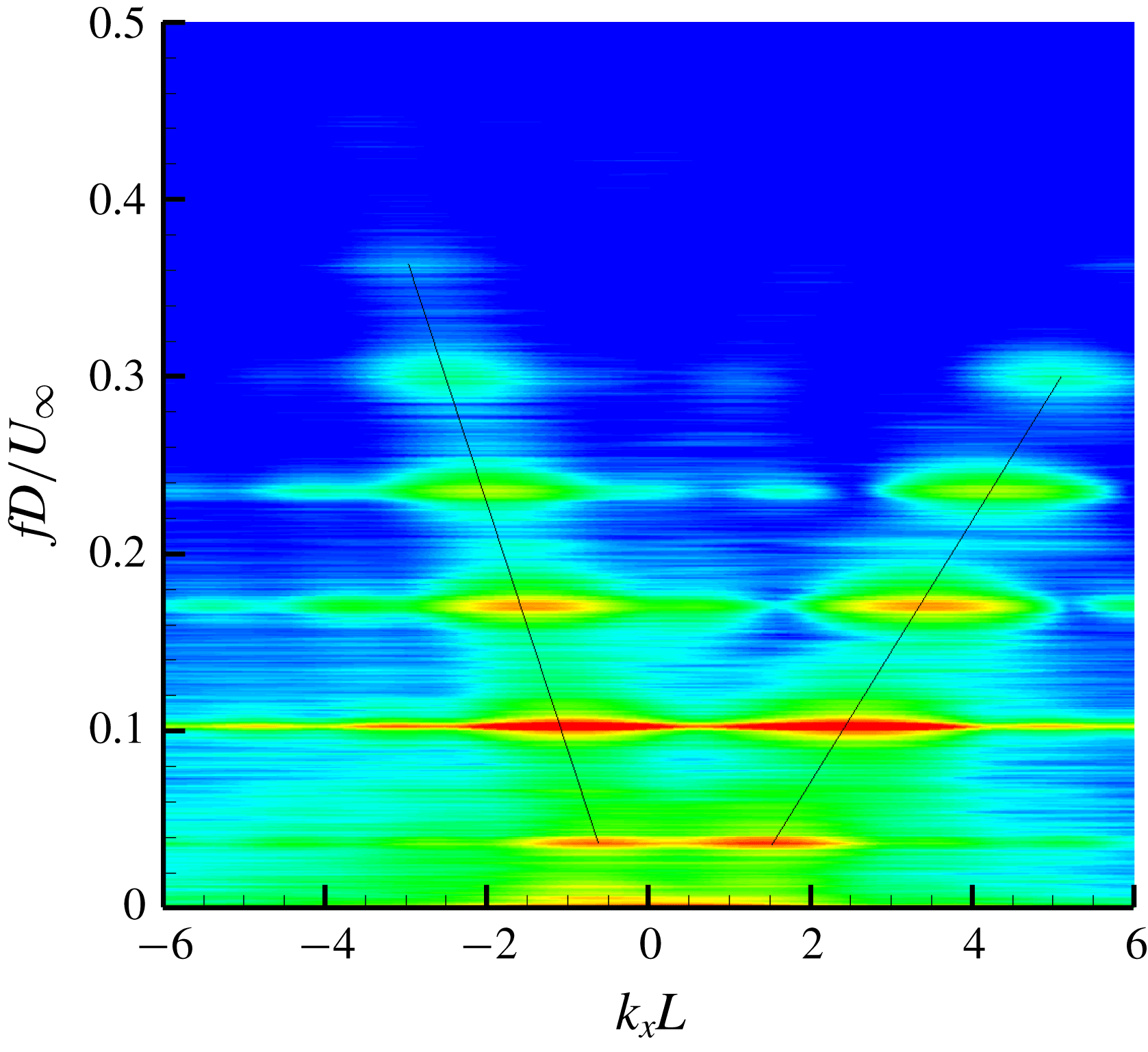
As a final note, the velocity of the upstream- and downstream-propagating disturbances can be independently observed using the wavenumber–frequency spectra as described by Daoud et al. (Reference Daoud, Naguib, Bassioni, Abdelkhalek and Ghoniem2006) and Long (Reference Long2006). This same technique was applied along the centreline of the present data using the fft2 command in Matlab. The resulting wavenumber–frequency spectra are shown in figure 10. Two peaks appear at each cavity mode frequency, one with a positive wavenumber and one with a negative wavenumber. The slope of the line connecting these peaks (when the vertical axis is
 $fL/U_{\infty }$
) gives the convection velocity of the disturbances. Downstream propagation was computed to be an average of
 $0.52U_{\infty }$
, while upstream propagation was 0.9 times the speed of sound computed using
 $T_{\infty }$
. Both are in reasonable agreement with the Rossiter model, though slightly lower than the expected values of
 $0.57U_{\infty }$
and
 $c_{\infty }$
.
Wavenumber–frequency spectra of cavity pressure fluctuations showing both upstream- and downstream-propagating disturbances.

This analysis also hinted at subtle three-dimensional variations in the spatial resonance. Wavenumber–frequency variations near the spanwise edges of the cavity reveal slight differences in the downstream propagation velocities compared to the middle of the cavity. A lower streamwise velocity can be tied to spillage effects at the spanwise edges of the cavity (Beresh et al.
Reference Beresh, Wagner, Henfling, Spillers and Pruett2015). Higher pressure on the outside of the cavity forces flow into the cavity at the spanwise edges, leading to the formation of spillage vortices. DeMauro et al. (Reference DeMauro, Beresh, Wagner, Henfling and Spillers2016) conducted volumetric particle image velocimetry (PIV) measurements for the present cavity, and their measurements were used to estimate the change in the streamwise velocity due to the spillage vortices near the cavity lip line. The streamwise velocity is approximately
 $0.89U_{\infty }$
near the spanwise corner, while it is
 $0.93U_{\infty }$
towards the middle of the cavity. Although this 5 % reduction in the streamwise velocity in the corner of the cavity is small, it will modify the downstream propagation velocity, the wavenumber of the downstream propagating disturbance, and therefore the wavelength of the resulting interference pattern.
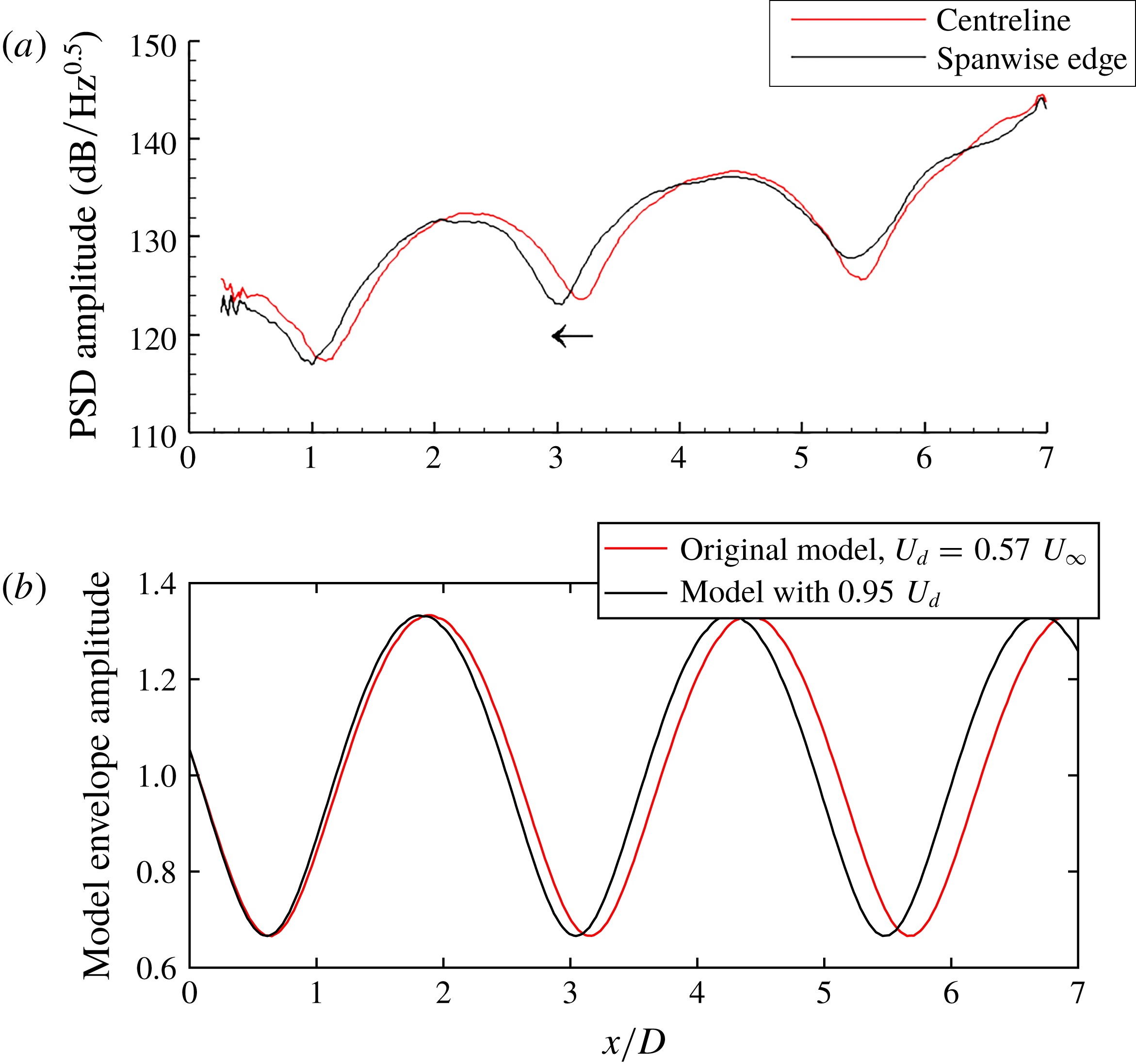
This change in the interference pattern can be seen if the spatial PSDs in figure 4 are revisited. The spatial PSDs for all modes show a subtle ‘bending’ in the upstream direction near the spanwise edges of the cavity. Figure 11(a) shows line plots comparing the mode 3 interference pattern at the spanwise edge of the cavity to measurements further inboard. There is a subtle shift of the interference pattern upstream, primarily over the upstream portion of the cavity. As discussed previously, this is the region of the cavity where resonance dominates the flow field. At the aft end of the cavity, turbulence dominates the measured pressure fluctuations.
Shift in mode 3 spatial distribution at spanwise edges of the cavity: (a) from PSP data; (b) from the model.

The subtle shift in the interference pattern can be tied back to the simple interference model. Figure 11(b) shows a comparison of the original model for mode 3 resonance, in comparison to the results with the downstream propagation velocity reduced by 5 % to match behaviour within the spillage vortices. The model predicts a similar shift in the location of the interference pattern over the upstream portion of the cavity. This correctly matches the experimental results in regions where resonance dominates rather than turbulence. The overall effect of the spanwise variation is minor in the cavity pressure resonance; however, recent measurements with plan-view, time-resolved PIV in similar rectangular cavities (Wagner et al. Reference Wagner, Beresh, Casper, DeMauro, Lynch, Spillers, Henfling and Spitzer2018) show more dramatic changes in modal velocity resonance throughout the cavity.
4 Concluding remarks
High-frequency pressure-sensitive paint (PSP) was used to explore the resonance properties of a
 $L/D=7$
rectangular cavity in Sandia’s Trisonic Wind Tunnel. The paint allowed resolution of the unsteady pressure fluctuations up to 10 kHz. The spatial distribution of PSD amplitudes of the fluctuating pressure field exhibited an ordered pattern, with local maxima and minima along the cavity length. Higher modes had additional maxima and minima. This interference pattern can be explained by the superposition of downstream- and upstream-travelling waves at each mode frequency, moving with different propagation velocities consistent with Rossiter’s model. In a time average, this appears as a standing-wave pattern, though a standing wave is not formed within the cavity when the velocities of the upstream- and downstream-propagating disturbances are different. Instead, this generates a net downstream-travelling wave whose amplitude is modulated by a fixed cosine function. The relative strength of the maxima and minima in the pattern can be related to the relative strength of the upstream and downstream waves. Also, because the frequency of the upstream and downstream waves is the same, the envelope of the travelling wave will be fixed within the cavity and generate the time-averaged amplitude variations observed in the spatial PSDs.
The modal pressure disturbances were tracked along the cavity floor using bandpass-filtered traces and spatial cross-correlations. The predominant direction of the observed pressure disturbances was in the downstream direction. This reflects the fact that the downstream-travelling disturbances are larger than the upstream-propagating disturbances. The propagation velocity of these disturbances showed an oscillatory pattern; higher velocities were observed at maxima in the spatial PSDs, while lower velocities were observed at the locations of minima. This oscillatory behaviour is the phase velocity of the two-wave superposition of the upstream- and downstream-propagating waves. This spatial variation is consistent with the experimental results in areas dominated by cavity resonance. However, at the cavity front where the resonance is weak and at the aft wall where turbulence dominates, the measured propagation velocities differ from the model since the flow is not dominated by the resonance at those locations.
If the velocities of the upstream- and downstream-propagating disturbances are to be individually observed, a wavenumber–frequency spectrum must be used. This showed downstream disturbances moving near
 $0.52U_{\infty }$
and upstream-propagating disturbances moving at
 $0.9c_{\infty }$
, again consistent with the Rossiter model. Small changes in the streamwise velocities at the spanwise edges of the cavity, created by spillage effects, could be tied back to a subtle ‘bending’ of the pressure resonance in the streamwise direction. The spillage locally reduces the velocity of the downstream-propagating disturbance, changing its wavenumber, and therefore the location of the resulting interference pattern that sets up along the spanwise edges of the cavity.
While the new time-resolved data re-emphasizes the usefulness of the Rossiter model in capturing the global behaviour of the cavity flow, the travelling-wave interpretation of the model also helps distinguish time-averaged amplitude variations from instantaneous modal pressure fluctuations. The loading distribution generated by the instantaneous modal behaviour will be different from that predicted by a standing wave, which will generate a different structural response of a store within a resonating cavity flow.
Acknowledgements
S. Arunajatesan, E. DeMauro and M. Barone all provided many insightful conversations on cavity dynamics. T. Grasser and P. Farias provided much needed design and machining support. S. Palluconi of ISSI provided advice on implementing the PSP. Sandia National Laboratories is a multi-mission laboratory managed and operated by National Technology and Engineering Solutions of Sandia, LLC., a wholly owned subsidiary of Honeywell International, Inc., for the U.S. Department of Energy’s National Nuclear Security Administration under contract DE-NA0003525. The views expressed in the article do not necessarily represent the views of the U.S. Department of Energy or the United States Government.