One of the defining characteristics of the industrial revolution and its aftermath was the increasing opportunities for travel. Although better roads and better carriage design had increased attainable speeds before the transport revolution, they remained restricted by the physical limitations of the horses that powered them. On water, sailors remained at the mercy of the wind.1
Bagwell, Transport Revolution.
Ville, “Transport”; and Weyl, Passenger Traffic, p. 110.
Improvements in passenger transport technology can have many effects: raising or lowering costs, speeding it up or slowing it down, making it more or less comfortable, and leading to more or fewer deaths and injuries. The correct way to analyze transport improvements, ex ante and ex post, is via cost-benefit analysis. In recent years governments and others have improved the quality of such analyses; in this article we apply those insights historically.3
See, for example, the websites of the Department for Transport's Transport Analysis Guidance, available at www.webtag.org.uk; and Leeds University's Institute for Transport Studies, www.its.leeds.ac.uk.
Great Britain, Transport, pp. 196–97.
Economic theory states that an individual's valuation of time is the opportunity cost, that is the value of the alternative use for that time. For those traveling on work time, the value of an hour saved is the hourly employment cost, because if travel were instantaneous, an hour of travel could be replaced by an hour's productive work.5
Costs include gross wages, payroll taxes, and employer pension contributions, as well as a share of overhead costs (office space, back office functions, and so on), which add 21.2 percent today. Where an individual's wages are unknown, the usual proxy is the average wage for users of that transport mode. Department for Transport, “Values,” p. 2, paragraph 1.2.4 and p. 4, table 1.
The U.K. government currently values leisure and commuting time at 46 percent of average take-home wages. This is for working age people and pensioners, with the latter's valuation 25 percent lower than the former's. In order to correct for the lower ratio of pensioners to working age people in the nineteenth century, we increase the overall figure by 4 percentage points, to 50 percent of the take-home wage. Ibid., paragraph 1.2.17.
That time savings are not included in GDP is not of concern to economists and economic historians. Our interest is in consumer welfare gains from new technology, whatever form those gains take. If they are valued by consumers then they are part of consumer surplus, if they are part of consumer surplus then they should be included in cost-benefit analysis.7
Great Britain, Transport, 3.10–3.12, pp. 57–58.
The form of cost-benefit analysis used by historians to study railways is known as “social savings.” This approach was first used in the 1960s in the pioneering works of Robert Fogel and Albert Fishlow.8
Fogel, Railroads; and Fishlow, American Railroads.
Foreman-Peck, New Perspectives.
The social saving methodology, as used by Fogel, Fishlow, and Gary Hawke in their original studies measures the cost to society of doing exactly what it did with the railways, without them. Elementary economics tells us that quantity demanded rises as price falls, and thus, because prices were lower in the railway era, the social saving will overstate the benefit of railways to society: some people would not have been willing to pay the higher price to travel. The extent to which travel increases depends on the (generalized) price elasticity of demand, which is (implicitly) assumed to be zero in the social saving methodology. Fogel sets out the formula to convert the social saving into the increase in consumer surplus, according to different estimates of the elasticity of demand.10
Fogel, “Notes,” pp. 10–11, equations 11 and 12:


Where St is the true social saving, and S0 the zero elasticity social saving already calculated, ε the elasticity, and ϕ the ratio of prices without railways to with railways. The intuition is that the higher the price ratio, the more journeys will not now take place.
HISTORIOGRAPHY
Hawke calculated the social savings from goods and passenger travel for English and Welsh railways from 1840 to 1870, with particular emphasis on 1865. Hawke's passenger methodology is simple and correct. He finds the distance people traveled in each class and assesses the means by which they would otherwise have traveled. He then finds the total cost by each method, with the difference representing the social saving. This is calculated as either 2.1 percent or 5.8 percent of GDP, depending on whether first-class rail is held to be as comfortable as the inside of a stage coach, or traveling by private carriage, generally known as a post-chaise.11
Hawke, Railways, pp. 48–49, table II.02. The figure of 2.1 percent is incorrect; it should be 1.6 percent as given on p. 44.
These findings have not gone unchallenged. In his review William Baker notes that Hawke's social saving estimate is roughly double those of Fogel and Fishlow, with much of the difference coming from “Hawke's attempt to quantify the greater convenience and comfort of rail over non-rail passenger service.”12
Baker, “Railways,” pp. 718–19.
Ibid., p. 719.
Fishlow, “Railways,” pp. 75–76.
Gourvish, Railways, pp. 58–59, expressed here as a percentage of U.K. GDP for ease of comparison.
Hawke does not include any benefit for time savings, arguing that inflexibility of working hours meant that few workers were able to use the additional time saved to work, so it is likely that it was primarily leisure, not production that increased. That said, he acknowledges that excluding time savings imparts a downward bias, in that some travel was for business purposes, and clearly faster journey times did allow greater production. He argues that this bias is likely to have been small, given that the majority of miles traveled were third class. He also argues that because workers did not have a choice as to working hours, the theoretical construct that workers value leisure at the wage rate is invalid, and therefore he regards such time saved as worthless. Finally, he notes that if we are to compare leisure time savings with GNP, we would need to include the valuation of all leisure time in our estimate of GNP.
Hayden Boyd and Gary Walton, who estimate the social saving from faster passenger rail travel in the United States in 1890, argue that it is legitimate to compare the value of time saved with money GNP providing that we interpret the social saving result carefully. They note that because much of the social saving from faster passenger travel comes from increased leisure time, the social saving “measure does not show how much GNP would have been reduced if the railroad had not been available to travellers. It does show in the aggregate the percentage of GNP travellers in 1890 would have been willing to exchange for the opportunity of travelling by rail rather than by the next best alternative.”16
Boyd and Walton, “Social Savings,” p. 240.
A good discussion can be found in Harrison and Quarmby, “Value.”
Boyd and Walton note that, contrary to Fishlow's assumption, it was cheaper to travel by canal and steam boat than by railway, and yet people overwhelmingly chose to travel by train. They note that an analysis including only fares would generate the clearly incorrect result that passenger rail travel created negative social savings. That people chose to use the more expensive railway rather than the cheaper boat must mean that people were prepared to pay to save time, and therefore that economic historians should include that valuation in their estimate of social savings.
This article revises and extends Hawke's social savings for passenger rail travel in England and Wales. It seeks to achieve five things. First, to use modern economics to value the time saved. Second, to improve the quality of Hawke's analysis of the monetary savings available from railways for 1865. Third, to extend the time and money social savings estimates to cover the period 1843 to 1912. Fourth, to divide social savings into money and time components, and between premium and third-class passengers. Finally, to express the social savings from passenger rail transport as a proportion of economy-wide total factor productivity growth. This article generates a better understanding of this new technology's nature, the sources of its welfare gains and the distribution of those gains. As the period progressed, time savings became relatively more important relative to fare savings. This was not so much because trains became quicker—although they did—but rather because over time an increasing number of passengers were drawn from poorer sections of society, whose only other realistic method of travel was to walk. By 1912 passenger railways' social saving was 14 percent of GDP, of which 10 percent came from time saved, and 4 percent from reductions in fares.
ANALYSIS OF SOCIAL SAVINGS IN 1865
A social savings calculation requires an alternative, counterfactual, mode of transport. Hawke uses two different counterfactuals, one based on Lardner's book—first-class rail equivalent to inside a stage coach, other classes to seats outside the coach—and another based on the 1867 Royal Commission report—equating first-class rail with traveling post chaise, second-class with inside the stage coach, and third-class with outside it. Hawke uses Lardner's comparison for years up to 1850, and that of the Royal Commission for years from 1865, with a linear transition from one “comfort comparison” to the other, reflecting the steady relative improvement in railway comfort. Philip Bagwell shows that posting passenger miles were almost as high as coaching miles prior to the railway age, and that the number of post horses went down rapidly after the introduction of railway services. It seems most plausible, therefore, that first-class rail travel replaced posting as soon as the railway began. We therefore prefer the Royal Commission approach to that of Lardner, and use it throughout this article.18
Hawke argues that the nature of rail journeys meant that the only alternative was coaching, with sea transport essentially irrelevant. In any case, steam ships depended on essentially the same technology as railways, so a counterfactual of steam ships but not railways has little intuitive appeal.
We argue, however, that third-class passengers would not, in the absence of the railways, have traveled by coach, but would instead have walked. Although both Lardner and the Royal Commission base their third-class comparisons on outside coach fares, there is ample evidence that the sort of people who traveled third class would never have been coach travelers, evidence noted by Eddie Hunt and acknowledged by Hawke.19
Hawke, “Railway Passenger Traffic”; and Hunt, “Review.”
Parliamentary Papers: Report from Commissioners: Railways, 1867, vol. 38, part 1, p. liii, paragraph 118.
Parliamentary Papers: Report from Commissioners: Railways, 1867, vol. 38, part 1, p. cvii, paragraph 2.
Parliamentary Papers 1840, vol. 13, p. 285 (479), paragraph 4,862.
Parliamentary Papers 1840, vol. 13, pp. 242–43 (436–37), paragraphs 4,249–4,265.
Miles Traveled
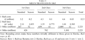
The first step in estimating social savings is to assess the number of passenger miles traveled in each class in 1865. Hawke takes the total railway receipts and average fares by class in England and Wales from the Railway Returns. These data are as authoritative as any nineteenth-century data. Dividing receipts by the fare per mile gives the number of miles traveled. There are, as Hawke notes, “some complications.”24
Hawke, Railways, p. 40.
Parliamentary Papers 1876, vol. 65, p. 98 (p. 226).
Hawke assumed that all season ticket holders paid a third-class fare and so treats them as third-class passengers for his analysis.

TIME SAVINGS
We noted earlier that the modern transport literature views the cost of transport as a generalized cost, made up of money and nonmoney components. Although this method of expression is relatively new, the concept is not. Lardner, for example, included the time saving in his analysis of the importance of railways, and the Select Committee of 1854 and Royal Commission of 1903–1904 were also aware of the issue.27
Lardner, Railway Economy, p. 164; Parliamentary Papers 1854–1855, vol. 10 quarto, pp. 1220–21; and Parliamentary Papers 1906, vol. 46, pp. 675–77.
In the nineteenth century trains were much faster and often much more frequent than coaches, and became both faster and more frequent over time. Furthermore, train companies believed that customers valued speed: it played an important part of their advertising strategy, and they were keen to set new records. In addition, faster trains were generally more costly to operate, so given increasing speeds, we know that railway companies believed that passengers were prepared to pay more for faster travel. This would also fit with the finding that Britain had faster trains than elsewhere in Europe: as the richest country, British people were rationally prepared to pay more to save a given amount of time, and train companies catered for their needs accordingly.28
Foxwell and Farrer, Express Trains, pp. 66, 163–79.
There were two contemporaneous estimates of the value of faster travel in Victorian Britain. Lardner argued that in 1848 coaches traveled at 7.5 mph and trains at 25 mph. With 170 million passenger miles the time saved amounted to just under 16 million hours, which at Lardner's value of time of 6d per hour implies a saving of £0.4 million.29
Lardner, Railway Economy, p. 164.
Quoted in Simmons, Victorian Railway, p. 373.
He assumes coach and rail speeds of 10 and 30 mph respectively, but only attributes value to the time of 20 percent of passengers, that is, 445.69m passenger miles, with time valued at 8d per hour. Gourvish, Railways, p. 59. Foreman-Peck, New Perspectives.
In order to value the time saved, we first calculate average travel speeds by rail and prerail methods, from which we calculate the number of hours saved. We do this using both the actual journey time itself, and including an allowance for the lag when the train (or coach) does not depart at the traveler's preferred time. We then assess the value of one hour of time saved, and use that to calculate the value of total time saved.
Train Speeds
Although we know that trains were faster than coaches, and that train speeds increased over time, there has been no systematic study of average train speeds. That is not to say that we know nothing—Ernest Foxwell and Thomas Farrer, for example, give good data on the number and speed of express trains between 1871 and 1888—but nevertheless our knowledge is surprisingly weak given the extent of the railway literature.32
Foxwell and Farrer, Express Trains, pp. 66–69. Thus, for example, Bagwell's generally authoritative book makes no mention of railway speeds prior to 1914 (Bagwell, Transport Revolution), Ville simply writes of “substantial improvements in speeds.” Ville, “Transport,” p. 307; whereas Thomas notes only that “Locomotives roared through the countryside at speeds of up to 40 miles per hour,” Thomas, “Service Sector,” p. 102.
Of course, neither trains nor coaches would always have operated precisely to their time-tables, but it seems more likely that punctuality was better on the railways than on coaches, and that punctuality improved over time. Thus although timetables will overstate the true speeds, the effect is likely to be small and declining over time. Bradshaw, “Bradshaw's”; and Bates, Directory.
Sample size was determined to generate stable results. Thus, for example, the additional of journeys 45–50 did not alter our speed estimates; similarly, restricting our minor journeys sample to looking only at places with a population of over 15,000 does not alter our estimates. This gives us confidence that our sample generates accurate results.
The important routes are defined by the likely traffic on them.35
We ranked journeys by the product of the population of the two places, divided by the distance. This captures two intuitions: that more journeys will be made when there are more people in the two places (the benefit of travel increases), but that there are likely to be fewer journeys if the distance is long (the cost of travel increases). In effect this model assumes that people travel to meet other people, rather than to visit a scenic place, such as the seaside, and has the characteristics of a gravity equation.
A full list is given in the Appendix.
For tractability we limit ourselves to weekday trains.
Rather than using a simple average for each route, we follow best practice and use a “twin-peak” weighted average, that is, we assume more people wish to travel at peak times than at off-peak times, and give higher weight to trains at those times in calculating the average speeds on each route in each benchmark year. We experimented with many different weightings, including uniform demand over the 24 hour period. Contrary to expectations, the pattern of demand does not alter the results by more than a few minutes, and does not alter the final social savings results. Both coaches and trains were sufficiently frequent, and uniform enough in speed, that the precise allocation of passengers to individual trains is of no great importance. Route speeds are averaged in proportion to the route's importance, as defined by the likely traffic on the route. We assume any passenger could have traveled on any train. In reality this was not the case in the early years, when not all trains had third-class carriages. This bias is small, because only a small proportion of passengers traveled in third class in the early years.
Thus, for example, the Great Western Railway shortened routes from London to South Wales and the West by building new cuttings through hills it previous detoured around. As such, it lost its nickname of the “Great Way Round.” Cain, “Railways,” p. 93.
Speeds on important routes were higher than on more minor routes. To find the speeds on minor routes we took a simple average of the speed of the first train after 7AM into each of the 222 towns with a population over 12,500 in 1901, in each of our four railway benchmark years.40
Journeys over two hours were excluded, and the remainder varied from the very short (Glossop to Dinting, 1 km) to the rather long (Peterborough to Doncaster 120 km), the average was 28 km. The towns are listed in the Appendix.
We give important journeys a weighting of 52 percent. This is based on working out the implicit demand for travel between each of the 185 towns and each of the other 36,000 settlements in Britain listed in the Ordnance Survey Gazetteer, according to the earlier formula that implicit demand equals the product of populations divided by the distance, with a minimum distance of 5 km. Of total implicit demand, we assume that the average speed for important journeys holds only for those journeys themselves, with other journeys over 120 km being proxied by the simple average of important and minor journeys speeds, and all other journeys under 120 km by the minor journey speed. It is possible to argue for different weights, but given the numbers it is hard to see the overall average presented here being wrong by more than two or three miles per hour at most.
Bates, Directory, important routes.
http://www.ramblers.org.uk/info/practical/navigation.html#Planning. The recommendation is three to four km per hour, we use four km. Summerhill uses three km per hour, but it seems likely that walking speeds were higher in England and Wales owing to better quality roads and higher nutritional standards. Summerhill, “Big Social Savings,” p. 85.

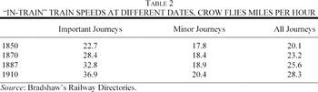
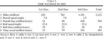
Table 2 shows that train speeds on important routes were considerably higher than on minor ones, and grew more quickly over time. Minor journeys generally stopped at more stations en route, which limited the potential for cutting journey times. Overall, a rise in speeds from 7.8 and 2.5 mph in the prerailway era to 20 and then later to 28 mph in the railway era represents a major improvement in quality for consumers. Table 3 sets out the number of hours saved.

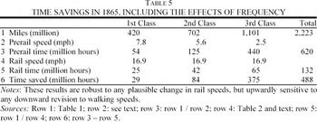
Railways were much faster than the alternatives. The time needed to travel fell by over eighty percent, to 99 million hours. It is worth emphasizing that this figure is robust. Were trains to have been 10 percent slower, the overall time saved would fall by under 2.5 percent. In contrast, were William Summerhill's assumption that walkers would have averaged 2 miles per hour, rather than 2.5, to be accurate, the number of hours saved would increase by more than 20 percent, to 595 million hours. As we have noted, our assumption of 2.5 miles per hour is the highest plausible average and as such the number of hours saved is almost certainly too low rather than too high. The vast majority—over three-quarters—of time saved was saved by third-class travelers, both because they represented the largest single category of traveler, and because their alternative methods of transport—walking, or wagons moving at walking pace—were very slow. As with all social savings numbers, we need to be careful as to how these figures are used. Just as Hawke's social saving figure of £48 million did not mean that society spent £48 million less on transport in 1865 than at some previous date, neither does Table 3 mean that 485 million hours were actually saved. Rather, it tells us that to make the journeys made by rail, without the railways, would have taken an additional 485 million hours.
Service Frequency
We know that trains were more frequent than coaches, and that people value frequency, because it reduces the overall journey time. Contemporaries appreciated this. Thus Mr. Edward Bury, superintendent of locomotive power on the London and Birmingham Railway, told the 1840 Committee on Railways that “The great advantage to the public will be, in not having a single train per day carrying all the passengers that go, but in having a multiplicity of trains throughout the day,” adding later in his evidence that “I think the public would not have the convenience the railway ought to give them, unless there were frequent trains.”44
Parliamentary Papers 1840, vol. 13 p. 112 (306), paragraph 2,327, p. 115, (309), paragraph 2,392.
Bates, Directory, pp. 30, 32, 34–36.
We model the effects of changing frequencies. For very frequent services (say, six per hour or more), the evidence is that people turn up randomly, and catch the next available service. In this case average waiting time (half the service interval) can simply be added to the journey time. When frequencies decrease, people cease to arrive at the station randomly. Although this means that average waiting times at the station do not increase much as frequencies decline, passengers do incur disutility because the train does not go at the time that they would like it to, forcing them to remain in one place when they would by definition rather be in another. They can use the time in the original place, but it is worth less to them than that time would be at their destination. The transport economics literature converts the nominal waiting time (the time between preferred and the actual departure time), into what is termed “in-vehicle time” (IVT) equivalent minutes. This is the additional in-vehicle time assessed as having equal disutility to the delay in leaving. Waits of up to ten minutes are simply added onto the journey time, but (nominal) waits of over ten minutes are valued less highly, because the person can do something in their place of departure.
Mark Wardman reports that current U.K. practice is to convert nominal waiting times into in-vehicle equivalent times by multiplying the former by one for times up to ten minutes, and by 0.8, 0.55, and 0.43 for half-hourly, hourly and two-hourly services.46
Wardman, “Public Transport,” paragraph 2.5.
We regress these conversion factor onto time and log time, to get the result that the conversion factor equals 1.58 + 0.0002time – 0.57logtime. This predicts values of 0.99, 0.75, 0.58, 0.43 and 0.1 for gaps of 11, 30, 60, 120 and 1,440 minutes, very close to the values given by Wardman.
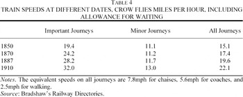
There were almost four times as many useful services on important routes in 1910 as in 1836 or 1850, but there were still sufficient coach and train services in the earlier years that increasing frequencies did not radically alter the pattern of overall improvement given by the in-vehicle speeds themselves. The same is true for trains on minor journeys. As we noted earlier, we recorded details of the first train to arrive after 7AM in each town, and so the wait after 7AM can reasonably be taken as a measure of the nominal waiting time. This falls from 74 to 53 minutes between 1850 and 1910, or 34 to 30 IVT equivalent minutes—a trivial improvement. The hardest calculation to make is the fall in waiting times from coaches to the initial trains, because we have virtually no information about coaches on minor journeys. That said, the issue is second order, as only second-class passengers are assumed to travel by coach. If we assume one coach per day on minor routes the average nominal wait would be 12 hours, equivalent to 82 IVT minutes, which reduces the average speed from 7.8 mph to 5.6 mph. In contrast we assume that both private coaches and walkers did not have to wait at all: both could set out at a time of their choosing. The full results are given in Table 4, and comparing Tables 2 and 4 shows that including frequency does not alter the pattern of change over time in any meaningful way.

Again, combining our data for miles traveled with the speed data in Table 4 allows us to calculate the number of hours saved, including an allowance for waiting (see Table 5). Including frequency in the analysis proves to have little effect, with an overall time saving different by under 1 percent. This is caused by two factors. First, the delay to second-class passengers in waiting for the relatively infrequent stage coach was sufficient to offset the delays for first- and third-class passengers waiting for the train. Second, Britain was already a remarkably developed economy prior to the railway. Stage coach services were particularly extensive on core routes, but were also well established on relatively minor cross country journeys. Bates records regular, usually daily, services on 786 different routes excluding those that started or ended in London.48
Bates, Directory, pp. 85–138.
Bogart, “Tunpike Trusts.”
Crafts and Mulatu, “Location.”

The Value of Time Saved
As we noted earlier, the value of time saved during working hours is taken as the gross wage rate.51
In modern studies it is necessary to include overhead costs, but there were no payroll taxes and few employer-funded benefits in the nineteenth century, so overhead costs would have been small enough for us to disregard them without any significant loss of precision.
Edwin Chadwick, Parliamentary Papers: Report from Commissioners: Railways, 1867, vol. 38, part 1, p. 838, paragraph 17,181.
Average earnings for both sexes. Feinstein, “New Estimates,” p. 604. In that this figure is for the United Kingdom, it understates wages in England and Wales, although the margin of error will be small. 1882–1912 using Feinstein, “Changes,” appendix 24, p. 264; and 1843 to 1882 using Feinstein, “Pessimism Perpetuated,” p. 653.
This is the average salary of those in Census class V, Merchants etc., using information from Routh, and assuming that commercial travelers earned £99 a year, Routh, Occupation 1906–79, p. 63.
The next issue is the proportion of people traveling during work time, and the proportion of commuting and leisure travel. As we noted earlier, those traveling on business should have their time proxied by wage costs, whereas those who were traveling in their own time should have their time valued at half their take-home wages if the time saved would otherwise have been spent in a train or carriage, and at their wage rate if the time saved would otherwise have been spent walking. We simply do not know what proportion of travelers in any class were traveling on business in 1865. The sensible way to proceed is to assume first that all travel was on business, and second that no travel was on business, and then to consider the plausible bounds within these extreme cases.
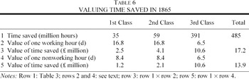
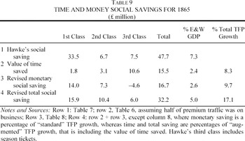
Table 6 gives a range of figures from £14 million to £17 million depending on the proportion of premium class passenger traveling on business. It seems implausible to believe that—say—less than one-quarter or more than three-quarters were traveling in work time. As such, the plausible bounds are £14.7 million—£16.3 million. Our central estimate—£15.5 million—simply assumes that half of those in premium classes were on business. It is possible to argue for other proportions traveling on business, but it would seem hard to imagine that this estimate is out by more than £1 million. Similarly, because we have good evidence for the average wage of those traveling by third class, it is only the wage that we assign to the premium-class passengers that is a source of possible error. Again, the size of any error is limited: were we to raise or lower that wage by as much as a third, the estimate of the value of time saved would change by only 10 percent. £15.5 million is a significant sum, and represents over 2 percent of GDP. Time savings clearly mattered.

MONETARY COSTS
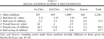
Table 7 sets out Hawke's estimates of the monetary savings that came from the railway's invention. He assesses the alternative cost of travel in 1865 at £60m, which gives a social saving of £48 million, or 5.8 percent of GDP.

Revisions to Hawke's Money Social Savings
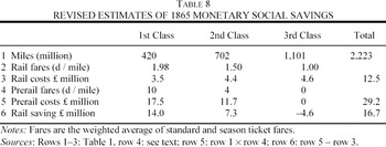
We make three revisions to the calculation of monetary social savings for 1865. First, we noted earlier that data from the Railway Returns allows us to allocate season ticket holders more accurately across classes.55
Parliamentary Papers 1876, vol. 65, p. 98 (p. 226).
Hawke reports coaching costs as 4d inside, and 2.5d outside, similar to figures given elsewhere.56
Copeland, Roads, p. 93. As Gourvish has noted, Hawke mistakenly used the cost of inside, rather than outside, the coach for second-class rail travel in his table II.02 Lardner counterfactual, which overstates the social saving by a quarter. The number given in the text on page 44 is correct. Gourvish, Railways, p. 34; and Hawke, Railways, p. 44, table II.02.
Fishlow, “Railways,” p. 76.
Parliamentary Papers: Report from Commissioners: Railways, 1867, vol. 38, part 1, p. liii, paragraph 118. Charging per coach rather than per person is to be expected because the costs were essentially invariant in the number of passengers. This is generally clear from the context, but is made explicit in a 1761 advert in The Ipswich Journal, the 1802 accounts of a Suffolk postmaster, a 1793 article in The Leicester Journal, and the 1823 Best family account books, all quoted in Copeland, Roads, pp. 155–59. In addition, articles in The Times always refer to the cost of hiring a chaise and pair per mile, with no suggestion that this is per person per mile. See references in note 28
Mr. Henry Gray, Chairman of the Association of the Postmasters, when interviewed on post horse duty, stated in answer to the question “How have you calculated how many passengers on an average you carry post, for each horse hired?—Two I should say, four is considered the average with a pair horse carriage,” Parliamentary Papers 1837, vol. 20, p. 9 (305), paragraph 145.
References to 1s: Issue 5400, 26 April 1802, p. 3, column C; issue 11570, 29 May, 1822, p. 3, column A, issue 11598, 01 July 1822, p. 3, column F, and issue 11822, 18 March 1823, p. 3, column D. References to 1s 3d: Issue 5198, 29 August 1801, p. 3, column A; issue 5202, 3 September 1801, p. 2, column C; issue 8343, 17 October 1814, p. 2, column D; issue 9450, 21 February 1815, p. 3, column G; issue 11152, 24 January 1821, p. 4, column A; issue 11217, 11 April 1821, p. 3, column A; issue 11822, 18 March 1823, p. 3, column D, and issue 11873, 16 May 1823, p. 4, column D. References to 1s 6d: Issue 7246, 1 January 1808, p. 3, column, B and issue 9008, 6 September 1813, p. 3, column E.
Parliamentary Papers 1837, vol. 20, p. 9 (305), paragraph 145, p. 11 (307), paragraph 178.
Copeland, Roads, p. 155, see also similar figures on pp. 156–60.
369 million miles divided between 25,053,443 passengers, both from Railway Returns, Parliamentary Papers 1866, vol. 63, p. 36.
Mr. Henry Gray, Chairman of the Association of the Postmasters, stated that four would be average, but because this is the maximum, it is hard to believe that this was also the average. Parliamentary Papers 1837, vol. 20, p. 9 (305), paragraph 145.
Notwithstanding the ceteris paribus rise in the estimate of social savings from the better assignment of season ticket revenues, the figures given in Table 8 are much lower than those presented by Hawke. The skepticism of Baker and Fishlow proves to be well-founded.65
The 10d figure can also be applied to other estimates. Thus, for example, Gourvish's upper-bound social saving falls from £128.2m to £62.1m, and from 22.9 percent to 12.6 percent of England and Wales GDP. Gourvish, Railways, p. 59.

As we now have a revised figure for the monetary saving, and a figure for the value of time saved, we can calculate the total social saving. Hawke divides the social saving for railways in England and Wales by GDP for the United Kingdom. As Gourvish noted, this is inappropriate.66
Ibid., p. 36.
Crafts, “Regional GDP.”
Table 9 tells us that both the time and money savings were significant, and of approximately equal magnitude. Together they amount to 5 percent of England and Wales GDP, one-third lower than Hawke's estimate. For premium passengers the gains were primarily monetary: lower fares represent around 90 percent and 70 percent of the total gains to first- and second-class passengers respectively. For third-class passengers the picture is very different: their fares increased by £4.6 million, but they saved £10.6 million worth of time.

We noted earlier that social savings are equivalent to (cumulative) TFP growth. It is thus straightforward to express the social savings results given here as a percentage of economy wide TFP growth in this era. Monetary social savings of 2.6 percent by 1865 equate to an annual rate of 0.07 percent between the opening of the Liverpool and Manchester Railway in 1830 and 1865. This accounts for 9.7 percent of economy-wide TFP growth of 0.75 percent in this era.68
Crafts, “Steam,” table 1. The figure is for 1831–1871, we assume that it holds for 1831–1865.
That railways were a “high technology” good can also be demonstrated by looking at the rate of price falls (TFP growth) compared with those elsewhere in the economy. Table 9 shows that the monetary and time costs of a representative 1,000 passenger miles of travel in 1865 were £5 6s 7d and £2 1s 7d respectively. Using prerailway (1830) travel technology these costs would have been £12 10s 4d and £9 9s 2d, falls of 2.5 percent and 4.4 percent per annum respectively. These are considerably higher than U.K.-wide TFP growth, confirming the status of railways as a high technology product.
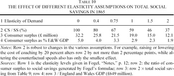
We noted earlier that the social savings methodology overstates the gain in consumer surplus, because it implicitly assumes zero price elasticity of demand. Table 10 sets out the ratio of consumer surplus to social savings at different elasticities.

By definition, the different elasticity assumptions give significantly different results, from 1.9 percent of GDP to 5 percent of GDP. In their analysis of U.S. passenger railways Boyd and Walton assume unitary price elasticity, an assumption endorsed by Fogel, and used by others, including most recently Summerhill.69
Boyd and Walton and Fogel also give figures for other elasticities, from zero to two, Summerhill also notes other studies that have used unitary elasticity. Boyd and Walton, “Social Savings,” p. 249, table 3; Fogel, “Notes,” p. 11; and Summerhill, “Big Social Savings,” p. 82.
The “famous rule of a half” is a linear approximation to this. Great Britain, Transport, p. 65, figure 3.3.
EXTENDING THE SOCIAL SAVINGS NUMBERS TO 1843–1912
We now go on to extend the series to cover the years 1843 to 1912. We do this in four parts. First, we assess the fares and miles traveled prior to 1865, for which good data are available. Next we assess the same for the period after 1865, for which the data are poorer. Third we calculate and value the time saved, and finally assess the money savings. We then discuss the magnitude and changing nature of the results over time.
Data for Years Prior to 1865
Hawke uses Lardner's passenger mile estimates for 1843–1848, and the Railway Returns until 1870, when his analysis stops.71
Hawke, Railways, pp. 45–47. Gourvish is sceptical about Hawke's reliance on Lardner, but that scepticism is not well founded. Both Lardner and the Railway Returns give figures for 1845–1848, and the two series are identical. For that reason is seems reasonable to trust Lardner's figures for 1843–1844. Gourvish, Railways, p. 38; and Lardner, Railway Economy, p. 163.
Second, between 1852 and 1859 a few companies, never accounting for more than 3 percent of the total passenger miles, did not divide their passenger miles by class. Hawke allocates them to the third class, we distribute them pro-rata, in line with the average of other companies. Again, this raises the social saving, because it increases the alternative nonrail cost, without altering the rail cost. The estimate of social savings rises by a maximum of 0.2 percentage points.72
In general there were more companies with undivided passenger mile figures in years in which there were fewer companies submitting no passenger mile data. As such those two increments are to some extent alternatives.
We know both receipts and fares per mile by class for the periods 1843–1848, July 1851–December 1859, and for 1865. It is therefore fairly straightforward to divide the former by the latter to find the number of passenger miles. We interpolate fares per mile for 1849–June 1851 and 1860–1864 from observations immediately on either side, and use these prices to calculate miles traveled from the receipts given in Railway Returns. The price per mile was very stable in this period, so this cannot involve any significant error.
Data for Years After 1865
Our numbers for the post-1865 period are, like Hawke's, less precise because no information on average fares is available, and season tickets, workman's and excursion fares become more important. Like Hawke, we note William Acworth and W. T. Stephenson's statement that the average fare fell to 0.55d per mile by the outbreak of war.73
Acworth and Stephenson, Elements, p. 207.
Cain, “Railways,” p. 124.
Paish, Railway Position, pp. 40, 180, 202, 222, and 285.
Second-class mileage peaked in 1871, after which time the number of second-class passenger miles fell in absolute terms for some years, as railway companies began to move to a two-class system (known as first and third classes). It was the third class, rather than the first, that gained. It would be wrong, however, to assume that people who now traveled third class, but would have traveled second class in earlier years, would have walked in the absence of the railway. To avoid that implication, we construct a pseudo-second class from 1872 onwards, which simply follows first-class traffic, at the 1871 first- to second-class ratio. The pseudo-third class is then the actual number of third-class passengers, less those who are transferred into the pseudo-second class.76
The pseudo second class is 50 percent larger than the actual second class by 1900, whereas the pseudo third class is 5 percent smaller than the actual third class. By the end of the period the effect has roughly doubled.

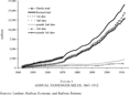
FIGURE 1 ANNUAL PASSENGER MILES, 1843–1912
Time Savings
We assess the value of time saved by combining the data on speeds given in Table 4 (with linear interpolations between benchmark years), and the passenger miles given in Figure 1. We continue our earlier assumptions that those in first and second classes would otherwise have traveled by coach, and that those in third class would otherwise have walked.77
Obviously the further on from the invention of the railways, the harder it is to construct a plausible nonrail counterfactual. Society was richer in 1912 than 70 years before, and some traveling in third class would by then have used the coach rather than walk. Similarly, the bicycle became more practical over time, and fell in price after 1900. The assumption that all third-class passengers would have walked is therefore less likely to be true for 1912 than for earlier. That said, we have already allocated 1.4 billion passenger miles from third to second class—and thus from walking to coach, and even in 1907, after the big price falls, only one bicycle was sold per 75 people in Britain.
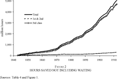
The number of hours saved rose dramatically over the railway era, from 54 million hours in 1843, to 527 million hours in 1866, and finally to 5 billion hours by 1912, roughly equal to the hours worked by 1.8 million workers (see Figure 2). The number of hours saved rises more sharply over time than passenger miles, because over time an increasing proportion of those traveling by train were third-class passengers. Even at the very beginning the third class accounted for over half the hours saved, rising to 80 percent by 1860, and 90 percent by 1880. The Royal Commission was correct: the poorer classes did benefit most in terms of speed.78
Parliamentary Papers: Report from Commissioners: Railways, 1867, vol. 28, part 1, p. liii, paragraph 118.

FIGURE 2 HOURS SAVED NOT INCLUDING WAITING
We now go on to value these hours. For first- and second-class travelers we use an annual wage of £250 in 1911, projected backwards as appropriate. For third-class passengers in 1865 we were fortunate to have Chadwick's direct estimate of their wages. It would not be appropriate, however, simply to index this wage forward. Over the nineteenth century the cost of third-class travel fell relative to workers' wages. Whereas in 1865 workers could travel only 3.3 miles on an hour's earnings, in 1912 they could travel 10.4 miles on an hour's wages. That fall in price relative to earnings would have brought train travel into the reach of more people, although rail travel was still around three times as expensive relative to earnings as it is today. Even today rail travel is used disproportionately by the affluent, so it is again unrealistic to assume that third-class rail travelers would have been a representative cross section of the working class. This conclusion fits with the qualitative literature that notes that railway travel was not used regularly by all sections of the working class.79
Kellett, Railways, chapter 11, has a good discussion of the means of transport—walking, horse drawn omnibus, tram—used by the working class.
The average English person was taking 26 trips per year by the end of the century: such volumes of travel indicate that travelers were people of at least moderate means. Weyl, Passenger Traffic, p. 110.
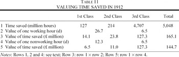
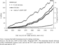
For years before 1865 we use Chadwick's wages, indexed via Feinstein's series; this assumption is less critical given the lower numbers of third-class passengers early on. Table 11 gives the value of the 5 billion hours of time saved assuming first that all travel is in work time and second that none of it is in work time. The estimates range from £145 million to £165 million. As for 1865, neither extreme makes sense, and using the earlier plausible hypothesis that half of premium traffic was for business gives a saving of £155 million, just over 10 percent of England and Wales GDP. Again, it is implausible to believe that fewer than one-quarter or more than three-quarters of premium-class passengers were on business, as such, it is implausible to believe that the correct answer is different to our best guess by more that 3 percent. The exercise is set out for 1912 in Table 11, and the results for all years are given in Figure 3.


FIGURE 3 THE VALUE OF TIME SAVED, 1843–1912
Money Savings
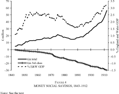
The miles traveled in each year, the railway fares, and the cost of alternative modes of transport found earlier are sufficient to generate the monetary social savings estimates at different dates, which are given in Figure 4. We have assumed that the nature and costs of alternative means of travel would have remained unaltered. It is possible to claim that the cost of coaching would have risen (greater demand for horses, congestion) or that it would have fallen (economies of scale in coach building, better roads), so the assumption of constant prices is reasonable.

FIGURE 4 MONEY SOCIAL SAVINGS, 1843–1912
Figure 1 showed that passenger miles rose 16-fold between 1850 and 1912. Despite this, Figure 4 shows that the money social savings rose only sixfold. As Figure 1 shows, most of the rise in passenger miles was in third-class travel. Even when we exclude the proportion of third-class passengers who would have traveled second class were it to have been offered, we still have a large rise in the number of people who would otherwise have walked. For this group, the money social savings are negative. The increase in fare revenues from third-class passengers partly counteracted the additional savings made by first- and second-class passengers, for whom the money cost of travel fell sharply.
Given that we have imposed a linear fall in the price of tickets between 1865 and 1912, we should not place too much confidence in the pattern of savings between those dates. Our initial starting point in 1865 is sound, and our final observation in 1912 is in line with both Acworth and Stephenson and Cain, but the results in between these two dates must be viewed as an educated guess. It is probably most sensible to see social savings rising to 2.5 percent in the early 1850s, and remaining in that region for the next 50 years.
The Changing Nature and Composition of Social Savings
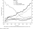
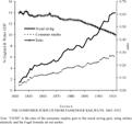
Because we now know both the value of time and money savings for each year between 1843 and 1912 we can calculate the total social saving generated by railways in England and Wales. The three series—time, money, and total—are given in Figure 5. The value of time is based on the earlier plausible assumption that half of premium travel was on business. From 1.5 percent in the early 1840s, the total social saving grew rapidly to reach 4.5 percent by the mid-1850s, before growing reasonably steadily to reach almost 14 percent by 1912. Figure 5 also shows that monetary savings became relatively less important over time, accounting for around two-thirds of the total social saving in the 1840s, falling back to a quarter or below from the mid-1880s onwards. This was the era in which the railway had become primarily a way of saving time rather than saving money. Railways also represent a reasonably steady proportion of (cumulative) TFP growth throughout the period, at around 15 percent. There is no evidence of relative underperformance of British railways productivity growth as the period progressed.

FIGURE 5 THE SOCIAL SAVINGS FROM PASSENGER RAILWAYS, 1843–1912
We noted earlier that the social saving overstates the rise in consumer surplus. If travel costs had been as high in 1912 as they were before railways then far fewer people would have traveled. We set out the formula to convert social savings into consumer surplus above, along with our reasons for preferring unitary elasticity. On that basis we calculate the consumer surplus for each year in our period. As Figure 6 shows, consumer surplus rose steadily, albeit at a slower rate than social savings. The growing divergence reflects the falls in the (generalized) cost of traveling by train: a larger proportion of journeys in 1912 were induced by lower prices than was true earlier in the period when travel was slower and fares were higher. A higher proportion of rail journeys towards the end of the period would thus not have been undertaken without railways: these induced journeys are included in social savings, but excluded from consumer surplus. Nevertheless, consumer surplus rises steadily from 1 percent in 1843 to more than 6 percent in 1912.

FIGURE 6 THE CONSUMER SURPLUS FROM PASSENGER RAILWAYS, 1843–1912
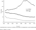
As Figure 5 showed, the ratio of money to total savings fell over time, from three-quarters at the beginning, to one-half in 1866, to one-quarter in 1883, after which it stabilized at between 20 and 25 percent until 1912. The rise in the importance of time relative to money savings reflects the changing nature of the railway in this period. Initially railway companies saw the railway as an alternative to coaching, and offered services that were priced and structured accordingly. But from 1870 onwards, railways became an ever more mass market commodity, whereby train companies often aimed to make a profit by conveying many people, relatively cheaply, at high load factors. We can see this transition in Figure 7, which gives the percentage of total social savings that went to premium-class travelers. This shift towards mass transport may have been a peculiarly British phenomenon; we know that railway penetration was much less extensive in other countries.81
For example, whereas England had 26.5 journeys per capita in the mid 1890s, the figure for France was 9.1, lower than the level reached in England in 1864. France was low even by continental standards, but nonetheless Denmark, Prussia, Netherlands, Saxony, Sweden, and Switzerland all lagged significantly behind England in the number of journeys per head, and thus, almost certainly, in the proportion of people who traveled by train at some point. Ibid., chapters 8 and 9.

FIGURE 7 PROPORTION OF SOCIAL SAVINGS ACCRUING TO PREMIUM CLASS PASSENGERS
Initially premium passengers gained almost all of the benefit—they represented the majority of the traffic, and, at the initial price and speed combinations, third-class passengers did not gain a large amount of surplus per mile traveled. Over time, however, third class became a larger share of total travel, and the rise in speed and fall in prices increased the gain per mile for third-class passengers. As such, the premium passengers' share of gains fell steadily to around one-half from the mid-1890s onwards. When, however, we look at the two different types of saving, very different pictures emerge. The premium-class passengers always gain more than 100 percent of the monetary social saving, because for third-class passengers the railways are more expensive than the alternative. But for time savings the position is very different. Not withstanding that premium passengers' time is valued much more highly per hour, the share of the value of time saved by premium passengers fell sharply from three-fifths in 1843 to around two-fifths by 1850, followed by a steadier decline to one-sixth by 1885, after which it stabilized.
This pattern fits with what we know about technological adoption. In the initial period, new technology is used in the same way as the previous technology. In this case, railways were used to carry the well-to-do in comfort, while conditions for those in the third class were very poor, both in terms of comfort and convenience.82
Bagwell, Transport Revolution, pp. 107–10.
This continued increase in the value of railways to society long after their invention and adoption fits with what we know about other so-called “general purpose technologies.” Paul David has shown how initially electricity had only limited effects on business: it was only when factories reorganized production to take account of the possibility of unit drives that the productivity revolution occurred.83
David, “Computer and Dynamo.”
There is another way in which these findings fit well with the more general literature on technology. William Nordhaus has shown that, on average, postwar American entrepreneurs in the nonfarm sector captured only 2.2 percent of the total benefit to society from new inventions. The remaining 97.8 percent went to consumers as additional consumer surplus.84
Nordhaus, “Schumpeterian Profits.”
Arnold and McCartney, “Rates of Return,” pp. 54–55.
CONCLUSIONS
This article makes a number of contributions. It has calibrated the rise in train speeds prior to 1912, and used those results to assess the additional amount of time that it would have taken to undertake all railway journeys without railways. The numbers are large, and increased rapidly over time: growing tenfold from the mid-1840s to the mid-1860s, and then tenfold again by the outbreak of the First World War, at which point it would have taken an additional five billion hours to undertake all rail journeys without them, using the means of transport that passengers would have chosen in the absence of railways. Trains were much faster than coaches or walking, and became faster over time, with average speeds rising from 20 to 28 miles an hour between 1850 and 1910, or 37 miles an hour on more important routes. Although initially less important than the money savings offered by railways, the value of time saved became as important in the 1860s, and considerably more important thereafter. By the mid-1880s, time savings outweighed money savings by a factor of five.
The social savings from railways, in time and money, amounted to some 2 percent of GDP as early as 1850, to 5 percent of GDP by 1865, 10 percent by the end of the century, and fully 14 percent by 1912. Even when we use the consumer surplus estimate the gains are significant. At the most plausible price elasticity assumption of 1 percent, the consumer surplus benefit from railways represented 6 percent of national income in 1912.
These savings are significant relative to those available from other sources in the nineteenth century. Including the value of time saved by passenger railways increases the total level of TFP growth in the economy by 9 percent, with passenger railways alone accounting for around 15 percent of total TFP growth in the pre-1913 railway era. They were thus a major contributor to aggregate productivity growth in this era.
Railways represented a dramatic change in transport technology. The cost of travel fell significantly, and its speed and comfort rose dramatically. This is particularly true from the 1870s onwards, as railways sought to attract more customers with better third-class services. People who could never have expected to travel at all in their lives were able to do so for the first time. And those who did travel were able to do so more often. This article does not claim to measure all of the benefits of railways to travelers, let alone to the economy or society as a whole. But it does claim to have calculated the social savings and consumer surplus of passenger railways. Those figures show that the contribution of railways relative to national income continued to rise over in the Victorian and Edwardian eras, as rail companies discovered new and better ways to make this technology valuable to society. As the period progressed railways offered poor returns to investors, but they delivered tremendous welfare gains to travelers and to society.
Appendix
50 IMPORTANT ROUTES
Birmingham-Dudley, Leeds-Bradford, Liverpool-Birmingham, Liverpool-Leeds, Liverpool-Preston, Liverpool-Sheffield, London-Bath, London-Birmingham, London-Bradford, London-Brighton, London-Bristol, London-Cambridge, London-Canterbury, London-Cardiff, London-Chatham, London-Colchester, London-Coventry, London-Derby, London-Dover, London-Hull, London-Ipswich, London-Leeds, London-Leicester, London-Liverpool, London-Maidstone, London-Manchester, London-Newcastle, London-Northampton, London-Norwich, London-Nottingham, London-Oldham, London-Oxford, London-Plymouth, London-Portsmouth, London-Preston, London-Reading, London-Sheffield, London-Southampton, London-Wolverhampton, Manchester-Birmingham, Manchester-Blackburn, Manchester-Bolton, Manchester-Bradford, Manchester-Leeds, Manchester-Liverpool, Manchester-Macclesfield, Manchester-Oldham, Manchester-Preston, Manchester-Sheffield, Manchester-Stockport
222 TOWNS AT WHICH MINOR JOURNEYS ENDED
Abergavenny, Alderley Edge, Alfreton, Altrincham, Andover, Ashford, Ashton-under-Lyne, Barnsley, Barnstaple, Barrow, Barry, Basingstoke, Bath, Bedford, Berwick, Beverley, Birkenhead, Birmingham, Blackburn, Blackpool, Blyth, Bolton, Bournemouth, Bradford, Bridgnorth, Bridgwater, Bridlington, Brighton, Bristol, Bromsgrove, Burnley, Burslem, Burton on Trent, Bury, Buxton, Cambridge, Cardiff, Carlisle, Carnarvon, Castleford, Caterham, Chatham, Chelmsford, Cheltenham, Chertsey, Chester, Chesterfield, Chichester, Chorley, Cirencester, Clevedon, Coalville, Colchester, Colne, Colwyn Bay, Conway, Coventry, Cowes, Crewe, Darlington, Dartford, Dartmouth, Darwen, Denton, Derby, Dewsbury, Doncaster, Dorchester, Dover, Driffield, Dudley, East Grinstead, Eastbourne, Eccles, Exeter, Felixstowe, Fleetwood, Folkestone, Garston, Gateshead, Glossop, Gloucester, Grantham, Gravesend, Grimsby, Halifax, Hanley, Harrogate, Hartlepool, Hastings, Hereford, Heywood, Hinckley, Huddersfield, Hyde, Ilkeston, Ipswich, Jarrow, Keighley, Keswick, Kettering, Kidderminster, Kings Lynn, Kingston upon Hull, Kingswood, Kirkby Lonsdale, Lancaster, Leamington, Leeds, Leek, Leicester, Leigh, Leighton Buzzard, Lewes, Leyland, Lichfield, Lincoln, Liverpool, Llandudno, Llanelly, London, Long Eaton, Longton, Loughborough, Lowestoft, Luton, Lyme Regis, Macclesfield, Maidstone, Malvern, Manchester, Mansfield, Margate, Merthyr Tydfil, Middlesbrough, Middleton, Mirfield, Nantwich, Newark, Newcastle, Newcastle under Lyme, Newmarket, Newport, North Shields, Northampton, Northwich, Norwich, Nottingham, Nuneaton, Oldham, Oxford, Padiham, Peterborough, Plymouth, Pontypool, Pontypridd, Portsmouth, Preston, Radcliffe, Ramsgate, Reading, Reigate, Rochdale, Rochester, Rodwell, Rotherham, Rugby, Runcorn, Sale, Scarborough, Seaford, Selby, Sheffield, Shipley, Shrewsbury, Sleaford, Smethwick, South Shields, Southampton, Southport, Sowerby Bridge, St Annes, St Helens, St. Albans, St. Austell, Stafford, Stalybridge, Stockport, Stockton-on-Tees, Stoke on Trent, Stroud, Sunderland, Sutton Coldfield, Tamworth, Taunton, Tewkesbury, Torquay, Tredegar, Tunbridge Wells, Tunstall, Ulverston, Wakefield, Wallasey, Wallsend, Walsall, Warrington, Warwick, Watford, Wellingborough, West Bromwich, Weston super Mare, Widnes, Wigan, Wilmslow, Windermere, Wisbech, Woking, Wolverhampton, Worcester, Wrexham, Yarmouth, York
In his Economic History Association Presidential Address, Fogel wrote that “Scientific creations, however, are usually protracted over long periods, approach perfection quite gradually, and involve the efforts of a large number of investigators. The social savings controversy has demonstrated the great complexity of the analysis of the developmental impact of railroads, the wide range of issues that need to be pursued, the large amounts of data that must be retrieved and the many pitfalls that may be encountered in the analysis of these data. Such problems are resolved through collective effort” (“Notes,” p. 51). Where this article alters the existing literature it does so in that spirit of collective effort. I thank Dudley Baines, Dan Bogart, Nick Crafts, Terry Gourvish, Peter Mackie, Abay Mulato, the Editor, three excellent referees and seminar audiences at the Berlin Quantitative Economic History Colloquium, Economic History Society Conference, Linköping University, LSE, Oxford University, and the U.K. National Rail Museum for helpful comments, and my first rate research assistant, Judith Allen, for the unenviable task of entering all of the railway and coaching timetable data. Funding from the ESRC, under grant R000239536, is gratefully acknowledged. All remaining errors remain my own.