In many settings, political scientists wish to test theories where they must confront two distinct data challenges: (1) there is often an excess of zeros in the outcome variable, and (2) the data-generating process for multiple outcomes may be related. This is particularly true when studying-related decisions between political actors who must allocate scarce resources. For instance, consider the decision-making processes of competing parties regarding candidate visits during a presidential campaign. In practice, these campaigns can only visit a small proportion of localities within a country during a single campaign. (The outcome exhibits an excess of zeros.) Thus, many municipalities are never considered worthwhile for visits by any candidate due their small populations or non-competitive nature. To make things more complicated, however, of those municipalities that are worthwhile to (potentially) visit, decisions by campaigns are also interdependent. That is, parties may visit municipalities simply because they anticipate that they will be visited by their opponents, or actors may make decisions based on similar but unobserved factors.
Ignoring either of these issues—zero-inflation and interdependence—can bias parameter estimates and decrease the efficiency of the estimators. Furthermore, by failing to address them, we miss an opportunity to better understand important features of the data-generating process. What factors are related to being either a unit that is considered for resource allocation or excluded completely? Is there really evidence that the behavior of one actor is related to, or even shaped by, the (anticipated) behavior of other actors? Finally, do different actors respond heterogeneously to different factors?
In this paper, I extend the zero-inflated ordered probit (Harris and Zhao Reference Harris and Zhao2007) to better address these issues by allowing for interdependent multivariate outcomes, developing a zero-inflated multivariate ordered probit (ZIMVOP). It consists of two steps. The first step models the observation as a potential non-zero, splitting the population into “always zeros” and “potential non-zeros.” The second step is a multivariate ordered probit, allowing correlations of the disturbance terms across equations over dimensions.
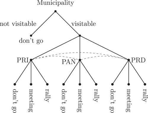
To make this model more concrete, and to provide a running example, I re-analyze a data set of Mexican presidential campaign visits in 2006 and 2012 for the three major parties—the Partido Revolucionario Institucional (PRI), the Partido Acción Nacional (PAN), and the Partido de la Revolución Democrática (PRD) (Langston and Rosas Reference Langston and Rosas2016). The outcome of interest is the level of visitation by each of the parties—no visit, hold a meeting, or hold a rally. Because there are three parties, the outcome is trivariate. In other words, each municipality has three outcomes, one for each party, that are inherently related. Further, the vast majority of the municipalities were never visited by any party. Figure 1 provides a graphical depiction of the parties’ decisions.
Parties’ decision trees Note: The decision of a party is split into two steps. The first decision is whether or not a municipality is visitable. The second decision is the type of visit, conditional on the municipality being visitable. This decision is likely related to the decisions of other parties. PRI=Partido Revolucionario Institucional; PAN=Partido Acción Nacional; PRD=Partido de la Revolución Democrática.

Unfortunately, no current model can accurately capture the decision tree described. Zero-inflated models cannot measure the extent of interdependence between parties’ decisions. Models allowing correlations between outcomes (e.g., seemingly unrelated regressions (SUR)) would not capture the zero-inflation. Both approaches are inefficient and could lead to inaccurate estimates and potentially incorrect conclusions. The contribution of this paper, therefore, is to provide a model that can correctly account for both zero-inflation and interdependence to allow political science researchers to better understand these kinds of processes.
ZERO-INFLATED AND CORRELATED ERRORS: ISSUES AND SOLUTIONS
In this section, I discuss the issues associated with outcomes that exhibit an excess of zeros and current approaches to dealing with these issues. I then do the same for multivariate models that have correlated error terms, known as SUR. Neither of these families of models adequately addresses the problems of both zero-inflated outcomes and correlated error terms. Through the discussion, I highlight the advantages to current approaches and demonstrate that ZIMVOP, a synthesis of the two families of models, is an intuitive extension when dealing with data that raise both of these concerns.
Models with Zero-Inflation and SUR
King and Zeng (King and Zeng Reference King and Zeng2001a; King and Zeng Reference Nieman2001b) introduce a unique approach to modeling rare outcomes, focusing primarily on international conflict. They argue that modeling conflict on all country dyads underestimates the effect of certain factors, producing biased estimates. This is due to the fact that the vast majority of dyads will never go to war, regardless of certain observed characteristics that may actually be deterministic in other dyads. The approach they suggest is to save data collection, maintain all non-zero observations in the data, randomly sample zero outcomes, and focus more time on the quality of the data than the quantity of data.
This recommendation saves data collection and may lead to less biased estimates relative to running a standard probit on lower-quality data. However, observed zeros may have distinct data-generating processes, suggesting a split-population approach (Harris and Zhao Reference Harris and Zhao2007). This split-population method differs from the rare events method by modeling the outcome in two steps. The first step models the probability that an observation is a potential non-zero, and the second step models the outcome conditional on the observation being a potential non-zero. The split-population refers to splitting the population into “potential non-zeros” and “always zeros.” An intuitive example relates to civil conflict. Bagozzi et al. (Reference Bagozzi, Hill, Moore and Mukherjee2015), using a zero-inflated ordered probit, find that a country’s gross domestic product has a reliable and negative effect on the potential for political violence, but on a potential non-zero, the effect is positive. That is, rich countries are less likely to experience political violence, but on a potential non-zero, income has a positive effect on the outcome, likely due to greater resources.
This example highlights both the issues related to ignoring an excess of zeros and the benefits in addressing them. If the two steps were ignored, the nuanced effects of these covariates would be lost and the estimates of the effects would be biased, because a standard model with no inflation would lead to a correlation between the error terms and the explanatory variables (Bagozzi and Marchetti Reference Bagozzi and Marchetti2014; Dunne and Tian Reference Dunne and Tiann.d.).
In addition to the problems associated with an excess of zeros, outcomes also may share related data-generating processes. The SUR class of models stacks regressions and allows the error terms across these stacked regressions to be correlated (Zellner Reference Zellner1962). Jointly estimating a set of equations improves asymptotic relative efficiency over the equation-by-equation case by combining information across equations (Zellner and Huang Reference Zellner and Huang1962; King Reference King1989). In other words, in the limit, the estimators produce estimates with smaller mean squared errors and smaller variances.
Partial Observability in Strategic Settings
The ZIMVOP model I propose below seeks to combine the approaches above in order to achieve three simultaneous goals: (1) understand the relationship between the main explanatory variables and the outcome; (2) understand the process that leads some observations to be excluded from consideration; and (3) detect inter-dependencies in the data-generating process for multiple outcomes. While several of the models above can achieve one or two of these goals, none can accomplish all three simultaneously.
Nonetheless, it is important to note that there are several other models in the literature that are similar in important ways to my own. Gurmu and Dagne (Reference Gurmu and Dagne2012) developed a zero-inflated bivariate ordered probit, but it does not easily extend to the multivariate case (see also Kadel Reference Kadel2013).Footnote 1 ZIMVOP generalizes this zero-inflated ordered probit to have a theoretically unbounded number of dimensions in an intuitive, straight-forward manner.
Another project for settings with partially observable outcomes is presented by Nieman (Reference Nieman2015), who proposes a model for strategic interactions in a two-player, sequential game. Similar to ZIMVOP, we observe the same outcome from two distinct data-generating processes (status quo or government acquiesces). Despite the seeming similarity, the underlying behavior modeled by ZIMVOP and Nieman are quite distinct, with the former estimating related decision-making or processes, and the latter modeling a strategic game.
ZIMVOP SPECIFICATION
ZIMVOP has two major components that in combination set the model apart from current approaches. The first is a zero-inflation step. This is simply a univariate standard probit that models the probability that an observation is a potential participator, or a potential non-zero. In the Mexico example, this is whether or not any party will even consider visiting a given municipality. This follows the zero-inflated ordered probit approach developed by Harris and Zhao (Reference Harris and Zhao2007).
The second component is a multivariate ordered probit for the final outcomes. For each observation, there is a vector of outcomes, one scalar outcome for each dimension. In the Mexico example, the “dimensions” are each party, one dimension for the PRI, one for the PAN, and one for the PRD. Each observation is a municipality in a given time period, and the outcome is a vector of length three, with one outcome for each party. The outcome for each component takes one of three values: 0 for no visit, 1 for a meeting, and 2 for a rally. In this step, conditional on being a potential non-zero (e.g., a visitable municipality), an ordered outcome is modeled separately for each dimension, but the error terms are allowed to correlate across dimensions (parties). In other words, the decision processes at the second step for each party are not assumed independent in a given municipality and time period.
In presenting the model, I follow the presentations of Harris and Zhao (Reference Harris and Zhao2007), Gurmu and Dagne (Reference Gurmu and Dagne2012), and Kadel (Reference Kadel2013). This set-up requires that we model the observed outcome for unit i on dimension r, y ri , as the product of two unobserved discrete latent parameters, y ri =s i z ri , where s i indicates whether unit i is a potential non-zero, and z ri the estimated level of outcome conditional on observation i being a potential non-zero. In our Mexico example, s i ∈{0, 1} represents whether a municipality is “visitable” by one of the parties, while z ir ∈{0, 1, 2} is the model’s estimate of whether there will be no visit (0), a meeting (1), or a rally (2) by party r in that municipality.
First Step
Both the first-step probit and the second-step multivariate ordered probit follow Albert and Chib’s (Reference Albert and Chib1993) data augmentation approach such that we include in our model latent parameters. Sampling of latent parameters leads to probability distributions for the observed outcomes, and significantly improves computational tractability.
Let
 $$s_{i}^{{\asterisk}} $$
be a latent parameter capturing the potential for observation i to be a non-zero (visitable) observation such that the probability of i being a non-zero is equal to
 $$\:{\rm Pr}\:\left( {s_{i}^{{\asterisk}} \,\gt\,0} \right)$$
. This latent value is modeled as a linear function of a matrix of covariates, V, with each row, v
i
, being a vector of observation-level covariates (including a constant). Specifically, we let
 $$s_{i}^{{\asterisk}} {\equals}{\bf v}_{{i'}} \gamma {\plus}\mu _{i} $$
, where γ is a vector of unknown parameters to be estimated and µ
i
the error term such that μ
i
∼N(0, 1).Footnote
2
Now, let s i , the latent categorical parameter indicating potential non-zero observations, be defined as:
 $$s_{i} {\equals}\left\{ {\matrix{ 0 & {{\rm if}\,s_{i}^{{\asterisk}} \leq 0,} \cr 1 & {{\rm if}\,s_{i}^{{\asterisk}} \,\gt\,0.} \cr } } \right.$$
Let Φ(·) denote the normal cumulative distribution function. Then
 $${\rm Pr}\left( {s_{i} {\,\equals\,}1} \right){\,\equals\,}\Phi \left( {s_{i}^{{\asterisk}} } \right){\,\equals\,}\Phi \left( {{\bf v}'_{{i'}} \gamma } \right),$$
is the probability of the observation being a potential non-zero.
Second Step
In the second step, let r=1, … , D, where D is the total number of dimensions. The Mexico example has a trivariate outcome (D=3), with r equal to 1, 2, and 3, each number indicating a party. Again following the standard data augmentation approach, let
 $$z_{{ri}}^{{\asterisk}} $$
be the latent parameter related to the outcome level for observation i on dimension r conditional on observation i being a potential non-zero. These levels of participation for the Mexico parties are, in order: do not go (0), go for a meeting (1), or go for a rally (2). Let X
r
be a n by p matrix of predictors for the level of participation on dimension r (which includes a constant). Let the n by p by D array of all second-step predictors for all dimensions be denoted
 $${\cal X}$$
. We let
 $$z_{{ri}}^{{\asterisk}} {\equals}{\bf x}'_{{ri}} \beta _{r} {\plus}{\epsilon}_{{ri}} $$
, where ε
ri
is the error term and β
r
the unknown vector to be estimated for dimension r.
Our goal is to estimate the latent categorical parameter z ri , which is the level of participation for observation i on dimension r conditional on being a potential non-zero. In the data augmentation approach, to allow for multiple categories, we need to also estimate a vector of “cut-off” parameters (Albert and Chib Reference Albert and Chib1993). Let a r be the vector of cut-off points of length j r , where j r is the maximum possible outcome on dimension r (in our example j r =2 for all r), and a rk the k th cut-off on dimension r. We can now define z ri as:
 $$z_{{ri}} {\equals}\left\{ {\matrix{ {0\quad {\rm if}\quad z_{{ri}}^{{\asterisk}} \leq a_{{r1,}} } \cr {k\quad {\rm if}\quad a_{{rk}} \,\lt\,z_{{ri}}^{{\asterisk}} \leq a_{{rk{\plus}1}} ,} \cr {j_{r} \quad {\rm if}\quad z_{{ri}}^{{\asterisk}} \,\gt\,a_{{rj_{r} {\minus}1}} .} \cr } } \right.\quad k{\,\equals\,}1,\,\ldots\,,j_{r} {\minus}1,$$
Critically, in the second step we want to allow the error terms to be correlated.Footnote
3
We therefore let the vector of error terms across dimensions, ε
i
, be distributed multivariate normal with mean 0
D
, a vector of zeros of length d, with variance–covariance matrix ∑
D
:
 $${\epsilon}_{i} \,\sim\,{\cal N}_{D} \left( {{\bf 0}_{D} ,{\mib S}_{D} } \right)$$
. Finally, we model the observed vector of outcomes for a municipality, y
ri
as the product s
i
z
ri
.
Likelihood
In the likelihood function that follows, allow i to index observations. Let Y denote the matrix of observations for all dimensions. To write the likelihood for any number of dimensions and because the outcomes are not assumed independent, we must let g index the vectors of potential outcomes. Let I(z i =g) be an indicator function as to whether the observation is equal to g. For example, to simplify the likelihood, consider the probability of different outcomes in the trivariate case. A zero outcome on three dimensions would be the probability that s i =0 added to the probability that s i =1 multiplied by the probability of all outcomes equaling zero (g would be equal to [0, 0, 0]): Pr( y i =[0, 0, 0])=Pr(s i =0)+Pr(s i =1)×Pr(z 1i =0,z 2i =0,z 3i =0). An outcome of, for example, [1, 0, 2], would be: Pr(s i =1)×Pr(z 1i =1,z 2i =0,z 3i =2). The likelihood function for any number of dimensions is
 $$\eqalignno{ & {\scr L}\left( {{\bf Y}\,\mid\,{\cal X},{\bf V},\beta _{1} ,\,\ldots\,,\beta _{D} ,\gamma ,{\bf a}_{1} ,\,\ldots\,,{\bf a}_{D} ,{\bf s},{\bf Z}} \right){\equals} \cr & \quad \prod\limits_{i{\equals}1}^N \left( {\prod\limits_{{\bf g}{\equals}{\bf 0}} \left[ {{\rm Pr}\left( {s_{i} {\equals}0} \right){\plus}{\rm Pr}\left( {s_{i} {\equals}1} \right){\rm Pr}\left( {{\bf z}_{i} {\equals}{\bf g}} \right)} \right]^{{{\rm I}({\bf z}_{i} {\equals}{\bf 0})}} } \right. \cr & \quad \left. {{\times}\prod\limits_{{\bf g}\,\ne\,{\bf 0}} \left[ {{\rm Pr}\left( {s_{i} {\equals}1} \right){\rm Pr}\left( {{\bf z}_{i} {\equals}{\bf g}} \right)} \right]^{{{\rm I}({\bf z}_{i} {\equals}{\bf g})}} } \right). $$
Now that I have specified the model’s two-step process and the generalized likelihood, I will discuss the prior distributions for the parameters of interest to fully specify ZIMVOP.
Priors
Let the first-step error terms, μ
i
, follow the normal distribution with mean 0 and SD 1:
 $$\mu _{i} \,\sim\,{\cal N}(0,1)$$
. In frequentist statistics, setting the SD to 1 is necessary to identify the model (Cameron and Trivedi Reference Cameron and Trivedi2005). Though in a Bayesian context we could put a hyperprior on the variance, I choose not to in order to make the model easier to interpret and to hasten convergence.
The precision matrix
 $$\sum_{d}^{{{\minus}1}} $$
is distributed inverse-Wishart with the d×d identity matrix as the mean and degrees of freedom ν:
 $$\sum_{d}^{{{\minus}1}} \,\sim\,{\scr I}{\cal W}\left( {{\bf I}_{d} ,\nu } \right)$$
.Footnote
4
Because the variance is unconstrained in the specification, two cut-offs along each dimension are set to identify the model.Footnote
5
By setting two cut-offs rather than just one at zero, the variance along each dimension is identified. Set a
r1 to 0 and a
r2 to some positive constant c
r
for each dimension. We can let all undefined a
rk
follow a log-normal distribution with mean 0 and variance σ
2:
 $$a_{{rk\,\gt\,2}} \,\sim\,\ln {\cal N}(0,\sigma ^{2} )$$
. Note that no order is imposed on these cut-offs. In our trivariate Mexico example, there are only two cut-offs, which are both defined as constants, so this choice in prior is for generalizability only and is not implemented in the application. Finally, we let our coefficients, γ and β
1:d
, have diffuse normal priors centered at zero. The model is written in JAGS and the code is provided in the Supplementary Information Section SI-1. Note that these priors can be changed to meet the needs of a particular data analysis, but this subsection, aside from specifying how I choose to set the priors, highlights the considerations necessary.
APPLYING ZIMVOP
This section first shows illustrative examples on simulated data to demonstrate the problems that can arise when researchers ignore the zero-inflation or the correlations in the underlying data-generating processes. I then apply the model to presidential campaigns in Mexico.
Implementation on Simulated Data
ZIMVOP synthesizes zero-inflation and SUR models. To isolate the gains of ZIMVOP in comparison to either models not accounting for zero-inflation or not accounting for correlated errors, I perform two sets of simulation exercises. The first set compares ZIMVOP to a multivariate ordered probit without zero-inflation, varies the degree of zero-inflation, and does not impose a correlation on the generated error terms. The second set compares ZIMVOP to an unpooled (i.e., separate equations for each dimension) zero-inflated probit, varies the correlation of the error terms, and does not vary the degree of zero-inflation.Footnote 6 By performing these simulation exercises separately, as opposed to comparing all three models on the same sets of data, I can set-up the data to make the competing model better able to capture the parameters of interest, allowing for a harder test of ZIMVOP.
Simulation exercise I: zero-inflation
The first set of simulations compare ZIMVOP to a model without the zero-inflation step, a multivariate ordered probit (a SUR model). Data are generated through eight different zero-inflated processes. The generation of the data involves a zero-inflation step with an intercept (γ 0) of −1.5 and a coefficient (γ 1) changing from 4 to 11 by increments of one.Footnote 7 The first-step equation is therefore:
 $$\eqalignno{ & s_{i}^{{\asterisk}} {\equals}{\minus}1.5{\plus}v_{i} {\times}\gamma _{1} {\plus}\mu _{i} , \cr & \mu _{i} \,\sim\,{\cal N}\left( {0,1} \right), {\rm and} \cr & s_{i} {\equals}\left\{ {\matrix{ 0 & {{\rm if}\,s_{i}^{{\asterisk}} \leq 0,} \cr 1 & {{\rm otherwise}.} \cr } } \right. $$
The first-step variable of interest is a single vector, v, of length 500, drawn randomly from a standard normal. For each simulation analysis, these data are resampled in this manner, but I analyze each unique data set by the competing models to ensure comparability. These data are not nested in the second-step variables, which are independently generated. This is a harder test than nesting the values, because some of the variation of the zero-inflation step should be accounted for in the second-step intercept estimates, and much of it could be accounted for by the modeled correlation. In other words, if the zero-inflation step is unmodeled, the second-step estimates can in theory predict reasonable non-zero outcomes, and use the correlation and variance of the error terms to explain the excess zeros not following the pattern of the second step.
The second step consists of three levels of outcome on three dimensions. In generating the outcome, the intercept term on each dimension is set to 0, and the three dimensions each have one predictor, set to 2, 2.5, and 2. The second-step equation is therefore:
 $${\bf z}_{i} {\equals}{\bf x}_{{\bf i}} \left( {\matrix{ 2 \cr {2.5} \cr 2 \cr } } \right)'{\plus}{\epsilon}_{i} ,\quad {\epsilon}_{i} \,\sim\,{\cal N}\left( {{\bf 0}_{3} ,{\bf I}_{3} } \right).$$
The cut-offs for every dimension are set to 0 and 2. To demonstrate only the issues arising from not modeling the inflation, all correlations are set to 0, meaning the random errors used to generate the outcome are completely independent. This further allows the first step to be captured by the correlation estimates, acting as an observation-level random effect. The matrix X is a 500×3 matrix of random draws from the standard normal, with a column for each dimension. Again, these are redrawn for each simulation, but I analyze each unique data set by both models. These simulations are repeated 100 times for each of the γ 1 values, for a total of 800 sets of data and 1600 analyses.Footnote 8
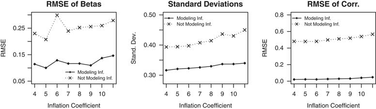
Despite the difficulty of the test, Figure 2 shows that across specifications, the model accounting for the zero-inflation performs better. The root mean squared error (RMSE),Footnote 9 a measure of bias and inefficiency, of the second-step estimates is smaller, while the standard deviations, a measure of precision, of the posteriors are smaller. The average bias across specifications is very close to 0 for both models, suggesting that in the aggregate neither has an expectation of bias, but, as shown by the relatively high RMSE, any given estimate using the MVOP estimator is much less likely to be close to the true value of interest. Further, the estimation of the correlation is much closer to the true values when modeling the zero-inflation. If we have a substantive interest in the correlations, we will get very biased results if we do not account for zero-inflation. Finally, across all simulations and specifications, the coverage probability in the model with a first step is 0.92, while the model without the first step is 0.86.Footnote 10 This suggests that the decrease in standard errors is not leading to overly restrictive posteriors.
Results of the simulations varying the degree of zero-inflation Note: The panel on the left shows the root mean squared error (RMSE) of the second-step estimates as the first-step zero-generating coefficient is increased from 4 to 11. The RMSE is larger for the models without a first step. The middle panel shows the standard errors of the second-step posterior estimates. The standard errors are always larger for the model without a first step. The right panel shows the RMSE of the correlation estimates for the two models. The model without a first step always has much greater RMSE and it increases with the inflation coefficient.

Simulation exercise II: correlated error terms
The second set of simulation exercises compares a ZIMVOP model with second-step correlated errors to the same model not allowing correlations. The simulations again generate data with a zero-inflation process, but vary the correlations of the second-step error terms. The true data-generating process sets the first-step intercept, γ 0, to −1.5. The single coefficient of interest in the first step, γ 1, is set to nine. The first-step equation is therefore:
 $$\eqalignno{ & s_{i}^{{\asterisk}} {\equals}{\minus}1.5{\plus}v_{i} {\times}9{\plus}\mu _{i} , \cr & \mu _{i} \,\sim\,{\cal N}\left( {0,1} \right), {\rm and} \cr & s_{i} {\equals}\left\{ {\matrix{ 0 & {{\rm if}\,s_{i}^{{\asterisk}} \leq 0,} \cr 1 & {{\rm otherwise}.} \cr } } \right. $$
The values of v, which is of length 500, are again all drawn from the standard normal for each simulation, and each unique data set is analyzed by the competing models to ensure comparability. The values of the predictors are generated independently of the second-step values, which are generated as above, from a standard normal. They are not nested.
The second step has three outcome levels on each of three dimensions. The coefficients used are the same as the earlier round of simulations. Intercepts are set to 0 and the parameters of interest are set to 2, 2.5, and 2. The outcomes generated, however, are determined using correlated error terms, with the correlation varying across simulations.Footnote 11 The second-step equation is
 $$\eqalignno{ & {\bf z}_{i} {\equals}x_{i} \left( {\matrix{ 2 \cr {2.5} \cr 2 \cr } } \right)^{\prime} {\plus}{\epsilon}_{i} , \cr & {\epsilon}_{i} \,\sim\,{\cal N}\left( {\left( {\matrix{ 0 \cr 0 \cr 0 \cr } } \right),\left( {\matrix{ 1 & {\rho _{{12}} } & {\rho _{{13}} } \cr {\rho _{{12}} } & 1 & {\rho _{{23}} } \cr {\rho _{{13}} } & {\rho _{{23}} } & 1 \cr } } \right)} \right). $$
Again, the cut-offs for every dimension are set to 0 and 2. These simulations are repeated 100 times each, resulting in 2700 sets of data, analyzed once by each model.
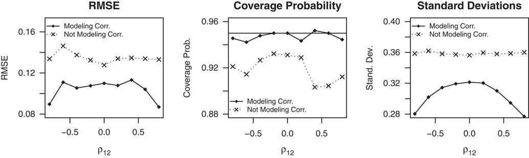
Results of the exercise are shown in Figure 3, pooled by the first correlation coefficient. Again, we see a smaller RMSE in the second-step estimates with tighter posteriors as shown by the smaller standard deviations. The average bias across estimators is very close to 0, but any given estimate is less likely to be close to the true value of interest if ignoring the correlations in the error terms, as shown by the high RMSE. Despite the increase in precision, the average coverage probability is still close to 0.95. Further, the ZIOP does not produce correlation estimates, which are substantively interesting, for example, to capture the relationship between parties’ decisions.
Results of the simulations varying correlations Note: The panel on the left shows the root mean squared error (RMSE) of the second-step estimates as the first correlation coefficient increases. The model allowing correlation performs better by this metric. The middle shows the coverage probability of the second-step estimates, with a line at 0.95. The right panel shows the standard deviations of the posterior distributions. Despite the decent coverage of the model allowing correlations, the standard deviation of the posterior distribution is markedly smaller, performing best when the absolute correlations are high.

When comparing the proposed model to both one not modeling the zero-inflation and one not modeling correlations, the proposed model outperforms these currently extant alternatives. Results hold across various specifications and different benchmarks. Overall, the RMSE of the second-step estimates is reduced, and the posterior densities are more precise while still maintaining approximately 0.95 coverage. ZIMVOP is more accurate, more efficient, and produces substantively interesting results by modeling both the zero-inflation step and the second-step correlations.
Application: Presidential Campaigns in Mexico
Having demonstrated the benefits to our inferences using ZIMVOP, I will now apply it to presidential campaigns in Mexico. Langston and Rosas (Reference Langston and Rosas2016) argue that municipal-level party support and competitiveness are significant determinants to party campaigns’ calculi when deciding which municipalities to visit, and whether that visit is a meeting or a rally. Visits can help assess and signal local party strength and their mobilization networks, and can signal a party’s interest in a locality. If they hold a rally and it is not well-attended, however, this can impose more costs than benefits, signaling a lack of strength in the area. Rallies are also expensive, and if the return is not great enough the cost is not worth it. To test the saliency of certain factors entering into this decision, they analyze the Mexican presidential campaigns of 2006 and 2012, focusing on the three major parties—the PRI, the PAN, and the PRD, using a pooled zero-inflated ordered probit.
The current analysis builds on this with two main propositions: (1) the strategies of parties are not the same and will respond to local support differently, and (2) the decisions made by parties are related. Parties likely engage in a Colonel Blotto-type interaction, targeting the municipalities their rivals are targeting,Footnote 12 and their decisions are likely interdependent based on unobservable characteristics as well. ZIMVOP is uniquely suited to test these propositions because coefficient estimates vary between parties, and the correlation between the parties’ decision processes captures the degree to which parties decisions are related. This proposed relationship between the parties should result in a positive estimate of the correlation. Further, the vast majority of municipalities are never visited. To obtain reliable estimates of the correlations between parties’ calculi and the coefficients of interest, a zero-inflation step is necessary.
The outcome is a vector of ordered party outcomes—0 for no visit, 1 for a meeting, and 2 for a rally. There are three dimensions, one for the PRI, one for the PAN, and one for the PRD. For example, if the PRI holds a meeting in a municipality at a given time period, the PAN do not visit, and the PRD hold a rally, the outcome would be [1, 0, 2]. The first-step predictors consist of one matrix of municipal characteristics. I use three variables: Population size, Vote Herfindahl–Hirschman index (HHI), and 2012 dummy. The variable Population size is a measure of how populated a municipality is. Sparsely populated municipalities are not worth a visit. The variable 2012 dummy is a dummy variable indicating if the observation is in 2012 rather than 2006. The visits are, according to Langston and Rosas (Reference Langston and Rosas2016), a common strategy in newer democracies that still have clientelistic networks. As a state’s democracy grows and evolves, these visits should be less common. Finally, to capture competitiveness, I include the HHI of the previous vote as a general measure for party dominance in the municipality. This measure is a sum of the squared previous vote shares for each of the three parties. When it is high, it indicates one party has dominance over the others. These municipalities should be less appealing for parties to visit. Either it is the dominating party and there is little to be gained from a visit, or it is the weaker party and going would be both a waste of resources and potentially damaging.
The second step includes all of the variables used in Langston and Rosas (Reference Langston and Rosas2016), including the first-step variables. Variables included that are not in the first step are Gira, Concurrent, Coparty mayor, and Previous vote. The variable Gira is a dummy variable for whether or not the visit was part of a multi-stop tour. The variable Concurrent is a dummy indicating whether or not the mayoral race is concurrent with the presidential race. The two main variables of interest are Coparty mayor, an indicator for whether or not there is a mayor of the same party, and Previous vote, the party’s previous vote share. These capture the underlying political support for a party. In the original data, if a party visits a municipality more than once in a given time period it is included twice. For this analysis, to keep the number of observations the same and to not falsely give parties 0 outcomes or repeated outcomes, duplicates are dropped, keeping the highest outcome. This only affects about 150 out of over 3000 observations. About half of the data are randomly selected municipalities that were not visited by any party.
Analysis
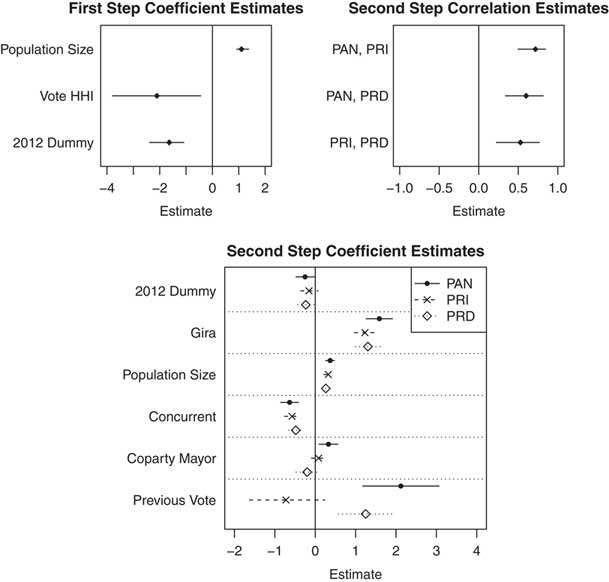
The results of the analysis are presented graphically in Figure 4.Footnote 13 There is strong evidence for the two propositions. First, the correlation estimates are all positive and reliable. This suggests parties are engaging in Colonel Blotto dynamics and targeting municipalities their competitors also target, and that municipalities have unobserved attributes that make them more or less attractive to parties. Second, the second-step estimates for the parties of the variables of interest vary considerably. The estimates for Coparty mayor and Previous vote vary across parties, suggesting different calculi for the parties.
Results from the presidential campaign visits in Mexico Note: Estimates are shown with 95 percent credible intervals of the posterior distribution. The top-left panel shows the first-step estimates. All are reliable and in the predicted direction. The top-right panel shows the correlations between parties in the second step. All are reliable and positive, suggesting parties target municipalities that their competitors target. The bottom panel shows the second-step estimates. The variables of interest, Coparty mayor, and Previous vote vary considerably in their estimated effects, indicating that parties strategize differently. HHI=Herfindahl–Hirschman Index; PRI=Partido Revolucionario Institucional; PAN=Partido Acción Nacional; PRD=Partido de la Revolución Democrática.

For the PAN, having a mayor of the same party reliably increases the odds ratio of moving up a category in the visitation scheme. It is unreliable for the PRI, but indicates that the PRD may be responding to this in the opposite direction. The estimates for Previous vote suggest something similar: parties are not responding in the same way to the same factors. Again, the PAN seem to go where they have support, but so do the PRD, while the PRI estimate, though (just barely) unreliable at a 95 percent level, suggests that the PRI is more likely to visit and hold rallies in municipalities with less support.
Langston and Rosas (Reference Langston and Rosas2016) find that Coparty mayor has a positive effect, while they fail to reject the null that Previous vote has any effect. This is somewhat of an unfair comparison, as they test a generalizable pattern on pooled data, but at the same time this highlights the advantage to allowing actors to respond to factors differently. Perhaps a fairer test is to compare these results to a model not allowing correlation, but allowing the second-step estimates to vary, as in the second simulation exercise. The first-step estimates are nearly identical, but the second-step posteriors are fairly different, with the estimate for previous vote of the PRI no longer reliable even at the 90 percent level. The second-step estimates from both models are compared in Supplementary Information Section SI-3. Perhaps most importantly, we are losing the ability to draw substantive conclusions from the correlations in the latter model. Further, the simulation exercises suggest we should trust the posteriors from ZIMVOP.
CONCLUSION
Binary and ordered outcomes are often of interest in political science, but analyses of these data can be problematic. There is often an excess of zeros, and the data-generating processes of seemingly unrelated outcomes may in fact be related. These issues can lead to inaccurate and inefficient estimators. This paper proposes a new extension to existing models, ZIMVOP, that appropriately addresses these issues and in doing so opens the door to answering questions we have been unable to answer. ZIMVOP not only provides better estimates of our parameters of interest as shown in the simulation exercises, it also helps us recover useful information that otherwise would be lost. We can investigate the nature of the related processes causing observed outcomes and analyze the varying effects of observables at the zero-inflation step and the outcome step. I applied ZIMVOP to presidential campaign visits in Mexico to illustrate the model’s benefits.
Though ZIMVOP outperforms existing models in certain contexts, it is not as straight-forward to interpret as its simpler alternatives. ZIMVOP is also fairly computationally intensive, with some models taking a very long time to converge. Further, it only applies to cases in which we believe processes are related and an excess of zeros suggests two steps of data generation. Nevertheless, the applicability of ZIMVOP is potentially wide.
For example, decision-making often results in unanimity. During US Supreme Court agenda setting, most Justices vote to not hear the case. If we want to explain the likelihood of SCOTUS accepting a case, there is very likely a relationship between the processes of one Justice voting to hear the case and another Justice wanting to hear the case that is unexplained from observables. This would in fact be a very interesting question because some correlations, such as those of ideologically proximate Justices, may be positive, while those of ideologically distant Justices may be negative. Survey questions are also a very well-suited application of the model, with frequent pooling at “do not know” or “indifferent.”
Finally, ZIMVOP as proposed in this paper has a zero-inflation step modeling the all-zero state. In other words, though the outcome is multivariate, the zero-inflation step is univariate. This is computationally less demanding and in general theoretically sensible. There are municipal-level characteristics that make no municipality visitable, for example. With this example, particularly when considering that the underlying processes are related, there would be no reason to deviate from this univariate zero-inflation. However, ZIMVOP could easily allow for inflation in each component, potentially opening up new avenues of application.