1 Introduction
Due to the presence of the Coriolis force, complex phenomena will occur and flow statistics will be largely altered in wall-bounded shear flows subject to system rotation, which is a typical flow problem in astrophysical, geophysical and engineering applications. In the past decades, spanwise rotating plane Poiseuille flow (RPPF) has served as a canonical model to study the rotation effect on wall-bounded shear flows due to its geometrical simplicity, and a great deal of effort has been devoted to exploring the stability behaviour, flow characteristics and statistics (Jakirlić, Hanjalić & Tropea Reference Jakirlić, Hanjalić and Tropea2002).
For wall-bounded shear flows with spanwise rotation, the flow may be either stabilized or destabilized depending on the direction of the rotation axis and the mean shear vorticity. Bradshaw (Reference Bradshaw1969) drew a former algebraic analogy between shear flows rotating about a spanwise axis, shear layers over curved surfaces where the curvature of the streamlines is in the plane of mean shear and stratified shear flows in a gravitational field, and derived the inviscid criterion of local instability
 $2\unicode[STIX]{x1D6FA}_{z}^{\ast }(\text{d}\langle U^{\ast }\rangle /\text{d}y^{\ast }-2\unicode[STIX]{x1D6FA}_{z}^{\ast })>0$
with
 $\text{d}\langle U^{\ast }\rangle /\text{d}y^{\ast }$
being the mean shear vorticity and
 $\unicode[STIX]{x1D6FA}_{z}^{\ast }$
being the spanwise angular velocity. Hart (Reference Hart1971) and Lezius & Johnston (Reference Lezius and Johnston1976) studied the instabilities of roll cells, which were previously observed in the experiments of RPPF by Halleen & Johnston (Reference Halleen and Johnston1967), by using linear stability analyses in laminar and turbulent states. The critical disturbance mode was found to occur at a Reynolds number of 44.27 and rotation number of 0.5, which were defined by the bulk mean velocity (Lezius & Johnston Reference Lezius and Johnston1976). The studies of stability/instability in RPPF have also been performed by Tritton (Reference Tritton1992), Wallin, Grundestam & Johansson (Reference Wallin, Grundestam and Johansson2013), Brethouwer et al. (Reference Brethouwer, Schalatter, Duguet, Henningson and Johansson2014) and Brethouwer (Reference Brethouwer2016). Nowadays, it is generally accepted that the flow becomes destabilized (pressure side) in one part of the channel where the mean shear is antiparallel to the system rotation vector while it becomes stabilized (suction side) in the other part.
Flow characteristics and statistics in RPPF for turbulent states have also been investigated intensively through both experiments and numerical simulations. Johnston, Halleen & Lezius (Reference Johnston, Halleen and Lezius1972) first identified the
 $2\unicode[STIX]{x1D6FA}_{z}^{\ast }$
-slope of the mean streamwise velocity profile near the pressure side in RPPF through their experimental measurements. This linear law of the mean streamwise velocity profile was also verified in the later experiments by Nakabayashi & Kitoh (Reference Nakabayashi and Kitoh1996), Maciel et al. (Reference Maciel, Picard, Yan, Dumas and Gleyzes2003) and Nakabayashi & Kitoh (Reference Nakabayashi and Kitoh2005). In numerical simulations, Tafti & Vanka (Reference Tafti and Vanka1990) studied the spanwise rotation effect at very low rotation and Reynolds numbers through large-eddy simulation with a Smagorinsky model. Their computed results were consistent with the previous experimental visualization and measurements. Kristoffersen & Andersson (Reference Kristoffersen and Andersson1993) performed direct numerical simulations (DNSs) of RPPF at a low Reynolds number. They focused on weak to moderate rotation cases, and their results showed that the augmentation (damping) of the turbulence along the pressure (suction) side became more significant with increasing rotation rate. The
 $2\unicode[STIX]{x1D6FA}_{z}^{\ast }$
-slope linear velocity profile was also observed. Grundestam, Wallin & Johansson (Reference Grundestam, Wallin and Johansson2008) carried out DNSs on RPPF at relatively higher rotation numbers. They also verified the
 $2\unicode[STIX]{x1D6FA}_{z}^{\ast }$
-slope linear law for mean velocity and found that complete flow laminarization occurred at a rotation number (defined with the bulk velocity) of
 $Ro\leqslant 3.0$
. Xia, Shi & Chen (Reference Xia, Shi and Chen2016) conducted DNSs on RPPF with rotation number,
 $Ro$
, varying from 0.00642 to 2.287. They identified new linear laws for the Reynolds shear stress and the production term of streamwise turbulent kinetic energy. DNS studies were also performed by Yang & Wu (Reference Yang and Wu2012), Dai, Huang & Xu (Reference Dai, Huang and Xu2016) and Brethouwer (Reference Brethouwer2016, Reference Brethouwer2017), and the linear mean velocity profile was also verified. Nevertheless, Hsieh & Biringen (Reference Hsieh and Biringen2016) studied RPPF with varying domain sizes through DNSs and found that the mean velocity profile and Reynolds stresses, from cases where the roll cells were suppressed by decreasing the domain size, deviated from the case with fully resolved roll cells. Their work highlighted the importance of computational domain size and the role of roll cells in obtaining the correct statistics.
In the past, a streamwise constant model of turbulence in plane Couette flow was proposed by Bobba (Reference Bobba2004) and Gayme et al. (Reference Gayme, McKeon, Papachristodoulou, Bamieh and Doyle2010, Reference Gayme, McKeon, Bamieh, Papachristodoulou and Doyle2011) to model the mean behaviour of fully turbulent plane Couette flows based on the experimental and numerical evidence that the streamwise and quasi-streamwise elongated structures play a significant role in wall-bounded turbulence. In the model, all derivatives (except for the mean pressure gradient if it existed) with respect to the streamwise direction are set to zero, resulting in a two-dimensional-three-component (2D/3C) model. However, the 2D/3C model can be sustained only with some extra excitation. Gayme et al. (Reference Gayme, McKeon, Papachristodoulou, Bamieh and Doyle2010) showed that the 2D/3C model can recover low-order statistics quite accurately in plane Couette flows with small-amplitude Gaussian forcing. It should be noted that the 2D/3C model is quite different from the restricted nonlinear model, where another streamwise varying perturbation field has to be solved with the feedback from the streamwise constant mean field (Thomas et al. Reference Thomas, Lieu, Jovanović, Farrell, Ioannou and Gayme2014; Farrell et al. Reference Farrell, Ioannou, Jiménez, Constantinou, Lozano-Durán and Nikolaidis2016; Farrell & Ioannou Reference Farrell and Ioannou2017; Farrell, Ioannou & Nikolaidis Reference Farrell, Ioannou and Nikolaidis2018). The 2D/3C model was also used in a rotating uniformly sheared turbulence by Tanaka et al. (Reference Tanaka, Kida, Yanase and Kawahara2000) and they showed that the region of nearly zero absolute vorticity in a rotating uniformly sheared turbulence corresponded to that of a nearly uniform temperature in a thermally convective turbulence.
Nevertheless, little work relating to the 2D/3C model in RPPF has been published, although a lot of experimental visualizations and numerical simulation results have verified the existence of streamwise elongated Taylor–Görtler vortices. In the present work, the 2D/3C model will be introduced in RPPF to explain the stability/instability behaviour at lower Reynolds number cases and the linear laws of mean velocity profile for turbulent states with high Reynolds numbers. The remainder of the paper is organized as follows: the 2D/3C model in RPPF and the thermal analogy will be introduced in § 2. Section 3 will be devoted to the laminar instability in 2D/3C RPPFs with the help of thermal analogy. In § 4 the simulation results of the 2D/3C model in RPPF at turbulent states and the flow structures will be presented. Finally, the work will be concluded in § 5.
2 The 2D/3C model in RPPF and thermal analogy
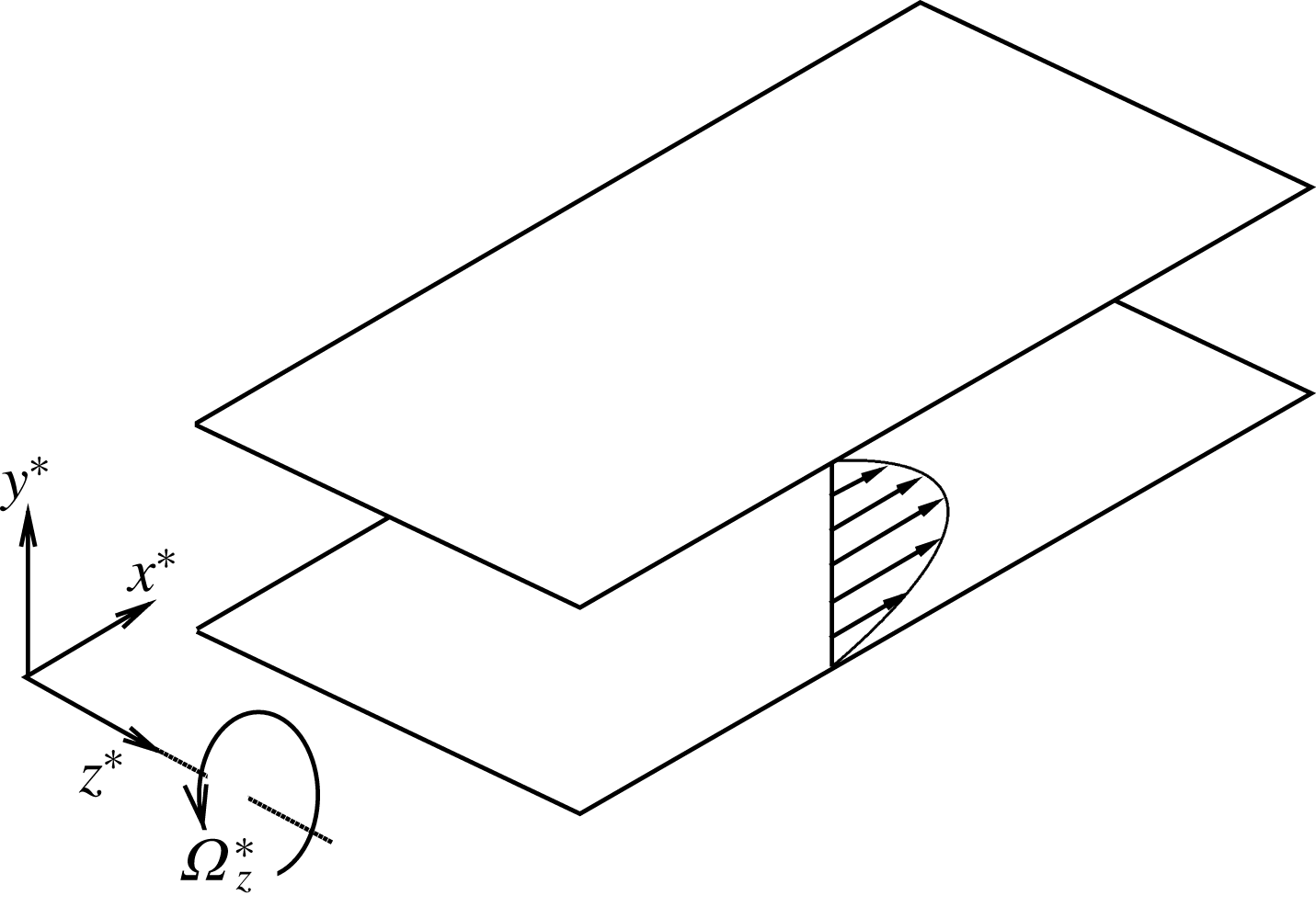
Sketch of the three-dimensional spanwise rotating plane Poiseuille flow.

In the present work, our focus is the 2D/3C model in RPPF and we first would like to present the fully three-dimensional (3-D) RPPF. As sketched in figure 1, the flow is between two stationary parallel and infinite planes which are located at
 $y^{\ast }=0$
and
 $2h^{\ast }$
, respectively, and it is driven by a constant mean pressure gradient
 $-\text{d}P^{\ast }/\text{d}x^{\ast }$
. The whole system rotates in the spanwise direction with a constant angular velocity
 $\unicode[STIX]{x1D6FA}_{z}^{\ast }$
. The bulk mean velocity is defined as
 $U_{b}^{\ast }=\int _{0}^{2h^{\ast }}u^{\ast }\,\text{d}y^{\ast }/2h^{\ast }$
, where
 $h^{\ast }$
is the channel half-width and
 $\unicode[STIX]{x1D708}^{\ast }$
is the kinematic viscosity. In the following,
 $^{\ast }$
denotes a dimensional quantity unless otherwise stated,
 $(x_{1},x_{2},x_{3})$
or
 $(x,y,z)$
denote coordinates in the streamwise, wall-normal and spanwise directions, respectively, and
 $(u_{1},u_{2},u_{3})$
or
 $(u,v,w)$
are the corresponding velocity components. With the velocity and length scales
 $U_{b}^{\ast }$
and
 $h^{\ast }$
, the Reynolds number and rotation number can be defined as
 $Re={U_{b}}^{\ast }h^{\ast }/\unicode[STIX]{x1D708}^{\ast }$
and
 $Ro=2\unicode[STIX]{x1D6FA}_{z}^{\ast }h^{\ast }/{U_{b}}^{\ast }$
respectively, and the non-dimensionalized governing equations are as follows:
 $$\begin{eqnarray}\left.\begin{array}{@{}c@{}}\unicode[STIX]{x1D735}\boldsymbol{\cdot }\boldsymbol{u}=0,\\ \displaystyle \frac{\unicode[STIX]{x2202}\boldsymbol{u}}{\unicode[STIX]{x2202}t}+\boldsymbol{u}\boldsymbol{\cdot }\unicode[STIX]{x1D735}\boldsymbol{u}=-\unicode[STIX]{x1D735}p+Re^{-1}\unicode[STIX]{x0394}\boldsymbol{u}-Ro\boldsymbol{e}_{z}\times \boldsymbol{u},\end{array}\right\}\end{eqnarray}$$
where the constant fluid density
 $\unicode[STIX]{x1D70C}$
is dropped for convenience and the centrifugal force is absorbed into the pressure.
2.1 The 2D/3C model in RPPF
Recently, the 2D/3C model was proposed to obtain a simplified model which is nonlinear and analytically tractable. In the 2D/3C model, all quantities except the driving mean pressure gradient in RPPF are assumed to be uniform in the streamwise direction (
 $\unicode[STIX]{x2202}/\unicode[STIX]{x2202}x=0$
). It can be derived from the Navier–Stokes equations by performing streamwise averaging while neglecting the fluctuating effect relative to the streamwise-averaged field. The governing equations for the 2D/3C model in RPPF are as follows:
 $$\begin{eqnarray}\left.\begin{array}{@{}c@{}}\displaystyle \frac{\unicode[STIX]{x2202}v}{\unicode[STIX]{x2202}y}+\frac{\unicode[STIX]{x2202}w}{\unicode[STIX]{x2202}z}=0,\\ \displaystyle \frac{\unicode[STIX]{x2202}u}{\unicode[STIX]{x2202}t}+v\frac{\unicode[STIX]{x2202}u}{\unicode[STIX]{x2202}y}+w\frac{\unicode[STIX]{x2202}u}{\unicode[STIX]{x2202}z}=-\frac{\text{d}P}{\text{d}x}+\frac{1}{Re}\left(\frac{\unicode[STIX]{x2202}^{2}u}{\unicode[STIX]{x2202}y^{2}}+\frac{\unicode[STIX]{x2202}^{2}u}{\unicode[STIX]{x2202}z^{2}}\right)+Ro\cdot v,\\ \displaystyle \frac{\unicode[STIX]{x2202}v}{\unicode[STIX]{x2202}t}+v\frac{\unicode[STIX]{x2202}v}{\unicode[STIX]{x2202}y}+w\frac{\unicode[STIX]{x2202}v}{\unicode[STIX]{x2202}z}=-\frac{\unicode[STIX]{x2202}p}{\unicode[STIX]{x2202}y}+\frac{1}{Re}\left(\frac{\unicode[STIX]{x2202}^{2}v}{\unicode[STIX]{x2202}y^{2}}+\frac{\unicode[STIX]{x2202}^{2}v}{\unicode[STIX]{x2202}z^{2}}\right)-Ro\cdot u,\\ \displaystyle \frac{\unicode[STIX]{x2202}w}{\unicode[STIX]{x2202}t}+v\frac{\unicode[STIX]{x2202}w}{\unicode[STIX]{x2202}y}+w\frac{\unicode[STIX]{x2202}w}{\unicode[STIX]{x2202}z}=-\frac{\unicode[STIX]{x2202}p}{\unicode[STIX]{x2202}z}+\frac{1}{Re}\left(\frac{\unicode[STIX]{x2202}^{2}w}{\unicode[STIX]{x2202}y^{2}}+\frac{\unicode[STIX]{x2202}^{2}w}{\unicode[STIX]{x2202}z^{2}}\right).\end{array}\right\}\end{eqnarray}$$
2.2 Thermal analogy
Thermal convection is a classical problem in fluid dynamics and has been studied a lot in the past (Palm Reference Palm1975; Bodenschatz, Pesch & Ahlers Reference Bodenschatz, Pesch and Ahlers2000; Ahlers, Grossmann & Lohse Reference Ahlers, Grossmann and Lohse2009; Lohse & Xia Reference Lohse and Xia2010). In this subsection, the analogy between the 2D/3C RPPF and a special thermal convection will be derived based on a similar approach by Tanaka et al. (Reference Tanaka, Kida, Yanase and Kawahara2000). Introducing new variables
 $\hat{\unicode[STIX]{x1D703}}=-u+Ro\cdot y$
,
 $\hat{v}=v$
,
 ${\hat{w}}=w$
and
 $\hat{p}=p+Ro^{2}y^{2}/2$
and new parameters
 $\hat{\unicode[STIX]{x1D6FC}}=\hat{\unicode[STIX]{x1D708}}=1/Re$
,
 $\hat{q}=-\text{d}P/\text{d}x$
,
 ${\hat{g}}\hat{\unicode[STIX]{x1D6FD}}=Ro$
, equation (2.2) can be rewritten as
 $$\begin{eqnarray}\left.\begin{array}{@{}c@{}}\displaystyle \frac{\unicode[STIX]{x2202}\hat{v}}{\unicode[STIX]{x2202}y}+\frac{\unicode[STIX]{x2202}{\hat{w}}}{\unicode[STIX]{x2202}z}=0,\\ \displaystyle \frac{\unicode[STIX]{x2202}\hat{\unicode[STIX]{x1D703}}}{\unicode[STIX]{x2202}t}+\hat{v}\frac{\unicode[STIX]{x2202}\hat{\unicode[STIX]{x1D703}}}{\unicode[STIX]{x2202}y}+{\hat{w}}\frac{\unicode[STIX]{x2202}\hat{\unicode[STIX]{x1D703}}}{\unicode[STIX]{x2202}z}=-\hat{q}+\hat{\unicode[STIX]{x1D6FC}}\left(\frac{\unicode[STIX]{x2202}^{2}\hat{\unicode[STIX]{x1D703}}}{\unicode[STIX]{x2202}y^{2}}+\frac{\unicode[STIX]{x2202}^{2}\hat{\unicode[STIX]{x1D703}}}{\unicode[STIX]{x2202}z^{2}}\right),\\ \displaystyle \frac{\unicode[STIX]{x2202}\hat{v}}{\unicode[STIX]{x2202}t}+\hat{v}\frac{\unicode[STIX]{x2202}\hat{v}}{\unicode[STIX]{x2202}y}+{\hat{w}}\frac{\unicode[STIX]{x2202}\hat{v}}{\unicode[STIX]{x2202}z}=-\frac{\unicode[STIX]{x2202}\hat{p}}{\unicode[STIX]{x2202}y}+\hat{\unicode[STIX]{x1D708}}\left(\frac{\unicode[STIX]{x2202}^{2}\hat{v}}{\unicode[STIX]{x2202}y^{2}}+\frac{\unicode[STIX]{x2202}^{2}\hat{v}}{\unicode[STIX]{x2202}z^{2}}\right)+{\hat{g}}\hat{\unicode[STIX]{x1D6FD}}\cdot \hat{\unicode[STIX]{x1D703}},\\ \displaystyle \frac{\unicode[STIX]{x2202}{\hat{w}}}{\unicode[STIX]{x2202}t}+\hat{v}\frac{\unicode[STIX]{x2202}{\hat{w}}}{\unicode[STIX]{x2202}y}+{\hat{w}}\frac{\unicode[STIX]{x2202}{\hat{w}}}{\unicode[STIX]{x2202}z}=-\frac{\unicode[STIX]{x2202}\hat{p}}{\unicode[STIX]{x2202}z}+\hat{\unicode[STIX]{x1D708}}\left(\frac{\unicode[STIX]{x2202}^{2}{\hat{w}}}{\unicode[STIX]{x2202}y^{2}}+\frac{\unicode[STIX]{x2202}^{2}{\hat{w}}}{\unicode[STIX]{x2202}z^{2}}\right).\end{array}\right\}\end{eqnarray}$$
Correspondingly, the boundary conditions are changed to
 $\hat{v}={\hat{w}}=0$
at
 $y=0,2$
and
 $\hat{\unicode[STIX]{x1D703}}(0)=0,\hat{\unicode[STIX]{x1D703}}(2)=2Ro$
, and the above thermal analogy is exact mathematically. If we take
 $\hat{\unicode[STIX]{x1D703}}$
as the temperature, the above equations (2.3) can be used to describe a special thermal convection, where the temperature at the upper wall is higher than that at the lower wall and a heat sink exists. Also, it should be noted that the Prandtl number
 $Pr=\hat{\unicode[STIX]{x1D708}}/\hat{\unicode[STIX]{x1D6FC}}\equiv 1$
. In the following, the new variable
 $\hat{\unicode[STIX]{x1D703}}$
will be called ‘temperature’ for simplicity where the thermal analogy is used.
3 Instability of roll cells
In this section, we will study the stability of roll cells in RPPF by virtue of the thermal analogy described above. In the past, the stability of roll cells was studied by Speziale & Thangam (Reference Speziale and Thangam1983), who solved the 2D/3C model in a finite-aspect-ratio channel by an explicit finite-difference approach. Several numerical stability-boundary points were obtained for the onset of roll cell instability in the
 $Re_{c}-Ro$
plot. In the present work, we will show that the linear stability boundary can be analytically determined by a newly defined Rayleigh number,
 $Ra$
, with the help of the thermal analogy. The problem is confined to the point of laminar instability and the driving pressure gradient becomes
 $-\text{d}P/\text{d}x=3/Re$
. In this situation, the basic laminar flow is
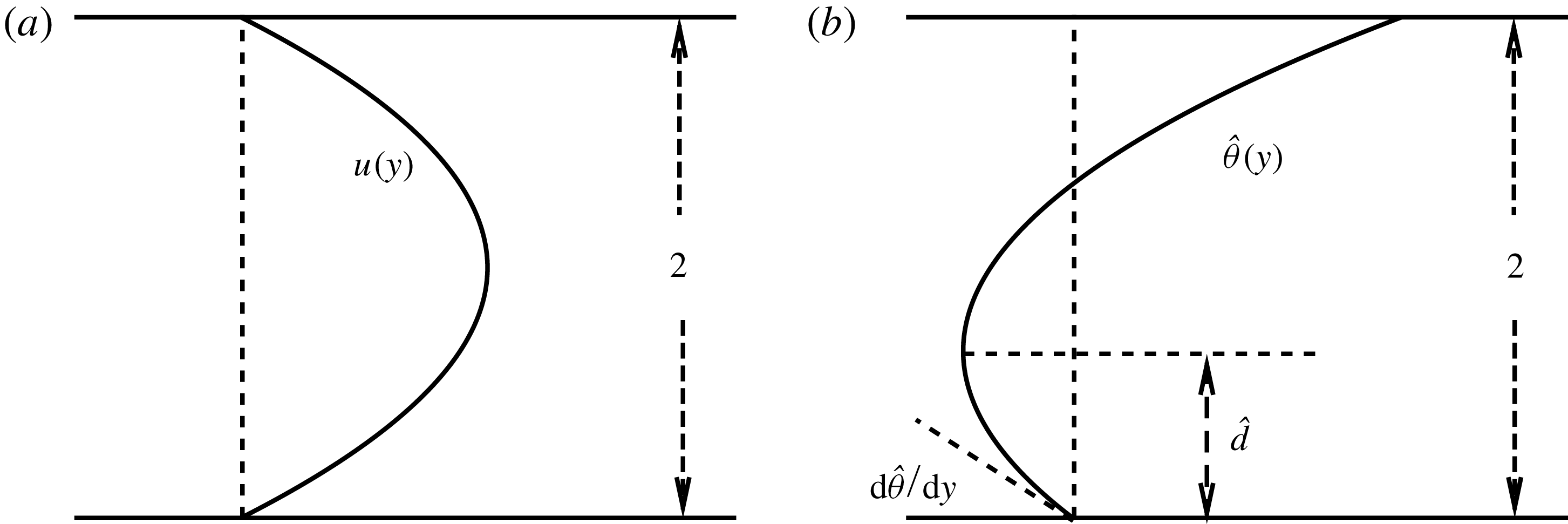
 $u(y)=3y(2-y)/2$
, as shown in figure 2(a).
3.1 Rescaling
With
 $-\text{d}P/\text{d}x=3/Re$
, the corresponding static distribution of
 $\hat{\unicode[STIX]{x1D703}}(y)$
, where
 $\hat{v}={\hat{w}}=0$
, and
 $\unicode[STIX]{x2202}\hat{\unicode[STIX]{x1D703}}/\unicode[STIX]{x2202}t=\unicode[STIX]{x2202}^{2}\hat{\unicode[STIX]{x1D703}}/\unicode[STIX]{x2202}z^{2}=0$
, is
 $\hat{\unicode[STIX]{x1D703}}=Ro\cdot y-3y(2-y)/2$
, as depicted in figure 2(b). It is seen that there is a small region
 $0\leqslant y\leqslant \hat{d}=1-Ro/3$
where the temperature gradient
 $\text{d}\hat{\unicode[STIX]{x1D703}}/\text{d}y<0$
for
 $0<Ro<3$
, although the lower wall is cooler than the upper one. This temperature gradient reaches its maximum absolute value
 $|\hat{\unicode[STIX]{x1D703}}^{\prime }|=3-Ro$
at the lower wall. According to the general inviscid stability criterion in thermal convection, this region with negative temperature gradient is unstable.
In order to focus on the flow and temperature behaviour in this unstable region, a rescaling with characteristic scales
 $\hat{d}$
,
 $\unicode[STIX]{x0394}\unicode[STIX]{x1D703}=\hat{d}\cdot |\hat{\unicode[STIX]{x1D703}}^{\prime }|$
,
 $U=\hat{\unicode[STIX]{x1D6FC}}/\hat{d}$
and
 $T=\hat{d}/U$
, is introduced as
 $$\begin{eqnarray}\displaystyle \tilde{x}_{i}=\frac{x_{i}}{\hat{d}},\quad \tilde{\unicode[STIX]{x1D703}}=\frac{\hat{\unicode[STIX]{x1D703}}}{\unicode[STIX]{x0394}\unicode[STIX]{x1D703}},\quad \tilde{v}=\frac{\hat{v}}{U},\quad \tilde{w}=\frac{{\hat{w}}}{U},\quad \tilde{t}=\frac{t}{T},\quad \tilde{p}=\frac{\hat{p}}{U^{2}} & & \displaystyle\end{eqnarray}$$
and the above equation (2.3) can be reformed as
 $$\begin{eqnarray}\left.\begin{array}{@{}c@{}}\displaystyle \frac{\unicode[STIX]{x2202}\tilde{v}}{\unicode[STIX]{x2202}{\tilde{y}}}+\frac{\unicode[STIX]{x2202}\tilde{w}}{\unicode[STIX]{x2202}\tilde{z}}=0,\\ \displaystyle \frac{\unicode[STIX]{x2202}\tilde{\unicode[STIX]{x1D703}}}{\unicode[STIX]{x2202}\tilde{t}}+\tilde{v}\frac{\unicode[STIX]{x2202}\tilde{\unicode[STIX]{x1D703}}}{\unicode[STIX]{x2202}{\tilde{y}}}+\tilde{w}\frac{\unicode[STIX]{x2202}\tilde{\unicode[STIX]{x1D703}}}{\unicode[STIX]{x2202}\tilde{z}}=-\tilde{q}+\left(\frac{\unicode[STIX]{x2202}^{2}\tilde{\unicode[STIX]{x1D703}}}{\unicode[STIX]{x2202}{\tilde{y}}^{2}}+\frac{\unicode[STIX]{x2202}^{2}\tilde{\unicode[STIX]{x1D703}}}{\unicode[STIX]{x2202}\tilde{z}^{2}}\right),\\ \displaystyle \frac{\unicode[STIX]{x2202}\tilde{v}}{\unicode[STIX]{x2202}\tilde{t}}+\tilde{v}\frac{\unicode[STIX]{x2202}\tilde{v}}{\unicode[STIX]{x2202}{\tilde{y}}}+\tilde{w}\frac{\unicode[STIX]{x2202}\tilde{v}}{\unicode[STIX]{x2202}\tilde{z}}=-\frac{\unicode[STIX]{x2202}\tilde{p}}{\unicode[STIX]{x2202}{\tilde{y}}}+Pr\left(\frac{\unicode[STIX]{x2202}^{2}\tilde{v}}{\unicode[STIX]{x2202}{\tilde{y}}^{2}}+\frac{\unicode[STIX]{x2202}^{2}\tilde{v}}{\unicode[STIX]{x2202}\tilde{z}^{2}}\right)+RaPr\tilde{\unicode[STIX]{x1D703}},\\ \displaystyle \frac{\unicode[STIX]{x2202}\tilde{w}}{\unicode[STIX]{x2202}\tilde{t}}+\tilde{v}\frac{\unicode[STIX]{x2202}\tilde{w}}{\unicode[STIX]{x2202}{\tilde{y}}}+\tilde{w}\frac{\unicode[STIX]{x2202}\tilde{w}}{\unicode[STIX]{x2202}\tilde{z}}=-\frac{\unicode[STIX]{x2202}\tilde{p}}{\unicode[STIX]{x2202}\tilde{z}}+Pr\left(\frac{\unicode[STIX]{x2202}^{2}\tilde{w}}{\unicode[STIX]{x2202}{\tilde{y}}^{2}}+\frac{\unicode[STIX]{x2202}^{2}\tilde{w}}{\unicode[STIX]{x2202}\tilde{z}^{2}}\right),\end{array}\right\}\end{eqnarray}$$
with
 $\tilde{q}=1$
and
 $Pr=1$
.
 $Ra={\hat{g}}\hat{\unicode[STIX]{x1D6FD}}\unicode[STIX]{x0394}\unicode[STIX]{x1D703}\hat{d}/(U^{2}Pr)={\hat{g}}\hat{\unicode[STIX]{x1D6FD}}|\hat{\unicode[STIX]{x1D703}}^{\prime }|\hat{d}^{4}/\hat{\unicode[STIX]{x1D708}}\hat{\unicode[STIX]{x1D6FC}}=Re^{2}Ro(3-Ro)^{5}/81$
is a newly defined Rayleigh number. The channel height will be changed to
 $H=2/\hat{d}=6/(3-Ro)$
and the boundary conditions are changed to
 $$\begin{eqnarray}\displaystyle \tilde{v}=\tilde{w}=0\quad \text{at }{\tilde{y}}=0,H,\quad \text{and}\quad \tilde{\unicode[STIX]{x1D703}}(0)=0,\tilde{\unicode[STIX]{x1D703}}(H)=6Ro/(3-Ro)^{2}. & & \displaystyle\end{eqnarray}$$
With the rescaling, the height of the inviscid unstable region changes to 1 and the temperature gradient becomes
 ${\tilde{y}}-1$
. It can be seen that the above thermal analogy and rescaling then map the two parameters
 $Re$
and
 $Ro$
in a 2D/3C RPPF to the Rayleigh number
 $Ra$
and a geometric parameter
 $H$
in the special thermal convection problem.
(a) Profile of laminar velocity
 $u(y)=3y(2-y)/2$
in the 2D/3C model described by (2.2) with
 $-\text{d}P/\text{d}x=3/Re$
; (b) the corresponding distribution of
 $\hat{\unicode[STIX]{x1D703}}(y)=-u+Ro\cdot y$
. Here,
 $\hat{d}=1-Ro/3$
is the location where
 $\hat{\unicode[STIX]{x1D703}}$
reaches its minimum value and
 $\text{d}\hat{\unicode[STIX]{x1D703}}/\text{d}y=Ro-3$
is the gradient in the wall-normal direction at the bottom wall.

3.2 Linear stability analysis
In this section, the linear stability analysis will be discussed by following the conventional procedure, where the instantaneous flow variables are separated into the basic flow and some infinitesimal disturbances. With the disturbance variables inheriting the symbols of the original instantaneous ones in (2.2) and (3.2), the corresponding linearized disturbance equations will lead to the following forms by neglecting the products of the disturbances:
 $$\begin{eqnarray}\left.\begin{array}{@{}c@{}}\displaystyle \frac{\unicode[STIX]{x2202}v}{\unicode[STIX]{x2202}y}+\frac{\unicode[STIX]{x2202}w}{\unicode[STIX]{x2202}z}=0,\\ \displaystyle \frac{\unicode[STIX]{x2202}u}{\unicode[STIX]{x2202}t}=\frac{1}{Re}\left(\frac{\unicode[STIX]{x2202}^{2}u}{\unicode[STIX]{x2202}y^{2}}+\frac{\unicode[STIX]{x2202}^{2}u}{\unicode[STIX]{x2202}z^{2}}\right)-(3-3y-Ro)v,\\ \displaystyle \frac{\unicode[STIX]{x2202}v}{\unicode[STIX]{x2202}t}=-\frac{\unicode[STIX]{x2202}p}{\unicode[STIX]{x2202}y}+\frac{1}{Re}\left(\frac{\unicode[STIX]{x2202}^{2}v}{\unicode[STIX]{x2202}y^{2}}+\frac{\unicode[STIX]{x2202}^{2}v}{\unicode[STIX]{x2202}z^{2}}\right)-Ro\cdot u,\\ \displaystyle \frac{\unicode[STIX]{x2202}w}{\unicode[STIX]{x2202}t}=-\frac{\unicode[STIX]{x2202}p}{\unicode[STIX]{x2202}z}+\frac{1}{Re}\left(\frac{\unicode[STIX]{x2202}^{2}w}{\unicode[STIX]{x2202}y^{2}}+\frac{\unicode[STIX]{x2202}^{2}w}{\unicode[STIX]{x2202}z^{2}}\right)\end{array}\right\}\end{eqnarray}$$
and
 $$\begin{eqnarray}\left.\begin{array}{@{}c@{}}\displaystyle \frac{\unicode[STIX]{x2202}\tilde{v}}{\unicode[STIX]{x2202}{\tilde{y}}}+\frac{\unicode[STIX]{x2202}\tilde{w}}{\unicode[STIX]{x2202}\tilde{z}}=0,\\ \displaystyle \frac{\unicode[STIX]{x2202}\tilde{\unicode[STIX]{x1D703}}}{\unicode[STIX]{x2202}\tilde{t}}=\left(\frac{\unicode[STIX]{x2202}^{2}\tilde{\unicode[STIX]{x1D703}}}{\unicode[STIX]{x2202}{\tilde{y}}^{2}}+\frac{\unicode[STIX]{x2202}^{2}\tilde{\unicode[STIX]{x1D703}}}{\unicode[STIX]{x2202}\tilde{z}^{2}}\right)-({\tilde{y}}-1)\tilde{v},\\ \displaystyle \frac{\unicode[STIX]{x2202}\tilde{v}}{\unicode[STIX]{x2202}\tilde{t}}=-\frac{\unicode[STIX]{x2202}\tilde{p}}{\unicode[STIX]{x2202}{\tilde{y}}}+Pr\left(\frac{\unicode[STIX]{x2202}^{2}\tilde{v}}{\unicode[STIX]{x2202}{\tilde{y}}^{2}}+\frac{\unicode[STIX]{x2202}^{2}\tilde{v}}{\unicode[STIX]{x2202}\tilde{z}^{2}}\right)+RaPr\tilde{\unicode[STIX]{x1D703}},\\ \displaystyle \frac{\unicode[STIX]{x2202}\tilde{w}}{\unicode[STIX]{x2202}\tilde{t}}=-\frac{\unicode[STIX]{x2202}\tilde{p}}{\unicode[STIX]{x2202}\tilde{z}}+Pr\left(\frac{\unicode[STIX]{x2202}^{2}\tilde{w}}{\unicode[STIX]{x2202}{\tilde{y}}^{2}}+\frac{\unicode[STIX]{x2202}^{2}\tilde{w}}{\unicode[STIX]{x2202}\tilde{z}^{2}}\right),\end{array}\right\}\end{eqnarray}$$
and the boundary conditions become
 $u=v=w=0$
at
 $y=0,2$
and
 $\tilde{v}=\tilde{w}=\tilde{\unicode[STIX]{x1D703}}=0$
at
 ${\tilde{y}}=0,H$
respectively.
Following the conventional procedure, the normal-mode description of the disturbance for (3.4) is considered and it is given by
 $$\begin{eqnarray}[u,v,w,p]={\textstyle \frac{1}{2}}\{[-\text{i}U(y),-\text{i}V(y),W(y),-\text{i}P(y)]\text{e}^{\unicode[STIX]{x1D70E}t+\text{i}az}+\text{complex conjugate}\}.\end{eqnarray}$$
Here,
 $U(y),V(y),W(y)$
and
 $P(y)$
are eigenfunctions of the disturbance field, and
 $\unicode[STIX]{x1D70E}$
is the inverse time constant of the spanwise mode
 $a$
. Substitution of (3.6) into (3.4) will lead to a set of ordinary differential equations for the streamwise and transverse disturbance velocities. In the present study, we limit our interest to the neutral stability with
 $\unicode[STIX]{x1D70E}=0$
, and the simplified governing equation becomes
 $$\begin{eqnarray}\left.\begin{array}{@{}c@{}}(D^{2}-a^{2})^{3}V=-a^{2}Re^{2}Ro(3-Ro-3y)V,\\ V=DV=(D^{4}-2a^{2}D^{2})V=0\quad \text{at }y=0,2,\end{array}\right\}\end{eqnarray}$$
with
 $D\equiv \unicode[STIX]{x2202}/\unicode[STIX]{x2202}y$
.
Similarly, the normal-mode description of the disturbance for (3.5) can also be introduced
 $$\begin{eqnarray}[\tilde{\unicode[STIX]{x1D703}},\tilde{v},\tilde{w},\tilde{p}]={\textstyle \frac{1}{2}}\{[-\text{i}\tilde{\unicode[STIX]{x1D6E9}}({\tilde{y}}),-\text{i}\tilde{V}({\tilde{y}}),\tilde{W}({\tilde{y}}),-\text{i}\tilde{P}({\tilde{y}})]\text{e}^{\tilde{\unicode[STIX]{x1D70E}}\tilde{t}+\text{i}\tilde{a}\tilde{z}}+\text{complex conjugate}\}.\end{eqnarray}$$
With
 $\tilde{D}=\unicode[STIX]{x2202}/\unicode[STIX]{x2202}{\tilde{y}}$
, the simplified governing equation related to (3.5) becomes
 $$\begin{eqnarray}\left.\begin{array}{@{}c@{}}(\tilde{D}^{2}-\tilde{a}^{2})^{3}\tilde{V}=-\tilde{a}^{2}Ra(1-{\tilde{y}})\tilde{V},\\ \tilde{V}=\tilde{D}\tilde{V}=(\tilde{D}^{4}-2\tilde{a}^{2}\tilde{D}^{2})\tilde{V}=0\quad \text{at }{\tilde{y}}=0,H.\end{array}\right\}\end{eqnarray}$$
It is easy to verify that the two equations (3.7) and (3.9) are equivalent, and that if
 $V(y)$
satisfies (3.7), then
 $\tilde{V}({\tilde{y}})=V(2{\tilde{y}}/H)$
satisfies (3.9) with parameters
 $Ra=Re^{2}Ro(3-Ro)^{5}/81$
,
 $H=6/(3-Ro)$
and
 $\tilde{a}=(3-Ro)a/3$
. Thus, solving (3.7) is sufficient for the analysis. In the present work, a Chebyshev collocation spectral method is used to solve (3.7) and to obtain eigensolution
 $V(y)$
. If
 $V(y)$
is obtained, being a real function with maximum value 1 and
 $\text{d}^{2}V/\text{d}y^{2}|_{y=0}>0$
, the related normal modes of
 $v,w,u$
for (3.4) can be derived as
 $$\begin{eqnarray}\left.\begin{array}{@{}c@{}}v=V(y)\sin (az),\\ w=W(y)\cos (az)=DV\cos (az)/a,\\ u=U(y)\sin (az)=-(D^{2}-a^{2})^{2}V\sin (az)/a^{2}ReRo.\end{array}\right\}\end{eqnarray}$$
With transformation, the related normal modes of
 $\tilde{w},\tilde{\unicode[STIX]{x1D703}}$
for (3.5) are
 $$\begin{eqnarray}\left.\begin{array}{@{}c@{}}\tilde{w}=\tilde{W}({\tilde{y}})\cos (\tilde{a}\tilde{z})=w(2{\tilde{y}}/H,2\tilde{z}/H),\\ \tilde{\unicode[STIX]{x1D703}}=\tilde{\unicode[STIX]{x1D6E9}}({\tilde{y}})\sin (\tilde{a}\tilde{z})=-9u(2{\tilde{y}}/H,2\tilde{z}/H)/Re(3-Ro)^{3}.\end{array}\right\}\end{eqnarray}$$
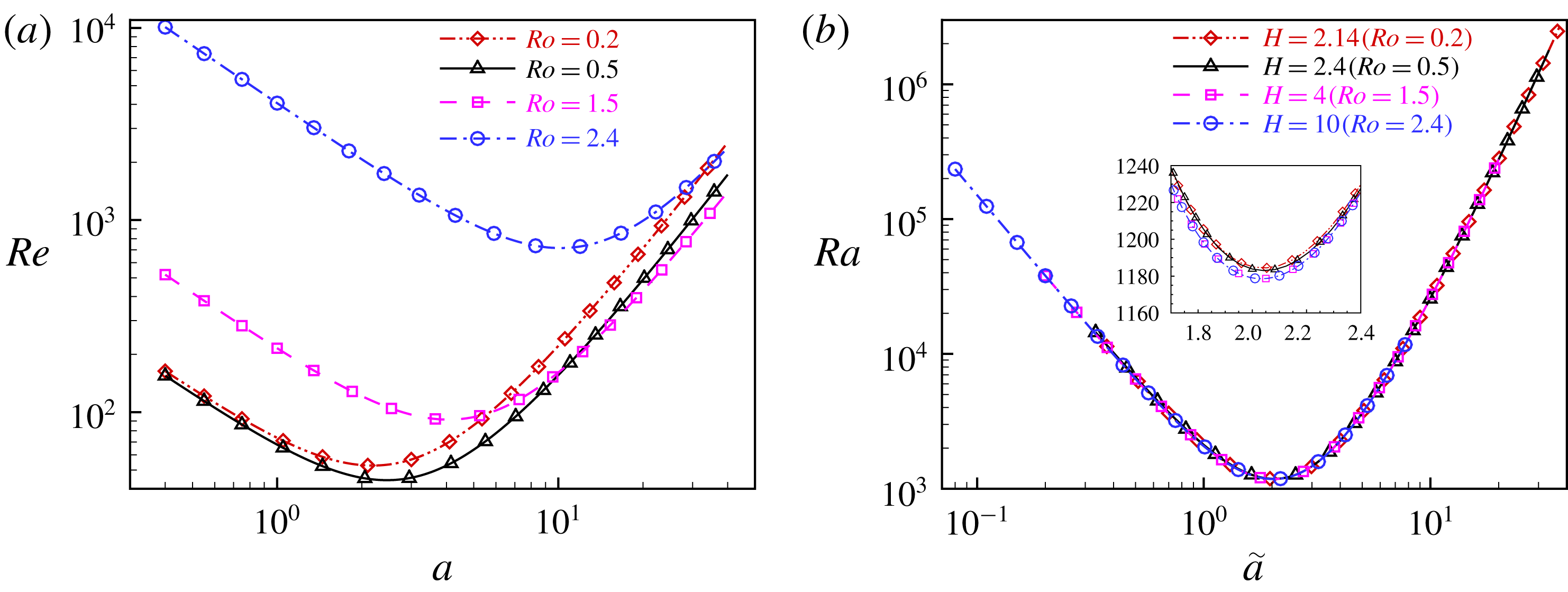
In figure 3(a), we show the neutrally stable solutions of (3.7) at
 $Ro=0.2,0.5,1.5$
and 2.4 from our numerical results. It is seen that
 $Re$
first decreases with
 $a$
and then increases with it at a fixed
 $Ro$
. A critical point
 $(a_{c}(Ro),Re_{c}(Ro))$
can be discerned on the neutral stability curve
 $Re(a;Ro)$
at any fixed
 $Ro$
. For
 $Ro\geqslant 0.5$
, both
 $a_{c}(Ro)$
and
 $Re_{c}(Ro)$
increase with
 $Ro$
. This trend is consistent with the previous result in Lezius & Johnston (Reference Lezius and Johnston1976), where they could only numerically solve their equations with
 $Ro\leqslant 1.75$
due to their numerical method. Correspondingly, the parameter-transformed neutral stability curves of
 $Ra(\tilde{a};H(Ro))$
at different
 $H(Ro)$
are shown in figure 3(b). It is surprising to see that the curves almost collapse on top of each other, and very mild deviations can be discerned only by local amplification. Therefore, it is reasonable to conjecture that the neutral stability curves of 2D/3C RPPFs are basically the same at different
 $Ro$
and we may predict the curves at different
 $Ro$
by using the information at a certain
 $Ro$
and back-and-forth transformations between
 $(a(Ro),Re(Ro))$
and
 $(\tilde{a}(H(Ro)),Ra(H(Ro)))$
.
Neutral stability curves (a)
 $Re(a;Ro)$
for 2D/3C RPPF at
 $Ro=0.2,0.5,1.5$
and 2.4; (b) the corresponding curves
 $Ra(\tilde{a};H(Ro))$
for the thermal convection. Inset shows the enlarged region around
 $\tilde{a}=2$
.

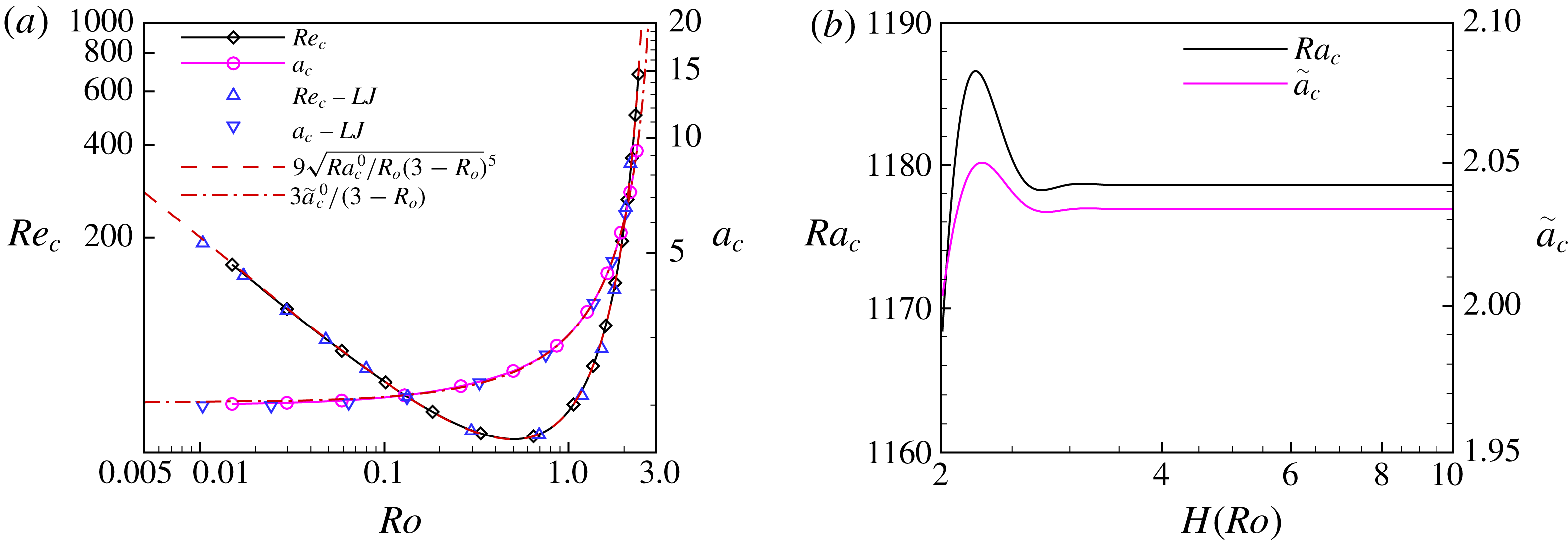
(a) Critical Reynolds number
 $Re_{c}$
and critical wavenumber
 $a_{c}$
for the neutral stability curve at different
 $Ro$
. Solid lines with diamonds and circles are
 $Re_{c}$
and
 $a_{c}$
obtained from computation;
 ${\vartriangle}$
and
 $\triangledown$
are
 $Re_{c}$
and
 $a_{c}$
from Lezius & Johnston (Reference Lezius and Johnston1976); dashed line and dash-dotted line are the analytic approximations
 $Re_{c}=9\sqrt{Ra_{c}^{0}/Ro(3-Ro)^{5}}$
and
 $a_{c}=3\tilde{a}_{c}^{0}/(3-Ro)$
with
 $Ra_{c}^{0}=1178.6,\tilde{a}_{c}^{0}=2.034$
, respectively. (b) Calculated
 $Ra_{c}$
and
 $\tilde{a}_{c}$
with different
 $H(Ro)$
.

In order to further understand the instability of roll cells, we display in figure 4(a) the critical Reynolds number
 $Re_{c}$
and critical wavenumber (or cell frequency)
 $a_{c}$
for the neutral stability curve at different
 $Ro$
. The previous calculated results from Lezius & Johnston (Reference Lezius and Johnston1976) are also shown for comparison (the channel height was 1, thus the values have to be re-scaled by a factor of 2). It is evident that our results match very well with those of Lezius & Johnston (Reference Lezius and Johnston1976). The values of
 $Ra_{c}$
and
 $\tilde{a}_{c}$
related to the corresponding thermal convection at different
 $H(Ro)$
are depicted in figure 4(b). It is interesting to see that both
 $Ra_{c}$
and
 $\tilde{a}_{c}$
vary very slightly if
 $H\gtrsim 2.6$
(
 $Ro\approx 0.7$
) and they are almost constant when
 $H\gtrsim 3.5$
(
 $Ro\approx 1.29$
). The values are
 $Ra_{c}^{0}=1178.6,\tilde{a}_{c}^{0}=2.034$
. The maximum and minimum values of
 $Ra_{c}$
are 1186.61 and 1168.37, which are approximately 0.68 % and
 $-0.87\,\%$
as compared to
 $Ra_{c}^{0}$
. For
 $\tilde{a}_{c}$
, the peak values are 2.05 and 2.0034, and the discrepancies are 0.78 % and
 $-1.5\,\%$
, which are quite small. With the assumption that
 $Ra_{c}\equiv Ra_{c}^{0}$
and
 $\tilde{a}_{c}\equiv \tilde{a}_{c}^{0}$
, analytic expressions for
 $Re_{c}$
and
 $a_{c}$
can be obtained:
 $$\begin{eqnarray}Re_{c}=9\sqrt{\frac{Ra_{c}^{0}}{Ro(3-Ro)^{5}}}\quad \text{and}\quad a_{c}=\frac{3\tilde{a}_{c}^{0}}{3-Ro}.\end{eqnarray}$$
The analytic expressions (3.12) with
 $Ra_{c}^{0}=1178.6,\tilde{a}_{c}^{0}=2.034$
are also shown in figure 4(a), and it is apparent that they match very well with the present computed results and those from Lezius & Johnston (Reference Lezius and Johnston1976) for the whole
 $Ro$
range considered. The lowest
 $Re_{c}\approx 44.22$
can be obtained at
 $Ro=0.5$
, which is very close to the value
 $44.27$
by Lezius & Johnston (Reference Lezius and Johnston1976). Furthermore, the analytic expressions (3.12) give the same asymptotic trends as those reported in Lezius & Johnston (Reference Lezius and Johnston1976) at two limiting cases
 $$\begin{eqnarray}\displaystyle Re_{c}\sim Ro^{-1/2}\quad \text{and}\quad a_{c}\sim \text{constant if }Ro\rightarrow 0. & & \displaystyle\end{eqnarray}$$
 $$\begin{eqnarray}\displaystyle Re_{c}\sim (3-Ro)^{-5/2}\quad \text{and}\quad a_{c}\sim (3-Ro)^{-1}\quad \text{if }Ro\rightarrow 3. & & \displaystyle\end{eqnarray}$$
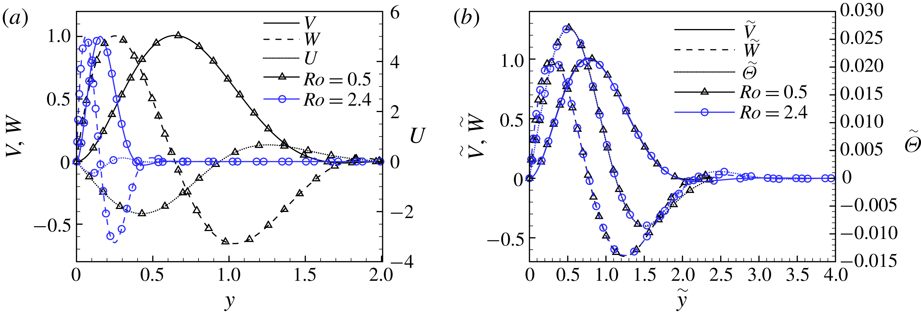
Figure 5(a,b) shows the critical eigensolutions of
 $V(y),W(y),U(y)$
from (3.7) at two different rotation numbers
 $Ro=0.5$
and
 $2.4$
and their corresponding functions of
 $\tilde{V}({\tilde{y}}),\tilde{W}({\tilde{y}}),\tilde{\unicode[STIX]{x1D6E9}}({\tilde{y}})$
from (3.9). It is obvious, from the view of RPPF as shown in figure 5(a), that the critical eigenfunctions shrink towards the lower wall but maintain similar shapes as
 $Ro$
increases. A similar trend was also observed by Lezius & Johnston (Reference Lezius and Johnston1976), who compared their numerical results at
 $Ro=0.5$
and 1.5. However, if we view the problem from the thermal convection viewpoint, as depicted in figure 5(b), the critical eigensolutions again collapse onto each other for
 ${\tilde{y}}\lesssim 1.8$
. The good collapse behaviour demonstrates that the rescaling introduced in the present work based on the thermal analogy and the related control parameters
 $Ra$
and
 $H$
are well chosen.
(a) Critical eigensolutions of
 $V(y),W(y),U(y)$
from (3.7) at
 $Ro=0.5$
(
 $Re_{c}\approx 44.3$
and
 $a_{c}\approx 2.45$
) and 2.4 (
 $Re_{c}\approx 715.2$
and
 $a_{c}\approx 10.15$
); (b) the corresponding functions of
 $\tilde{V}({\tilde{y}}),\tilde{W}({\tilde{y}}),\tilde{\unicode[STIX]{x1D6E9}}({\tilde{y}})$
from (3.9).
 $Ro=0.5$
(
 $Re_{c}\approx 44.3$
and
 $a_{c}\approx 2.45$
) corresponds to
 $H=2.4$
(
 $Ra_{c}\approx 1183.0$
and
 $\tilde{a}_{c}\approx 2.04$
), while
 $Ro=2.4$
(
 $Re_{c}\approx 715.2$
and
 $a_{c}\approx 10.15$
) corresponds to
 $H=10$
(
 $Ra_{c}\approx 1178.6$
and
 $\tilde{a}_{c}\approx 2.034$
).

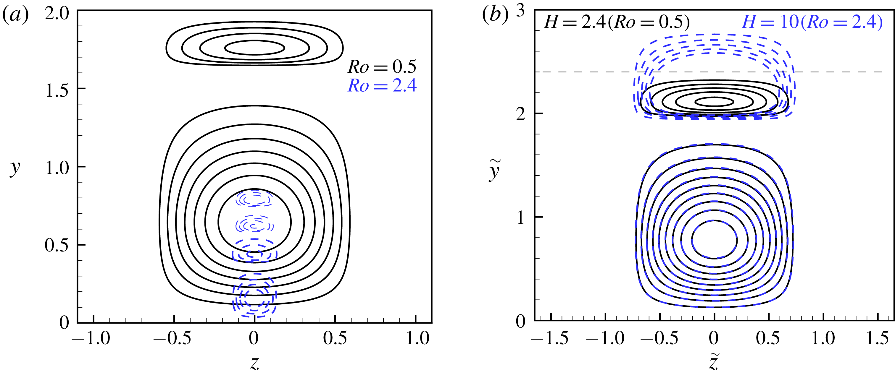
(a) Critical streamfunction at
 $Ro=0.5$
(solid) and 2.4 (dashed). For
 $Ro=0.5$
,
 $\unicode[STIX]{x1D713}=-0.35(0.05)-0.05$
for the bottom roll and
 $\unicode[STIX]{x1D713}=0.001(0.001)0.004$
for the upper one. For
 $Ro=2.4$
, the values of
 $\unicode[STIX]{x1D713}$
are
 $-0.08(0.02)-0.02$
,
 $0.0005(0.001)0.0025$
,
 $-0.00025(0.00005)-0.0001$
and
 $0.00001,0.000015,0.00002$
for the rolls from the bottom to upper wall. (b) Corresponding critical streamfunction calculated from
 $\tilde{v},\tilde{w}$
.
 $\tilde{\unicode[STIX]{x1D713}}=-0.45(0.05)-0.05$
for the bottom roll and
 $\tilde{\unicode[STIX]{x1D713}}=0.001(0.001)0.005$
for the upper one. The dashed line at
 ${\tilde{y}}=2.4$
shows the upper boundary of
 $H=2.4(Ro=0.5)$
. The related values of
 $Re_{c}(Ra_{c})$
and
 $a_{c}(\tilde{a}_{c})$
are the same as those in figure 5.

Figure 6(a) shows the critical streamfunction
 $\unicode[STIX]{x1D713}=-V(y)\cos (az)/a$
obtained from (3.7) at
 $Ro=0.5$
and 2.4. At
 $Ro=0.5$
, two roll cells can be observed. The bottom one is bigger in size and larger in the value of
 $\unicode[STIX]{x1D713}$
. When
 $Ro$
increases to 2.4, the roll cells become smaller in size and their
 $\unicode[STIX]{x1D713}$
values also decrease as compared to the those at
 $Ro=0.5$
. The sizes and
 $\unicode[STIX]{x1D713}$
values of the four roll cells shown in the figure become smaller as their distances from the bottom wall increase. This trend again is similar to that reported by Lezius & Johnston (Reference Lezius and Johnston1976). Nevertheless, the critical streamfunction
 $\tilde{\unicode[STIX]{x1D713}}$
for the corresponding thermal convection problem, as shown in figure 6(b), shows a very good collapse behaviour at two different
 $H(Ro)$
cases for the roll cell near the bottom wall. This is not surprising anymore since we have shown that the critical eigenfunctions again collapse onto each other for
 ${\tilde{y}}\lesssim 1.8$
. The roll cells further away from the wall, however, show obvious differences. This is also consistent with the fact shown in figure 5(b). The collapse of the first roll cell at different
 $H(Ro)$
again verifies the good choice of the rescaling and the related control parameters
 $Ra$
and
 $H$
.
From the above discussion, it is clear that, with the help of a thermal analogy and a rescaling with well-chosen parameters
 $Ra$
and
 $H$
, the instability of roll cells in 2D/3C RPPF at different
 $Ro$
can be simplified and the neutral stability curves, the critical Reynolds number
 $Re_{c}$
, the critical cell frequency
 $a_{c}$
, the critical eigensolutions of
 $V(y),W(y),U(y)$
and the critical streamfunctions at different
 $Ro$
can be obtained if they are known at a certain
 $Ro$
. Nevertheless, as pointed out by one of the anonymous referees, the above analysis is valid in the range of
 $0\leqslant Ro\leqslant 3$
due to the constraint of the characteristic scale
 $\hat{d}=1-Ro/3>0$
. For
 $Ro\geqslant 3$
, the static temperature
 $\hat{\unicode[STIX]{x1D703}}$
increases monotonically with
 $y$
across the channel and the flow is stable following the general inviscid stability criterion. In this situation, the above model and rescaling are not required. Furthermore, past works also showed that turbulence would relaminarize if
 $Ro\geqslant 3$
(Grundestam et al.
Reference Grundestam, Wallin and Johansson2008; Wallin et al.
Reference Wallin, Grundestam and Johansson2013).
4 The case of 2D/3C RPPF in a turbulent state
In the previous section, we have already shown that the 2D/3C model can be used to study the instability of roll cells in RPPF, and the thermal analogy and rescaling can map the two control parameters
 $Re$
and
 $Ro$
in RPPF to a newly defined
 $Ra$
and the channel height
 $H$
in a special 2-D thermal convection problem. In fact, the thermal analogy is not restricted to the laminar state, and it is also valid for turbulent states if the heat sink
 $\hat{q}$
is redefined as
 $-\text{d}P/\text{d}x$
in turbulent states. In this section, numerical simulations of the 2D/3C RPPF will be performed and the turbulence statistics and flow structures will be investigated. Our results show that the 2D/3C RPPF model is self-sustained, and the turbulence can persist without any extra forcing excitation.
4.1 Numerical description
In this section, we will consider the RPPF flows driven by a constant mean pressure gradient
 $-\text{d}P^{\ast }/\text{d}x$
, where the global friction Reynolds number
 $Re_{\unicode[STIX]{x1D70F}}=u_{\unicode[STIX]{x1D70F}}^{\ast }h^{\ast }/\unicode[STIX]{x1D708}^{\ast }$
is fixed at 180. Here,
 $u_{\unicode[STIX]{x1D70F}}^{\ast }=\sqrt{(\unicode[STIX]{x1D70F}_{w;p}^{\ast }+\unicode[STIX]{x1D70F}_{w;s}^{\ast })/2}=\sqrt{-\text{d}P^{\ast }/\text{d}x^{\ast }(h^{\ast }/\unicode[STIX]{x1D70C}^{\ast })}$
is the global friction velocity with
 $\unicode[STIX]{x1D70F}_{w;p}^{\ast }$
and
 $\unicode[STIX]{x1D70F}_{w;s}^{\ast }$
being the friction velocities at the walls of the pressure and suction sides. With
 $u_{\unicode[STIX]{x1D70F}}^{\ast }$
and
 $h^{\ast }$
as the characteristic scales, the governing equation (2.1) keeps its form with substitutions of
 $Re$
and
 $Ro$
by
 $Re_{\unicode[STIX]{x1D70F}}$
and
 $Ro_{\unicode[STIX]{x1D70F}}=2\unicode[STIX]{x1D6FA}_{z}^{\ast }h^{\ast }/u_{\unicode[STIX]{x1D70F}}^{\ast }$
. Similar substitutions can be used in (2.2) while
 $-\text{d}P/\text{d}x=1$
. In the following discussions, all quantities are normalized by
 $u_{\unicode[STIX]{x1D70F}}^{\ast }$
and
 $h^{\ast }$
and the conventional superscript ‘
 $+$
’ is neglected for simplicity.
For fully 3-D RPPF and the 2D/3C RPPF, the equations (2.1) and (2.2) are solved using the same pseudo-spectral method which was used before (Xia et al.
Reference Xia, Shi and Chen2016). The detailed information about the method can be found in Yang & Pullin (Reference Yang and Pullin2011). In order to carry out the present 2D/3C simulations using the fully 3-D code, the simulation was started by setting the modes with
 $k_{x}\neq 0$
in Fourier space to exactly zero specifically. This is equivalent to copying the cross-section field in the streamwise directions in physical space. Since the highly accurate pseudo-spectral code is used, the
 $k_{x}\neq 0$
modes will be zero during the simulations, and the exact length
 $L_{x}$
and grid points
 $N_{x}$
have no influence on the simulation results. It should be mentioned that the streamfunction approach has been used frequently to numerically solve the 2D/3C model in the past (Speziale & Thangam Reference Speziale and Thangam1983; Gayme et al.
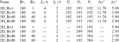
Reference Gayme, McKeon, Papachristodoulou, Bamieh and Doyle2010). Our numerical tests also suggest that a much finer mesh should be used in the spanwise direction. Selected cases from fully 3-D and 2D/3C simulations are listed in table 1.
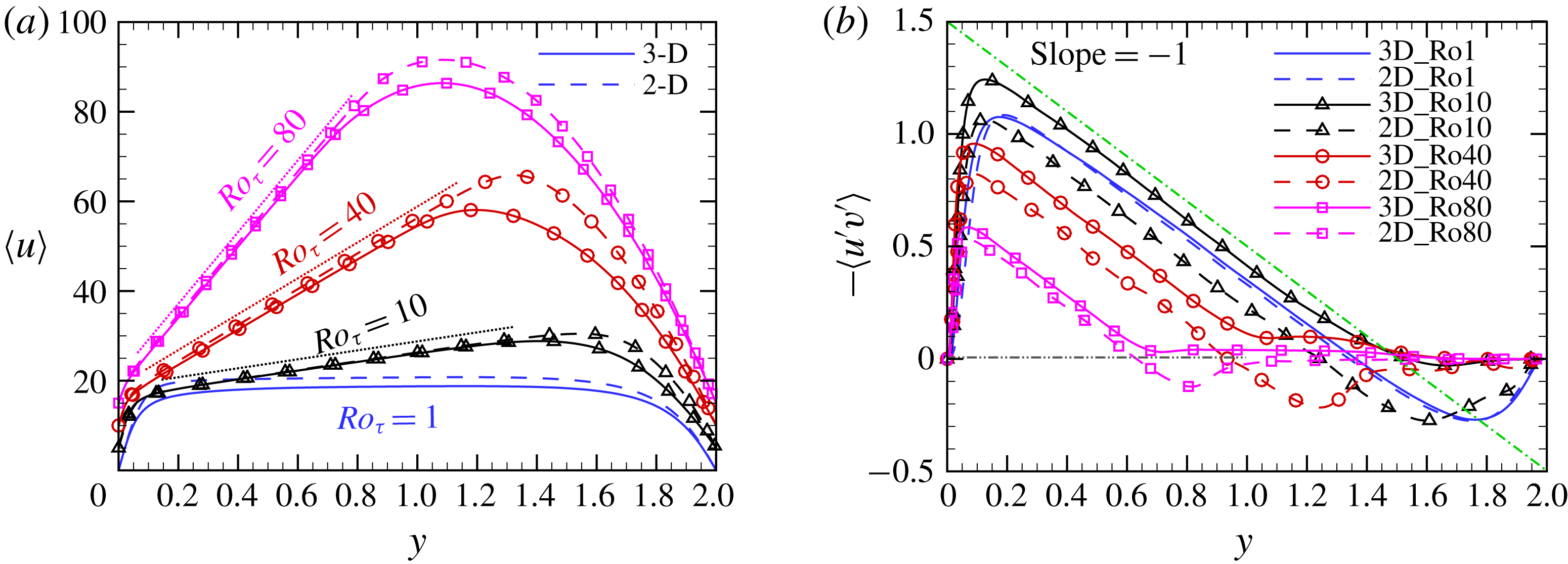
(a) Mean velocity profiles
 $\langle u\rangle$
at different
 $Ro_{\unicode[STIX]{x1D70F}}$
. The solid lines (with/without symbols) are from fully 3-D simulations while the dashed lines (with/without symbols) are from the 2D/3C simulations. The profiles are shifted upward for clarity. (b) Reynolds shear stress
 $-\langle u^{\prime }v^{\prime }\rangle$
from different simulations.

Parameters of 2D/3C and 3-D simulations.

4.2 Statistics and flow structures in 2D/3C RPPFs
In this subsection, the flow statistics will be investigated. In the present study,
 $\langle \unicode[STIX]{x1D719}\rangle$
denotes a quantity that is averaged in the
 $x$
and
 $z$
directions as well as in time
 $t$
for fully 3-D simulations, while it denotes the averaging operator in
 $z$
and
 $t$
for the 2D/3C simulations;
 $\unicode[STIX]{x1D719}^{\prime }\triangleq \unicode[STIX]{x1D719}-\langle \unicode[STIX]{x1D719}\rangle$
denotes the corresponding fluctuations. Based on this definition, the total shear can be expressed as follows (Kristoffersen & Andersson Reference Kristoffersen and Andersson1993; Xia et al.
Reference Xia, Shi and Chen2016):
 $$\begin{eqnarray}-\langle u^{\prime }v^{\prime }\rangle +\frac{1}{Re_{\unicode[STIX]{x1D70F}}}\frac{\text{d}\langle u\rangle }{\text{d}y}=-y-(1-u_{\unicode[STIX]{x1D70F}p}^{2}).\end{eqnarray}$$
Here,
 $u_{\unicode[STIX]{x1D70F}p}$
is the normalized friction velocity at the pressure side.
Figure 7 shows the profiles of mean velocity and Reynolds shear stress from different simulations. The mean velocity profiles from the 2D/3C simulations are generally higher than those from the fully 3-D simulations in the bulk region at the same rotation number, as depicted in figure 7(a). It is surprising to see that the mean velocity profiles from the 2D/3C simulations exhibit the same linear laws as those from the fully 3-D simulations for three higher
 $Ro_{\unicode[STIX]{x1D70F}}$
cases, although the intercepts from the 2D/3C simulations are slightly larger than those from the fully 3-D cases. Furthermore, the linear region is also wider for the 2D/3C models. The upper bound of the linear region is around
 $y=1$
for the fully 3-D simulation while it can reach up to
 $y=1.2$
for the 2D/3C simulations at
 $Ro_{\unicode[STIX]{x1D70F}}=40$
. For the Reynolds shear stress
 $-\langle u^{\prime }v^{\prime }\rangle$
, we can infer that it will also follow a linear law with a
 $-1$
-slope from (4.1) in the regions where the mean velocity is linear in wall distance (Xia et al.
Reference Xia, Shi and Chen2016; Brethouwer Reference Brethouwer2017). The
 $-1$
-slope linear law for
 $-\langle u^{\prime }v^{\prime }\rangle$
can again be clearly observed from figure 7(b) for three higher
 $Ro_{\unicode[STIX]{x1D70F}}$
cases from both simulations. However, the deviations of
 $-\langle u^{\prime }v^{\prime }\rangle$
, as well as three other diagonal components (not shown here), between these two simulations at the same rotation number are very obvious, especially for higher rotation number cases. For the linear region, the range of the 2D/3C simulations is wider than that of the fully 3-D simulations. Beyond the linear region, the differences are more significant. For fully 3-D cases, the cyclonic system rotation will stabilize the flow near the suction side and the flow tends to relaminarize, resulting in a nearly zero region of Reynolds shear stress close to the upper suction side. The nearly zero region expands if
 $Ro$
increases (see Kristoffersen & Andersson (Reference Kristoffersen and Andersson1993), Grundestam et al. (Reference Grundestam, Wallin and Johansson2008) and Xia et al. (Reference Xia, Shi and Chen2016) for the profiles). However, for the 2D/3C model, the ‘plume’ structures of the streamwise fluctuations exist and these plumes are very strong and they can reach the height where
 $\text{d}\langle u\rangle /\text{d}y<Ro_{\unicode[STIX]{x1D70F}}$
, and thus negative Reynolds shear stress occurs beyond the linear region. The difference of mean velocity and Reynolds shear stress illustrates the inherent difference between a 2D/3C simulation and a fully 3-D simulation. As noticed by Thomas et al. (Reference Thomas, Lieu, Jovanović, Farrell, Ioannou and Gayme2014), the 2D/3C model can be derived from the streamwise-averaged Navier–Stokes equations with the assumption that the divergence of the streamwise-averaged Reynolds stresses can be neglected. The present comparisons again confirm that the streamwise-averaged Reynolds stresses are very important to the detailed turbulence dynamics in 3-D RPPF. Nevertheless, the fact that the mean velocity and Reynolds shear stress of a 2D/3C model and the fully 3-D RPPF can still have the same slope in the linear region despite their inherent differences may suggest that the investigation of 2D/3C RPPF in the present work can provide some evidence regarding the linear laws in a fully 3-D simulation.
Now, we would like to explain the linear mean velocity profile. From the thermal analogy introduced in § 2.2, it is reasonable to take
 $u$
as a passive scalar in the 2D/3C RPPF model. Its governing equation can be reformed from the Lagrangian view,
 $$\begin{eqnarray}\frac{\text{d}u}{\text{d}t}=\frac{\unicode[STIX]{x2202}u}{\unicode[STIX]{x2202}t}+v\frac{\unicode[STIX]{x2202}u}{\unicode[STIX]{x2202}y}+w\frac{\unicode[STIX]{x2202}u}{\unicode[STIX]{x2202}z}=1+\frac{1}{Re_{\unicode[STIX]{x1D70F}}}\unicode[STIX]{x0394}u+Ro_{\unicode[STIX]{x1D70F}}v.\end{eqnarray}$$
If we assume that
 $|Ro_{\unicode[STIX]{x1D70F}}v|\gg |\unicode[STIX]{x0394}u/Re_{\unicode[STIX]{x1D70F}}+1|$
, then the above equation can be further simplified as
 $$\begin{eqnarray}\frac{\text{d}u}{\text{d}t}\approx Ro_{\unicode[STIX]{x1D70F}}v=Ro_{\unicode[STIX]{x1D70F}}\frac{\text{d}y}{\text{d}t}.\end{eqnarray}$$
Integrating equation (4.3) with time
 $t$
, we obtain
 $$\begin{eqnarray}u(t;P_{0})\approx Ro_{\unicode[STIX]{x1D70F}}y(t;P_{0})+C^{\prime },\end{eqnarray}$$
where
 $P_{0}=(y_{0},z_{0})$
is the Lagrangian coordinate defined by the position of the tracer at initial time
 $t_{0}$
, and
 $C^{\prime }$
, in an ideal condition, is a time-independent constant that only depends on
 $P_{0}$
. However, any tracer
 $P_{0}=(y_{0},z_{0})$
at
 $t=t_{0}$
, moves to a new location
 $P_{1}=(y_{1},z_{1})$
at
 $t=t_{1}$
. At
 $t=t_{2}$
, it arrives at another new location
 $P_{2}=(y_{2},z_{2})$
. From (4.4), its velocity can be estimated from the time integration at two different initial positions
 $P_{0}$
and
 $P_{1}$
, i.e.
 $$\begin{eqnarray}\displaystyle & & \displaystyle u(t_{2};P_{0})\approx Ro_{\unicode[STIX]{x1D70F}}y(t_{2};P_{0})+C^{\prime }(P_{0})\nonumber\\ \displaystyle & & \displaystyle \quad =u(t_{2}-t_{1};P_{1})\approx Ro_{\unicode[STIX]{x1D70F}}y(t_{2}-t_{1};P_{1})+C^{\prime }(P_{1}).\end{eqnarray}$$
Since
 $u(t_{2};P_{0})=u(t_{2}-t_{1};P_{1})$
and
 $y(t_{2};P_{0})=y(t_{2}-t_{1};P_{1})$
for the same tracer, it is easy to obtain that
 $C^{\prime }(P_{0})\approx C^{\prime }(P_{1})$
. That is,
 $C^{\prime }$
is nearly a constant that is independent of time and
 $P_{0}$
in the region where
 $|Ro_{\unicode[STIX]{x1D70F}}v|\gg |\unicode[STIX]{x0394}u/Re_{\unicode[STIX]{x1D70F}}+1|$
. Therefore,
 $$\begin{eqnarray}\langle u\rangle (y_{1})=\lim _{N\rightarrow \infty }\frac{1}{N}\mathop{\sum }_{i=1}^{N}u(t^{\prime };P_{i})\approx \lim _{N\rightarrow \infty }\frac{1}{N}\mathop{\sum }_{i=1}^{N}(Ro_{\unicode[STIX]{x1D70F}}y(t^{\prime };P_{i})+C^{\prime })=Ro_{\unicode[STIX]{x1D70F}}y_{1}+C^{\prime }.\end{eqnarray}$$
Here,
 $u(t^{\prime };P_{i})$
denotes the velocity
 $u$
of any arbitrary tracer
 $P_{i}$
that will arrive at a new position with
 $y(t^{\prime };P_{i})=y_{1}$
at time
 $t^{\prime }$
.
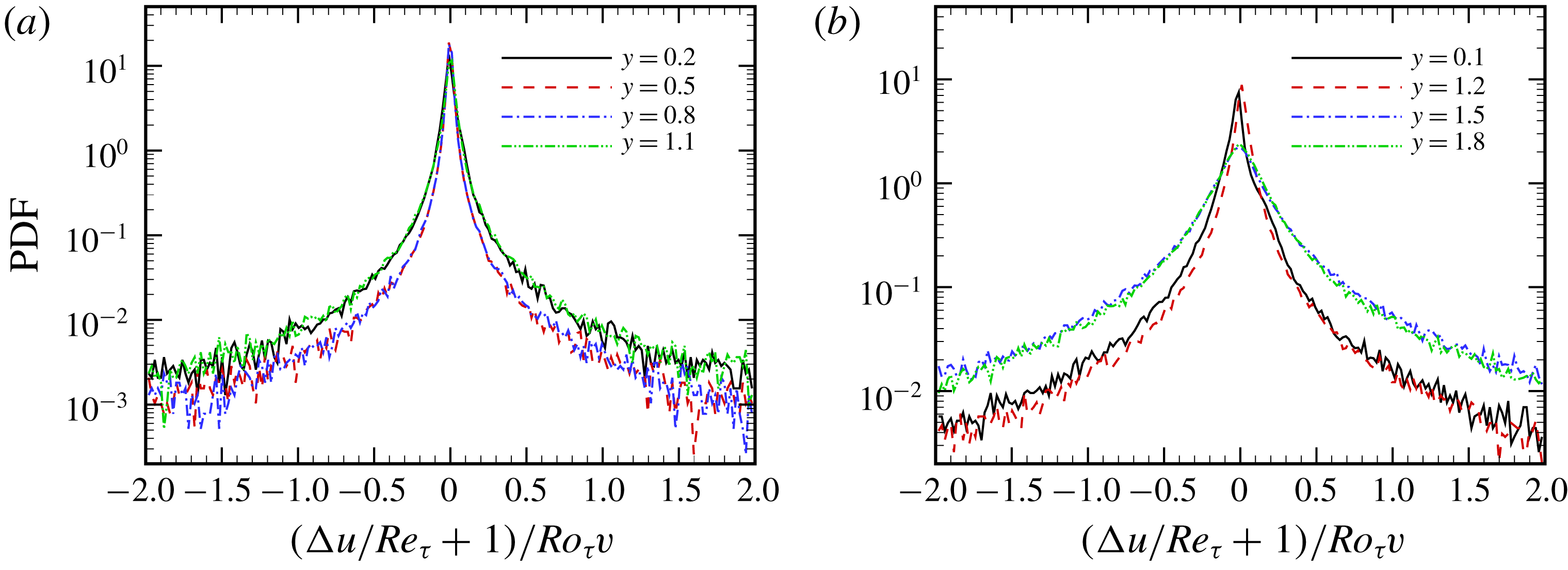
The PDFs of
 $(\unicode[STIX]{x0394}u/Re_{\unicode[STIX]{x1D70F}}+1)/Ro_{\unicode[STIX]{x1D70F}}v$
from the case 2D_Ro40 at different wall-normal locations: (a)
 $y=0.2,0.5,0.8$
and
 $1.1$
; (b)
 $y=0.1,1.2,1.5$
and
 $1.8$
.

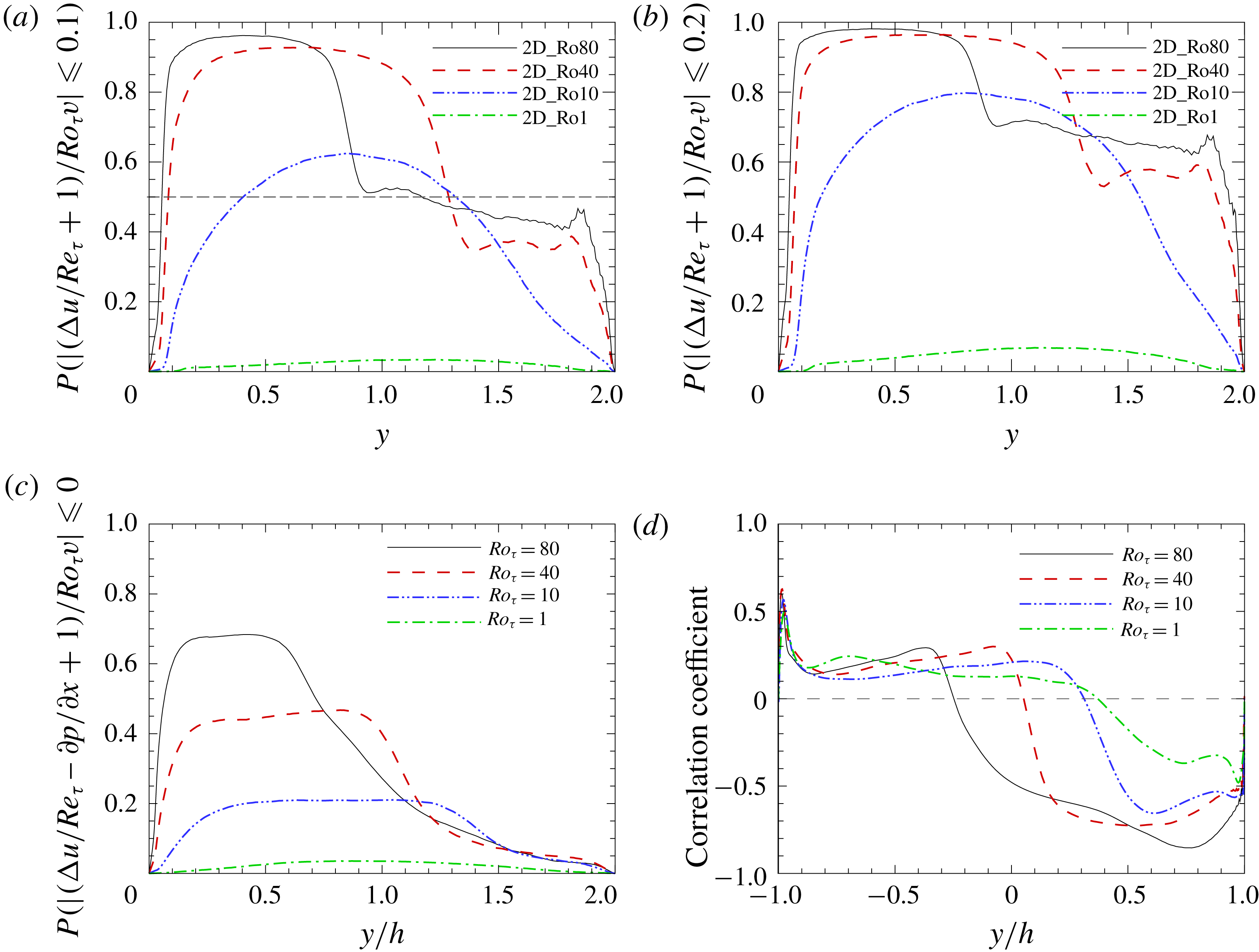
The ratio of points with (a)
 $|(\unicode[STIX]{x0394}u/Re_{\unicode[STIX]{x1D70F}}+1)/Ro_{\unicode[STIX]{x1D70F}}v|\leqslant 0.1$
and (b)
 $|(\unicode[STIX]{x0394}u/Re_{\unicode[STIX]{x1D70F}}+1)/Ro_{\unicode[STIX]{x1D70F}}v|\leqslant 0.2$
to the total points at different
 $y$
from four 2D/3C simulations; (c) the ratio of points with
 $|(\unicode[STIX]{x0394}u/Re_{\unicode[STIX]{x1D70F}}-\unicode[STIX]{x2202}p/\unicode[STIX]{x2202}x+1)/Ro_{\unicode[STIX]{x1D70F}}v|\leqslant 0.2$
to the total points at different
 $y$
from four fully 3-D simulations; (d) the correlation coefficient between
 $(\unicode[STIX]{x0394}u/Re_{\unicode[STIX]{x1D70F}}-\unicode[STIX]{x2202}p/\unicode[STIX]{x2202}x+1)$
and
 $Ro_{\unicode[STIX]{x1D70F}}v$
at different
 $y$
from four fully 3-D simulations.

In order to verify the above arguments, we have to study the ratio
 $(\unicode[STIX]{x0394}u/Re_{\unicode[STIX]{x1D70F}}+1)/Ro_{\unicode[STIX]{x1D70F}}v$
. In figure 8, the probability density functions (PDFs) of
 $(\unicode[STIX]{x0394}u/Re_{\unicode[STIX]{x1D70F}}+1)/Ro_{\unicode[STIX]{x1D70F}}v$
from the case 2D_Ro40 at different wall-normal locations are shown. It is seen that the PDFs have very sharp peaks near
 $(\unicode[STIX]{x0394}u/Re_{\unicode[STIX]{x1D70F}}+1)/Ro_{\unicode[STIX]{x1D70F}}v\approx 0$
. At
 $y=0.5$
and 0.8, the PDFs have the largest peaks. As
 $y$
decreases to 0.2 or 0.1, or it increases to 1.1 or 1.2, the PDFs become wider and their peak values decrease. This trend remains when
 $y$
increases to 1.5 or 1.8. This indicates that there are a lot of points between
 $0.2\leqslant y\leqslant 1.1$
satisfying
 $(\unicode[STIX]{x0394}u/Re_{\unicode[STIX]{x1D70F}}+1)\ll Ro_{\unicode[STIX]{x1D70F}}v$
in the 2D_Ro40 case. More quantitatively, we display in figure 9(a,b) the ratio of points with
 $|(\unicode[STIX]{x0394}u/Re_{\unicode[STIX]{x1D70F}}+1)/Ro_{\unicode[STIX]{x1D70F}}v|\leqslant 0.1$
and
 $|(\unicode[STIX]{x0394}u/Re_{\unicode[STIX]{x1D70F}}+1)/Ro_{\unicode[STIX]{x1D70F}}v|\leqslant 0.2$
to the total points at different
 $y$
from four 2D/3C simulations. It is seen that at
 $Ro_{\unicode[STIX]{x1D70F}}=10$
, 40 and 80, there are a great number of points where
 $|Ro_{\unicode[STIX]{x1D70F}}v|>10|\unicode[STIX]{x0394}u/Re_{\unicode[STIX]{x1D70F}}+1|$
in a certain
 $y$
region where the linear mean velocity profile is observed, and the number of points will increase a lot if the condition is relaxed to
 $|Ro_{\unicode[STIX]{x1D70F}}v|>5|\unicode[STIX]{x0394}u/Re_{\unicode[STIX]{x1D70F}}+1|$
. At
 $Ro_{\unicode[STIX]{x1D70F}}=40$
(or 80), more than 90 % points at
 $0.2<y<1.1$
(
 $0.1<y<0.8$
) satisfy
 $|Ro_{\unicode[STIX]{x1D70F}}v|>10|\unicode[STIX]{x0394}u/Re_{\unicode[STIX]{x1D70F}}+1|$
. On the other hand, there are very few points (less than 10 %) which satisfy
 $|Ro_{\unicode[STIX]{x1D70F}}v|>5|\unicode[STIX]{x0394}u/Re_{\unicode[STIX]{x1D70F}}+1|$
at
 $Ro_{\unicode[STIX]{x1D70F}}=1$
, which is consistent with the fact that the linear mean velocity is not obvious at this rotation number. From these figures, we may say that the assumption
 $|Ro_{\unicode[STIX]{x1D70F}}v|\gg |\unicode[STIX]{x0394}u/Re_{\unicode[STIX]{x1D70F}}+1|$
is valid for most points in the linear mean velocity region, proving the explanation of the linear mean velocity profile.
It should be emphasized that the present explanation for the linear mean velocity profile obtained in the 2D/3C model cannot be extended to fully 3-D cases straightforwardly. In fully 3-D cases, our data showed that the relation
 $|Ro_{\unicode[STIX]{x1D70F}}v|\gg |\unicode[STIX]{x0394}u/Re_{\unicode[STIX]{x1D70F}}-\unicode[STIX]{x2202}p/\unicode[STIX]{x2202}x+1|$
is invalid in most cases. In figure 9(c), the ratio of points with
 $|(\unicode[STIX]{x0394}u/Re_{\unicode[STIX]{x1D70F}}-\unicode[STIX]{x2202}p/\unicode[STIX]{x2202}x+1)/Ro_{\unicode[STIX]{x1D70F}}v|\leqslant 0.2$
to the total points at different
 $y$
from four fully 3-D simulations is shown. It is seen that the ratio increases with rotation number in the linear region, and the highest value is approximately 0.7 at
 $Ro_{\unicode[STIX]{x1D70F}}=80$
. This value is much lower than that from the 2D/3C model, which is more than 0.95. However,
 $(\unicode[STIX]{x0394}u/Re_{\unicode[STIX]{x1D70F}}-\unicode[STIX]{x2202}p/\unicode[STIX]{x2202}x+1)$
is barely correlated with
 $Ro_{\unicode[STIX]{x1D70F}}v$
, as depicted in figure 9(d) where the correlation coefficient of the two terms is only approximately 0.2 in the linear region. In this situation, the additional term
 $(\unicode[STIX]{x0394}u/Re_{\unicode[STIX]{x1D70F}}-\unicode[STIX]{x2202}p/\unicode[STIX]{x2202}x+1)$
on the right-hand side of
 $du/dt$
can be viewed as stochastic forces exerted on the tracers. From this point, the same linear results can be derived approximately.
Recalling the thermal analogy introduced in § 2.2, it is easy to obtain that
 $\langle \hat{\unicode[STIX]{x1D703}}\rangle =-\langle u\rangle +Ro_{\unicode[STIX]{x1D70F}}y$
. Therefore, the linear mean velocity profile also means that the mean temperature is constant in a corresponding region for the special convection problem.
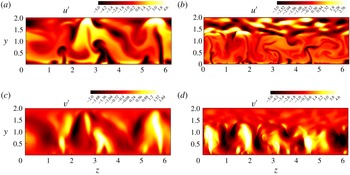
(a,c) Contours of
 $u^{\prime }$
and
 $v^{\prime }$
of an instantaneous field from case 2D_Ro1; (b,d) contours of
 $u^{\prime }$
and
 $v^{\prime }$
of a instantaneous field from case 2D_Ro40.

Plumes are typical structures in thermal convection (Xi, Lam & Xia Reference Xi, Lam and Xia2004; Ahlers et al.
Reference Ahlers, Grossmann and Lohse2009) and were described as both motors and heat pumps that drive the central bulk fluid and transport heat in the system (Kadanoff Reference Kadanoff2001). Since we have shown the analogy between thermal convection and a 2D/3C RPPF with
 $\hat{\unicode[STIX]{x1D703}}=-u+Ro_{\unicode[STIX]{x1D70F}}y$
in § 2.2, we can expect that the contours of the fluctuation of
 $u$
also show plume-like structures in 2D/3C RPPFs. Figure 10(a,b) shows the contours of
 $u^{\prime }$
of an instantaneous field from cases 2D_Ro1 and 2D_Ro40 (see also the supplementary movie 1 and movie 2 available at https://doi.org/10.1017/jfm.2019.715 respectively), and clear plumes can be discerned near the bottom wall as expected. At
 $Ro_{\unicode[STIX]{x1D70F}}=1$
, the plumes can intrude from the one wall to another, while they, although in a thinner and more chaotic form, can only exist at the lower part of the channel at
 $Ro_{\unicode[STIX]{x1D70F}}=40$
. In the other part, there exist chaotic patterns. The corresponding contours of
 $v^{\prime }$
are shown in figure 10(c,d). It is shown that the region where plumes bring up a lower value of
 $u^{\prime }$
has a larger value of
 $v^{\prime }$
.
5 Conclusion
In this paper, a 2D/3C model of spanwise rotating plane Poiseuille flow is introduced. With some derivations, a rigorous analogy can be arrived at between the 2D/3C model and a special 2-D thermal convection with uniform heat sink. Our work shows that the 2D/3C RPPF model is indeed very useful to study flow phenomena in spanwise rotating plane Poiseuille flow.
For the lower Reynolds number case, the model can be used to study the stability behaviours of roll cells in RPPF. With a newly defined Rayleigh number
 $Ra=Re^{2}Ro(3-Ro)^{5}/81$
and channel height
 $H=6/(3-Ro)$
, it is shown that the neutral stability curves, critical eigenfunctions, critical streamfunctions of RPPF at different
 $Ro$
almost collapse. The critical Rayleigh number
 $Ra_{c}$
and critical wavenumber
 $\tilde{a}_{c}$
are nearly constant if
 $H\geqslant 4$
, which in turn can yield analytic expressions for the critical Reynolds number
 $Re_{c}=9\sqrt{1178.6/Ro(3-Ro)^{5}}$
and critical wavenumber
 $a_{c}=3\times 2.034/(3-Ro)$
. These analytic expressions match very well with the numerical simulation results from the present work and previously published ones.
For turbulent states with higher Reynolds numbers, the model is proven to be self-sustained. Direct numerical simulations are carried out, and the results showed that the mean velocity profile from a 2D/3C RPPF exhibits the same linear law near the pressure side as the corresponding fully 3-D RPPF, where the slope of the linear profile equals twice the angular velocity. Thus, we may infer that the linear profiles of the mean velocity and the Reynolds shear stress are dominated by the cross-flow in RPPF. Plume structures are also observed for the fluctuation of
 $u^{\prime }$
.
An explanation as to the linear mean velocity profile is also provided with the assumption that the Coriolis term dominates over the viscous term on the right-hand side of the governing equation for the streamwise component. Our numerical results confirm that the dominant behaviour happens for more than 90 % of points in the linear mean velocity region.
Acknowledgements
The authors would like to thank Dr X. I. A. Yang for many useful discussions and suggestions. This work was supported by the National Science Foundation of China (NSFC grant nos 11822208 and 11772297). The numerical simulations were finished at High-performance Computing Platform of Peking University and the National Supercomputer Centre in Guangzhou (Tianhe-2A), China.
Supplementary movies
Supplementary movies are available at https://doi.org/10.1017/jfm.2019.715.