1. Introduction
Understanding multiphase fluid flow in nanoscale confined spaces is essential for addressing a broad range of scientific and engineering challenges, including unconventional subsurface energy exploitation such as hydraulic fracturing (Mehrabi, Javadpour & Sepehrnoori Reference Mehrabi, Javadpour and Sepehrnoori2017; Wang, Wang & Su Reference Wang, Wang, Su and Jin2022; Minakov, Pryazhnikov & Neverov Reference Minakov, Pryazhnikov, Neverov, Sukhodaev and Zhigarev2024; Zhan, Bao & Wang Reference Zhan, Bao, Wang, Wang, Su, Zhang, Wang and Jin2024), environmental remediation and water purification (Ma, Grey & Shen Reference Ma, Grey, Shen, Urbakh, Wu, Liu, Liu and Zheng2015; Berk & Coletti Reference Berk and Coletti2024), nanomedicine and biomedical engineering (Sanhai, Sakamoto & Canady Reference Sanhai, Sakamoto, Canady and Ferrari2008), materials science (Lowe, Tsyrin & Chorążewski Reference Lowe, Tsyrin, ChorĄżewski, Zajdel, Mierzwa, Leão, Bleuel, Feng, Luo and Li2019), micro-nano-fluidics (Sparreboom, van den Berg & Eijkel Reference Sparreboom, van den Berg and Eijkel2009), sensing (Baptista-Pires, Pérez-López & Mayorga-Martinez Reference Baptista-Pires, Pérez-López, Mayorga-Martinez, Morales-Narváez, Domingo, Esplandiu, Alzina, Sotomayor-Torres and Merkoçi2014) and energy conversion and storage (Smirnov, Vlassiouk & Takmakov Reference Smirnov, Vlassiouk, Takmakov and Rios2010; Gao, Li & Zhang Reference Gao, Li, Zhang, Lu and Xu2020). In such nanoconfined spaces, fluid–fluid and fluid–solid molecular interactions make the mechanisms of multiphase flow highly complex (Wu, Chen & Li Reference Wu, Chen, Li, Li, Xu and Dong2017; Cai, Jiao & Wang Reference Cai, Jiao, Wang, He and Xia2024), posing challenges for conventional continuum-based modelling and highlighting the need for detailed investigations of confined multiphase transport.
These molecular interactions give rise to nanoscale effects, including wall slip, interfacial slip and heterogeneous viscosity, which cause multiphase flow behaviours to deviate significantly from predictions of classical continuum mechanics (Mattia, Leese & Lee Reference Mattia, Leese and Lee2015; Secchi, Marbach & Nigues Reference Secchi, Marbach, Nigues, Stein, Siria and Bocquet2016; Zhan, Su & Jin Reference Zhan, Su, Jin, Zhang, Wang, Hao and Li2020). In continuum fluid mechanics, it is commonly assumed that the tangential velocity at a solid wall is zero, known as the no-slip boundary condition. However, the interactions between fluid molecules and solid surfaces can lead to a finite tangential velocity at the wall, referred to as the slip velocity (Yiotis, Psihogios & Kainourgiakis Reference Yiotis, Psihogios, Kainourgiakis, Papaioannou and Stubos2007; Lasseux, Valdés-Parada & Bottaro Reference Lasseux, Valdés-Parada and Bottaro2021; Lasseux & Valdés-Parada Reference Lasseux and Valdés-Parada2024). This slip velocity is typically described by the Navier slip condition, which relates the slip velocity at the wall to the velocity gradient normal to the wall through a characteristic slip length (Navier Reference Navier1823). Physically, the slip length can be interpreted as the distance inside the solid at which the linear extrapolation of the near-wall velocity profile would reach zero. The non-zero slip velocity is influenced by various factors, including wall wettability (Huang, Sendner & Horinek Reference Huang, Sendner, Horinek, Netz and Bocquet2008; Wang, Javadpour & Feng Reference Wang, Javadpour and Feng2016), surface roughness (Pasquier, Quintard & Davit Reference Pasquier, Quintard and Davit2017; Zhan et al. Reference Zhan, Bao, Wang, Wang, Su, Zhang, Wang and Jin2024), shear rate (Cui Reference Cui2019; Shan, Wang & Wang Reference Shan, Wang, Wang, Zhang and Guo2022), pore size (Thomas & McGaughey Reference Thomas and McGaughey2008; Secchi et al. Reference Secchi, Marbach, Nigues, Stein, Siria and Bocquet2016), temperature (Guo, Zhao & Shi Reference Guo, Zhao and Shi2005) and fluid types (Wu et al. Reference Wu, Chen, Li, Lei, Xu, Wang, Li, Dong, Peng and Yang2019a). Kannam, Todd & Hansen (Reference Kannam, Todd, Hansen and Daivis2013) used equilibrium interfacial-friction calculations together with field-driven non-equilibrium simulations to determine the slip length of water in carbon nanotubes (CNTs), and found that the slip length decreases from approximately 180 nm for 1.66 nm pores to 75 nm for 6.5 nm pores, approaching ∼60 nm for pores ≥ 10 nm. Later, Kannam, Daivis & Todd (Reference Kannam, Daivis and Todd2017) reported that water flow in CNTs (0.8–10 nm) exhibits extremely high and widely scattered slip lengths, ranging from ∼1 to 500 000 nm, due to factors such as the smooth, hydrophobic CNTs’ surface, orientation of OH bonds, low activation energy and reduced interfacial viscosity, and emphasised that accurate determination of the slip length is essential for understanding fluid transport under nanoscale confinement. Secchi et al. (Reference Secchi, Marbach, Nigues, Stein, Siria and Bocquet2016) measured pressure-driven water flow through individual CNTs (15–50 nm) from emerging jets, and deduced exceptionally large radius-dependent slip lengths of approximately 300–20 nm, highlighting the extraordinary interfacial transport inside CNTs. Wettability is closely linked to the strength of fluid–solid molecular interactions and therefore strongly influences the degree of slip at the wall. As surfaces become more non-wetting (i.e. with larger wetting-phase contact angles), the attraction between the fluid and the solid weakens, which tends to reduce interfacial friction and thereby results in a larger slip velocity (Wang et al. Reference Wang, Su, Wang, Sheng, Li and Zafar2019b ). Based on data from numerous experiments and molecular dynamics (MD) simulations, Wu et al. (Reference Wu, Chen, Li, Li, Xu and Dong2017) established quantitative correlations between wettability and slip length, showing that the slip length generally increases with increasing contact angle.
Another important nanoscale effect induced by fluid–solid molecular interactions is the heterogeneity of fluid viscosity in the near-wall region (Chiavazzo, Fasano & Asinari Reference Chiavazzo, Fasano, Asinari and Decuzzi2014; Morciano, Fasano & Nold Reference Morciano, Fasano, Nold, Braga, Yatsyshin, Sibley, Goddard, Chiavazzo, Asinari and Kalliadasis2017). In nanoconfined spaces, the layering and structural ordering of fluid molecules adjacent to solid surfaces can markedly alter their local near-wall viscosity and flow resistance, leading to substantial deviations from those of the bulk phase (Zhang, Li & Sun Reference Zhang, Li, Sun, Feng, Miao, Li and Zhang2017; Qin et al. Reference Qin, Wang, Xia, Ling, Wang and Cai2024a ). Molecular dynamics simulations further reveal that the near-wall region possesses a finite thickness, with the two molecular layers adjacent to the wall being strongly influenced by fluid–solid interactions and causing pronounced viscosity variations. For water, the thickness of this near-wall region is approximately 0.7 nm (Tocci, Joly & Michaelides Reference Tocci, Joly and Michaelides2014; Qin & Buehler Reference Qin and Buehler2015; Neek-Amal, Peeters & Grigorieva Reference Neek-Amal, Peeters, Grigorieva and Geim2016). Consequently, the effective viscosity of the near-wall fluid may be higher or lower than that of the bulk, depending on the fluid type, surface chemistry and wettability (Wu et al. Reference Wu, Chen, Li, Li, Xu and Dong2017; Liu, Yang & Sun Reference Liu, Yang, Sun, Yao and Kou2022; Xu, Zhan & Wang Reference Xu, Zhan, Wang, Su and Wang2022). Petravic & Harrowell, (Reference Petravic and Harrowell2009) demonstrated that shear viscosity near a fluid–solid region can markedly deviate from the bulk value within a narrow interfacial layer using a zero-flux boundary fluctuation approach. Wu et al. (Reference Wu, Chen, Li, Li, Xu and Dong2017) combined the results from experiments and MD simulations to establish a quantitative relationship between interfacial water viscosity, bulk water viscosity and contact angle, showing that for contact angles between 0° and 150°, the near-wall viscosity ranges from approximately 3.25 to 0.55 times the bulk value. Liu et al. (Reference Liu, Yang, Sun, Yao and Kou2022) employed MD simulations of multicomponent alkanes in realistic kerogen nanopores and found that strong kerogen–hydrocarbon affinity produces adsorbed molecular layers and heterogeneous viscosity, thereby causing the near-wall velocity profiles of alkanes to deviate significantly from the typical parabolic shape observed in the bulk region. Such heterogeneous viscosity affects momentum transfer and wall slip, and ultimately governs the macroscopic displacement efficiency of multiphase flow in nanoconfined geometries. Wang et al. (Reference Wang, Su, Wang, Sheng, Li and Zafar2019b ) developed a water flow model in nanopores based on the Hagen–Poiseuille equation in which the wall slip velocity was evaluated from the near-wall viscosity.
In addition to wall slip and heterogeneous viscosity induced by fluid–solid interactions, immiscible fluids in nanoconfined geometries can also exhibit fluid–fluid interfacial slip (Zhan et al. Reference Zhan, Su, Jin, Zhang, Wang, Hao and Li2020; Telari, Tinti & Giacomello Reference Telari, Tinti and Giacomello2022). In such systems, the molecular interactions across the interface are often too weak to fully transmit tangential momentum, resulting in a measurable relative tangential motion between the two fluid phases (Galliero Reference Galliero2010; Xu et al. Reference Xu, Zhan, Wang, Su and Wang2022). Zhan et al. (Reference Zhan, Su, Jin, Zhang, Wang, Hao and Li2020) employed MD simulations to characterise the viscosity of the alkane–water interfacial region using an apparent viscosity, and found that for laminar alkane–water flow in quartz nanopores the interfacial apparent viscosity is approximately 0.22 mPa·s, lower than the viscosities of bulk alkane and water. By non-equilibrium MD, Hilaire, Siboulet & Charton (Reference Hilaire, Siboulet, Charton and Dufrêche2023) showed that heptane–water interfaces exhibit a larger slip length (0.425–1 nm) than those at fluid–solid interfaces due to faster diffusion and lower interfacial friction. This interfacial slip effectively lowers the interfacial shear resistance and can significantly enhance the mobility of the dispersed or non-wetting phase, particularly in the presence of thin wetting films (Wang et al. Reference Wang, Wang, Su and Jin2022). The magnitude of fluid–fluid slip depends on factors such as interfacial tension, molecular affinity, surfactant coverage and the thickness of the interfacial region, and is often quantified in terms of an interfacial slip length or velocity jump typically obtained from MD simulations (Zhan et al. Reference Zhan, Su, Jin, Zhang, Wang, Hao and Li2020).
To date, researchers have investigated the microscopic behaviours of fluid flow in nanoconfined spaces using various approaches, including nanofluidic experiments, MD simulations and pore-scale modelling (Zhang, Javadpour & Yin Reference Zhang, Javadpour, Yin and Li2020; Wang et al. Reference Wang, Zhang, Liu, Ding, Liu, Yao, Sun, Yang, Zhang and Wang2024b ; Zhu, Lu & Pan Reference Zhu, Lu, Pan, Qiao, Raza and Liu2024; Bao, Du & Zhan Reference Bao, Du, Zhan, Wang and Luo2025; Wang et al. Reference Wang, Kang, Wang, He, Xia and Cai2025a ). These studies have provided valuable insights into nanoscale effects such as wall slip, interfacial slip and heterogeneous viscosity. Such nanoscale effects can strongly influence fluid transport, leading to mobility variations several orders of magnitude different from classical continuum models, depending on the strength and combination of wall slip, interfacial slip and heterogeneous viscosity (Majumder, Chopra & Andrews Reference Majumder, Chopra, Andrews and Hinds2005; Holt, Park & Wang Reference Holt, Park, Wang, Stadermann, Artyukhin, Grigoropoulos, Noy and Bakajin2006; Secchi et al. Reference Secchi, Marbach, Nigues, Stein, Siria and Bocquet2016; Wu et al. Reference Wu, Chen, Li, Xu, Wang, Li, Wang and Dong2019b ; Qin et al. Reference Qin, Wu, Xia, Wang and Cai2024b ; Zhou, Neek-Amal & Peeters Reference Zhou, Neek-Amal, Peeters, Bai and Sun2024). The enhancement factor is commonly employed to quantify the influence of nanoscale effects on flow capacity, defined as the ratio of the flow flux calculated with nanoscale effects to that without, with reported values ranging from 0.1 to 107. Wu et al. (Reference Wu, Chen, Li, Li, Xu and Dong2017) developed a theoretical nanopore flow model by fitting extensive molecular simulation and experimental data, showing that the enhancement factor can reach up to 107 at contact angles approaching 180° under idealised conditions. Zhao, Kang & Yao (Reference Zhao, Kang, Yao, Zhang, Li, Yang and Sun2018) and Qin et al. (Reference Qin, Wu, Xia, Wang and Cai2024b ) employed the lattice Boltzmann method (LBM) and the finite volume method to investigate water flow in nanoporous media. The results showed that, at a water contact angle of 0°, the enhancement factor is approximately 0.8, which is mainly attributed to the significantly increased near-wall water viscosity. In contrast, when the contact angle increases to 150°, the enhancement factor can reach values up to 9, primarily because of the enhanced wall slip. Such a wide range of contact angles is physically relevant in subsurface systems, as wettability can be altered not only by surfactants or other chemical agents (Minakov et al. Reference Minakov, Pryazhnikov, Neverov, Sukhodaev and Zhigarev2024; Vaganov, Zhigarev & Pryazhnikov Reference Vaganov, Zhigarev, Pryazhnikov, Shebeleva, Nemtsev and Minakov2025), but also by the intrinsic mineralogical heterogeneity of nanoporous media (Hu, Liu & Zhang Reference Hu, Liu, Zhang, Song, Thaika, Li, Kuru, Shi and Liu2024; Zhu et al. Reference Zhu, Lu, Pan, Qiao, Raza and Liu2024). In particular, hydrophilic minerals such as quartz and clays often coexist with hydrophobic organic matter (e.g. kerogen), leading to pronounced pore-scale wettability variations (Xu, Yang & Kang Reference Xu, Yang, Kang, Nie and Fu2026). However, the majority of existing studies have primarily focused on single-phase flow in nanoporous media, while investigations of two-phase flow in nanoconfined spaces remain relatively limited. Zhan et al. (Reference Zhan, Su, Jin, Zhang, Wang, Hao and Li2020) and Xu et al. (Reference Xu, Zhan, Wang, Su and Wang2022) examined stratified two-phase flow within a single nanopore based on MD simulations and reported that interfacial slip can yield an enhancement factor of approximately 1.2. However, these studies are largely restricted to single nanopores and simplified fluid distributions, and therefore remain insufficient to capture the coupled nanoscale effects governing multiphase transport in complex nanoporous media, especially under varying phase distributions, wettability conditions and capillary numbers. Feng, Li & Wang (Reference Feng, Li, Wang, Li, Zhang, Sun, He, Liu, Qin and Han2018) revisited the Lucas–Washburn theory by incorporating near-wall viscosity and wall slip length to analyse capillary filling in nanopores, revealing that both wettability and geometric factors exert a significant influence on the filling dynamics. In our previous work (Wang et al. Reference Wang, Wang, Su and Jin2022), a nanoscale lattice Boltzmann (LB) framework incorporating molecular interactions was developed based on fitted MD results to investigate periodic two-phase flow in simplified porous structures and to evaluate the impact of nanoscale effects on relative permeability. However, in many scientific and engineering applications, nanoporous media are characterised by highly complex pore structures, for which the simplified pore models fail to accurately capture the multiphase flow behaviour. Furthermore, transport in nanoporous media is primarily driven by displacement and replacement processes rather than the periodic dynamics, posing significant challenges for elucidating interfacial characteristics during displacement.
In this work, the objective is to develop an accurate nanoscale pseudopotential LB framework that explicitly incorporates the molecular interactions responsible for wall slip, interfacial slip and heterogeneous viscosity, and to apply this framework to investigate multiphase displacement in nanoporous media under a wide range of conditions. The considered test cases are designed to represent typical multiphase transport configurations in nanoporous media relevant to unconventional subsurface reservoirs and are primarily intended for mechanistic understanding rather than direct field-scale prediction or quantitative upscaling.
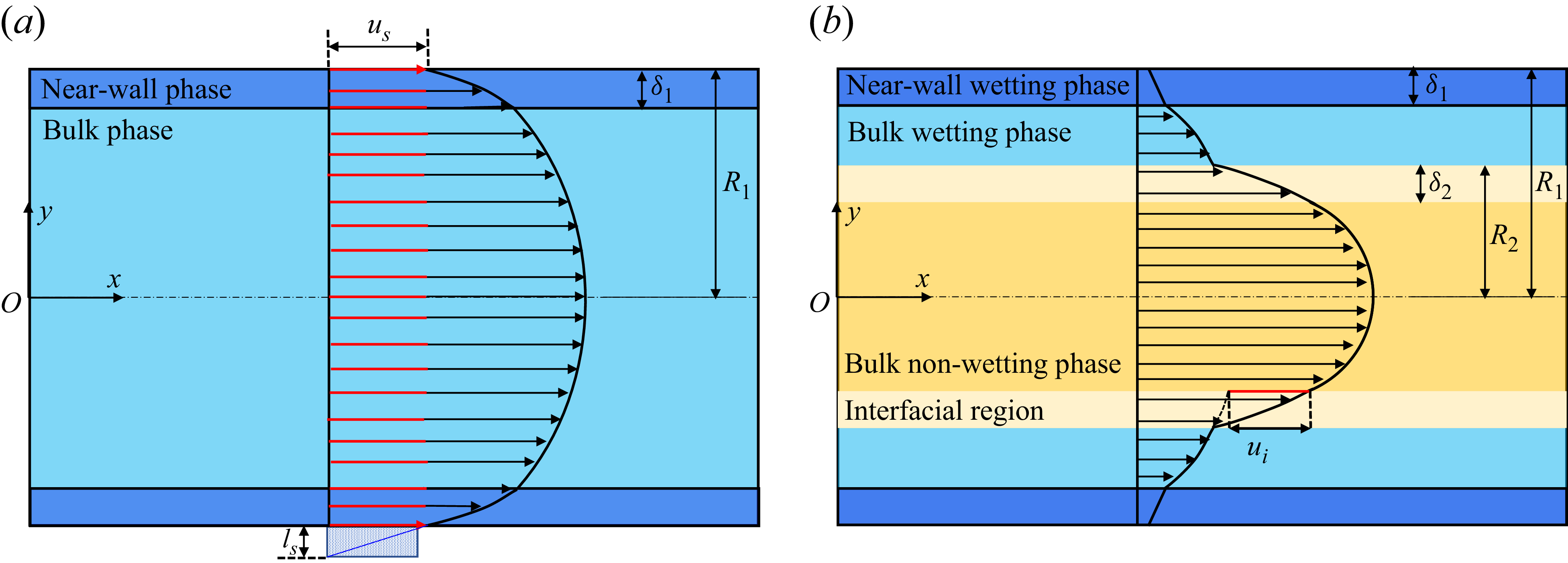
Schematic diagram of the velocity profiles of single-phase flow (a) and stratified two-phase flow (b) in circular nanopores.

The remainder of the paper is organised as follows. In § 2, the theory of fluid transport in nanoconfined spaces and the LB framework for two-phase flow, together with the treatment of nanoporous media and multiphase distribution, are described in detail. Model validation and parameter calibration from MD simulations are presented in § 3. In § 4, the effects of molecular interactions under varying initial wetting-phase saturation, wettability and capillary number (Ca) are systematically analysed, including an assessment of the robustness of nanoscale effects across different nanoporous structures and the identification of a universal scaling behaviour linking enhancement factor and displacement efficiency. Finally, concluding remarks are given in § 5.
2. Model development
2.1. Theory of fluid transport in nanoconfined spaces
In conventional pores, typically at the micrometre scale or larger, laminar flow exhibits a velocity distribution that follows the classical Hagen–Poiseuille (HP) law, yielding a characteristic parabolic profile. As illustrated in figure 1(a), when the pore radius decreases to the nanometre scale, molecular interactions at the fluid–solid interface give rise to a finite wall slip velocity (
 $u_{s}$
), while viscosity heterogeneity in the near-wall region induces variations in the local velocity gradient. The resulting velocity profile can be represented by two sets of HP equations (Mattia & Calabrò Reference Mattia and Calabrò2012), separately describing the near-wall and bulk fluids, as expressed in (2.1) and (2.2)
 \begin{align} u_{n}(r)=\frac{{R}_{1}^{2}-r^{2}}{4\mu _{n}}\boldsymbol{\nabla }\!p+C_{1},R_{1}-\delta _{1}\leq r\leq R_{1} , \\[-28pt] \nonumber \end{align}
 \begin{align} u_{b}(r)=\frac{{R}_{1}^{2}-r^{2}}{4\mu _{b}}\boldsymbol{\nabla }\!p+C_{2},0\leq r\leq R_{1}-\delta _{1} , \\[0pt] \nonumber \end{align}
where
 $u_{n}$
and
 $u_{b}$
are the velocities of the near-wall and bulk fluids, the subscripts n and b indicate the near-wall and bulk region,
 $R_{1}$
is the pore radius,
 $\delta _{1}$
is the thickness of near-wall region,
 $\boldsymbol{\nabla }\!p$
is pressure gradient,
 $\mu _{n}$
and
 $\mu _{b}$
are the viscosities of near-wall and bulk fluids,
 $r$
is the vertical distance from the central axis of the nanopore and
 $C_{1}$
and
 $C_{2}$
are coefficients related to the molecular interactions, which can be determined by the conditions of wall slip velocity and velocity continuity, with the detailed derivation provided in Appendix A.
Extending the single-phase flow to a two-phase system, figure 1(b) shows that a stratified two-phase flow in a nanopore can be divided into four regions: the near-wall wetting phase, the bulk wetting phase, the fluid–fluid interface and the bulk non-wetting phase (Wang et al. Reference Wang, Su, Wang, Li, Sheng and Zhan2019a
). In addition to wall slip and heterogeneous near-wall viscosity, an interfacial slip velocity (
 $u_{i}$
) also arises at the interfacial region. Accordingly, the velocity distribution can be represented by four sets of HP equations corresponding to these regions, as expressed in (2.3)–(2.6)
 \begin{align} u_{nw}(r)=\frac{{R}_{1}^{2}-r^{2}}{4\mu _{nw}}\boldsymbol{\nabla }\!p+C_{3}, \left(R_{1}-\delta _{1}\right)\lt r\leq R_{1} , \\[-28pt] \nonumber \end{align}
 \begin{align} u_{bw}(r)=\frac{{R}_{1}^{2}-r^{2}}{4\mu _{bw}}\boldsymbol{\nabla }\!p+C_{4}, R_{2}\lt r\leq \left(R_{1}-\delta _{1}\right) , \\[-28pt] \nonumber \end{align}
 \begin{align} u_{i}(r)=\frac{{R}_{1}^{2}-r^{2}}{4\mu _{i}}\boldsymbol{\nabla }\!p+C_{5}, \left(R_{2}-\delta _{2}\right)\lt r\leq R_{2} , \\[-28pt] \nonumber \end{align}
 \begin{align} u_{bnw}(r)=\frac{{R}_{1}^{2}-r^{2}}{4\mu _{bnw}}\boldsymbol{\nabla }\!p+C_{6},0\leq r\leq \left(R_{2}-\delta _{2}\right) , \\[0pt] \nonumber \end{align}
where
 $u_{nw} , u_{bw} , u_{i}$
and
 $u_{bnw}$
are the velocities of near-wall wetting, bulk wetting, interfacial and bulk non-wetting fluids,
 $\mu _{nw} , \mu _{bw} , \mu _{i}$
and
 $\mu _{bnw}$
are the viscosities of near-wall wetting, bulk wetting, interfacial and bulk non-wetting fluids,
 $\delta _{2}$
is the thickness of interfacial region,
 $R_{2}$
denotes the radius of the non-wetting-phase region, covering the interfacial and the bulk non-wetting-phase regions and
 $C_{3} , C_{4} , C_{5} , C_{6}$
are coefficients related to the molecular interactions, which can be obtained from the interfacial and boundary continuity conditions, with the detailed derivation provided in Appendix B. The formulation presented above characterises the velocity profiles within circular pores. The analogous analytical solutions for flow in two-dimensional slit pores, which correspond directly to the two-dimensional LB simulations, are detailed in Appendix C.
2.2. Lattice Boltzmann method for two-phase flow in nanoconfined spaces
Based on the above theoretical framework, a multiphase and multicomponent pseudopotential LBM is adopted to simulate two-phase displacement in nanoconfined spaces. This approach enables us to capture the combined effects of wall slip, interfacial slip and heterogeneous viscosity at the pore scale (Wang et al. Reference Wang, Wang, Su and Jin2022). The governing equations are given as follows (Lallemand & Luo Reference Lallemand and Luo2000; Guo, Zheng & Shi Reference Guo, Zheng and Shi2002):
 \begin{align} {\boldsymbol{f}}_{\!\sigma }^{*} (\boldsymbol{x},t)=\boldsymbol{f}_{\!\sigma } (\boldsymbol{x},t)-\boldsymbol{M}^{-1}\boldsymbol{\varLambda }\left(\boldsymbol{m}_{\sigma } (\boldsymbol{x},t)-{\boldsymbol{m}}_{\sigma }^{\textit{eq}} (\boldsymbol{x},t)\right)+\delta _{t}\boldsymbol{M}^{-1}\left(\boldsymbol{I}-\frac{\boldsymbol{\varLambda }}{2}\right)\boldsymbol{S}_{\sigma } , \end{align}
where
 $\boldsymbol{f}_{\!\sigma }(\boldsymbol{x},t)$
is the particle distribution function of
 $\sigma$
phase at
 $\boldsymbol{x}$
position and time
 $t , \boldsymbol{M}$
is the transformation matrix,
 $\boldsymbol{\varLambda }$
is the relaxation diagonal matrix,
 $\boldsymbol{m}_{\sigma }=\boldsymbol{M}\!\boldsymbol{f}_{\!\sigma } , {\boldsymbol{m}}_{\sigma }^{\textit{eq}}=\boldsymbol{M}\!{\boldsymbol{f}}_{\!\sigma }^{\textit{eq}}$
denote the particle distribution function in moment space and the corresponding equilibrium distribution function,
 $\delta _{t}$
is the time step,
 $\boldsymbol{I}$
is the unit matrix and
 $\boldsymbol{S}_{\sigma }$
is the forcing term in the moment space. The streaming process can be expressed as
 $\boldsymbol{f}_{\!\sigma }(\boldsymbol{x}+\boldsymbol{e}_{\alpha }\delta _{t},t+\delta _{t})={\boldsymbol{f}}_{\!\sigma }^{*}(\boldsymbol{x},t)$
where
 $\boldsymbol{e}_{\alpha }$
denotes the discrete lattice velocity, and
 $\alpha =0,1,2,\ldots ,8$
are the nine directions of the two-dimensional nine-velocity model.
The transformation matrix
 $\boldsymbol{M}$
is defined as
 \begin{align} \boldsymbol{M}=\left[\begin{array}{c@{\quad}c@{\quad}c@{\quad}c@{\quad}c@{\quad}c@{\quad}c@{\quad}c@{\quad}c} 1 & 1 & 1 & 1 & 1 & 1 & 1 & 1 & 1\\[5pt] -4 & -1 & -1 & -1 & -1 & 2 & 2 & 2 & 2\\[5pt] 4 & -2 & -2 & -2 & -2 & 1 & 1 & 1 & 1\\[5pt] 0 & 1 & 0 & -1 & 0 & 1 & -1 & -1 & 1\\[5pt] 0 & -2 & 0 & 2 & 0 & 1 & -1 & -1 & 1\\[5pt] 0 & 0 & 1 & 0 & -1 & 1 & 1 & -1 & -1\\[5pt] 0 & 0 & -2 & 0 & 2 & 1 & 1 & -1 & -1\\[5pt] 0 & 1 & -1 & 1 & -1 & 0 & 0 & 0 & 0\\[5pt] 0 & 0 & 0 & 0 & 0 & 1 & -1 & 1 & -1 \end{array}\right] \! . \end{align}
The forcing term in the moment space
 $\boldsymbol{S}_{\sigma }$
is given by
 \begin{align} \boldsymbol{S}_{\sigma }=\left[\begin{array}{cccccccccc} 0\\[5pt] 6\left({u}_{\sigma ,x}^{\textit{eq}}F_{\sigma ,x}+{u}_{\sigma ,y}^{\textit{eq}}F_{\sigma ,y}\right)\\[5pt] -6\left({u}_{\sigma ,x}^{\textit{eq}}F_{\sigma ,x}+{u}_{\sigma ,y}^{\textit{eq}}F_{\sigma ,y}\right)\\[5pt] F_{\sigma ,x}\\[5pt] -F_{\sigma ,x}\\[5pt] F_{\sigma ,y}\\[5pt] -F_{\sigma ,y}\\[5pt] 2\left({u}_{\sigma ,x}^{\textit{eq}}F_{\sigma ,x}-{u}_{\sigma ,y}^{\textit{eq}}F_{\sigma ,y}\right)\\[5pt] \left({u}_{\sigma ,x}^{\textit{eq}}F_{\sigma ,y}+{u}_{\sigma ,y}^{\textit{eq}}F_{\sigma ,x}\right) \end{array}\right] , \end{align}
where
 ${\boldsymbol{u}}_{\sigma }^{\textit{eq}}=({u}_{\sigma ,x}^{\textit{eq}},{u}_{\sigma ,y}^{\textit{eq}})$
is the equilibrium velocity, that can be calculated as
 \begin{align} {\boldsymbol{u}}_{\sigma }^{\textit{eq}}=\frac{\sum _{\sigma }\!\rho _{\sigma }\boldsymbol{u}_{\sigma }}{\sum _{\sigma }\!\rho _{\sigma }} . \end{align}
The velocity
 $\boldsymbol{u}_{\sigma }$
of component
 $\sigma$
can be expressed by
 \begin{align} \boldsymbol{u}_{\sigma }=\left(u_{\sigma ,x},u_{\sigma ,y}\right)=\frac{\sum _{\alpha }\boldsymbol{e}_{\alpha }f_{\sigma ,\alpha }+0.5\delta _{t}\!\boldsymbol{F}_{\!\sigma }}{\rho _{\sigma }} , \end{align}
where
 $\boldsymbol{F}_{\!\sigma }=(F_{\sigma ,x},F_{\sigma ,y})=\boldsymbol{F}_{\sigma ,\textit{int}}+\boldsymbol{F}_{\sigma ,\textit{ads}}+\boldsymbol{F}_{\sigma ,\textit{b}}$
is the total force, composed of the fluid–fluid interaction force
 $\boldsymbol{F}_{\sigma ,\textit{int}}$
, the fluid–solid interaction force
 $\boldsymbol{F}_{\sigma ,\textit{ads}}$
and the external body force
 $\boldsymbol{F}_{\sigma ,\textit{b}}$
, and the force can be expressed as (Shan & Chen Reference Shan and Chen1993; Martys & Chen Reference Martys and Chen1996; Chen, Kang & Mu Reference Chen, Kang, Mu, He and Tao2014)
 \begin{align} \boldsymbol{F}_{\sigma ,\textit{int}} (\boldsymbol{x},t)& =-G_{\sigma \sigma '}\psi _{\sigma } (\boldsymbol{x},t)\sum _{\alpha }w\big(| \boldsymbol{e}_{\alpha }| ^{2}\big)\psi _{\sigma '}\left(\boldsymbol{x}+\boldsymbol{e}_{\alpha }\delta _{t}\right)\boldsymbol{e}_{\alpha } \nonumber \\ & \quad -G_{\sigma \sigma }\psi _{\sigma } (\boldsymbol{x},t)\sum _{\alpha }w \big(| \boldsymbol{e}_{\alpha }| ^{2}\big)\psi _{\sigma }\left(\boldsymbol{x}+\boldsymbol{e}_{\alpha }\delta _{t}\right)\boldsymbol{e}_{\alpha } , \\[-28pt] \nonumber \end{align}
 \begin{align} \boldsymbol{F}_{\sigma ,\textit{ads}} (\boldsymbol{x},t) & =-G_{\sigma s}\psi _{\sigma } (\boldsymbol{x},t)\sum _{\alpha }w\big(| \boldsymbol{e}_{\alpha }| ^{2}\big)s\left(\boldsymbol{x}+\boldsymbol{e}_{\alpha }\delta _{t}\right)\boldsymbol{e}_{\alpha } , \\[-28pt] \nonumber \end{align}
 \begin{align} \boldsymbol{F}_{\sigma ,\textit{b}}=\left(F_{\sigma ,\textit{b},x},F_{\sigma ,\mathrm{b},y}\right) , \\[0pt] \nonumber \end{align}
where
 $G_{\sigma \sigma '}$
is fluid–fluid interaction force parameter, and
 $G_{\sigma \sigma '}=2.3$
. Here,
 $\psi _{\sigma }=1-\exp (-\rho _{\sigma })$
is a pseudopotential,
 $w(| \boldsymbol{e}_{\alpha }| ^{2})$
is the weight and
 $w(1)=1/3 , w(2)=1/12$
and
 $G_{\sigma \sigma }$
is the internal interaction force of
 $\sigma$
phase, which is set to –0.9 for the wetting phase and 0 for the non-wetting phase to capture a low density ratio (= 0.8). The parameter
 $G_{\sigma s}$
is the fluid–solid interaction force parameter and
 $s(\boldsymbol{x}+\boldsymbol{e}_{\alpha }\delta _{t})$
is an indicator parameter that equals 0 and 1 for fluid and solid regions, respectively.
Li, Li & Yan (Reference Li, Li, Yan, Galindo-Torres, Scheuermann and Li2021) demonstrated that a spatially exponentially decaying fluid–solid interaction force can capture long-range molecular forces, leading to a depletion layer and intrinsic apparent slip. However, this framework is primarily tailored for simple geometries (e.g. confined parallel-plate channels) and presents limitations for complex porous media. In this study, the classic pseudopotential fluid–solid interaction scheme is employed. Unlike the spatially decaying force model, the interaction force in our simulation is derived from a constant solid and fluid density assigned to all nodes. Consequently, this interaction results in a constant force value at the interface that does not inherently generate the physical slip. For modelling of the two-phase slip boundary condition, this study employs a modified hybrid boundary scheme combining the half-way bounce-back and diffusive Maxwell reflection models proposed in our previous work, which is expressed as follows (Wang et al. Reference Wang, Wang, Su and Jin2022):
 \begin{align} f_{\sigma ,\alpha }=\left(1-r_{\sigma }\right)\overline{f_{\sigma ,\overline{\alpha }}}+r_{\sigma }\frac{\sum _{\alpha }s\left(\boldsymbol{x}+\boldsymbol{e}_{\alpha }\delta _{t}\right)\overline{f_{\sigma ,\overline{\alpha }}}}{\sum _{\alpha }s\left(\boldsymbol{x}+\boldsymbol{e}_{\alpha }\delta _{t}\right){f}_{\sigma ,\alpha }^{\textit{eq}}\left(0\right)}{f}_{\sigma ,\alpha }^{\textit{eq}}\left(0\right) , \end{align}
where
 $r_{\sigma }$
is the combined slip parameter,
 $\overline{f_{\sigma ,\overline{\alpha }}}$
is the post-collision density distribution function in direction
 $\overline{\alpha }$
and
 $\overline{\alpha }$
is the inverse direction of direction
 $\alpha$
.
For heterogeneous viscosity conditions, the fluid properties in the near-wall and bulk regions can be determined from molecular simulations, and different relaxation times are then assigned to these regions within the LB framework. Specifically, the relaxation diagonal matrix
 $\boldsymbol{\varLambda }$
is defined as
 \begin{align} \boldsymbol{\varLambda }=\text{diag}(s_{0},s_{1},s_{2},s_{3},s_{4},s_{5},s_{6},s_{7},s_{8}) , \end{align}
where
 $s_{7}$
and
 $s_{8}$
are relaxation rates directly related to the relaxation time
 $\tau _{\sigma }$
, and
 $s_{7}=s_{8}=s_{v}=1/\tau _{\sigma }$
. The parameter
 $\tau _{\sigma }$
is related to the kinematic viscosity, and
 $v_{\sigma }={c}_{\textit{s}}^{2}\delta _{\textit{t}}(\tau _{\sigma }-0.5)$
. The remaining relaxation rates are given as
 $s_{0}=s_{3}=s_{5}=s_{6}=1 , s_{1}=s_{2}=s_{4}=1.1$
. For heterogeneous viscosity systems, distinct relaxation parameters are introduced for the bulk and near-wall fluids, denoted by
 $\tau _{\sigma -\textit{b}}$
and
 $\tau _{\sigma -{w}}$
, respectively. The corresponding kinematic viscosities
 $v_{\sigma -\textit{b}}$
and
 $v_{\sigma -{w}}$
are expressed as
 \begin{align} v_{\sigma -\textit{b}}={c}_{\textit{s}}^{2}\delta _{\textit{t}}\left(\tau _{\sigma -\textit{b}}-0.5\right) , \\[-28pt] \nonumber \end{align}
 \begin{align} v_{\sigma -{w}}={c}_{\textit{s}}^{2}\delta _{\textit{t}}\left(\tau _{\sigma -{w}}-0.5\right) . \\[0pt] \nonumber \end{align}
In conventional LB simulations of multiphase flow, the velocity is typically assumed to be continuous across the fluid–fluid interface, which makes it difficult to directly capture interfacial slip. However, MD simulations and theoretical studies have demonstrated that interfacial slip can be effectively captured by introducing an apparent viscosity within the interfacial region, thereby inducing a velocity discontinuity between the two phases. To incorporate this effect into the LB framework, the relaxation time of fluids in the interfacial region is modified accordingly (Wang et al. Reference Wang, Wang, Su and Jin2022). The phase-field variable
 $\rho ^{N}=(\rho _{\sigma }-\rho _{\overline{\sigma }})/(\rho _{\sigma }+\rho _{\overline{\sigma }})$
, which is commonly employed in the colour-gradient LBM to characterise the interface, is used here to define the interfacial region, within which the relaxation time is adjusted to reproduce interfacial slip. The governing expression is given as follows:
 \begin{align} s_{v}= \begin{cases} 1/\tau _{\sigma } & \rho ^{N}\gt \delta,\\[5pt] 1/\tau _{i} & \delta \gt \left| \rho ^{N}\right| \gt 0, \\[4pt] 1/\tau _{\sigma '} & \rho ^{N}\lt -\delta , \end{cases} \end{align}
where
 $\delta$
is a parameter controlling the interfacial thickness and
 $\tau _{i}$
is the relaxation time of the interfacial region.
Based on the densities and pseudopotentials of the two phases, the pressure p of the simulation system can be calculated as
 \begin{align} p={c}_{s}^{2}\left(\rho _{\sigma }+\rho _{\sigma '}\right)+2{c}_{s}^{2}G_{\sigma \sigma '}\psi _{\sigma }\psi _{\sigma '}+\frac{{c}_{s}^{2}}{2}G_{\sigma \sigma }{\psi }_{\sigma }^{2} . \end{align}
2.3. Porous media, initial conditions and multiphase distributions
Based on shale core samples from the Sichuan Basin, high-resolution microstructural images are acquired using scanning electron microscopy (SEM). The core surface is divided into multiple subregions and scanned sequentially, and the resulting SEM images are automatically stitched together using the modular automated processing system (MAPS). This procedure yielded a continuous large-area MAPS image with a spatial extent of 3.119 × 1.859 mm2, as shown in figure 2(a). From the MAPS image, a representative pore–fracture region is selected for pore-scale modelling, as illustrated in figure 2(b). The pore and microfracture structures are then extracted from the SEM image using a threshold-based segmentation approach, resulting in an initial two-dimensional pore–fracture distribution, as shown in figure 2(c). Unlike three-dimensional digital rock reconstructions, pore structures directly extracted from two-dimensional SEM images often exhibit poor connectivity and are therefore unsuitable for multiphase flow simulations. To address this limitation, a watershed algorithm is employed to connect isolated pores and fractures, thereby ensuring global connectivity of the pore network, as shown in figure 2(d). Subsequently, the pore connectivity is further refined based on typical coordination numbers of unconventional reservoir rocks (generally less than 3), in order to eliminate non-physical overconnections and preserve realistic pore-network topology. The final two-dimensional nanoporous medium used for simulations is shown in figure 2(e). It should be noted that the nanoscale effects on flow capacity are strongly dependent on pore size. Previous studies have shown that, when pore or fracture apertures exceed approximately 100 nm, nanoscale effects such as wall slip, interfacial slip and heterogeneous viscosity become significantly weakened (Wu et al. Reference Wu, Chen, Li, Li, Xu and Dong2017). To ensure that nanoscale effects remain dominant while preserving the realistic pore–fracture topology, the extracted pore structure is uniformly rescaled in size. After scaling, the computational domain measures 990 × 600 nm2, corresponding to a lattice resolution of 4950 × 3000 lu2 in the LB framework. Unless otherwise stated, all quantities in the LB simulations are expressed in lattice units (lu), time is reported in lattice time units (lt). The majority of pore diameters fall within the range of 5–30 nm, as shown in figure 2(f). This pore size distribution lies well within the regime in which molecular-interaction-induced effects are expected to play a critical role in multiphase transport.
Image-based reconstruction and characterisation of pore–fracture structures, point-to-wall distance, pore size distribution and idealised porous media. (a) Large-area MAPS image reconstructed from sequential SEM scans. (b) Selected representative pore–fracture region extracted from the MAPS image. (c) Initial pore–fracture structure obtained by threshold segmentation. (d) Globally connected pore–fracture network generated using the watershed algorithm. (e) Final reconstructed porous medium after coordination-number correction, with the point-to-wall distance field illustrated. (f) Pore size distribution. (g) Additional idealised porous medium 1 with regular pore array. (h) Additional idealised porous medium 2 with randomly distributed circular-pore structure. (i) Additional idealised porous medium 3 with irregular pore structure.

To assess the robustness of the simulation results and to exclude potential structural bias associated with a single-pore geometry, three additional idealised nanoporous media are constructed for comparison. These include a regular pore array, a randomly distributed circular-pore structure and an irregular pore structure, as shown in figure 2(g–i), respectively. By repeating multiphase displacement simulations in these different nanoporous media, the generality of the observed nanoscale effects on multiphase flow behaviour can be systematically evaluated.
In natural reservoirs, varying connate water saturations are common and strongly influence subsequent two-phase flow processes. To account for this effect, initial water (as the wetting phase) saturations
 $S_{w}$
of 0, 0.1, 0.2 and 0.3 are imposed to the following LB simulations. For the reference case with
 $S_{w}=0$
, as illustrated in figure 3(a), periodic boundary conditions are imposed at the top, bottom, left and right boundaries of the nanoporous medium. The porous domain is initially saturated with the non-wetting phase, while a reservoir of the wetting phase is placed at the left side of the domain. A uniform body force is applied to the fluid to drive the displacement process through the nanoporous medium. The periodic flow induced by the applied body force ensures mass conservation throughout the simulation.
Initial two-phase distributions for different
 $S_{w}$
conditions (red: non-wetting phase, blue: wetting phase). (a) Initial condition and two-phase distribution at
 $S_{w}=0$
. (b) Temporal evolution of two-phase distribution at
 $S_{w}=0.2$
. (c) Resulting initial two-phase distributions at
 $S_{w}=0.1$
and
 $S_{w}=0.3$
, where T denotes the end time of the periodic flow stage at which the resulting initial two-phase distributions are obtained.

For cases with non-zero initial water saturation, the nanoporous media are initially occupied by a two-phase system. Figure 3(b) illustrates the procedure for generating an initial distribution corresponding to an initial saturation
 $S_{w}=0.2$
. Specifically, a prescribed fraction of the wetting phase is initially distributed randomly within the pore space of the nanoporous medium. A uniform body force is then applied to drive the two-phase mixture to flow periodically through the nanoporous medium, during which the water spontaneously coalesces and preferentially accumulates along the pore walls. Once the wetting-phase distribution reaches a stable configuration, the resulting two-phase pattern is adopted as the initial condition for the corresponding case of
 $S_{w}=0.2$
. Using the same approach, initial distributions for
 $S_{w}=0.1$
and 0.3 are generated, and the corresponding two-phase distributions for the following simulation are given in figure 3(c).
Velocity profiles in a single quartz nanopore: comparison among MD simulations, LB simulations and theoretical predictions. (a) Single-phase flow of the non-wetting n-alkanes (Wang et al. Reference Wang, Wang, Su and Jin2022). (b) Single-phase flow of the wetting water phase (Wang et al. Reference Wang, Wang, Su and Jin2022). (c) Stratified two-phase flow of non-wetting n-alkanes and wetting water phase (Zhan et al. Reference Zhan, Su, Jin, Zhang, Wang, Hao and Li2020).

3. Model validation and parameter calibration
Molecular dynamics simulations can accurately capture intermolecular interactions under nanoconfinement, and thus provide detailed insights into the physicochemical behaviour of confined fluids. Consequently, MD results serve as a reliable benchmark for validating and calibrating the pore-scale LB framework proposed in this study. In the context of shale reservoir development, extensive MD investigations have been conducted on the flow behaviour of n-alkane–water systems in nanopores associated with different mineral types. Figures 4(a) and 4(b) present MD-derived velocity profiles of single-phase flows in quartz nanopores for a non-wetting n-alkane phase and a wetting water phase. For the non-wetting n-alkane phase, a distinct non-zero slip velocity is observed at the solid boundary, while the wetting water phase exhibits pronounced velocity gradient variations in the near-wall region, primarily due to heterogeneous viscosity effects. By adjusting the wall slip parameter in (2.15) and the heterogeneous viscosity terms in (2.17) and (2.18), and applying a uniform body force to drive flow, the LB simulations successfully reproduce the velocity distributions shown in figures 4(a) and 4(b). Although both LB and MD simulations yield consistent velocity distributions, the slip length cannot be directly extracted from the profiles. Instead, it is determined by adjusting the slip length
 $l_{s}$
in equations (C1) and (C2) detailed in Appendix C to fit the simulated velocity profiles, thereby enabling a quantitative estimation of
 $l_{s}$
. To further validate the interfacial slip between immiscible fluid phases, the MD-derived velocity profile for stratified two-phase flow in a nanopore is shown in figure 4(c). In this configuration, the near-wall region is occupied by the wetting water phase, while the central region is dominated by the non-wetting n-alkane phase. The velocity discontinuity across the fluid–fluid interface clearly indicates the presence of interfacial slip. By adjusting the relaxation time
 $\tau _{i}$
and interfacial thickness parameter
 $\delta$
in (2.19), and applying a body force to drive stratified two-phase flow, the LB simulation successfully reproduces the velocity profile shown in figure 4(c). Overall, the good agreement between the LB simulations and MD data demonstrates that, through appropriate calibration of microscale parameters, the proposed LB framework can effectively capture solid-wall slip, interfacial slip between immiscible phases and heterogeneous viscosity effects in nanoconfined multiphase flows.
The lattice parameters and their corresponding physical quantities are determined through the definitions of the length scale (
 $L_{0}=2\times 10^{-10}\mathrm{m}$
), time scale (
 $T_{0}={}4\times 10^{-15}\mathrm{s}$
) and mass scale (
 $M_{0}=8\times 10^{-27}\mathrm{kg}$
). Based on these scaling relations, the conversions between lattice and physical units for density (
 $\rho$
), kinematic viscosity (
 $v$
) and dynamic viscosity (
 $\mu$
) are given by
 $\rho _{p}=\rho _{l}\times ({M_{0}}/{{L}_{0}^{3}}) , v_{p}=v_{l}\times ({{L}_{0}^{2}}/{T_{0}}), \mu _{p}=\mu _{l} ({M_{0}}/{L_{0}T_{0}})$
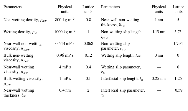
, where the subscripts p and l denote physical and lattice quantities, respectively. From the single-pore validation illustrated in figure 4, the slip and heterogeneous viscosity parameters required for pore-scale simulations are quantitatively identified. These parameters, calibrated at the single-pore level, are subsequently employed to simulate two-phase flow in more complex porous media. The corresponding physical and lattice parameters used in this study are summarised in table 1. The calibration procedure is based on MD simulations of n-alkane–water systems in quartz nanopores, which are representative of hydrophilic tight sandstone and shale oil reservoirs. As these parameters are directly constrained by molecular-scale velocity profiles, they ensure physical consistency and numerical reliability in pore-scale LB simulations. Nevertheless, the proposed workflow is general and can be readily extended to other mineral systems by incorporating the corresponding MD data.
Parameters used in LB simulations.

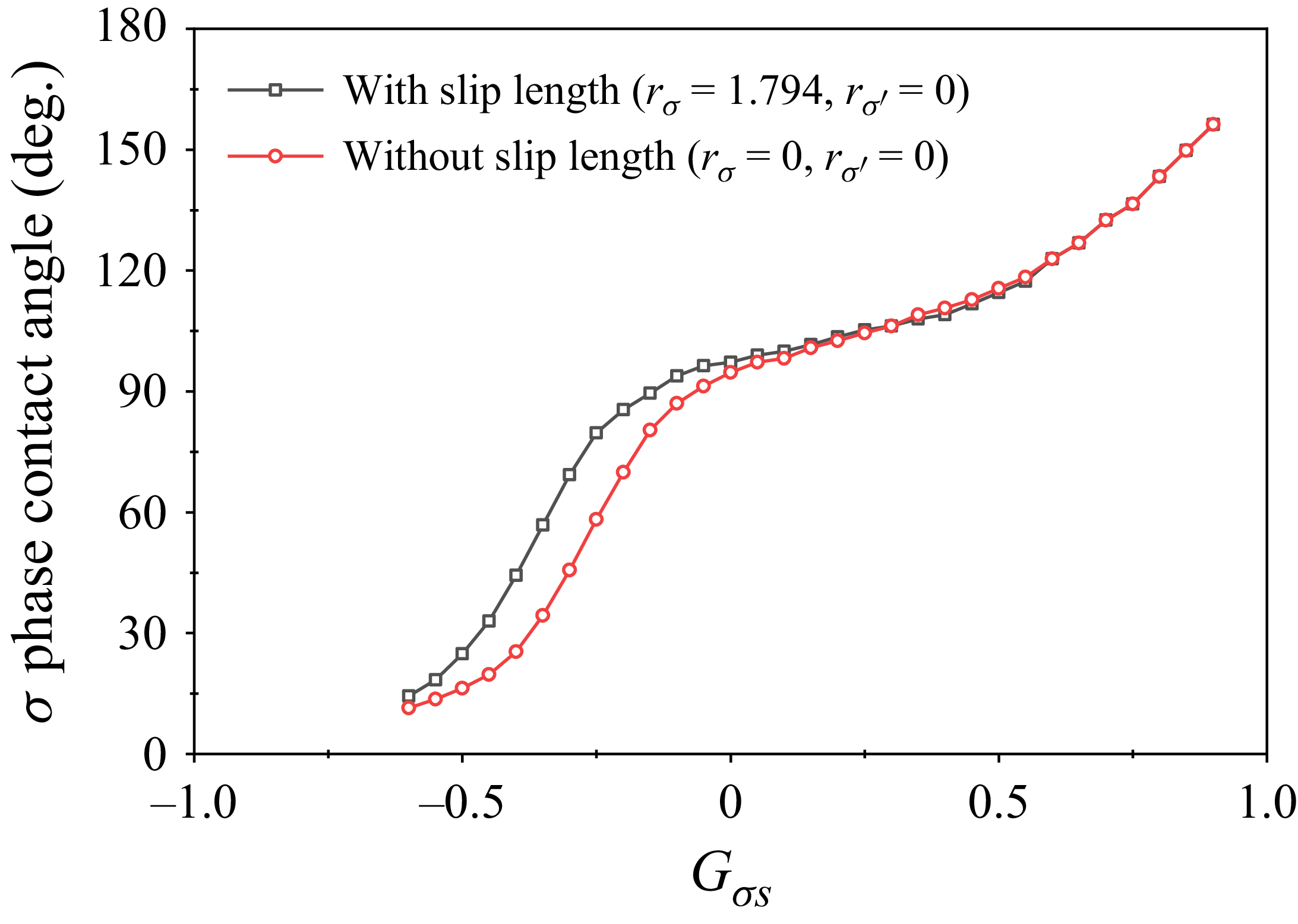
The wetting contact angle is a key parameter for accurately modelling two-phase flow. Within the pseudopotential LB framework, different contact angles can be realised by tuning the fluid–solid interaction parameter in (2.13). The implementation of slip boundary conditions modifies the wall-adjacent unknown distribution functions after streaming, thereby influencing the relationship between the fluid–solid interaction parameter and the resulting equilibrium contact angle. Figure 5 illustrates the dependence of the wetting contact angle on the fluid–solid interaction parameter
 $G_{\sigma s}$
, with and without the consideration of slip boundaries. The results indicate that the model can flexibly reproduce different wetting conditions.
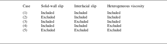
Summary of simulation cases.

Contact angle of
 $\sigma$
phase as a function of the fluid–solid interaction parameter
 $G_{\sigma s}$
.

4. Numerical results and discussion
4.1. Effect of molecular interactions
To better understand the flow mechanisms under nanoconfinement, it is essential to account for the influence of molecular interactions on fluid transport. These interactions induce three key physical nanoscale effects in multiphase systems, namely solid-wall slip, two-phase interfacial slip and heterogeneous viscosity. Each of these effects may significantly alter the flow behaviour of the wetting and non-wetting phases in nanoconfined porous media. As summarised in table 2, five simulation cases are designed to systematically isolate and evaluate the impact of these effects. Case (1) includes all effects, case (2) excludes solid-wall slip, case (3) excludes two-phase interfacial slip, case (4) excludes heterogeneous viscosity and case (5) excludes all three effects. These cases enable a systematic investigation into the role of each mechanism in phase displacement and provide insights into the dominant factors governing flow behaviours at the nanoscale.
Evolution of two-phase distribution and velocity fields in nanoporous media at different injected lattice times. (a) Evolution of two-phase distribution, where red and blue denote the non-wetting and wetting phases. (b) Velocity fields.
 $\theta _{w}=47^{\mathrm{o}} , \theta _{nw}=133^{\mathrm{o}} , S_{w}=0$
and
 $ \textit{Ca}=1.6\times 10^{-4}$
.

Regarding the overall displacement process, figure 6(a) clearly illustrates that the wetting phase preferentially flows through larger and well-connected pore-throat pathways, forming dominant flow channels. Early breakthrough along these dominant channels leaves large volumes of the non-wetting phase trapped in the pores on both sides of the channels. Nevertheless, the development of dominant channels significantly increases the interfacial contact area between the wetting phase, the solid matrix and the non-wetting phase, thereby promoting longitudinal spontaneous imbibition. Driven by capillary forces, the wetting phase subsequently invades pore spaces on both sides of dominant channels, which further enhances the overall displacement efficiency. Despite this enhanced displacement, part of the non-wetting phase remains trapped within the pore structure. This residual trapping primarily arises from two mechanisms. First, partially closed or poorly connected pore geometries restrict the mobility of the non-wetting phase. Second, capillary resistance leads to stable trapping configurations. The persistence of residual non-wetting phase reflects the combined effects of complex pore geometry and wettability characteristics of the nanoporous media and cannot be eliminated simply by increasing the external driving force. Localised magnified views in figure 7 illustrate the detailed mechanisms of capillary trapping. Figure 7(a) shows the distribution of the wetting and non-wetting phases in the pore1 and pore2 regions of the nanoporous media, while figure 7(b) presents the corresponding pressure fields calculated using (2.20). In these pore spaces, the non-wetting phase exists stably as fluid bridges between wetting phases, exhibiting typical capillary trapping behaviour. In some pores, the wetting phase imbibes along preferential pathways with an imbibition direction opposite to the overall displacement direction. As a result, the non-wetting phase is subjected to capillary forces acting from both ends. Taking the pore1 region as an example, the non-wetting phase is confined between two wetting phases, with a capillary pressure difference of P c1 = 0.004 at the left end and an opposing capillary pressure P c2 = 0.005 at the right end. Considering the displacement direction, the external driving force together with P c1 tends to mobilise the non-wetting phase, while P c2 acts as resistance. The dynamic balance between these competing forces significantly reduces the net driving force, rendering the non-wetting phase difficult to mobilise further and ultimately resulting in residual trapping.
Distributions of two phases (a) and pressure (b) in nanoporous media and pore structures at t = 2 000 000 lt. Here,
 $\theta _{w}=47^{\mathrm{o}} , \theta _{nw}=133^{\mathrm{o}} , S_{w}=0$
and
 $ \textit{Ca}=1.6\times 10^{-4}$
.

Difference maps of the non-wetting-phase distribution under different nanoscale effects. (a) Two-phase distributions with all nanoscale effects included. (b) Difference maps between considering all effects and no wall slip, and ΔD = D(excluding wall slip) − D(considering all effects). (c) Difference maps between considering all nanoscale effects and no interfacial slip, and ΔD = D(excluding interfacial slip) − D(considering all effects). (d) Difference maps between considering all effects and no heterogeneous viscosity, and ΔD = D(excluding heterogeneous viscosity) − D(considering all effects). (e) Difference maps between considering all and no nanoscale effects, and ΔD = D(considering no effects) − D(considering all effects). Here,
 $\theta _{w}=47^{\mathrm{o}} , \theta _{nw}=133^{\mathrm{o}} , S_{w}=0$
and
 $ \textit{Ca}=1.6\times 10^{-4}$
.

To evaluate the impact of molecular interactions on multiphase displacement, difference maps are constructed as ΔD = D (excluding a specific nanoscale effect) − D (considering all nanoscale effects), where D denotes the local non-wetting-phase distribution. As shown in figure 8, these difference maps highlight spatial regions where the flow behaviour is significantly influenced by each individual nanoscale mechanism. The displacement efficiency is defined as the ratio of the area of the displaced non-wetting phase to its initial area. In this section, the enhancement factor is defined as the ratio of the displacement efficiency obtained with specific nanoscale effects included to that obtained in the baseline case without any nanoscale effects, thereby providing a quantitative measure of the contribution of nanoscale effects to the overall displacement performance. In addition, figure 9 illustrates the temporal evolution of displacement efficiency and enhancement factor under different nanoscale conditions.
Variation of displacement efficiency (a) and enhancement factor (b) with time and nanoscale effects. Here,
 $\theta _{w}=47^{\mathrm{o}} , \theta _{nw}=133^{\mathrm{o}} , S_{w}=0$
and
 $ \textit{Ca}=1.6\times 10^{-4}$
.

When all nanoscale effects are included, the two-phase distributions at t = 500 000 and t = 20 00 000 lt are shown in figure 8(a). The impact of neglecting a specific nanoscale effect is illustrated by the difference maps in figure 8(b–e). In these difference maps, red regions (ΔD > 0) denote non-wetting phase that remains undisplaced when specific nanoscale effect is ignored, while blue regions (ΔD < 0) indicate additional non-wetting phase that is displaced. As shown in figure 8(b), at t = 500 000 lt, the dominance of red over blue indicates a pronounced reduction in displacement efficiency when wall slip is neglected. As displacement proceeds, red regions progressively diminish while blue regions expand, suggesting that the influence of wall slip weakens with time. This trend is further confirmed in figure 9(b), which shows the temporal evolution of the enhancement factor under different nanoscale conditions. When wall slip is ignored, the enhancement factor remains consistently lower than that obtained with all nanoscale effects included, demonstrating that neglecting wall slip leads to reduced displacement efficiency. For interfacial slip, as illustrated by the red and blue regions in figure 8(c), relative motion between the wetting and non-wetting phases occurs during the displacement process. Interfacial slip at the fluid–fluid interface reduces interfacial resistance under such conditions, thereby enhancing displacement efficiency. This effect is most pronounced during the early stage of displacement, when extensive interfacial contact exists between the two phases. As displacement progresses, the interfacial area associated with relative flow decreases, leading to a weakened influence of interfacial slip. Consistently, figure 9(b) shows that neglecting interfacial slip results in a reduced enhancement factor in the early stage, which gradually approaches that obtained with all nanoscale effects included in the later stage.
Regarding heterogeneous viscosity, the near-wall viscosity of the wetting phase is higher than its bulk viscosity, which weakens flow, while the non-wetting phase exhibits a lower near-wall viscosity than its bulk viscosity, thereby enhancing flow (Wu et al. Reference Wu, Chen, Li, Li, Xu and Dong2017). As shown in figure 9(b), at the early stage of displacement, the enhancement factor obtained without considering heterogeneous viscosity is lower than that obtained with all nanoscale effects included, indicating that neglecting heterogeneous viscosity reduces displacement efficiency. This behaviour arises because the porous media are initially almost entirely occupied by the non-wetting phase. According to table 1, the near-wall viscosity of the non-wetting phase is lower than its bulk viscosity, which can enhance flow, therefore, ignoring this low near-wall viscosity reduces the overall flow capacity and displacement efficiency. As the wetting phase invades, the near-wall viscosity of the wetting phase is higher than its bulk viscosity, which greatly weakens flow. Then, the positive effects associated with the low near-wall viscosity of the non-wetting phase become smaller than the negative effects of the high near-wall viscosity of the wetting phase. As a result, neglecting heterogeneous viscosity leads to a higher displacement efficiency and thus an increased enhancement factor. This behaviour is further evidenced by figure 8(d), where the blue regions dominate over the red regions in the difference maps at t = 500 000 and t = 2 000 000 lt, indicating enhanced displacement when heterogeneous viscosity is neglected. When all nanoscale effects are simultaneously neglected, the overall difference in two-phase distribution is depicted in figure 8(e), and the enhancement factor decreases from approximately 1.4 to about 0.9 over time, as illustrated in figure 9(b). The nanoscale effects exert a positive effect on displacement behaviour in the early stage but gradually turn into a negative effect in the later stage. At the early stage (t = 500 000 lt), the positive contributions from wall slip and the small near-wall viscosity of the non-wetting phase enhance displacement efficiency. The positive contributions are also clearly reflected in the velocity fields shown in figure 6(b), where relatively higher flow velocities are observed during the initial displacement stage. In contrast, at the later stage (t = 2 000 000 lt), the contributions of slip effects decrease as the non-wetting phase is progressively displaced. Meanwhile, the wetting phase, characterised by a higher near-wall viscosity and zero wall slip, becomes dominant near the solid surfaces. As a result, the overall flow resistance increases, causing a reduction in local velocities, as evidenced by the velocity fields in figure 6(b), and ultimately leading to a net decrease in displacement efficiency.
4.2. Initial wetting-phase saturation-dependent influence of molecular interactions
This section investigates the effects of four different initial wetting-phase saturations (
 $S_{w}$
) on displacement behaviour and analyses the coupled influence of
 $S_{w}$
and molecular interactions. The initial two-phase distributions corresponding to different
 $S_{w}$
are shown in figure 3. Figure 10(a–d) illustrates the dynamic evolution of the non-wetting-phase distribution, where the colour transition from blue to red represents the progression of invasion with time, and the white regions denote unrecovered residual non-wetting phase. For different
 $S_{w}$
, the wetting phase preferentially advances through the central dominant flow channels. As shown by the green regions in figures 10(a) and 10(b), at lower
 $S_{w}$
(0 and 0.1), longitudinal spontaneous imbibition is more pronounced, enabling the wetting phase to further invade the pore spaces adjacent to the dominant channels, thereby enhancing displacement efficiency. In contrast, as shown by the green regions in figures 10(c) and 10(d), when
 $S_{w}$
increases (0.2 and 0.3), the effectiveness of longitudinal imbibition is weakened, resulting in increased trapping of the non-wetting phase and higher residual saturation. Figures 10(e) and 10(f) show the difference maps of non-wetting-phase distributions at the same time, obtained by subtracting the results under
 $S_{w}=0.3$
from those under
 $S_{w}=0$
. After excluding the influence of the initial
 $S_{w}$
on the phase distribution, the red regions in the difference maps indicate that non-wetting-phase displacement is significantly weakened under higher
 $S_{w}$
. Figure 11(a) presents the temporal evolution of displacement efficiency under various
 $S_{w}$
. The results clearly demonstrate that displacement efficiency under
 $S_{w}=0.3$
is consistently lower than that under
 $S_{w}=0$
, indicating that a higher initial
 $S_{w}$
inhibits the effectiveness of wetting-phase displacement of the non-wetting phase.
Two-phase displacement process in nanoporous media at different times and
 $S_{w}$
conditions; (a)
 $S_{w}=0$
, (b)
 $S_{w}=0.1$
, (c)
 $S_{w}=0.2$
, (d)
 $S_{w}=0.3$
. (e) Difference maps of non-wetting-phase distributions between
 $S_{w}=0$
and
 $S_{w}=0.3$
at t = 500 000 lt, and ΔD = D(
 $S_{w}=0.3$
) − D(
 $S_{w}=0$
). (f) Difference maps of non-wetting-phase distributions between
 $S_{w}=0$
and
 $S_{w}=0.3$
at t = 2,000,000 lt, and ΔD = D(
 $S_{w}=0.3$
) − D(
 $S_{w}=0$
). Here,
 $\theta _{w}=47^{\mathrm{o}} , \theta _{nw}=133^{\mathrm{o}}$
and
 $ \textit{Ca}=1.6\times 10^{-4}$
.

Variation of displacement efficiency (a) and enhancement factor (b) with time and
 $S_{w}$
. Here,
 $\theta _{w}=47^{\mathrm{o}} , \theta _{nw}=133^{\mathrm{o}}$
and
 $ \textit{Ca}=1.6\times 10^{-4}$
.

Distributions of two phases (a) and pressure (b) in nanoporous media and representative pore structures at
 $S_{w}=0.3$
and t = 2 000 000 lt. Here,
 $\theta _{w}=47^{\mathrm{o}} , \theta _{nw}=133^{\mathrm{o}}$
and
 $ \textit{Ca}=1.6\times 10^{-4}$
.

To elucidate the underlying mechanisms governing the variation of displacement efficiency with initial
 $S_{w}$
, a pore-scale force analysis is performed based on the two-phase distributions and pressure fields within different pore structures. Figures 12(a) and 12(b) illustrate the phase distributions and pressure fields in the nanoporous media and representative pore structures, respectively. During displacement, the non-wetting phase exhibits typical capillary trapping in the form of fluid bridges, while the wetting phase forms multiple stable fluid bridges across pore throats, generating significant capillary pressure differences across their interfaces. When these fluid bridges are arranged in series and separated by non-wetting segments, they impose strong capillary resistance on the non-wetting phase, forming a microscopic capillary resistance chain. As evidenced by the pressure field in figure 12(b), distinct pressure jumps occur at the ends of the fluid bridges, indicating local capillary pressure accumulation. Such accumulation requires a relatively high threshold pressure for the non-wetting phase to redistribute or overcome the blockage. With increasing initial
 $S_{w}$
, the number of fluid bridges increases substantially, enlarging the capillary-resistance-dominated trapping regions and significantly reducing the flow capacity of the non-wetting phase. Consequently, the displacement efficiency decreases with increasing
 $S_{w}$
. Interestingly, only minor variations in displacement efficiency are observed between the initial
 $S_{w}$
values of 0 and 0.1, as shown in figure 11(a). As the
 $S_{w}$
increases from 0 to 0.1, a continuous wetting-phase film develops along the solid walls, enhancing two-phase flow capacity through interfacial slip effects. This film formation is strongly saturation-dependent, and within this low-saturation regime the wetting phase predominantly exists as thin films coating the pore walls in most pores, as evidenced by the initial two-phase distributions shown in figure 3(c). The presence of these film-like structures increases the positive contribution of interfacial slip to the displacement process. However, when the
 $S_{w}$
exceeds 0.1, the wetting-phase film transitions into discrete fluid bridges, introducing stronger capillary resistance and thereby reducing displacement efficiency and spontaneous imbibition effectiveness. It should be noted that in realistic three-dimensional nanoporous media, the formation of wetting films and the subsequent triggering of snap-off events are strictly controlled by pore geometry, aspect ratio, connectivity, surface roughness and related structural heterogeneities (Lei, Gong & Lu Reference Lei, Gong, Lu and Wang2024; Zheng, Qi & Gong Reference Zheng, Qi, Gong, Bian and Ju2024; Lei, Gong & Lu Reference Lei, Gong, Lu, Yang, Yang and Wang2025). Although the critical saturation (0.1 in this work) associated with the film-to-bridge transition may differ between two-dimensional and three-dimensional systems, the competition between film-assisted flow and capillary-induced trapping remains a fundamental mechanism governing multiphase displacement in nanoporous media.
The enhancement factor provides deeper insight into the influence of interfacial slip effects on two-phase flow behaviour under molecular interactions and varying
 $S_{w}$
. As shown in figure 11(b), the enhancement factor varies over time for different initial
 $S_{w}$
. With the exception of the case with
 $S_{w}=0.1$
, the enhancement factor remains consistently greater than 1 during the early stage of displacement, indicating that molecular interactions contribute positively to two-phase displacement. Owing to the negative effects of the molecular-interaction-induced higher near-wall viscosity of the wetting phase, the positive effects of molecular interactions on two-phase displacement progressively weaken as
 $S_{w}$
increases. At later stages, the enhancement factor gradually decreases below 1, and the negative effects of molecular interactions on two-phase displacement become increasingly pronounced with increasing
 $S_{w}$
. Figure 13 presents the difference maps of the non-wetting-phase distribution at t = 500 000 lt, where the red regions indicate areas in which the contribution of nanoscale effects is underestimated when such molecular interactions are excluded. For
 $S_{w}=0$
, the dominance of red regions indicates that ignoring molecular interactions underestimates displacement efficiency. In contrast, for
 $S_{w}=0.3$
, comparable red and blue regions are observed, suggesting that increasing
 $S_{w}$
reduces the influence of nanoscale effects on displacement efficiency. These observations are consistent with the temporal evolution of the enhancement factor shown in figure 11(b). Notably, in the case of
 $S_{w}=0.1$
, the enhancement factor gradually decreases with time but remains consistently greater than 1, indicating a sustained positive contribution of molecular interactions throughout the displacement process. This behaviour is consistent with the analysis in figure 11(a), where the wetting phase primarily forms film-like structures along the pore walls, and the resulting interfacial slip markedly enhances two-phase flow capacity. Consequently, at
 $S_{w}=0.1$
, the displacement efficiency deviates from the monotonic trend observed for the other
 $S_{w}$
(0, 0.2 and 0.3).
Effect of molecular interactions on non-wetting-phase distributions under varying
 $S_{w}$
conditions at t = 500 000 lt. (a) Two-phase distributions considering all effects. (b) Difference maps of non-wetting-phase distributions between considering all and no nanoscale effects, and ΔD = D(considering no effects) − D(considering all effects). Here,
 $\theta _{w}=47^{\mathrm{o}} , \theta _{nw}=133^{\mathrm{o}}$
and
 $ \textit{Ca}=1.6\times 10^{-4}$
.

Two-phase displacement process in nanoporous media at different times and wetting-phase contact angles; (a)
 $\theta _{w}= 36^{\mathrm{o}}$
, (b)
 $\theta _{w}= 47^{\mathrm{o}}$
, (c)
 $\theta _{w}= 57^{\mathrm{o}}$
, (d)
 $\theta _{w}= 80^{\mathrm{o}}$
. (e) Difference maps of non-wetting-phase distributions between
 $\theta _{w}= 36^{\mathrm{o}}$
and
 $\theta _{w}= 80^{\mathrm{o}}$
at t = 500 000 lt, and ΔD = D(
 $\theta _{w}= 80^{\mathrm{o}}$
) − D(
 $\theta _{w}= 36^{\mathrm{o}}$
). (f) Difference maps of non-wetting-phase distributions between
 $\theta _{w}= 36^{\mathrm{o}}$
and
 $\theta _{w}= 80^{\mathrm{o}}$
at t = 2 000 000 lt, and ΔD = D(
 $\theta _{w}= 80^{\mathrm{o}}$
) − D(
 $\theta _{w}= 36^{\mathrm{o}}$
). Here,
 $\theta _{nw}=180^{\mathrm{o}}-\theta _{w} , S_{w}=0.1$
and
 $ \textit{Ca}=1.6\times 10^{-4}$
.

4.3. Wettability-dependent influence of molecular interactions
Displacement simulations under four different wettability conditions are conducted for initial
 $S_{w}$
of 0.1 and 0.3, and the coupled influence of wettability and molecular interactions is analysed. Figure 14(a–d) illustrates the dynamic displacement processes under varying wetting-phase contact angles. In all cases, the wetting phase preferentially flows through the central dominant channels during the early stage of displacement. At later stages, smaller wetting-phase contact angles correspond to stronger capillary forces, which facilitate longitudinal spontaneous imbibition of the wetting phase into surrounding pores, enhancing displacement efficiency. Figures 14(e) and 14(f) present difference maps of non-wetting-phase distributions at the same time step, obtained by subtracting the non-wetting-phase distributions at a contact angle of 36° from that at 80°. The dominance of red regions in the difference maps indicates that larger wetting-phase contact angles are associated with reduced displacement efficiency. Figure 15(a) shows the temporal evolution of displacement efficiency under different wettability conditions and
 $S_{w}=0.1$
. The displacement efficiency at a contact angle of 80° is significantly lower than that at 36°. To elucidate this difference, figures 16(a) and 16(b) present the two-phase distributions and pressure fields at t = 500 000 lt, respectively, while representative pore structures with their corresponding distributions are further analysed in figures 16(c) and 16(d). At a contact angle of 36°, the meniscus curvature indicates that the capillary force acts along the flow direction, serving as an additional driving force for displacement. In contrast, at a contact angle of 80°, the capillary force opposes the displacement direction and thus acts as a resistance. Under the same displacement pressure, the presence of capillary driving force promotes spontaneous imbibition, whereas capillary resistance hinders fluid flow and reduces displacement efficiency. It is noteworthy that the displacement efficiency does not change significantly when the contact angle increases from 36° to 57°. Within this range, the capillary force remains favourable for flow, allowing the wetting phase to spontaneously enter small pores. Meanwhile, the wetting phase develops stable spreading films along the pore walls, which enhance interfacial slip and contribute positively to the displacement process. However, when the contact angle increases to 80°, the meniscus morphology reveals that the capillary force becomes resistive. Under this condition, the wetting phase tends to exist in droplet-like configurations on the pore walls and forms fluid bridges in narrow pores, significantly increasing flow resistance and leading to a marked decline in displacement efficiency. Figure 15(c) shows the temporal evolution of displacement efficiency under different wettability conditions and
 $S_{w}=0.3$
, and indicates that wettability exerts a limited influence on the final displacement efficiency. The primary reason is that, at higher wetting-phase saturation, numerous wetting-phase bridge structures form within the nanoporous media. These bridge structures generate significant capillary resistance, which counteracts the capillary driving force associated with lower wetting-phase contact angles, thereby diminishing the positive effect of wettability on displacement efficiency.
Variation of displacement efficiency and enhancement factor with time and wetting-phase contact angle. (a) Displacement efficiency with
 $S_{w}=0.1$
. (b) Enhancement factor with
 $S_{w}=0.1$
. (c) Displacement efficiency with
 $S_{w}=0.3$
. (d) Enhancement factor with
 $S_{w}=0.3$
.
 $\theta _{nw}=180^{\mathrm{o}}-\theta _{w}$
and
 $ \textit{Ca}=1.6\times 10^{-4}$
.

Distributions of two phases and pressure in nanoporous media and pore structures under varying wetting-phase contact angles at t = 500 000 lt. (a) Two-phase distributions considering all effects in nanoporous media. (b) Distributions of pressure in nanoporous media. (c) Two-phase distributions considering all effects in pore structure. (d) Distributions of pressure in pore structure. (e) Difference maps of non-wetting-phase distributions between considering all and no nanoscale effects in nanoporous media, and ΔD = D(considering no effects) − D(considering all effects). Here,
 $\theta _{nw}=180^{\mathrm{o}}-\theta _{w} , S_{w}=0.1$
and
 $ \textit{Ca}=1.6\times 10^{-4}$
.

Figures 15(b) and 15(d) show the temporal evolution of the enhancement factor as a function of time under varying wettability conditions for initial
 $S_{w}$
values of 0.1 and 0.3. Figure 16(e) further illustrates the difference maps of non-wetting-phase distributions under two contact angles, with and without nanoscale effects, at
 $S_{w}=0.1$
. The red regions indicate areas where the contribution of nanoscale effects is underestimated when such molecular interactions are excluded, which is consistent with the interfacial slip-induced enhancement discussed in § 2. The influence of wettability on the enhancement factor appears limited, primarily because contact angle does not directly control the key nanoscale effects. However, wettability is inherently governed by fluid–solid molecular interactions. Wu et al. (Reference Wu, Chen, Li, Li, Xu and Dong2017)) developed a correlation based on molecular simulations and experimental data, demonstrating that a larger vacuum water contact angle corresponds to lower near-wall viscosity and greater wall slip. Despite this, a continuous quantitative relationship between two-phase contact angle and nanoscale effects remains underexplored, largely due to the lack of systematic molecular simulations or experimental measurements. Accordingly, the present study does not explicitly incorporate a direct coupling between contact angle and nanoscale effects. Instead, the analysis is based on fitted results derived from molecular simulations under specific mineral pore conditions. This limitation may partly account for the relatively weak sensitivity of the enhancement factor to contact angle variations observed in this study.
Two-phase displacement process in nanoporous media at different times and Ca; (a)
 $ \textit{Ca}=4.2\times 10^{-5}$
, (b)
 $ \textit{Ca}=8.1\times 10^{-5}$
, (c)
 $ \textit{Ca}=1.6\times 10^{-4}$
, (d)
 $ \textit{Ca}=2.4\times 10^{-4}$
. (e) Difference maps of non-wetting-phase distributions between
 $ \textit{Ca}=4.2\times 10^{-5}$
and
 $ \textit{Ca}=2.4\times 10^{-4}$
at t = 500 000 lt, and ΔD = D(
 $ \textit{Ca}=2.4\times 10^{-4}$
) − D(
 $ \textit{Ca}=4.2\times 10^{-5}$
). (f) Difference maps of non-wetting-phase distributions between
 $ \textit{Ca}=4.2\times 10^{-5}$
and
 $ \textit{Ca}=2.4\times 10^{-4}$
at t = 2 000 000 lt, and ΔD = D(
 $ \textit{Ca}=2.4\times 10^{-4}$
) − D(
 $ \textit{Ca}=4.2\times 10^{-5}$
). Here,
 $\theta _{w}=47^{\mathrm{o}} , \theta _{nw}=133^{\mathrm{o}}$
and
 $S_{w}=0.1$
.

4.4. Capillary number-dependent influence of molecular interactions
This section investigates the influence of Ca on the displacement behaviour of the wetting phase at initial
 $S_{w}$
values of 0.1 and 0.3, and analyses the coupled effects of Ca and molecular interactions. Figure 17(a–d) illustrates the time-evolving displacement behaviour of the wetting phase in nanoporous media at Ca values of 4.2 × 10⁻⁵, 8.1 × 10⁻⁵, 1.6 × 10⁻⁴ and 2.4 × 10⁻⁴, respectively. As Ca increases, the wetting phase demonstrates a significantly enhanced ability to advance along dominant channels, exhibiting a pronounced finger-like feature. In addition, longitudinal spontaneous imbibition becomes more evident at higher Ca, enabling deeper penetration of the wetting phase into the porous structure and thereby improving displacement efficiency. Figures 17(e) and 17(f) present difference maps of non-wetting-phase distributions between high- and low-Ca cases, obtained by subtracting the low-Ca results from the high-Ca results. Blue regions indicate areas where the non-wetting phase has been displaced under high Ca but remains trapped under low Ca. The dominance of blue regions at both time steps demonstrates that higher Ca enhances the invasion of the wetting phase and promotes more effective removal of the non-wetting phase. Overall, an increasing capillary number enables the wetting phase to rapidly advance along dominant channels while simultaneously promoting longitudinal spontaneous imbibition. These dual mechanisms help overcome capillary resistance, reduce residual trapping of the non-wetting phase and significantly enhance overall displacement efficiency, as shown in figures 18(a) and 18(c).
Variation of displacement efficiency and enhancement factor with time and Ca. (a) Displacement efficiency with
 $S_{w}=0.1$
, (b) enhancement factor with
 $S_{w}=0.1$
, (c) displacement efficiency with
 $S_{w}=0.3$
, (d) enhancement factor with
 $S_{w}=0.3$
. Here,
 $\theta _{w}=47^{\mathrm{o}} , \theta _{nw}=133^{\mathrm{o}}$
.

The effect of molecular interactions is further examined in figures 18(b) and 18(d). These figures illustrate the temporal evolution of the enhancement factor for different Ca values. In addition, figure 19 presents the phase distributions and the corresponding difference maps obtained from simulations with and without nanoscale effects. The red regions in figure 19(b) indicate areas where the contribution of nanoscale effects is underestimated when such molecular interactions are excluded. At
 $S_{w}=0.1$
, the enhancement factor decreases over time for all Ca cases but remains greater than unity, indicating that nanoscale mechanisms, such as reduced near-wall viscosity of the non-wetting phase and interfacial slip, continue to exert a positive influence on flow. As Ca increases, the enhancement factor gradually decreases, suggesting that the positive influence of nanoscale effects becomes progressively weaker. The primary reason is that as the driving force becomes more dominant, the proportion of the wetting phase within the nanoporous media increases at the same displacement time. Consequently, the high near-wall viscosity of the wetting phase exerts a stronger negative effect on flow, thereby reducing the net positive contribution of nanoscale effects. When
 $S_{w}=0.3$
and
 $ \textit{Ca}=4.2\times 10^{-5}$
, as shown in figure 18(d), the enhancement factor remains consistently greater than unity. This is mainly because the non-wetting phase still dominates the pore space under these conditions, and its relatively low near-wall viscosity, together with interfacial slip, allows nanoscale effects to enhance flow. However, with further increases in Ca, the wetting-phase saturation continues to rise, and its high near-wall viscosity eventually causes nanoscale effects to shift from a positive to a negative influence. Overall, the Ca value governs the role of molecular interactions mainly by controlling the invasion rate and spatial occupation of the wetting phase within the nanoporous media.
Effect of molecular interactions on the non-wetting-phase distributions under varying Ca at t = 500 000 lt. (a) Two-phase distributions considering all nanoscale effects. (b) Difference maps of non-wetting-phase distributions between considering all and no nanoscale effects, and ΔD = D(considering no effects) − D(considering all effects). Here,
 $\theta _{w}=47^{\mathrm{o}} , \theta _{nw}=133^{\mathrm{o}}$
and
 $S_{w}=0.1$
.

4.5. Robustness of nanoscale effects across different nanoporous structures
While the above analyses elucidate the nanoscale effects under a representative SEM-based nanoporous media, it remains necessary to examine whether the identified physical mechanisms and trends are robust with respect to variations in porous geometry. To this end, this section extends the simulations to different nanoporous medium configurations and conducts comparative displacement analyses to assess the generality of the nanoscale effects and their influence on multiphase displacement behaviour.
Two-phase displacement process in different nanoporous media, and the variation of displacement efficiency and enhancement factor with time and porous structure. (a) Dynamic displacement processes. (b) Difference maps of non-wetting-phase distributions between considering all and no nanoscale effects, and ΔD = D(considering no effects) − D(considering all effects) at t = 500 000 lt. (c) Difference maps of non-wetting-phase distributions between considering all and no nanoscale effects, and ΔD = D(considering no effects) − D(considering all effects) at t = 1 200 000 lt. (d) Displacement efficiency. (e) Enhancement factor. Here,
 $\theta _{w}=47^{\mathrm{o}} , \theta _{nw}=133^{\mathrm{o}} , S_{w}=0$
and
 $ \textit{Ca}=8.1\times 10^{-5}$
.

Based on the three different nanoporous media shown in figure 2( g – i ), figure 20(a) presents the two-phase displacement patterns at representative times, while figures 20(b) and 20(c) show the difference maps of the wetting-phase distributions between simulations that consider all nanoscale effects and those that neglect them. These difference maps indicate that nanoscale effects, including wall slip, interfacial slip and heterogeneous viscosity, exert systematic influences that do not depend on a specific pore geometry. Instead, they consistently modify the local phase distribution and the overall displacement capacity during two-phase flow. The temporal evolutions of displacement efficiency and enhancement factor are shown in figures 20(d) and 20(e). For all nanoporous media, the displacement efficiency increases monotonically with time, whereas the enhancement factor gradually decreases. This trend primarily arises because, as the displacing phase advances, the positive contributions from wall slip and low near-wall viscosity of the non-wetting phase progressively weaken, while the negative effects associated with the zero wall slip and higher near-wall viscosity of the wetting phase become increasingly pronounced. This behaviour is consistent with the general trends identified in the preceding sections. Compared with the SEM-based nanoporous medium, a notable difference is observed in these idealised nanoporous media, where the enhancement factor remains greater than unity throughout the entire displacement process. This indicates that, at later stages of displacement, the negative impacts induced by the zero wall slip and high near-wall viscosity of the wetting phase are insufficient to offset the cumulative positive enhancement resulting from the wall slip and low near-wall viscosity of the non-wetting phase during the early displacement stage.
Based on figures 11(b), 15(b), 15(d), 18(b), 18(d) and 20(e), an interesting phenomenon can be observed during the late stage of the displacement process. Under certain conditions, the enhancement factor exhibits a gradual increasing trend, indicating that, compared with simulations in which nanoscale effects are neglected, the displacement efficiency continues to improve when these nanoscale effects are taken into account. This behaviour can be attributed to two complementary mechanisms. First, when nanoscale effects are considered, wall slip and the reduced near-wall viscosity significantly decrease the flow resistance acting on the residual non-wetting phase, enabling its progressive mobilisation given sufficient time. In contrast, in similar pore regions where nanoscale effects are ignored, the residual non-wetting phase experiences much higher flow resistance and therefore remains largely immobile. Second, when nanoscale effects are neglected, the non-wetting phase is nearly completely displaced during the late stage, and the displacement efficiency approaches a plateau with only minor variations. By contrast, when nanoscale effects are considered, a non-negligible amount of residual non-wetting phase remains within the pore space. As the displacement proceeds, this non-wetting phase can be gradually mobilised and displaced, leading to a more pronounced late-stage improvement in displacement efficiency. Consequently, the enhancement factor may continue to increase under certain conditions.
In brief, these results demonstrate that the competition among wall slip, interfacial slip and heterogeneous viscosity, as well as the resulting evolution of displacement efficiency, is robust across different nanoporous media. Although the magnitude of the enhancement factor and its rate of decay may vary with pore structure, the underlying physical mechanisms and overall trends remain consistent, supporting the general applicability of the conclusions drawn in this study.
4.6. Universal scaling behaviour
Overall, the influence of nanoscale effects on multiphase displacement arises from the competition among wall slip, interfacial slip and heterogeneous viscosity. These dynamic effects are strongly regulated by the spatial distribution and relative saturation of the phases within nanoporous media. Figure 21 reveals a universal scaling relationship of the flow enhancement factor versus displacement efficiency across varying initial wetting-phase saturations, wettability conditions and capillary numbers, exhibiting a clear monotonic decreasing trend. At the early stage of displacement, the non-wetting phase occupies most of the pore space and maintains extensive contact with the solid walls. Under these conditions, wall slip of the non-wetting phase, together with its relatively low near-wall viscosity and the presence of interfacial slip, effectively reduces flow resistance, resulting in an enhancement factor remaining well above unity. As displacement proceeds and efficiency increases, the wetting phase progressively accumulates in the near-wall region. Owing to its zero wall slip and higher near-wall viscosity, viscous dissipation near the pore walls increases significantly. Consequently, the enhancement factor decreases steadily and may even fall below unity, indicating a net negative contribution from nanoscale effects. Importantly, despite the diversity of initial saturation conditions, wettability and capillary numbers, the critical displacement efficiency at which nanoscale effects transition from a positive to a negative contribution is consistently observed within a narrow range of approximately 0.4–0.6, indicating a robust and universal scaling behaviour.
Universal scaling of the flow enhancement factor against displacement efficiency across varying initial wetting-phase saturations, wettability conditions and capillary numbers.

The nanoscale LB framework offers important implications for engineering practice by explicitly resolving how molecular interactions govern multiphase displacement under strong confinement. The identification of wall slip, interfacial slip and heterogeneous viscosity as competing mechanisms provides a clear physical basis for understanding the non-Darcy flow behaviours frequently observed in unconventional reservoirs. Post-fracturing flow in unconventional reservoirs involves complex interactions among injected fluids, physicochemical additives and rock surfaces, which lead to dynamic variations in wettability, interfacial tension and capillary-driven imbibition processes (Minakov et al. Reference Minakov, Pryazhnikov, Neverov, Sukhodaev and Zhigarev2024). The present framework can be naturally extended to incorporate such physicochemical induced wettability and interfacial effects, thereby offering a mechanistic tool for investigating complicated multiphase transport in nanoscale pore–fracture structures with evolving physicochemical properties. With appropriate modifications, such as coupling heterogeneous viscosity with the driving force, the model can be employed to investigate the characteristic threshold pressure gradient phenomena commonly observed in unconventional reservoirs. Real reservoirs typically exhibit more complex mineral distributions, pore structures and liquid–liquid–gas coexistence, where competitive adsorption between different fluids may occur (Wang et al. Reference Wang, Zhang, Xia, Tian, Qin and Cai2024a , Reference Wang, Xia, Zhao, Wang and Cai2025b ), further complicating the influence of nanoscale effects on multiphase flow. The results of this study therefore provide a fundamental basis for understanding these mechanisms in realistic reservoir systems. Moreover, the proposed methodology enables the exploration of extreme but physically meaningful scenarios, including highly non-wetting or strongly wetting surfaces and strongly confined flows dominated by molecular interactions. Although such conditions are rarely encountered directly in engineering field-scale developments, they are valuable for revealing the limiting behaviour of confined multiphase transport and for establishing physical bounds on displacement efficiency and phase trapping. Beyond subsurface energy applications, the modelling framework and physical insights developed in this work are also applicable to a broad range of micro- and nanoscale transport problems, including environmental remediation and water purification, micro-nano-fluidic systems and energy conversion and storage.
5. Concluding remarks
Multiphase flow in nanoporous media is strongly influenced by fluid–fluid and fluid–solid molecular interactions that give rise to nanoscale effects such as wall slip, interfacial slip and heterogeneous viscosity. These nanoscale effects lead to significant deviations from Darcy-type flow behaviours, rendering existing pore-scale simulation methods insufficient to capture these effects. To address this gap, a nanoscale LB model incorporating molecular interactions is developed to investigate multiphase displacement in nanoporous media. The velocity profiles of single-phase and two-phase flow in single nanopores are first analysed and characterised using theoretical solutions based on the HP equation. A multiphase pseudopotential LB model is then developed, in which wall slip for both phases is implemented using a combined half-way bounce-back and diffusive slip boundary condition, interfacial slip is captured by dynamically tracking the fluid–fluid interface and accounting for the apparent viscosity within the interfacial region, and heterogeneous viscosity is incorporated by assigning different relaxation times to the near-wall and bulk fluids. The accuracy of the proposed model is then verified against molecular simulations and theoretical velocity profiles, and essential pore-scale parameters for the displacement simulations in nanoporous media are obtained through velocity fitting in single nanopores.
The nanoscale LB model is applied to simulate the displacement of the non-wetting phase by the wetting phase in nanoporous media, and to examine the effects of molecular interactions, initial wetting-phase saturation, wettability and capillary number on displacement behaviour. The influences of these factors on displacement patterns, displacement efficiency and phase trapping are analysed in detail based on phase and pressure distributions. Furthermore, the coupled effects of initial wetting-phase saturation, wettability and capillary number on molecular interaction-induced displacement patterns, efficiency and phase trapping are analysed. (i) Molecular interactions initially enhance displacement through wall slip and the low near-wall viscosity of the non-wetting phase. As displacement proceeds, diminishing wall slip and the increasing near-wall viscosity of the wetting phase lead to a gradual transition toward a negative contribution. (ii) At low wetting-phase saturation, a continuous wetting-phase film forms along pore walls, enhancing interfacial slip and significantly improving displacement efficiency. With increasing saturation, the development of wetting-phase bridges introduces capillary resistance that offsets or reverses the positive effects of molecular interactions. (iii) Smaller wetting-phase contact angles (≤57°) enhance displacement efficiency through capillary-driven spontaneous imbibition, whereas larger angles (≈80°) form droplet and bridge structures that raise flow resistance and reduce efficiency. (iv) With increasing capillary number, the invasion of the wetting phase grows, and the high near-wall viscosity of wetting phase progressively weakens the positive contribution of molecular interactions while strengthening their negative impact on displacement efficiency. In addition, displacement simulations in three idealised nanoporous media with distinct pore geometries exhibit consistent displacement efficiencies and nanoscale-induced behaviours, indicating that the above conclusions are robust and not limited to a specific porous structure. Moreover, a universal scaling relationship is observed between the flow enhancement factor and displacement efficiency across different flow conditions, with a consistent transition at a critical displacement efficiency of approximately 0.4–0.6, beyond which nanoscale effects change from enhancing to suppressing flow.
Overall, the influence of molecular interactions originates from wall slip, interfacial slip and heterogeneous viscosity associated with the wetting and non-wetting phases. Meanwhile, initial wetting-phase saturation, wettability and capillary number dynamically control the phase distributions and invasion behaviours, thereby balancing the negative contribution of the wetting phase, characterised by zero wall slip and higher near-wall viscosity, with the positive contribution of the non-wetting phase, associated with non-zero wall slip, lower near-wall viscosity and interfacial slip. These competing mechanisms collectively govern the net influence of molecular interactions on multiphase displacement in nanoporous media. The simulations are performed in two-dimensional nanoporous media, which cannot fully reproduce the pore connectivity, coordination number, and phase trapping mechanisms inherent to realistic three-dimensional nanoporous media. Consequently, the present findings are primarily intended for qualitative and mechanistic interpretation rather than direct quantitative upscaling to field-scale reservoir development.
Supplementary movies
Supplementary movies are available https://doi.org/10.1017/jfm.2026.11591.
Acknowledgements
Artificial intelligence tools are used to assist in polishing the language of the manuscript.
Funding
This study was supported by the National Natural Science Foundation of China (52404048, 52274056, 42172159), and Science Foundation of China University of Petroleum, Beijing (2462025YJRC027).
Declaration of competing interests
The authors declare that they have no known competing financial interests or personal relationships that could have appeared to influence the work reported in this paper.
Data availability statement
Data will be made available from the corresponding author on request.
Appendix A. Hagen–Poiseuille equation for single-phase flow in circular nanopores
The wall slip velocity can be determined from the slip length
 $l_{s}$
and the velocity gradient at the wall as follows:
 \begin{align} u_{s}=-l_{s}\left(\frac{\partial u_{n}}{\partial r}\right)| _{r={R_{1}}}=\frac{l_{s}{R}_{1}^{2}}{2\mu _{n}}\boldsymbol{\nabla }\!p . \end{align}
During fluid flow in nanopores, the velocity at the wall obtained from equation (2.1) equals the wall slip velocity from equation (A1). Moreover, the fluid velocity and shear stress are continuous across the near-wall and bulk regions. Therefore, the boundary conditions can be expressed as follows:
 \begin{align} -l_{s}\frac{\partial u_{n}}{\partial r}| _{r={R_{1}}}=u_{n}| _{r={R_{1}}} , \\[-28pt] \nonumber \end{align}
 \begin{align} u_{n}| _{r=\left(R_{1}-\delta _{1}\right)}=u_{b}| _{r=\left(R_{1}-\delta _{1}\right)} , \\[-28pt] \nonumber \end{align}
 \begin{align} \mu _{n}\frac{\partial u_{n}}{\partial r}| _{r=\left(R_{1}-\delta _{1}\right)}=\mu _{b}\frac{\partial u_{b}}{\partial r}| _{r=\left(R_{1}-\delta _{1}\right)} , \\[-28pt] \nonumber \end{align}
 \begin{align} \frac{\partial u_{b}}{\partial r}| _{r=0}=0 . \\[10pt] \nonumber \end{align}
Based on the boundary conditions of equations (A2)–(A5), together with the velocities given by equations (2.1) and (2.2), the coefficients
 $C_{1}$
and
 $C_{2}$
can be determined. Consequently, the velocities for the near-wall and bulk regions of single-phase flow in a single nanopore can be rewritten as
 \begin{align} u_{n}(y)=\left(\frac{{R}_{1}^{2}-r^{2}}{4\mu _{n}}+\frac{l_{s}R_{1}}{2\mu _{n}}\right)\boldsymbol{\nabla }\!p, R_{1}-\delta _{1}\leq r\leq R_{1} , \\[-28pt] \nonumber \end{align}
 \begin{align} u_{b}=\left(\frac{\left({R}_{1}^{2}-r^{2}\right)}{4\mu _{b}}+\left(\frac{\left({R}_{1}^{2}-\left(R_{1}-\delta _{1}\right)^{2}\right)}{4\mu _{n}}-\frac{\left({R}_{1}^{2}-\left(R_{1}-\delta _{1}\right)^{2}\right)}{4\mu _{b}}+\frac{l_{s}R_{1}}{2\mu _{n}}\right)\right)\boldsymbol{\nabla }\!p,0\leq r\leq R_{1}-\delta _{1} . \\[0pt] \nonumber \end{align}
Appendix B. Hagen–Poiseuille equation for two-phase flow in circular nanopores
During two-phase flow in nanopores, the wall velocity satisfies the Navier slip condition given by equation (B1). Moreover, the fluid velocity and shear stress are continuous across the regions of near-wall wetting phase, bulk wetting phase, interfacial phase and bulk non-wetting phase. Therefore, the boundary conditions can be expressed as follows:
 \begin{align} -l_{s}\frac{\partial u_{nw}}{\partial r}| _{r={R_{1}}}=u_{nw}| _{r={R_{1}}} , \\[-28pt] \nonumber \end{align}
 \begin{align} u_{nw}| _{r=({R_{1}}-{\delta _{1}})}=u_{bw}| _{r=({R_{1}}-{\delta _{1}})} , \\[-28pt] \nonumber \end{align}
 \begin{align} \mu _{nw}\frac{\partial u_{nw}}{\partial r}| _{r=({R_{1}}-{\delta _{1}})}=\mu _{bw}\frac{\partial u_{bw}}{\partial r}| _{r=({R_{1}}-{\delta _{1}})} , \\[-28pt] \nonumber \end{align}
 \begin{align} u_{bw}| _{r={R_{2}}}=u_{i}| _{r={R_{2}}} , \\[-28pt] \nonumber \end{align}
 \begin{align} \mu _{bw}\frac{\partial u_{bw}}{\partial r}| _{r={R_{2}}}=\mu _{i}\frac{\partial u_{i}}{\partial r}| _{r={R_{2}}} , \\[-28pt] \nonumber \end{align}
 \begin{align} u_{i}| _{r=({R_{2}}-{\delta _{2}})}=u_{bnw}| _{r=({R_{2}}-{\delta _{2}})} , \\[-28pt] \nonumber \end{align}
 \begin{align} \mu _{i}\frac{\partial u_{i}}{\partial r}| _{r=({R_{2}}-{\delta _{2}})}=\mu _{bnw}\frac{\partial u_{bnw}}{\partial r}| _{r=({R_{2}}-{\delta _{2}})} , \\[-28pt] \nonumber \end{align}
 \begin{align} \frac{\partial u_{bnw}}{\partial r}| _{r=0}=0 . \\[0pt] \nonumber \end{align}
Based on the boundary conditions of equations (B1)–(B8), together with the velocities given by equations (2.3)–(2.6), the coefficients
 $C_{3} , C_{4} , C_{5} , C_{6}$
can be determined. Consequently, the velocities for two-phase flow in a single nanopore can be rewritten as
 \begin{align} u_{nw}(r)=\left(\frac{{R}_{1}^{2}-r^{2}}{4\mu _{nw}}+l_{s}\frac{R_{1}}{2\mu _{nw}}\right)\boldsymbol{\nabla }\!p, \left(R_{1}-\delta _{1}\right)\lt r\leq R_{1} , \\[-28pt] \nonumber \end{align}
 \begin{align} u_{bw}(r)=\left(\frac{{R}_{1}^{2}-r^{2}}{4\mu _{bw}}+\frac{{R}_{1}^{2}-(R_{1}-\delta _{1})^{2}}{4\mu _{nw}}-\frac{{R}_{1}^{2}-(R_{1}-\delta _{1})^{2}}{4\mu _{bw}}+l_{s}\frac{R_{1}}{2\mu _{nw}}\right)\boldsymbol{\nabla }\!p, R_{2}\lt r\leq \left(R_{1}-\delta _{1}\right) , \\[-28pt] \nonumber \end{align}
 \begin{align} u_{i}(r)& =\left(\frac{{R}_{1}^{2}-r^{2}}{4\mu _{i}}+\frac{{R}_{1}^{2}-{R}_{2}^{2}}{4\mu _{bw}}-\frac{{R}_{1}^{2}-{R}_{2}^{2}}{4\mu _{i}}+\frac{{R}_{1}^{2}-(R_{1}-\delta _{1})^{2}}{4\mu _{nw}}\right. \nonumber \\ & \quad \left. -\frac{{R}_{1}^{2}-(R_{1}-\delta _{1})^{2}}{4\mu _{bw}}+l_{s}\frac{R_{1}}{2\mu _{nw}}\right)\boldsymbol{\nabla }\!p, \left(R_{2}-\delta _{2}\right)\lt r\leq R_{2} , \\[-28pt] \nonumber \end{align}
 \begin{align} u_{bnw}(r) & =\left(\frac{{R}_{1}^{2}-r^{2}}{4\mu _{bnw}}+\frac{{R}_{1}^{2}-(R_{2}-\delta _{2})^{2}}{4\mu _{i}}-\frac{{R}_{1}^{2}-(R_{2}-\delta _{2})^{2}}{4\mu _{bnw}} \right. \nonumber \\ & \quad \left. +\frac{{R}_{1}^{2}-{R}_{2}^{2}}{4\mu _{bw}}-\frac{{R}_{1}^{2}-{R}_{2}^{2}}{4\mu _{i}}+\frac{{R}_{1}^{2}-(R_{1}-\delta _{1})^{2}}{4\mu _{nw}}-\frac{{R}_{1}^{2}-(R_{1}-\delta _{1})^{2}}{4\mu _{bw}} \right. \nonumber \\ & \quad \left. +l_{s}\frac{R_{1}}{2\mu _{nw}}\right)\boldsymbol{\nabla }\!p,0\leq r\leq \left(R_{2}-\delta _{2}\right) . \\[0pt] \nonumber \end{align}
Appendix C. Equation for two-phase Poiseuille flow in slit nanopores
Assuming the geometry in figure 1(b) represents a two-dimensional slit pore, where
 $R_{1}$
denotes the half-width of the slit nanopore, the velocity equations for the two-phase Poiseuille flow can be expressed as follows:
 \begin{align} u_{nw}(y)=\frac{1}{2\mu _{nw}}\boldsymbol{\nabla }\!p\big({R}_{1}^{2}-y^{2}\big)+C_{7}, (R_{1}-\delta _{1})\lt y\leq R_{1} , \\[-28pt] \nonumber \end{align}
 \begin{align} u_{bw}(y)=\frac{1}{2\mu _{bw}}\boldsymbol{\nabla }\!p\big({R}_{1}^{2}-y^{2}\big)+C_{8}, R_{2}\lt y\leq (R_{1}-\delta _{1}) , \\[-28pt] \nonumber \end{align}
 \begin{align} u_{i}(y)=\frac{1}{2\mu _{i}}\boldsymbol{\nabla }\!p\big({R}_{1}^{2}-y^{2}\big)+C_{9}, (R_{2}-\delta _{2})\lt y\leq R_{2} , \\[-28pt] \nonumber \end{align}
 \begin{align} u_{bnw}(y)=\frac{1}{2\mu _{bnw}}\boldsymbol{\nabla }\!p\big({R}_{1}^{2}-y^{2}\big)+C_{10},0\leq y\leq (R_{2}-\delta _{2}) , \\[0pt] \nonumber \end{align}
where
 $C_{7} , C_{8} , C_{9} , C_{10}$
are coefficients related to the molecular interactions, which can be obtained from the interfacial and boundary continuity conditions. The same boundary conditions as those established for the circular pore (see (B1)–(B8)) are adopted here, including the Navier slip condition at the solid wall and the continuity of velocity and shear stress across different regions. Accordingly, these coefficients are directly obtained as
 \begin{align} C_{7}=l_{s}\frac{R_{1}}{\mu _{nw}}\boldsymbol{\nabla }\!p , \\[-28pt] \nonumber \end{align}
 \begin{align} C_{8}=\left(\frac{{R}_{1}^{2}-(R_{1}-\delta _{1})^{2}}{2\mu _{nw}}-\frac{{R}_{1}^{2}-(R_{1}-\delta _{1})^{2}}{2\mu _{bw}}\right)\boldsymbol{\nabla }\!p+C_{7} , \\[-28pt] \nonumber \end{align}
 \begin{align} C_{9}=\left(\frac{{R}_{1}^{2}-{R}_{2}^{2}}{2\mu _{bw}}-\frac{{R}_{1}^{2}-{R}_{2}^{2}}{2\mu _{i}}\right)\boldsymbol{\nabla }\!p+C_{8} , \\[-28pt] \nonumber \end{align}
 \begin{align} C_{10}=\left(\frac{{R}_{1}^{2}-(R_{2}-\delta _{2})^{2}}{2\mu _{i}}-\frac{{R}_{1}^{2}-(R_{2}-\delta _{2})^{2}}{2\mu _{bnw}}\right)\boldsymbol{\nabla }\!p+C_{9} . \\[0pt] \nonumber \end{align}