Since the publication of Robert W. Fogel and Stanley L. Engerman's Time on the Cross, economic historians have been actively debating the validity of one of their central propositions—that slaves were allowed, and encouraged, to maintain family ties because doing so enhanced the value of slaves to their owners. Laurence Kotlikoff investigated the potential effect of family connections on the value of slaves sold in the New Orleans market at the time of their sale.Footnote 1 If preserving family ties enhanced the value of slaves to their owners, as Fogel and Engerman posited, the value of slave family members sold together would be higher. Kotlikoff found that the value of mother-father-child groups—a rare event in the data—was higher than the combined value of the members of the family if they were sold singly. However, other family combinations, including mother-child sales—by far the most common form of family sale—suffered large discounts when compared to the sales of identical family members sold separately.
Fogel and Engerman argued that this finding could reflect a scale discount associated with slave sales—by selling the slaves as a group rather than singly, the sum of transactions costs would be reduced, or equivalently, buyers would realize a scale discount.Footnote 2 If the discount outweighed the economic benefits associated with family ties, family members would sell at a discount rather than a premium. If that explanation were correct, it could be confirmed by empirical analysis of two questions: (1) Is there a scale discount for selling slaves irrespective of whether they are family members or not; and (2) Do slave groups of any particular size command higher market prices when the members of the group sold are family members (as opposed to unrelated group members)? To our knowledge, no one has investigated these questions empirically.
A related issue is the need to consider the potential effect of selectivity bias in the slave sales process. Slaves who are sold are likely not a random sample of slaves in the population. In addition, it is possible that slave family members sold together are selected for sale through a different process than slaves sold individually. If that were true, then the family discount observed in the sales of slave family groups might reflect differences in the selection process for the sale of families compared to the selection process for the sale of individuals. If selectivity bias explains the family discount, then observed discounts may give a distorted measure of the underlying value (in the broader slave population) to masters of keeping slave families together.
Independent of their owners' economic interests, families would not exist without the active support and participation of the slaves themselves. The family served, among other things, as a form of long-term life insurance against the hardships of slavery. Owners sometimes may have benefited from this mutual dependency by selling family members together rather than singly. Most obviously, if one member of the group were weak or sick, that individual might be sold with another member of his family because the joint value of the two would be greater than their value if sold separately. This negative selection of family groups would produce a family discount, which is simply indicative of the lower market price attached to the weak, sick, or needy member of the family group.
Transport costs may have affected the average value of slaves shipped in family groups versus the value of slaves shipped singly. When a fixed transport cost is applied to two similar goods, the effect is to lower the relative price of the higher quality good. Because shipment of slaves was costly, the relative price of high-valued slaves was lower in New Orleans, and as a consequence, buyers preferred to purchase relatively more of them. Positive selection is likely to have its greatest effect on the attributes of children chosen for market—only the healthiest and most robust would justify the cost of shipment.Footnote 3 In deciding whether to ship a family to New Orleans, a trader would consider the attributes of the entire family, not just those of the children. It is possible that the children shipped with families were less rigorously selected than the children shipped singly. In addition, it might have been cheaper to ship a child with a parent rather than by himself. If that were true, then the selection produced by transport costs for the attributes of family members could be different from those of individuals.
Legal restrictions could also have played a role in producing observed price differences between family group members and stand-alone slaves. Children under the age of ten could not be legally sold alone unless they were orphans. Also, superannuates were legally required to be sold jointly with a child (if one were present). If these Louisiana laws were enforced, that may have reduced the market value of slaves sold as part of family groups.
We test these various explanations of group scale discounts, and family-ties premia or discounts, using prices for slaves sold in the New Orleans market from 1820 through 1860. We distinguish sales of groups that include family and nonfamily members, and family group sales of different types (those involving small children, and other sales), to investigate how family-ties premia or discounts vary with the structure of the family sold. Our results from slave price regressions lend support to the view that selectivity bias involving family groups, rather than economies of scale in selling, explains the observed group discounts.
Absent scale discounts, the fact that family groups sold at discount suggests that slave owners benefited from preserving families when those family members had relatively low stand-alone market values. Otherwise, in the absence of an economic benefit, sellers could have increased their profit by separating families at the time of sale. Stated differently, under the assumption of zero arbitrage profits, the fact that heavily discounted family group sales occurred provides evidence of selectivity bias, which reflected the voluntary provision of care among slave family members. Slave owners' decisions not to separate families despite a family discount indicated that they perceived that the sum of the stand-alone prices they would have received by separating families would have been lower than the discounted family group sale price, presumably because of the assistance and care that family members voluntarily provided one another.
In the case of family groups involving parent-child relationships, one can gauge the potential importance of selectivity bias by examining additional data. We examine data from ship manifests on the heights of slave children during their transport for sale to the New Orleans slave market. We find that children traveling as members of family groups are substantially shorter (by roughly two inches) than children of the same age and sex that we identify as traveling separately. We argue that the taller stature of children shipped without parents provides further evidence that some form of selectivity by traders explains the family-ties discounts observed in the New Orleans slave market. We find that transport costs resulted in higher values for imported slaves, but the size of group family discounts is unrelated to whether a slave is imported or not. We find some evidence for the role of legal restrictions in boosting family discounts (after legal changes in 1829), but legal factors cannot explain most of our findings.
MODELING SLAVE PRICES FROM NEW ORLEANS SALES
We use the New Orleans Slave Sale Sample, originally collected under the direction of Fogel and Engerman, and used previously by Kotlikoff, Bruce Greenwald and Robert Glasspiegel, Herman Freudenberger and Pritchett, and Eugene Choo and Jean Eid.Footnote 4 During the first part of the nineteenth century, New Orleans was the center of slave trading in the South. Transactions included both local slave sales and sales of imported slaves, often brought by ship from elsewhere in the South. Because of its French legal tradition, slaves in Louisiana were considered real estate rather than personal property, and as such, all slave sales had to be notarized.Footnote 5 The Fogel and Engerman slave sale sample was drawn from the New Orleans Notarial Archives, which was created in 1867 to serve as a depository of the notarial records. These records are not a complete set of transactions—some notarial records were destroyed in office fires, whereas others were simply lost. Depending on the year of sale, between 2.5 and 5 percent of the extant notarial records comprise the sample of slave sales recorded by Fogel and Engerman.
The sample contains 2,169 usable observations of stand-alone sales of slaves, which we define as transactions in which only one slave was sold. The data set also contains 683 usable group sale transactions. Recorded characteristics of the individuals in the group include their age, sex, and family relationship (although it is possible that family relationships were not always noted). Other data fields include information about the degree of skin darkness, whether the transaction was for cash or credit, and whether the slaves were sold with a guarantee.Footnote 6 Prices are normalized, as in Kotlikoff, by dividing the observed price by the average price of a male, aged 21 to 38 years, sold in that same year. This procedure avoids the need to control for price changes over time.Footnote 7
Before discussing our approach to modeling the factors that affected the pricing of slave groups, it is useful to review some of the differences between the samples of stand-alone and group transactions, and the frequency of different types of groups. Such information offers important hints about potential selectivity in the determination of whether a slave was included in a group or stand-alone transaction, or a particular type of group transaction.
Most obviously, the age distributions are very different for the stand-alone and group samples. The group sample includes more children, especially young ones. Children younger than ten represent 3 percent of stand-alones and nearly 29 percent of group sales. Legal restrictions may have reduced the number of children under the age of ten years sold without their parent. Additional legal restrictions applied to the separate sale of weak or sick slaves, who are more frequently elderly. In addition, differences in the age distributions may reflect different economic advantages from preserving familial relationships for slaves of different ages.
Relatively few intact families were sold in New Orleans and most family groups were comprised of mothers with children. Family group members accounted for 45 percent of the total number of slaves sold in groups. Most family group members (87 percent) consisted of mothers and their children, and the most common family group consisted of a mother with children (90 percent). Mother-father-child groups were rare (only 3.6 percent of the total number of family groups). Other adult family affiliations (by which we mean other family groupings in which children age 13 and younger were not present) took the form of husband-wife pairs and sibling groupings.
We construct a model of stand-alone slave sales to serve as our benchmark for group sales. The stand-alone model can be used to generate predicted values for each group sale by adding together the predicted values of each group member to create a composite predicted value for the group.Footnote 8 We then predict group discounts or premia, defined as the logarithm of the difference of the actual and predicted group price, using the characteristics of the group.
First, we estimate a stand-alone model that regresses observed stand-alone prices on a variety of slave characteristics. This model is a modification of Kotlikoff's pricing model, which includes the regressors listed in Table 1. The most important difference between our stand-alone model and Kotlikoff's model arises because we apply the Kotlikoff model only to stand-alone transactions. Kotlikoff included mother-child transactions in his model, while we model them separately in our group transactions analysis. In other respects, however, our model is very close to Kotlikoff's. We experimented with a variety of alternative specifications for the age-sex distribution and found that none of them substantially improved the fit of the stand-alone model. In response to a suggestion from Engerman, we added indicator variables that capture whether slave buyers or slaves were from New Orleans. We found that this addition improved the fit of both the stand-alone and group regression models, but does not affect other results.
Table 1 reports the estimation results for our stand-alone version of the Kotlikoff model. The results are familiar. Males are worth more. Light skin adds some market value for females, but not for males. Guarantees raise prices. Transactions that involve credit require higher prices. The effect of age is estimated by a six-order polynomial. The prices of men and women peak in their early 20s, and values drop dramatically in the late 30s and 40s. The residuals from the stand-alone regression are similar across the range of slave ages in the sample. In particular—and importantly for our discussion below of group sales regressions—the regression does not over predict the prices of stand-alone children or superannuates.
GROUP SALES REGRESSIONS
We turn now to the group sales regressions. The dependent variable is the “group premium,” defined as the logarithm of the difference between the actual group price and the sum of the predicted stand-alone prices for the group members, using the coefficients from Table 1 to generate predicted prices for each group member. We investigate the effects of several potential influences in producing predictable
NEW ORLEANS SLAVE PRICE STRUCTURE, INDIVIDUAL SALES REGRESSION COEFFICIENTS, MEANS, AND STANDARD DEVIATIONS

*indicates the regression coefficient is statistically different from zero at the 10 percent level.
Notes:
The dependent variable is the logarithm of the slave's price relative to the average annual price of a male slave, aged 21 to 38 years. Sample includes New Orleans slaves sold singly. The omitted variable refers to unguaranteed dark-colored females, without a reported skill, sold for cash in September. Standard errors are listed in parentheses beneath regression coefficients.
Source:
Fogel and Engerman, “New Orleans Slave.”
that larger groups have smaller error terms. We also ran regressions using heteroskedasticity correction to control for differences in errors across groups, and found very similar results. Also, ordinary least squares regressions (not reported here) are qualitatively very similar to the results in Table 2.
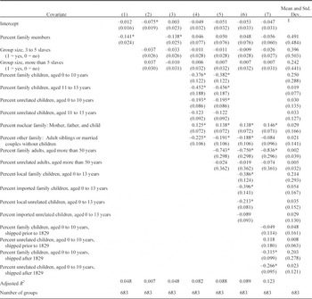
PERCENT GROUP PREMIUM, WEIGHTED LEAST SQUARES REGRESSION COEFFICIENTS

*indicates that the regression coefficient is statistically different from zero at the 10 percent level.
Notes:
The dependent variable equals the logarithm of the quotient of the actual and predicted group price, where the predicted group price equals the sum of the predicted prices for group members, derived from Table 1. Predicted prices are adjusted for the logarithm of the standard error. Observations are weighted by group size. The omitted variable represents a group size of two slaves. The sample includes group sales (of more than one slave), excluding groups with a missing value for the age of an individual. Standard errors are listed in parentheses beneath regression coefficients.
Source:
Fogel and Engerman, “New Orleans Slave.”
Scale and Group Discounts
Fogel and Engerman hypothesized that the size of the group sold may lead to differences in pricing if larger transactions enjoy scale discounts.Footnote 9 We investigate this hypothesis by dividing our group sample into three groups by size: groups of two people, groups of three-five people, and groups of more than five people. Finer divisions of the sample, or alternative specifications of size effects yield similar results to those reported in Table 2 and are not reported here.
Equation 2, located in Table 2, provides the simplest version of a regression testing for scale effects in the group premium. Groups of two people are contained in the intercept, and indicator variables are included for group sizes of three to five and over five. The three coefficient estimates indicate that statistically significant group discounts averaging 7.5 percent are present for groups of two people; for groups of three-five people, discounts average 11.2 percent and are statistically significant; and groups of more than five people display a 3.8 percent average discount, which is not statistically different from zero at the 10 percent significance level. Equation 2, therefore, suggests the opposite of a scale discount for group sales, since larger groups command a lower discount.
Once one controls for the family and age structure of groups, the scale premium observed in equation 2 disappears. Equation 3 adds the percentage of group members that are related as family members to the group size indicators, and equations 4 and 5 add variables that capture the structure of family and nonfamily groups.Footnote 10 When these variables are added, the intercept and the two group size indicator variables become small and are no longer statistically significant.
Families, Group Structure, and Group Discounts
The specific structure of the family group is crucial for understanding the size of the family discount. The estimated coefficients for children sold in family groups are large, negative, and range between −0.38 and −0.45. The coefficient of −0.376 for the percent of related children aged 0 to 10 implies that the discount for a four-person family group with two parents and two young children under 10 was 0.188, which is derived by multiplying the 0.5 share of related children under age ten by the coefficient of 0.376. This discount is consistent with the earlier findings of Kotlikoff and Fogel and Engerman, which they interpreted incorrectly as a scale effect.Footnote 11
Interpretations of the coefficients for the shares of unrelated children of different age groups are clouded by the possibility that some sales records may not have accurately recorded all parent-child affiliations. The results in Table 2 show that there were discounts for unrelated children in the group, but this may be due to measurement error. Suppose that the presence of unrelated children had no effect on the size of the group discount. If the effect of kids related to parents in the group is negative, and if many children that are coded as unrelated are really related to a parent in the group, that could lead us to observe a negative coefficient for the unrelated children share. In that case, the coefficient for the unrelated children would be less negative than the one for related children, which is precisely what we find in equation 4. The coefficient on unrelated children ages 0-10 is −0.193, is statistically significant, and is half the magnitude of the coefficient on related children of the same age. Similarly, the coefficient on unaffiliated children ages 11-13 is −0.123 and much smaller than the analogous coefficient for related children (-0.452), although it is not statistically significant. One interpretation of these results is that many of the children under the age of 11 that were not recognized in the written record of the transaction as affiliated were in fact affiliated, but that this was less likely for children of ages 11-13.
Should one interpret discounts associated with children as reflecting childcare costs? We believe that would not be a proper interpretation of these coefficients, for three reasons. First, observed family discounts were not just on infants or toddlers (those with the highest childcare costs), but are present for children ranging up to 13 years of age, and these discounts are roughly identical for children of all ages within that range; in fact, the estimated discounts are most negative for the 11-13 age range. Second, young children sold on a stand-alone basis also required significant childcare from someone, and thus some discount for childcare costs should have been priced into all child sales, irrespective of whether children were sold on a stand-alone basis or with a relative. Third, as we explore more fully below, family group sales other than those involving parent-children groupings also display large group discounts, which could not possibly reflect childcare costs. This suggests a more general explanation for family discounts that would apply to discounts associated with children as well as other family members. The most obvious explanation, which we confirm with additional evidence below, is selectivity bias related to the value of preserving the voluntary provision of care among family members. Children not sold in family groups (a relatively infrequent event) may have been exceptional in their level of physical, emotional, or mental maturity.
Only 12 groups in our sample contain a nuclear family of mother, father, and at least one child. The total premium effect for the nuclear family is measured as the coefficient on the nuclear family variable plus the share of children in each age group times the coefficient for that agent group. For example, a family of three sold together, comprised of a father, mother, and a 10-year-old girl, would show the following total group premium effect: (0.13) + (0.33)(-0.37). While the nuclear family coefficient itself is positive, of a reasonably high magnitude, and statistically significant, the total group premium effect for a group consisting of a father, mother, and 10-year-old girl is essentially zero. We interpret this zero effect as the sum of a negative effect from selectivity bias associated with any family group containing children and a positive offsetting effect, which could either reflect Fogel and Engerman's hypothesized value creation from preserving the nuclear family or an alternative form of selectivity bias attached to the sale of nuclear families.
In cases where there were close family relationships not related to children (captured by the regressor Percent Other Family), sales of siblings or sales of husband and wife, the coefficient is a statistically significant −0.22. We believe that selectivity bias in the sales of these closely related adult family members remains a likely explanation of our findings—in other words, a married couple, or a sibling pair, were more likely to be sold together if one of them was of lower value than the corresponding stand-alone slave sold.
Group prices with individuals over the age of 50 in family groups were strongly discounted. For example, the sale price of a man and his wife both aged greater than 50 was discounted an additional 74 percent compared to a man and wife both under age 50. An interpretation of this finding is that the value of relatively weak older individuals was especially reduced by being sold in groups, perhaps because those individuals were especially vulnerable to injury or infirmity. Interestingly, and consistent with either positive or negative selectivity, the coefficient on unaffiliated older people is small and not statistically significant, indicating that family connections were essential for observing discounts on older individuals in groups.Footnote 12
As a robustness check, because few young children were sold singly, we examined the subset of slave groups that consisted entirely of individuals older than ten years of age. Our findings for this subsample are the same as for the full sample: there are no scale discounts, and family discounts remain large and statistically significant.Footnote 13
Transport Costs as a Potential Source of Selectivity Bias
For interregional traders, economic profit equaled the difference between the slave's expected price in the delivered market and the sum of transport cost and the slave's purchase price in the exporting area. Because children commanded relatively low market prices, traders may have found that they were less profitable for shipment than other, more valuable, slaves. Consistent with this prediction, relatively few children were imported and sold in New Orleans. Children aged 10 years or less comprised only 10 percent of all imported slaves, whereas children comprised 18 percent of the local slaves (or those of unknown origin). Not only were relatively few imported children sold in New Orleans, many were sold without their mothers. Among children aged 10 years or less, 32 percent of the imported slaves were sold without their mothers, whereas only 24 percent of the local slaves were sold without their mothers. In addition, because mother-child pairings were the most common family group, the paucity of imported children helps to account for the lack of family groups among imported slaves. Only 16 percent of imported slaves were sold in family groups, whereas nearly 29 percent of local slaves were sold in families. Finally, relatively few imported females, aged 20 to 24 years, were sold with a child compared to females of local or unknown origin.Footnote 14 Traders selected relatively few children for shipment to New Orleans, and in many cases, these children were sold without their mothers.
Transportation costs also could have affected the magnitude of the family group discounts. For example, traders may have more rigorously selected single individuals for transport to New Orleans as compared to those slaves who were shipped as part of a family. If this effect were important, then even if the familial care motive did not apply, group sales could have displayed discounts relative to stand-alone sales for imported slaves but not necessarily for local slaves.
In equation 6 of Table 2, we investigate whether observed family discounts differ depending on the slave's region of origin. If transport costs, rather than familial care motives, were the source of family discounts, then family discounts would have been greater for imported slaves. Because of sample size limitations, we do not differentiate between children of different ages. We find no evidence that transport cost selectivity caused family discounts. Children imported as members of groups do not display greater discounts than local children sold as members of groups. In fact, for unrelated children sold in groups, estimated discounts are lower for imports than for locals, although the difference between locals and imports is not statistically significant.
Legal Restrictions vs. Family Preferences
Laws prohibited the division of some family groups into their component parts. There were two sets of relevant legal restrictions. First, with respect to children, according to the Louisiana Black Code, passed in 1806 and enhanced with stiff penalties for violation in 1829, children under the age of ten could not be sold separately from their mothers unless they were orphans. Second, with respect to older people, Section 8 of the Black Code states that: “… if at a public sale of slaves, there happen to be some who be disabled through old age or otherwise, and who have children, such slaves shall not be sold but with such of his children whom he or she may think proper to go with.”Footnote 15 In addition, many states prohibited the emancipation of elderly slaves as a means of preventing masters from abandoning older slaves who were injured or sick in an attempt to get the public to care for them as paupers.Footnote 16
The limitation on the separate sale of children under the age of ten had an effect on the presence of stand-alone sales of slave children. Table 3 reports data on the relative number of children sold without their mothers both before and after the imposition of penalties in 1829
EFFECT OF 1829 BLACK CODE PENALTIES ON FREQUENCY OF CHILDREN SOLD ON STAND-ALONE BASIS AS “ORPHANS”

Notes:
The Fogel and Engerman sample includes the records of 1,145 children, 0 to 12 years of age (aged under 13 years). We can classify these children three ways: (1) 225 children sold singly, (2) 721 children sold with their mothers, and (3) 199 children sold in a group but without an identified mother. For this latter group, 126 children were not sold with a woman, aged 15 years or more—in other words, without a potential mother. In addition, two more children were classified as orphans. We assume that these 128 children were not sold with their mothers, leaving 71 children who might have been sold with their mother. We assume that these 71 children were sold with their mothers.
Source:
Fogel and Engerman, “New Orleans Slave.”
for falsely identifying children as orphans. Prior to the law's passage, approximately 14 percent of young children were sold as orphans whereas after 1829, only 7 percent were sold without their mothers. It is evident from these data that behavior changed after 1829, and this may be related to the new penalties.Footnote 17
Presumably, the intent of the Louisiana laws was to encourage the preservation of more families than was otherwise profitable to preserve. If the 1829 law was (at least partially) effective in preventing the profitable separation of some mothers and children, then the combined value of the mother-child groups would have been reduced by the law relative to their stand-alone values. Consequently, an effective legal restriction on the separate sale of family members might account for the observed family discount. Donald Sweig argues that slave traders preferred to sell mother-child groups particularly after the passage of the 1829 law.Footnote 18 If traders less rigorously selected these groups, then the sum of their stand-alone values would have been reduced, thus accounting for the observed family discount.
This price effect could have been mitigated by arbitrage. Legal restrictions might have created a profit opportunity for sellers who were willing and able to evade them. For example, after buying a mother-child pair at a reduced price, a trader might sell them singly in New Orleans, thus reaping a capital gain. To the extent that owners could break the law with impunity, then the effective protection provided to slave families, as well as the magnitude of the observed family discount, would have been reduced. When we allow the discount for related and unrelated children to change in magnitude after 1829 in specification 7, the results indicate that the 1829 law increased the family discount associated with the presence of young children in family groups. The coefficients are larger for groups with young children whether they are identified as family members or not, which further supports the view that affiliated children may have been frequently misidentified as unaffiliated.
DATA FROM SHIP MANIFESTS
If selectivity bias explains group discounts on slave sales, that implies that the characteristics of stand-alone slaves sold have superior value on average to those of family-related slaves sold in groups with the same set of characteristics observed in our slave sales database. An ideal test of that proposition would require measuring, for stand-alone and family-affiliated slaves sold in the New Orleans market, relevant observable characteristics that are not included in the slave sales database but that would have been observable to the market.
Height would be one such measure. Taller slaves were assessed at higher prices.Footnote 19 Heights were not recorded in the slave sales database, but ship manifests did record heights for slaves that were shipped to the New Orleans market by slave traders from other parts of the South.Footnote 20 Unfortunately, family affiliations were not recorded in the ship manifests. Nevertheless, we have devised a method for inferring (probabilistically) whether or not a child listed on a ship manifest was traveling with his or her mother on the ship.
The coastwise manifests were mandated by Congress in an effort to prevent the smuggling of foreign slaves into the United States. The Abolition Act of 1807 provided for the coastwise transportation of domestic slaves by requiring duplicate manifests for each shipment of slaves. Each manifest lists slaves by (first) name, along with their age, sex, color, and stature, and the names and residences of the shippers. The outward manifest was deposited at the port of embarkation, whereas the inward manifest was deposited at the port of debarkation. We use Richard Steckel's sample of 903 inward coastwise manifests for the port of New Orleans. These manifests list a total of 13,147 slaves.
The coastwise manifests include the records of slave traders and other shippers to New Orleans. In order to identify the manifests belonging to slave traders, Pritchett and Freudenberger compared the names of the shippers listed on the manifests with those of people who sold slaves in New Orleans during the same year. The New Orleans Conveyance Office, which was established by state law in 1827, alphabetized the names of vendors in the city. After consulting approximately 80 volumes in the Conveyance Office, Pritchett and Freudenberger identified 201 manifests and a total of 6,418 slaves where the shipper was a New Orleans slave trader.Footnote 21
We use the order of the slaves listed on the manifests to identify likely family (mother and child) relationships. By convention, children who were shipped with their mothers were listed directly below their mothers on the manifests.Footnote 22 We infer family status by the presence of a female of childbearing age immediately followed by a child. To be specific, we classify all female slaves, aged 15 years or more, as potential mothers. If she is immediately followed on the manifest by a slave who is 15 to 44 years younger than herself, we identify the slave as her child. Because some mothers were shipped with more than one child, we follow a similar procedure for the next slave listed on themanifest—if the immediate preceding slave is identified as having a mother, and the slave is between 15 and 44 years younger than the potential mother, we identify the slave as her child. We continue this procedure, allowing for a maximum number of eight children being shipped with one particular mother.
Our sample includes the records of 910 children, aged 4 to 13 years, listed on the manifests of identified New Orleans slave traders. Using the method described previously, we estimate that 675 children, or 74 percent of the children shipped by traders, were not shipped with their mothers. The prevalence of these unaffiliated children varied by age. For young children, aged 4 or 5 years, less than 25 percent were identified as orphans. For children aged 10 to 13 years, however, over 88 percent were shipped without their mothers. Interestingly, a similar pattern is also found for the children sold in New Orleans—less than 8 percent of young children, aged 4 or 5 years, were sold without their mothers. In contrast, over 75 percent of the children aged 10 to 13 years were unaffiliated. For both samples, older children were much more likely to be unaffiliated than the younger children. The similarity between these two samples adds credence to our method for identifying children shipped with their mothers.
HEIGHTS REGRESSIONS MEASURING SELECTIVITY BIAS
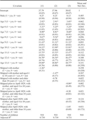
In Table 4, we report regression results that compare the heights of children that we identify as affiliated with a mother versus those that are not affiliated, controlling for age and sex. The first regression indicates that the children that we identify as (likely to have been) shipped with their mothers are 1.26 inches shorter than children of the same sex and age who are unaffiliated. The second regression in Table 4 interacts the “shipped with mother” effect on height with age indicators for children in two age groups: (1) children aged four to ten years, and (2) children aged more than 10 years. We find that for children aged ten years or less, the estimated height shortfall of affiliated children is roughly 1.47 inches. The estimated height shortfall for older affiliated children is 0.78 inches, although imprecisely estimated. Therefore, the results are consistent with the selectivity-bias hypothesis that children shipped to New Orleans for sale with their mothers were shorter and thus less valuable than children shipped without their mothers. The estimated effect is stronger for young children, although the difference between younger and older children is not robustly statistically significant. This finding lends support to the selectivity bias hypothesis for explaining the observed discounts associated with children in family groups, reported in Table 2.
As shown in Table 2, the magnitude of the family group discount associated with the sale of young children increased after 1829, when
HEIGHTS OF CHILDREN, AGED 4 TO 13 YEARS, SHIPPED BY NEW ORLEANS SLAVE TRADERS ORDINARY LEAST SQUARES REGRESSION RESULTS

* indicates the covariate is significantly different from zero at the 10 percent level.
Notes:
The dependent variable is the height of slaves in inches. The omitted variable represents a female slave, aged four years, shipped without her mother. Regression results for interactions of age and male indicator variables are not reported. Sample includes 120 manifests of slave traders identified from the New Orleans Conveyance Records. For the identification of children sold with mothers, see the text. Standard errors are listed in parentheses beneath regression coefficients.
Source:
Inward coastwise manifests, New Orleans, LA.
Louisiana law required all children under age 10 to be sold with their mothers. The third regression in Table 4 shows that the average heights of children traveling with their mothers after the passage of the 1829 law were lower, consistent with the increased price discount found in Table 2.
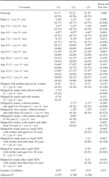
In Table 5, we report additional results including manifests for ships unrelated to the slave trade. These data serve two purposes. First, they provide a control group to test whether height differences measured in Table 4 between affiliated and unaffiliated children being sold can be properly attributed to the effects of selectivity bias in the sale of affiliated children sold with their mothers relative to stand-alone slave sales. If the same result were observed in manifest data unrelated to the slave trade, then that would suggest some other causal factor for this difference unrelated to selectivity bias in slave sales. Table 5 shows that the “shipped with mother effect,” per se, is zero. The covariate omitted from the regression equations refers to children shipped by non-traders and without an identified mother. As indicated by the regression coefficient for “Shipped with mother,” the heights of child slaves traveling on non-slave trader ships had similar heights irrespective of whether they were traveling with their mothers. In this larger sample, the indicator variables associated with slave trader vessels continue to show greater heights for children traveling without their mothers, especially for those under the age of 10 years.
A second purpose for analyzing height data from manifests is to compare the slave heights on slave traders' vessels with those traveling in the general population. Here the key finding is that slave children traveling on slave traders' ships, whether with their mothers or alone, were taller on average than slave children traveling on non-slave trader vessels. The magnitudes of the height differences for both child groups traveling on slave traders' vessels are large and statistically significant for slave children under the age of 10, although the magnitude of the effect is smaller and not statistically significant for children older than 10 who are traveling on a slave trader's ship with their mothers. We interpret this as evidence in favor of positive selectivity related to transportation cost, which caused the heights even of affiliated children en route for sale in New Orleans to be greater than the mean of the general population (as proxied by the average of children's heights from the non-slave trader manifests).
HEIGHTS OF CHILDREN, AGED 4 TO 13 YEARS, SHIPPED BY TRADERS AND NON-TRADERS, REGRESSION RESULTS

* indicates the covariate is significantly different from zero at the 5 percent level.
Notes:
The dependent variable is the height of slaves in inches. The omitted variable represents a female slave, aged four years, shipped without her mother by someone other than a slave trader. Regression results for interactions of age and male indicator variables are not reported. Sample includes 274 manifests, slave traders identified from the New Orleans Conveyance Records. For the identification of children sold with mothers, see the text. Standard errors are listed in parentheses beneath regression coefficients.
Source:
Inward coastwise manifests, New Orleans, LA.
Finally, we estimate the average heights of children traveling with their mothers (and shipped by slave traders) both before and after the passage of the 1829 law. Earlier, we found the increased legal protection of the mother-child relationship was associated with a decrease in the average height of children in such groups. In the third regression of Table 5, the affiliated children shipped by slave traders again were taller prior to the passage of this law. In contrast, the affiliated children shipped by traders after 1829 were on average only slightly taller (approximately .3 inches) than the children shipped by non-traders and the height difference was not statistically significant. The similarity in the heights of these affiliated children suggests that after the passage of this law, traders did not rigorously select these family groups and that only the children shipped separately were unusually tall for their age.
CONCLUSION
The existence of price discounts for slave families, when compared to stand-alone sales of slaves, has been known for some time.Footnote 23 Previous research attributes this price discount to a reduction in transaction costs associated with group sales. We find, however, no evidence of scale discounts for unrelated slaves. Families, rather than groups, account for the presence of price discounts.
Absent selectivity bias, slaves sold in family groups should have commanded higher prices. Fogel and Engerman argue that owners received economic value from maintaining families, which should have created a price premium rather than a price discount. Our primary explanation for the observed price discount for family groups, based on unobserved heterogeneity, suggests that the family members, if sold singly, would have commanded lower market prices than the unrelated slaves who were not sold in family groups. If the members of intact families had less valuable unobserved characteristics (such as shorter stature or poor health), this could explain why the group price is lower on average than the sum of the predicted prices for the individual family members when sold singly.
In order to test for the presence of unobserved heterogeneity, we searched for additional evidence that slaves sold in family groups were adversely selected. The coastwise manifests list the heights of slaves intended for sale in New Orleans. By comparing the heights of slaves (we infer were) shipped in family groups with those of slaves shipped separately, we demonstrate that children shipped with their mothers had shorter stature on average than children shipped singly. Because height is correlated with market value, the shorter stature of family slaves may account for the observed price discount observed for families.
The empirical literature on slave family discounts began with Fogel and Engerman's hypothesis that slave family sales should entail a premium, owing to the value of maintaining family ties, which they argued would be reflected in the values of slaves to their masters.Footnote 24 While our article does find some limited support for the existence of a nuclear family premium, ironically, we think our evidence of more general family discounts may provide stronger evidence of a positive price effect from preserving family ties. In our view, family discounts reflect the fact that the market attaches value to keeping some families together, especially in circumstances where one family member is weak or needy. That market decision itself depended on preexisting slave family preferences for family ties, which were only selectively permitted by the market.