



1 Introduction
Several industrial applications such as
 $\text{CO}_{2}$
sequestration, waste water disposal, engineered geothermal systems and reservoir stimulation involve the injection of a high pressure fluid in a porous medium. In all such applications, the rock permeability may be altered due to the growth of an induced tensile fracture, the activation of sealed weak planes, known as pre-existing fractures, or a combination of both effects (Ellsworth Reference Ellsworth2013; Gor, Stone & Prevost Reference Gor, Stone and Prevost2013). Understanding the interplay between fluid flow and changes in the rock permeability is essential for process optimization and modelling fluid and heat transport in hydraulically stimulated rocks.
In conventional reservoirs such as tight sandstones, the permeability enhancement is mainly due to the growth of a tensile fracture, whose geometry can be simple, and the contribution of activating pre-existing fractures can be neglected. Tensile fractures grow when the fluid pressure overcomes the compressive stresses acting on the fracture’s surfaces. Based on this mechanism, the interaction between the rock and fluid transport has been extensively studied both theoretically and experimentally (Cleary Reference Cleary1988; Savitski & Detournay Reference Savitski and Detournay2002; Lolon, Shaoul & Mayerhofer Reference Lolon, Shaoul and Mayerhofer2007; Lai et al. Reference Lai, Zhong, Dressaire, Wexler and Stone2015, Reference Lai, Zheng, Wexler and Stone2016). One of the first developed models assumes that the geometry of the fracture, i.e. its height and width, is known and independent of the fluid pressure (Howard & Fast Reference Howard and Fast1957). Other models relax the assumption of fixed aperture and relate the aperture to the fluid pressure through the rock’s elasticity (Perkins & Kern Reference Perkins and Kern1961; Geertsma & de Klerk Reference Geertsma and de Klerk1969; Nordgren Reference Nordgren1972). All such models are based on the premise that the volume of the fracture is equal to the amount of the injected fluid reduced by the total fluid lost from the fracture to the porous matrix through a process called leak off. The variations in modelling the growth of the tensile fracture come in the assumed fracture geometry, growth criterion and the type of fluid flowing through the fracture. For a detailed review on this field of studies, the reader is referred to the reviews of Adachi et al. (Reference Adachi, Sieberits, Peirce and Desroches2007), Detournay (Reference Detournay2016).
In shale rocks for example, where natural fractures are abundant, microseismic mappings, core analysis, backflow testing and well logging have shown that the injection of a high pressure fluid induces the formation of a complex fracture geometry (Warpinski & Teufel Reference Warpinski and Teufel1987; Sminchak et al. Reference Sminchak, Gupta, Byrer and Bergman2002; Warpinski et al. Reference Warpinski, Kramm, Heinze and Waltman2005; Majer et al. Reference Majer, Baria, Stark, Oates, Bommer, Smith and Asanuma2007). Upon injecting the fluid and initiating a tensile fracture, the tensile fracture interacts with pre-existing fractures. When the tensile fracture intersects a network of natural fractures, it gets arrested and fluid flow becomes controlled by the activation of natural fractures. The formation of a cluster of activated fractures has been shown to enhance gas production rate from stimulated rocks (Warpinski et al. Reference Warpinski, Kramm, Heinze and Waltman2005). Due to the complexity of the network geometry, modelling the coupling between fluid transport and mechanical response of the weak planes has been limited to the direct simulation of the activation process of a representative discrete network of fractures (Elmo & Stead Reference Elmo and Stead2010; Fu, Johnson & Carrigan Reference Fu, Johnson and Carrigan2012).
Simulation of discrete fracture networks (DFN), albeit detailed and flexible, requires extensive statistical analysis of a specific rock and the simulated number density of weak planes is limited by the computational power. Continuum modelling, on the other hand, is economical in the sense that it can be simple and can be applied to large networks that are not accessible using DFN. What limits the use of this approach is the difficulty in capturing the essential physics that control the growth behaviour of a cluster of activated natural fractures. This study attempts to develop a simple model that couples the pressure-driven flow of an incompressible fluid with the activation process of pre-existing weak planes.
The model is based on the following main assumptions: (i) natural fractures activate via a slippage mechanism following the Coulomb–Mohr criterion; (ii) stress perturbations due to the activation of neighbouring natural fractures are neglected; (iii) fluid flow is mainly within the activated natural fractures and the growth of a tensile fracture is neglected; and (iv) the rock is saturated with a fluid whose viscosity is much smaller than the viscosity of the injected fluid. In the slippage model, the activation of the pre-existing fractures occurs when the shear stress acting tangentially on the fracture’s surface is larger than the frictional force acting normally on the fracture’s surfaces. The frictional force is proportional to the overburden stress reduced by the fluid pressure saturating the fracture (Wang & Mao Reference Wang and Mao1979; Grasselli & Egger Reference Grasselli and Egger2002; Rutldege & Phillips Reference Rutldege and Phillips2003). Therefore, a natural fracture can be activated by either perturbing the stress field around the fracture or by increasing the fluid pressure saturating the natural fracture.
Perturbations in the stress can be due to the growth of tensile fractures or due to the activation of neighbouring natural fractures. Nagel et al. (Reference Nagel, Sanchez-Nagel, Zhang, Garcia and Lee2013) have shown that stress perturbations only activate a small number of fractures ahead of the tensile fracture tip. A larger number of fractures with no spatial preference are activated by perturbations to the pressure of the reservoir fluid. Networks generated via this mechanism are not necessarily connected. Both numerical simulations and simple analytical arguments have shown that the stress disturbance caused by a tensile fracture quickly decays away from its tip (Warpinski & Teufel Reference Warpinski and Teufel1987; Nagel et al. Reference Nagel, Sanchez-Nagel, Zhang, Garcia and Lee2013). Also, it has been shown experimentally and theoretically that a growing tensile fracture is most likely to be arrested as it intersects a natural fracture (Warpinski & Teufel Reference Warpinski and Teufel1987; Zhang, Jeffrey & Thiercelin Reference Zhang, Jeffrey and Thiercelin2007). Therefore, one can neglect the growth of a tensile fracture when modelling the activation of pre-existing fractures.
To describe the effects of reservoir fluid pressure perturbations on the activation of natural fractures, Shapiro & Dinske (Reference Shapiro and Dinske2009) have developed a simple equation for fluid pressure of a linearly compressible fluid in a cluster of natural fractures saturated with the same fluid. In their model, the interaction between the rock and the injected fluid is empirically modelled by assuming that the permeability of the cluster is a power law of pressure. Although this mechanism is only applicable for formations saturated with liquid, this model has been used widely to characterize fractured gas saturated rocks (Gischig & Wiemer Reference Gischig and Wiemer2013; Hummel & Shapiro Reference Hummel and Shapiro2013) due to its ability to interpret microseismic activities generated during the fracturing process. Similar to the case when stress perturbations activate the fractures, the created network via this mechanism is not inherently connected.
The activation of the fractures in the present model is based on pressure perturbations due to the change in fluid pressure as the injected fluid reaches the fractures. This applies when the viscosity of the injected fluid is much larger than that of the fluid saturating the natural fractures. The resulting mathematical equation describing the fluid pressure inside a growing cluster of activated fractures is similar to that describing viscous gravity currents where the evolution of the fluid pressure is described by a nonlinear diffusion equation which admits similarity solutions (Huppert & Woods Reference Huppert and Woods1995). The solution of this type of problems has been studied extensively (Acton, Huppert & Worster Reference Acton, Huppert and Worster2001; Pritchard, Woods & Hogg Reference Pritchard, Woods and Hogg2001; Huppert Reference Huppert2006; Pritchard Reference Pritchard2007; Pegler, Huppert & Neufeld Reference Pegler, Huppert and Neufeld2014; Hewitt, Neufeld & Balmforth Reference Hewitt, Neufeld and Balmforth2015; Zheng et al.
Reference Zheng, Guo, Christov, Celia and Stone2015) and been used to analyse several applications such as
 $\text{CO}_{2}$
sequestration and the disposal of waste water (Huppert & Neufeld Reference Huppert and Neufeld2006; Neufeld & Huppert Reference Neufeld and Huppert2009).
The paper is organized as follows. First, we will argue, in § 2, that percolation theory provides useful scalings to relate the properties of a network of activated fractures with the local fluid pressure. Such relations will allow us to derive a simple transport equation to couple fluid flow with the growth of a network of activated fractures. Thereafter, the growth of a single fracture system, which can be interpreted as a growing one-dimensional network of activated fractures, will be analysed in § 3. In this section, we obtain an analytical solution for the length of the fracture and show the conditions under which the competition of leakage and pressure-driven flow gives rise to a self-similar growth behaviour. After that, we analyse the growth of a two-dimensional cluster in § 4. Finally, the effects of operating conditions, fluid and rock properties on the cluster growth along with the expected microseismicity are discussed in § 5.
2 Theory
In this section, a model that couples the activation of a
 $D$
-dimensional network of natural fractures and fluid transport within the activated fractures will be developed. In particular, we will consider the case where percolation theory can be used to couple the fluid pressure with the local hydraulic conductivity of the network of activated fractures. To elucidate this idea, the discussion is presented as follows. First, percolation theory is briefly explained and the connection between the theory and the growth of a network of activated fractures when the fluid pressure is constant and uniform will be discussed. Then, the different growth behaviours of the cluster that occur when the injection rate is maintained at different values or ramped up at different rates will be discussed and we will identify the regime where the proposed coupling model applies. Finally, a general transport equation of the injected fluid will be introduced.
2.1 Percolation theory and fracture activation under constant fluid pressure
In percolation theory, one starts with connected closed bonds and opens them with a certain probability. Percolation theory states that one infinite percolating cluster is formed when a threshold fraction,
 $F_{c}$
, of the bonds is opened (Stauffer Reference Stauffer1979). The value of
 $F_{c}$
depends on the topology of the formed network. For instance,
 $F_{c}=1/2$
for a two-dimensional square lattice of bonds and
 $F_{c}=1$
for a one-dimensional network. Moreover, several bulk properties of the percolating network scale with the difference between the fraction of opened bonds,
 $F$
, and
 $F_{c}$
when
 $F-F_{c}\ll F_{c}$
. That is
 $X\sim |F-F_{c}|^{a}$
where
 $X$
is a bulk property of interest and
 $a$
is a universal scaling exponent that only depends on the dimension of the network and not on its topological details.
Among several bulk properties that follow universal scalings are the percolating network’s correlation length, its porosity and its hydraulic conductivity. The correlation length of a network,
 $\unicode[STIX]{x1D709}$
, is defined as the average distance between two points in the network and it is a measure of how sparse the network is. Above the percolation threshold, the percolating cluster’s correlation length is the average radius of gyration of the clusters of closed bonds. Portions of the percolating network smaller than the correlation length look fractal, while the network looks homogeneous when the length scale is larger than the correlation length. As the fraction of opened bonds increases beyond
 $F_{c}$
, the correlation length decays as
 $\unicode[STIX]{x1D709}\sim \unicode[STIX]{x1D709}_{0}(F-F_{c})^{-\unicode[STIX]{x1D708}}$
where
 $\unicode[STIX]{x1D709}_{0}$
is the correlation length of the existing bonds in the system. For example, if the bonds form a square lattice,
 $\unicode[STIX]{x1D709}_{0}$
is equal to the lattice spacing. In two dimensions,
 $\unicode[STIX]{x1D708}=4/3$
while it is estimated to be about
 $0.88$
in three dimensions (Sahimi Reference Sahimi2011).
Similarly, the fraction of the bonds that are open and belong to the percolating cluster,
 $S$
, and the percolating network’s hydraulic conductivity,
 $K$
, scale as
 $S\sim \unicode[STIX]{x1D709}^{-\unicode[STIX]{x1D6FD}/\unicode[STIX]{x1D708}}$
and
 $K\sim k_{0}\unicode[STIX]{x1D709}^{-\unicode[STIX]{x1D716}/\unicode[STIX]{x1D708}}$
, respectively.
 $k_{0}$
is the permeability of the network when all the bonds are opened. For
 $D=2$
,
 $\unicode[STIX]{x1D6FD}=5/36$
and
 $\unicode[STIX]{x1D716}\approx 1.3$
, while, for
 $D=3$
,
 $\unicode[STIX]{x1D6FD}\approx 0.42$
and
 $\unicode[STIX]{x1D716}\approx 2.0$
(Stauffer & Aharony Reference Stauffer and Aharony1994; Kozlov & Lagues Reference Kozlov and Lagues2010; Wang et al.
Reference Wang, Zhou, Zhang, Garoni and Deng2013). These scalings are valid when
 $\unicode[STIX]{x1D709}_{0}\ll \unicode[STIX]{x1D709}\leqslant B$
where
 $B$
is the system size. If
 $\unicode[STIX]{x1D709}\gg B\gg \unicode[STIX]{x1D709}_{0}$
, the bulk properties scale with
 $B$
, e.g.
 $S\sim B^{-\unicode[STIX]{x1D6FD}/\unicode[STIX]{x1D708}}$
. For more details about percolation theory and its application to fluid transport, the reader is referred to Stauffer & Aharony (Reference Stauffer and Aharony1994), Sahimi (Reference Sahimi2011) and Hunt, Ewing & Ghanbarian (Reference Hunt, Ewing and Ghanbarian2014).
Returning to the fracturing process, following the slippage mechanism, a weak plane will undergo slippage when the stress tangent to the plane is larger than the product of a friction coefficient and an effective normal stress. If the stress field is constant, each discontinuity is associated with a critical fluid pressure,
 $P_{c}$
, the fluid has to reach in order for slippage to occur:
 $$\begin{eqnarray}P_{c}=\unicode[STIX]{x1D70E}_{n}-\frac{\unicode[STIX]{x1D70E}_{t}}{f_{r}},\end{eqnarray}$$
where
 $\unicode[STIX]{x1D70E}_{t}$
,
 $\unicode[STIX]{x1D70E}_{n}$
are the tangential and normal stresses acting on the fracture, respectively, and
 $f_{r}$
is the friction coefficient. The initial aperture of the pre-existing discontinuity is very small such that fluid flow is negligible. Upon slippage, its aperture becomes large enough to allow fluid flow. The creation of fluid filling volume is due to the mismatch between the asperities of the two surfaces induced by slippage. To simplify the model, the effects of stress perturbation due to surface displacement are ignored. Hence, the time variation in the aperture within the growing fracture is ignored and a characteristic hydraulic aperture is assumed. When the viscosity of the fluid saturating the weak planes is much smaller than that of the injected fluid, the fracturing fluid’s pressure controls the activation process as the fluid perturbs the pressure within the natural fracture.
If the viscous pressure drop is negligible and the fluid is injected at a constant pressure, the fraction of pre-existing weak planes whose critical pressure is below the fluid’s pressure can open. When the fractures’ critical pressures follow a homogeneous distribution, the fraction of fractures that have a critical pressure below the fluid pressure, denoted as
 $F$
, is given by:
 $$\begin{eqnarray}F(P)=\int _{P_{c_{min}}}^{P}f_{pc}(x)\,\text{d}x,\end{eqnarray}$$
where
 $P$
is the fluid pressure and
 $f_{pc}(x)$
is the probability distribution function of the fractures’ critical pressures.
 $f_{pc}$
becomes random when the critical pressures are uncorrelated with the fracture’s orientation. This can be the case when the stress field is heterogeneous over large length scales.
 $P_{c_{min}}$
is the minimum critical pressure in the distribution. As the injected fluid propagates through the network of activated fractures, some of the fractures that have critical pressures below the fluid pressure will remain unactivated. These fractures are connected to the activated fracture network via weak planes with critical pressures that are larger than the fluid pressure. Therefore, they will not be activated and the injected fluid will be constrained within the formed percolating network.
The conformity of the percolation problem and the mechanism of activating pre-existing weak planes under a constant pressure can be stated as follows. The fraction of opened bonds in percolation theory,
 $F$
, corresponds to the fraction of natural fractures whose critical pressure is lower than
 $P$
. The fraction of the opened bonds that belong to the percolating network,
 $S$
, represents the fraction of activated fractures. The threshold fluid pressure,
 $P_{cc}$
, needed to form a percolating network of activated fractures can be obtained by taking the inverse of (2.2) evaluated at
 $F=F_{c}$
. Since the value of
 $F_{c}$
depends on the topology of the network and its dimension, one expects the same dependence for the value of
 $P_{cc}$
. Additionally, the value of
 $P_{cc}$
depends on the functional form of
 $f_{pc}$
.
To relate the bulk properties of the activated network of fractures to the fluid pressure, equation (2.2) can be linearized so that:
 $$\begin{eqnarray}F-F_{c}=k_{f}(P-P_{cc}),\end{eqnarray}$$
where
 $k_{f}$
is a proportionality constant whose order of magnitude is equal to the reciprocal of the probability distribution’s standard deviation,
 $\unicode[STIX]{x1D6FF}_{pc}$
. For a normal distribution, for instance,
 $k_{f}=1/(\sqrt{2\unicode[STIX]{x03C0}}\unicode[STIX]{x1D6FF}_{pc})$
. This linearization applies when
 $F-F_{c}\ll F_{c}$
; the regime where the universal scalings apply. Given (2.3), the dependence of the network properties on the fluid pressure can be written as:
 $$\begin{eqnarray}\displaystyle & \displaystyle \unicode[STIX]{x1D709}=\unicode[STIX]{x1D709}_{0}k_{\unicode[STIX]{x1D709}}[k_{f}(P-P_{cc})]^{-\unicode[STIX]{x1D708}}, & \displaystyle\end{eqnarray}$$
 $$\begin{eqnarray}\displaystyle & \displaystyle S=k_{s}[k_{f}(P-P_{cc})]^{\unicode[STIX]{x1D6FD}}, & \displaystyle\end{eqnarray}$$
 $$\begin{eqnarray}\displaystyle & \displaystyle K=k_{0}k_{k}[k_{f}(P-P_{cc})]^{\unicode[STIX]{x1D716}}, & \displaystyle\end{eqnarray}$$
where
 $k_{\unicode[STIX]{x1D709}}$
,
 $k_{s}$
and
 $k_{k}$
are dimensionless proportionality constants and depend on the geometry of the network and its dimension while the critical exponents are universal and only depend on the dimension of the network.
 $\unicode[STIX]{x1D709}_{0}$
is the correlation length of the existing natural fractures and its equivalent length scale in regular percolation is the lattice spacing.
2.2 Network formation under controlled injection rate
Previously, it has been shown that when the fluid pressure is constant, the dependence of the activation of natural fractures on the fluid pressure leads to the formation of a network whose bulk properties follow the same universality scalings found in regular percolation. Now, we consider the case where the injection rate is controlled and show that one can use the derived scalings, equations (2.4)–(2.6), locally to model fluid transport within the fractured rock.
There are four length scales that control the activation process: (i) the average length of the pre-existing weak planes,
 $L_{av}$
; (ii) the correlation length of pre-existing natural fractures,
 $\unicode[STIX]{x1D709}_{0}$
, that is related to the second moment of the fractures’ length distribution (Balberg et al.
Reference Balberg, Anderson, Alexander and Wagner1984); (iii) a characteristic correlation length of the cluster of activated natural fractures
 $\unicode[STIX]{x1D709}_{ch}$
; and (iv) the cluster’s radius,
 $R$
.
 $\unicode[STIX]{x1D709}_{0}$
is the average distance between these fractures and is of the order of the fracture spacing. If the density of these fractures is large and their lengths are of the same order of magnitude, the average spacing and hence
 $\unicode[STIX]{x1D709}_{0}$
become of the same order as
 $L_{av}$
. In this case, the network of pre-existing natural fractures is homogeneous, that is its fractal dimension is equal to the Euclidean dimension of the network. However, if the density approaches a threshold value,
 $\unicode[STIX]{x1D709}_{0}\rightarrow \infty$
producing a fractal network of pre-existing natural fractures. In this paper, we are limiting ourselves to the case in which
 $\unicode[STIX]{x1D709}_{0}$
is finite and very close to
 $L_{av}$
.
 $\unicode[STIX]{x1D709}_{ch}$
is defined as the average radius of gyration of the clusters of unactivated fractures within the network of activated fractures. It is a function of the ratio of the pressure drop across the network of activated fractures to
 $\unicode[STIX]{x1D6FF}_{pc}$
, i.e.
 $\unicode[STIX]{x1D709}_{ch}\sim (P_{ch}/\unicode[STIX]{x1D6FF}_{pc})^{-\unicode[STIX]{x1D708}}$
.
 $P_{ch}$
is the characteristic pressure drop across the cluster of activated fractures which will be derived later on. If the viscous pressure drop is negligible,
 $\unicode[STIX]{x1D709}_{ch}\rightarrow \infty$
and when an extremely viscous fluid is injected at a high rate,
 $\unicode[STIX]{x1D709}_{ch}$
is expected to approach
 $\unicode[STIX]{x1D709}_{0}$
.
Type of networks produced based on the importance of the viscous pressure drop. In all cases, the pre-existing natural fractures form a homogeneous network, i.e.
 $\unicode[STIX]{x1D709}_{0}\sim O(L_{av})$
. (a) Shows a fractal network produced when the viscous pressure drop is not important and the fracturing process is controlled by the distribution of the critical pressures. (b) Shows a homogeneous network produced when the viscous pressure drop overcomes the variability of the critical pressures. (c) Shows a network that looks the same as a network near the percolation threshold at the length scale
 $\unicode[STIX]{x1D709}_{ch}$
. Over the length scale of the radius, the network looks heterogeneous.

Depending on the competition between the viscous pressure drop required to drive the flow and the pressure change induced by activating a pre-existing fracture, the growth dynamics can behave differently. When the viscous pressure drop is negligible when compared to the variability of the critical pressures, a scale-invariant fractal network is produced while a homogeneous network at all length scales is produced when the viscous pressure drop is dominant in the fracturing process. Between these two extreme cases, an intermediate regime can be identified where the viscous pressure drop is important over the cluster radius but can be neglected over the length scale,
 $\unicode[STIX]{x1D709}_{ch}$
. In this case, the produced network has a structure at small length scales similar to a percolating network formed near the percolation threshold and looks heterogeneous over the cluster radius. In all three cases, the injected fluid pressure must be at least equal to the threshold critical pressure,
 $P_{cc}$
.
In the first extreme case where the viscous pressure drop is negligible, i.e.
 $\unicode[STIX]{x1D709}_{0}\sim O(L_{av})\ll R\ll \unicode[STIX]{x1D709}_{ch}$
, the network of activated fractures is fractal. Its structure is the same as a percolating network formed at the threshold value as shown in figure 1(a). In this case, the injected fluid activates the accessible fractures with the smallest critical pressure and its growth behaviour can be described by the invasion percolation without trapping algorithm (Wilkinson & Willemsen Reference Wilkinson and Willemsen1983). In this algorithm, each bond in a network is associated with a random resistance to opening. At each simulation step, a bond with the lowest resistance that is connected to the network of opened bonds is opened. Bonds with a low resistance connected to the network via a path of bonds with higher resistances remain closed. This algorithm produces a fractal network with the same fractal dimension,
 $1.9$
when
 $D=2$
, as a network generated at the percolation threshold following regular percolation rules.
A recent study by Tayeb et al. (Reference Tayeb, Sahimi, Aminzadeh and Sammis2013) has argued that a hydraulically fractured network of natural fractures, in the Geysers geothermal field in northeast California, has the same fractal dimension as a percolation cluster formed at the threshold value. The results were interpreted by a model developed by Sahimi, Robertson & Sammis (Reference Sahimi, Robertson and Sammis1993) where large scale heterogeneities in the resistances to activate a fracture lead to a random fracturing process similar to the process used to form a percolating network. As mentioned in § 2.2, heterogeneity in the stress field, at length scales larger than
 $L_{av}$
, can lead to a random distribution of critical pressures. In order for the randomness in the resistances to control the cluster growth and produce a fractal network, our model predicts that the variability of the critical pressures must be much larger than the viscous pressure drop required to drive the flow, i.e.
 $\unicode[STIX]{x1D709}_{0}\approx L_{av}\ll R\ll \unicode[STIX]{x1D709}_{ch}$
.
The other extreme case to consider is when the viscous pressure drop within the fractures is dominant. If
 $\unicode[STIX]{x1D709}_{ch}\sim \unicode[STIX]{x1D709}_{0}\ll R$
, one expects that the injected fluid will easily overcome the largest resistance and hence will activate all natural fractures at the fluid front. The growth behaviour in this case can be described by a linear diffusion equation and the network produced via this behaviour looks homogeneous at all length scales as shown in figure 1(b). The fractal dimension of the produced network is the same as the Euclidean dimension of space embedding the network. This case is not relevant to fractured geological reservoirs as Sahimi (Reference Sahimi2011) has shown that all networks of activated fractures either form a scale-invariant fractal network or a network that is fractal at small length scales and homogeneous at large length scales.
Between such extreme cases, one can identify a regime where the viscous pressure drop across the cluster of activated fractures is important but it can be neglected over distances of order
 $\unicode[STIX]{x1D709}_{ch}$
, where
 $$\begin{eqnarray}\unicode[STIX]{x1D709}_{0}\ll \unicode[STIX]{x1D709}_{ch}\ll R.\end{eqnarray}$$
The produced network in this regime is expected to be near the percolation threshold throughout the cluster. Below
 $\unicode[STIX]{x1D709}_{ch}$
, it looks fractal while the network’s properties are heterogeneous at large length scales as shown in figure 1(c). In this paper, a model is developed to describe the growth of a network of activated fractures when (2.7) applies. If the viscous pressure drop is negligible over
 $\unicode[STIX]{x1D709}_{ch}$
and
 $\unicode[STIX]{x1D709}_{ch}\ll R$
, a local fluid pressure can be defined over that region. In § 2.1, it has been shown that when the many connected fractures feel a constant fluid pressure, their activation will lead to the formation of a percolating network. Furthermore, the properties of the activated network will scale with the fluid pressure in that region. Therefore, one can see that the local properties of the network can be described using (2.4)–(2.6) if the local correlation length is much larger than
 $\unicode[STIX]{x1D709}_{0}$
but is much smaller than the cluster radius. Since the viscous pressure drop required to drive the flow of the fluid is important over the cluster radius, the local properties of the network such as the fraction of activated fractures,
 $S$
, and the permeability of the network,
 $K$
, will evolve spatially and temporally as fluid is injected. Hence, one can couple fluid transport with the activation of natural fractures through the dependence of
 $S$
and
 $K$
on the fluid pressure. Since the fluid pressure has to be at least equal to
 $P_{cc}$
to form a percolating network, it is expected that the pressure at the edge of the cluster will be very close to
 $P_{cc}$
and the network will look fractal in that region.
A sketch of the cluster of activated fractures. The solid lines represent the network of activated fractures while the dashed bonds represent the weak planes with critical pressures below the local pressure that nonetheless remain unactivated. On the right-hand side, the fluid pressure is slightly larger than the threshold critical pressure to ensure the formation of a percolating network. As the fluid pressure increases, the density of the percolating network increases. The network on the left represents a denser percolating network than the one on the right because the local pressure is higher due to the viscous pressure drop required to drive the flow.

Figure 2 is an illustration of how the activated fracture network will look when (2.7) applies. The middle cartoon in the figure shows the entire cluster of activated fractures if the pre-existing natural fractures form a square lattice. The right-hand sketch shows how a network of activated fractures is expected to form when the local pressure is slightly larger than the threshold critical pressure,
 $P_{cc}$
. The solid lines represent the activated fracture network and the dashed lines are disconnected fractures which remain unactivated despite having critical pressures below the local fluid pressure. Since the pressure drop required to drive the flow is important over the cluster’s radius, the pressure in the interior region of the network is higher than
 $P_{cc}$
and, hence, the network there is more connected as shown in the left hand sketch. Based on this picture of how a network of activated fractures propagates, we shall introduce a continuum model that couples fluid flow with permeability and porosity evolution within a porous media.
2.3 Transport equation
The fractured rock is modelled as a dual porosity medium: a primary porosity due to interconnected activated fractures and a secondary porosity due to the pores of the rock matrix. Fluid flow in the secondary porosity is coupled with a pressure-driven flow within the primary porosity through a process called leak off. Each natural fracture within the primary porosity is assumed to be activated when the fluid pressure reaches a critical value. The activation process of a network of fractures with random resistances can be described by percolation theory. Hence, fluid flow within the primary porosity is controlled by the interconnectivity of the activated fractures but not by the detailed geometry of the formed network. Equation (2.7) applies and thus the primary porosity is allowed to change with time and position as weak planes are fractured. The secondary porosity is assumed to be constant and unaffected by the pressure of the leaked fluid. The time scale at which the primary porosity evolves is much larger than the time scale to completely activate a pre-existing weak plane.
To relate fluid flow with the growth of a cluster of fractures, a local mass balance that accounts for changes in the primary porosity upon the injection of the fracturing fluid can be used:
 $$\begin{eqnarray}\unicode[STIX]{x1D700}\frac{\unicode[STIX]{x2202}S}{\unicode[STIX]{x2202}t}+\unicode[STIX]{x1D735}\boldsymbol{\cdot }\boldsymbol{q}+V_{l}=0,\end{eqnarray}$$
where
 $\unicode[STIX]{x1D700}$
is the primary porosity if all the local pre-existing fractures are activated, which is assumed to be constant when considering a homogeneous number density of the natural weak planes.
 $V_{l}$
accounts for the total leakage rate from the local network per unit medium volume.
 $\boldsymbol{q}$
is the superficial flux of the fluid through the network and it can be described using Darcy’s law where the permeability is given by (2.6).
 $\unicode[STIX]{x1D700}S$
is the primary porosity and its dependence on the fluid pressure is given by (2.5).
Two boundary conditions can be used to fully define the problem. One can specify the flux at the injection point and the fluid pressure at the edge of the cluster. Since a percolating network forms when the fluid pressure is at least equal to
 $P_{cc}$
, the fluid pressure at the edge of the cluster can be set to be equal to
 $P_{cc}$
. To find how the cluster radius grows with time, one can perform a volume integral on (2.8) and apply the flux at the injection point and zero flux past the moving front of the cluster,
 $R(t)$
, to get:
 $$\begin{eqnarray}\unicode[STIX]{x1D700}\frac{\unicode[STIX]{x2202}}{\unicode[STIX]{x2202}t}\left(\int S\,\text{d}V\right)=q_{inj}-\int V_{l}\,\text{d}V,\end{eqnarray}$$
where
 $q_{inj}$
is the flux at the injection point.
The above system of equations governs the growth behaviour of a
 $D$
-dimensional network of activated fractures by coupling fluid transport and changes in the rock’s porosity. As can be seen from (2.8), the competition between the leakage term and the pressure-driven flow controls how the primary porosity evolves. To demonstrate how this competition can lead to two distinct self-similar growth behaviours, we will first analyse the growth of a one-dimensional network. For this simple case, an analytical solution for the length of the network can be obtained. Furthermore, the analysis for this network will prove useful in justifying some of the assumptions that will be used to solve for the two-dimensional case. The solution for a two-dimensional network will be presented in § 4.
3 Single fracture growth
In this section, the effects of the viscous pressure drop and fluid loss on the activation of natural fractures are analysed by modelling the growth of a single fracture. Several studies have shown that the activation of natural fractures due to slippage forms a cloud of microseismic events. In some cases, the cloud can form a planar structure that propagates in a particular direction during the activation process (Philips Reference Philips2000; Tezuka & Niitsuma Reference Tezuka and Niitsuma2000; Asanuma et al. Reference Asanuma, Nozaki, Niitsuma and Wyborn2005). The formation of such clouds has been interpreted as either due to slippage of the asperities within a large planar fracture system or due to the activation of natural fractures that are anisotropically aligned in a preferred direction. Both interpretations yield the same mathematical formulation to describe the growth of the planar cloud. Since the latter is most commonly accepted and represents a one-dimensional case of the model presented in (2.8), we will adopt it in this section.
The single fracture represents a linear network of connected fractures and its growth results from the continuous activation of these fractures. The length of the fracture represents the position of the cloud’s edge. To make distinction between the network and the fractures, we are going refer to the fractures forming the network as discontinuities and the linear network as the single fracture. Using the model, several limiting cases are discussed. The case where the effects of the pressure drop within the fracture on leakage can be neglected is considered and an analytical solution for the fracture’s length is derived. Then, the effects of ignoring the variation in the leakage velocity within the fracture is discussed. Finally, we present the full numerical solution of the single fracture model.
Assuming that an infinite fracture is composed of connected natural discontinuities that form a linear path, the growth of the network can be viewed as growing a single fracture under the following conditions: (i) the activation conditions of the discontinuities are similar and (ii) the length scale of the network is much larger than the average length of these discontinuities. Since the continuous growth of the linear network requires the activation of its constituents, the pressure of the injected fluid must be larger than their critical pressure. Their average critical pressure,
 $P_{c}$
, is assumed to control the growth of the single fracture. This assumption is valid when the difference in the critical pressure of the discontinuities is much smaller than
 $P_{c}$
. Hence, the pressure at the fluid front is equal to
 $P_{c}$
.
3.1 Governing equations
Assuming that the one-dimensional network forms a rectangular fracture, equation (2.8) can be reduced to:
 $$\begin{eqnarray}\frac{\text{d}}{\text{d}x}q+2v_{l}=0.\end{eqnarray}$$
In this equation,
 $q$
is the fluid flux per width and the fluid flows in the
 $x$
direction whereas the leaking fluid flows perpendicular to the two fracture surfaces into the rock matrix. The leakage term in (2.8) becomes the local leakage velocity,
 $v_{l}$
, that is defined as the volumetric flow rate per surface area. The porosity term,
 $\unicode[STIX]{x2202}S/\unicode[STIX]{x2202}t$
, in (2.8) is set to be zero since the local porosity consists of the volume of the locally activated discontinuity. Therefore, it will not change with time when its aperture is assumed to be constant. This assumption holds when the pressure within the activated discontinuities does not overcome the far-field normal stress acting on asperities on the fracture surfaces that prop the fracture open and the effects of shear dilation following the initial activation of a discontinuity are ignored. Shear dilation results from stress perturbations due to slippage and is a function of the magnitude of displacement and the surface roughness (Willis-Richards, Watanabe & Takahashi Reference Willis-Richards, Watanabe and Takahashi1996; Olsson & Barton Reference Olsson and Barton2001). Since the network’s conductivity was described by an effective permeability when deriving (2.8), a hydraulic aperture,
 $b$
, will be used for the one-dimensional network. Since the competition between pressure-driven flow and leakage depends on a characteristic conductivity parameter, changes in the fracture’s aperture are not expected to change the qualitative growth behaviour of the fracture.
The pressure at the fluid front
 $L(t)$
must be equal to
 $P_{c}$
, in order for slippage to occur and maintain the continuous growth of the activated fracture. Hence, one can use the following boundary condition:
 $$\begin{eqnarray}P=P_{c},\quad \text{at }x=L(t).\end{eqnarray}$$
The other boundary condition required to solve (3.1) can be written as:
 $$\begin{eqnarray}q=\frac{Q}{w},\quad \text{at }x=0,\end{eqnarray}$$
through which the injection rate at the injection well
 $Q$
can be specified.
Finally, equation (2.9) to describe the growth of a rectangular fracture can be written as:
 $$\begin{eqnarray}wb\frac{\text{d}L}{\text{d}t}=Q-2w\int _{0}^{L}v_{l}\,\text{d}x,\end{eqnarray}$$
where
 $w$
is the fracture’s width and
 $b$
is the activated fracture’s aperture.
To completely define the problem, constitutive relations are needed to describe the flux within the fracture and the leakage velocity. Since the length of the activated fracture is of the order of metres while the aperture is of the order of micro- to millimetres, the flux within the fracture for a Newtonian fluid can be described by the cubic law (Zimmerman & Bodvarsson Reference Zimmerman and Bodvarsson1996):
 $$\begin{eqnarray}q=-\frac{b^{3}}{12\unicode[STIX]{x1D707}}\frac{\unicode[STIX]{x2202}P}{\unicode[STIX]{x2202}x},\end{eqnarray}$$
where
 $\unicode[STIX]{x1D707}$
is the fracturing fluid viscosity. The leaked fracturing fluid is assumed to displace the fluid saturating the rock, whose viscosity is much smaller than that of the injected fluid. The pressure at the interface between the two fluids is assumed to be equal to the pressure of the saturating fluid,
 $P_{f}$
. If capillary effects are important, i.e. when the surface tension per pore width is comparable with
 $P_{c}$
, one can account for it in the definition of
 $P_{f}$
. Given a pressure gradient imposed by the difference between the pressure of the fracturing fluid at the fracture surface and
 $P_{f}$
, the leaking fluid is assumed to propagate following Darcy’s law. This process is denoted as fluid seepage and can be described by (Howard & Fast Reference Howard and Fast1957):
 $$\begin{eqnarray}v_{l}=\unicode[STIX]{x1D700}_{m}\frac{\text{d}l_{w}}{\text{d}t}=\frac{k_{m}}{\unicode[STIX]{x1D707}}\frac{P-P_{f}}{l_{w}},\end{eqnarray}$$
where
 $l_{w}$
is the distance between the fracture surface and the interface, and
 $\unicode[STIX]{x1D700}_{m}$
and
 $k_{m}$
are the rock’s porosity and permeability, respectively. If the viscous pressure drop is much smaller than
 $(P_{c}-P_{f})$
, one can assume a quasi-steady fluid pressure at the surface of the fracture and, hence, the solution of (3.6) yields:
 $$\begin{eqnarray}v_{l}=C\sqrt{\frac{P-P_{f}}{t-t^{\prime }}},\end{eqnarray}$$
where
 $C=\sqrt{(k_{m}\unicode[STIX]{x1D700}_{m})/2\unicode[STIX]{x1D707}}$
. The fracturing fluid starts to leak from a point
 $x$
in space at
 $t^{\prime }$
; the time at which the fracture tip reaches that point. The range of validity of the quasi-steady assumption is discussed in appendix A.
By substituting (3.7) and (3.5) into (3.1) and (3.4), the system of equations governing the growth of the fracture becomes:
 $$\begin{eqnarray}\displaystyle & \displaystyle b\frac{\text{d}L}{\text{d}t}=Q/w-2C\int _{0}^{L}\sqrt{\frac{P-P_{f}}{t-t^{\prime }(x)}}\,\text{d}x, & \displaystyle\end{eqnarray}$$
 $$\begin{eqnarray}\displaystyle & \displaystyle \frac{\unicode[STIX]{x2202}^{2}P}{\unicode[STIX]{x2202}x^{2}}=\frac{24\unicode[STIX]{x1D707}C}{b^{3}}\sqrt{\frac{P-P_{f}}{t-t^{\prime }(x)}}, & \displaystyle\end{eqnarray}$$
 $$\begin{eqnarray}\displaystyle & \displaystyle P=P_{c},\quad \text{at }x=L(t), & \displaystyle\end{eqnarray}$$
 $$\begin{eqnarray}\displaystyle & \displaystyle \frac{\unicode[STIX]{x2202}P}{\unicode[STIX]{x2202}x}=\frac{-12\unicode[STIX]{x1D707}Q}{wb^{3}},\quad \text{at }x=0, & \displaystyle\end{eqnarray}$$
with the initial condition
 $L(0)=0$
.
The following characteristic parameters will be used to non-dimensionalize the above system of equation:
 $$\begin{eqnarray}\displaystyle & \displaystyle t_{ch}=\frac{\unicode[STIX]{x1D707}b^{2}}{2k_{m}\unicode[STIX]{x1D700}_{m}(P_{c}-P_{f})}, & \displaystyle\end{eqnarray}$$
 $$\begin{eqnarray}\displaystyle & \displaystyle L_{ch}=\frac{Q\unicode[STIX]{x1D707}b}{2wk_{m}\unicode[STIX]{x1D700}_{m}(P_{c}-P_{f})}, & \displaystyle\end{eqnarray}$$
 $$\begin{eqnarray}\displaystyle & \displaystyle P_{ch}=\frac{6\unicode[STIX]{x1D707}^{2}Q^{2}}{w^{2}b^{2}k_{m}\unicode[STIX]{x1D700}_{m}(P_{c}-P_{f})}, & \displaystyle\end{eqnarray}$$
 $$\begin{eqnarray}\displaystyle & \displaystyle l_{w}^{ch}=\frac{b}{\unicode[STIX]{x1D700}_{m}}, & \displaystyle\end{eqnarray}$$
where
 $t_{ch}$
is the time at which the activated fracture extends for a large enough length,
 $L_{ch}$
, for the leakage rate to significantly slow down the growth rate. For typical rocks with permeabilities ranging from
 $10^{-19}$
to
 $10^{-16}~\text{m}^{2}$
and
 $P_{c}-P_{f}$
of the order of MPa, the characteristic time ranges from a few seconds for water injected in a high permeability rock to years for a viscous fluid such as a cross-linked gel whose viscosity can range from 100 to 1000 cP injected in an ultra-low permeable rock (Montgomery Reference Montgomery and Jeffery2013). The characteristic pressure,
 $P_{ch}$
, is the viscous pressure drop required to drive the flow of the fracturing fluid over
 $L_{ch}$
.
 $l_{w}^{ch}$
is the characteristic penetration length into the rock matrix. In order to avoid interference between fractures,
 $l_{w}^{ch}$
must be much smaller than the average spacing between two fractures. Since the aperture of typical fractures is of the order of a few millimetres, the penetration length will be of the order of a few centimetres which is much smaller than a typical
 $O$
(10) m fracture spacing.
Now, let
 $\bar{t}=t/t_{ch}$
,
 $\bar{P}=(P-P_{c})/P_{ch}$
,
 $\bar{L}=L/L_{ch}$
and substitute these dimensionless variables into (3.8) through (3.11) to get:
 $$\begin{eqnarray}\displaystyle & \displaystyle \frac{\text{d}\bar{L}}{\text{d}\bar{t}}=1-\int _{0}^{\bar{L}}\sqrt{\frac{\unicode[STIX]{x1D6E5}_{pc}\bar{P}+1}{\bar{t}-\bar{t^{\prime }}}}\,\text{d}\bar{x}, & \displaystyle\end{eqnarray}$$
 $$\begin{eqnarray}\displaystyle & \displaystyle \frac{\unicode[STIX]{x2202}^{2}\bar{P}}{\unicode[STIX]{x2202}\bar{x^{2}}}=\sqrt{\frac{\unicode[STIX]{x1D6E5}_{pc}\bar{P}+1}{\bar{t}-\bar{t^{\prime }}}}, & \displaystyle\end{eqnarray}$$
 $$\begin{eqnarray}\displaystyle & \displaystyle \bar{P}=0,\quad \text{at }x=\bar{L}(\bar{t}), & \displaystyle\end{eqnarray}$$
 $$\begin{eqnarray}\displaystyle & \displaystyle \frac{\unicode[STIX]{x2202}\bar{P}}{\unicode[STIX]{x2202}\bar{x}}=-1,\quad \text{at }x=0, & \displaystyle\end{eqnarray}$$
with the initial condition of zero length at
 $t=0$
.
 $\unicode[STIX]{x1D6E5}_{pc}\equiv P_{ch}/(P_{c}-P_{f})$
measures the importance of pressure variation within the fracture on the leakage rate. For instance, the leakage rate becomes independent of the viscous pressure drop along the fracture when
 $\unicode[STIX]{x1D6E5}_{pc}\rightarrow 0$
.
Before introducing the numerical solution of the above system of equations for different values of
 $\unicode[STIX]{x1D6E5}_{pc}$
, several limiting cases will be discussed. We will show that when
 $\unicode[STIX]{x1D6E5}_{pc}=0$
, two similarity solutions for the fluid pressure can be obtained depending on the importance of the leakage rate in affecting the growth of the fracture. Thereafter, we show that the similarity exponents found in this case are retained even when one further simplifies the leakage rate by assuming that
 $t^{\prime }=0$
and
 $\unicode[STIX]{x1D6E5}_{pc}=0$
.
3.2 Similarity solutions when the pressure variation in the fracture is negligible
When
 $\unicode[STIX]{x1D6E5}_{pc}=0$
, the leakage velocity is not sensitive to fluid pressure variations in the fracture and therefore (3.16) and (3.17) decouple. In this case, one can obtain an analytical solution for the fracture length and identify two regimes where the growth behaves in a self-similar fashion. The complete solution of (3.16), when
 $\unicode[STIX]{x1D6E5}_{pc}=0$
, is given by:
 $$\begin{eqnarray}\bar{L}=\frac{1}{\unicode[STIX]{x03C0}}\left[\text{e}^{\unicode[STIX]{x03C0}\bar{t}}\text{erfc}\left(\sqrt{\unicode[STIX]{x03C0}\bar{t}}\right)+2\sqrt{\bar{t}}-1\right]\!.\end{eqnarray}$$
This analytical solution is valid when the ratio of the fluid velocity within the fracture to the characteristic leakage velocity is much larger than 1 but much smaller than the square root of the ratio of the flow resistance within the rock matrix to the resistance to flow within the fracture, i.e.
 $$\begin{eqnarray}1\ll \frac{\displaystyle \left(\frac{Q}{wb}\right)}{\displaystyle \left(\frac{(P_{c}-P_{f})k_{m}\unicode[STIX]{x1D700}_{m}}{\unicode[STIX]{x1D707}b}\right)}\ll \frac{b}{\sqrt{k_{m}\unicode[STIX]{x1D700}_{m}}}.\end{eqnarray}$$
Derivations of (3.20) and (3.21) are detailed in appendix A. Moreover, equation (3.20) has been identified by Carter to describe the growth of a tensile rectangular fracture where the fluid pressure is uniform inside the fracture (Howard & Fast Reference Howard and Fast1957). In his model, the fluid pressure is assumed to be equal to the pressure required to move the two surfaces apart creating a pressure-driven tensile fracture whereas this model assumes that the pressure is equal to the critical pressure for hydroshear slippage of a natural fracture.
The two regimes where the fracture length grows as a power law of time and (3.17) admits a similarity solution correspond to cases where most of the injected fluid goes toward growing the fracture and toward supplying the leaked fluid, respectively. When
 $\bar{t}\ll 1$
, the leakage terms can be neglected and (3.16)–(3.19) can be transformed to:
 $$\begin{eqnarray}\displaystyle & \displaystyle \frac{\bar{L}}{\bar{t}}=\unicode[STIX]{x1D702}_{max}=1, & \displaystyle\end{eqnarray}$$
 $$\begin{eqnarray}\displaystyle & \displaystyle \frac{\text{d}^{2}\unicode[STIX]{x1D719}}{\text{d}\unicode[STIX]{x1D702}^{2}}=0, & \displaystyle\end{eqnarray}$$
 $$\begin{eqnarray}\displaystyle & \displaystyle \unicode[STIX]{x1D719}=0,\quad \text{at }\unicode[STIX]{x1D702}=\unicode[STIX]{x1D702}_{max}, & \displaystyle\end{eqnarray}$$
 $$\begin{eqnarray}\displaystyle & \displaystyle \frac{\text{d}\unicode[STIX]{x1D719}}{\text{d}\unicode[STIX]{x1D702}}=-1,\quad \text{at }\unicode[STIX]{x1D702}=0, & \displaystyle\end{eqnarray}$$
where
 $\unicode[STIX]{x1D702}=\bar{x}/\bar{t}$
, and
 $\unicode[STIX]{x1D719}=\bar{P}/\bar{t}$
. By solving the above system of equations, one can see that the fracture length grows as
 $\bar{L}=\bar{t}$
, and the pressure profile can be written as:
 $$\begin{eqnarray}\bar{P}=\bar{t}\left(1-\frac{\bar{x}}{\bar{t}}\right).\end{eqnarray}$$
The power law solution of the fracture’s length can also be obtained using the asymptotic behaviour of (3.20) when
 $\bar{t}\rightarrow 0$
.
As leakage becomes important, the growth rate slows down and when the fracture length is much larger than
 $L_{ch}$
, i.e.
 $\bar{t}\gg 1$
, most of the injected fluid leaks off. In this regime, the left-hand term in (3.16) can be neglected and (3.16)–(3.19) can be transformed to:
 $$\begin{eqnarray}\displaystyle & \displaystyle \unicode[STIX]{x1D702}_{max}\int _{0}^{1}\frac{1}{\sqrt{1-\unicode[STIX]{x1D712}^{2}}}\,\text{d}\unicode[STIX]{x1D712}=1, & \displaystyle\end{eqnarray}$$
 $$\begin{eqnarray}\displaystyle & \displaystyle \frac{\text{d}^{2}\unicode[STIX]{x1D719}}{\text{d}\unicode[STIX]{x1D712}^{2}}=\frac{\unicode[STIX]{x1D702}_{max}^{2}}{\sqrt{1-\unicode[STIX]{x1D712}^{2}}}, & \displaystyle\end{eqnarray}$$
 $$\begin{eqnarray}\displaystyle & \displaystyle \unicode[STIX]{x1D719}=0,\quad \text{at }\unicode[STIX]{x1D712}=1, & \displaystyle\end{eqnarray}$$
 $$\begin{eqnarray}\displaystyle & \displaystyle \frac{\text{d}\unicode[STIX]{x1D719}}{\text{d}\unicode[STIX]{x1D712}}=-\unicode[STIX]{x1D702}_{max},\quad \text{at }\unicode[STIX]{x1D712}=0, & \displaystyle\end{eqnarray}$$
where
 $\unicode[STIX]{x1D702}_{max}=\bar{L}/\sqrt{\bar{t}}$
,
 $\unicode[STIX]{x1D702}=\bar{x}/\sqrt{\bar{t}}$
and
 $\unicode[STIX]{x1D719}=\bar{P}/\sqrt{\bar{t}}$
. Since
 $\bar{t^{\prime }}$
is the inverse of
 $\bar{L}(\bar{t})$
,
 $\bar{t^{\prime }}/\bar{t}=\unicode[STIX]{x1D712}^{2}$
where
 $\unicode[STIX]{x1D712}=\unicode[STIX]{x1D702}/\unicode[STIX]{x1D702}_{max}$
. From (3.27),
 $\unicode[STIX]{x1D702}_{max}=2/\unicode[STIX]{x03C0}$
and, therefore, the length of the fracture grows as
 $\bar{L}=(2/\unicode[STIX]{x03C0})\sqrt{\bar{t}}$
. This can also be obtained using the asymptotic behaviour of (3.20) when
 $\bar{t}\rightarrow \infty$
. The solution of (3.28) shows that the self-similar pressure profile can be written as:
 $$\begin{eqnarray}\bar{P}=\left(\frac{2}{\unicode[STIX]{x03C0}}\right)^{2}\sqrt{\bar{t}}\left[\sqrt{1-\left(\frac{\unicode[STIX]{x03C0}\bar{x}}{2\sqrt{\bar{t}}}\right)^{2}}+\frac{\unicode[STIX]{x03C0}\bar{x}}{2\sqrt{\bar{t}}}\sin ^{-1}\left(\frac{\unicode[STIX]{x03C0}\bar{x}}{2\sqrt{\bar{t}}}\right)\right]-\bar{x}.\end{eqnarray}$$
3.3 Homogeneous leakage rate approximation
Next, we will analyse the case where
 $\bar{t^{\prime }}(x)=0$
and
 $\unicode[STIX]{x1D6E5}_{pc}=0$
. In this case, not only is the pressure variation within the fracture negligible but the leakage velocity is also homogeneous along the fracture and only depends on the age of the fracture, i.e. the time since it starts to grow. This approximation will prove useful when modelling the growth of the two-dimensional network of fractures when the time scale to grow a fracture is much smaller than the time scale to grow a whole network of activated fractures. We will show that simplifying the leakage rate in this way does not change the similarity scaling but only the numerical prefactor.
When the leakage rate is independent of position and pressure, the non-dimensional system of equations governing the fracture growth becomes:
 $$\begin{eqnarray}\displaystyle & \displaystyle \frac{\text{d}\bar{L}}{\text{d}\bar{t}}=1-\frac{\bar{L}}{\sqrt{\bar{t}}}, & \displaystyle\end{eqnarray}$$
 $$\begin{eqnarray}\displaystyle & \displaystyle \frac{\unicode[STIX]{x2202}^{2}\bar{P}}{\unicode[STIX]{x2202}\bar{x^{2}}}=\frac{1}{\sqrt{\bar{t}}}, & \displaystyle\end{eqnarray}$$
 $$\begin{eqnarray}\displaystyle & \displaystyle \bar{P}=0,\quad \text{at }x=\bar{L}(\bar{t}), & \displaystyle\end{eqnarray}$$
 $$\begin{eqnarray}\displaystyle & \displaystyle \frac{\unicode[STIX]{x2202}\bar{P}}{\unicode[STIX]{x2202}\bar{x}}=-1,\quad \text{at }x=0 & \displaystyle\end{eqnarray}$$
and
 $\bar{L}(0)=0$
.
By solving (3.32), one can find the solution for the fracture length that is given by:
 $$\begin{eqnarray}\bar{L}=\sqrt{\bar{t}}+{\textstyle \frac{1}{2}}\text{e}^{-2\sqrt{\bar{t}}}-{\textstyle \frac{1}{2}}.\end{eqnarray}$$
The self-similar solution in the regime where
 $\bar{t}\ll 1$
is the same as derived in § 3.2 since the difference introduced in this section is in the leakage rate which is negligible when
 $\bar{t}\ll 1$
. However, in the fluid loss dominated regime, the self-similar transform of (3.32) shows that
 $\bar{L}=\sqrt{\bar{t}}$
. Furthermore, the ordinary differential equation that describes the self-similar pressure profile,
 $\unicode[STIX]{x1D719}$
is given by:
 $$\begin{eqnarray}\displaystyle & \displaystyle \frac{\text{d}^{2}\unicode[STIX]{x1D719}}{\text{d}\unicode[STIX]{x1D702}^{2}}=1, & \displaystyle\end{eqnarray}$$
 $$\begin{eqnarray}\displaystyle & \displaystyle \unicode[STIX]{x1D719}=0,\quad \text{at }\unicode[STIX]{x1D702}=\unicode[STIX]{x1D702}_{max}, & \displaystyle\end{eqnarray}$$
 $$\begin{eqnarray}\displaystyle & \displaystyle \frac{\text{d}\unicode[STIX]{x1D719}}{\text{d}\unicode[STIX]{x1D702}}=-1,\quad \text{at }\unicode[STIX]{x1D702}=0, & \displaystyle\end{eqnarray}$$
using the same similarity scaling used to derive (3.28).
 $\unicode[STIX]{x1D702}_{max}$
in this case is equal to 1 and the solution of the pressure profile in the leakage dominant regime is given by:
 $$\begin{eqnarray}\bar{P}=\sqrt{\bar{t}}\left(\frac{\bar{x}^{2}}{2\bar{t}}-\frac{\bar{x}}{\sqrt{\bar{t}}}+\frac{1}{2}\right).\end{eqnarray}$$
Figure 3 compares the growth of a fracture in the case of a uniform leakage velocity with the case where the leakage rate is a functional that depends on
 $t^{\prime }(x)$
. In both cases,
 $\unicode[STIX]{x1D6E5}_{pc}=0$
. As expected, neglecting
 $\bar{t}^{\prime }$
when calculating the leakage velocity results in over-predicting the fracture length, as shown in figure 3(a). Furthermore, figure 3(b) compares the self-similar pressure profile obtained from (3.31) and (3.40). Underestimating the leakage rate when assuming a uniform leakage velocity increases the required viscous pressure drop and, hence, the injection pressure is higher.
Comparison of the fracture growth with constant and space-dependent leakage velocity. In both cases,
 $\unicode[STIX]{x1D6E5}_{pc}=0$
. (a) The dimensionless fracture length versus the dimensionless time. The blue dashed line represents the solution for the fracture length in the case of a constant leakage, equation (3.36), while the red solid curve corresponds to the case where the leakage is space dependent, given by (3.20). (b) The similarity pressure profiles
 $\unicode[STIX]{x1D719}=\bar{P}/\sqrt{\bar{t}}$
for the single fracture model in the leakage dominated regime. The red solid line corresponds to the space-dependent leakage case, equation (3.31), and the blue dashed line represents the homogenous leakage case, equation (3.40).

To quantify the errors introduced when simplifying the leakage rate by neglecting its dependence on
 $t^{\prime }$
, consider a portion of the growing fracture with a length,
 $L_{joint}$
, that is much smaller than
 $L_{ch}$
where the self-similar solution in the short-time regime can be used to calculate
 $\hat{t}$
.
 $\hat{t}$
is the time at which the fluid front reaches
 $L_{joint}$
,
 $\hat{t}=t^{\prime }(L_{joint})$
. The homogeneous leakage rate predicts that the leakage rate of the whole joint will decay as
 $\hat{t}/\sqrt{t}$
while it decays as
 $2\sqrt{t}(1-\sqrt{1-\hat{t}/t})$
when one accounts for the dependence of the leakage rate on
 $t^{\prime }$
. Therefore, one can see that the homogeneous leakage rate represents the asymptotic solution of the integral leakage rate as
 $\hat{t}/t\rightarrow 0$
. Thus, this simplification applies when the time scale to grow a one-dimensional network of multiple fractures is much longer than the time scale to completely activate a single fracture of a finite length.
Comparison of the fracture growth with constant and space-dependent leakage velocity. (a) The solution for the length of a propagating single fracture for different values of
 $\unicode[STIX]{x1D6E5}_{pc}$
. As
 $\unicode[STIX]{x1D6E5}_{pc}$
increases the solution deviates from the analytical solution, which is obtained for the case of
 $\unicode[STIX]{x1D6E5}_{pc}=0$
, at large times when the leakage starts to become important. (b) The pressure profile inside the growing fracture for different values of
 $\unicode[STIX]{x1D6E5}_{pc}$
at the same fracture length. The blue thicker lines correspond to the case where
 $\unicode[STIX]{x1D6E5}_{pc}=1$
while the red thinner ones correspond to the pressure profile at different times for the case where
 $\unicode[STIX]{x1D6E5}_{pc}=0$
.

3.4 Numerical solution of the integro-differential equation
To capture the effects of the fluid pressure on the leakage rate and consequently on the fracture growth, equations (3.16)–(3.19) are solved numerically for different values of
 $\unicode[STIX]{x1D6E5}_{pc}$
. The solution is compared with the analytical solution (3.20) for the case where
 $\unicode[STIX]{x1D6E5}_{pc}=0$
. As shown in figure 4(a), as
 $\unicode[STIX]{x1D6E5}_{pc}$
is increased, the activated fracture grows at a slower rate. For smaller values of
 $\unicode[STIX]{x1D6E5}_{pc}$
, the deviation is less pronounced and it becomes important as
 $\unicode[STIX]{x1D6E5}_{pc}$
becomes larger than
 $O(1)$
. As the leakage starts to play a role, the effects of approximating the leakage rate as if it were independent of the fluid pressure inside the fractures become significant. At larger
 $\unicode[STIX]{x1D6E5}_{pc}$
, the leakage rate is higher and therefore the fracture propagates at a slower rate than would be predicted when the effects of pressure variation on the leakage velocity are neglected.
Additionally, the self-similar behaviour of the pressure profile is lost when the leakage rate depends on the local value of the fluid pressure. Figure 4(b) shows a comparison of the transient pressure profile for
 $\unicode[STIX]{x1D6E5}_{pc}=1$
and
 $\unicode[STIX]{x1D6E5}_{pc}=0$
at various fracture lengths. As expected, the initial pressure profile, when leakage is negligible, is not affected by the value of
 $\unicode[STIX]{x1D6E5}_{pc}$
but deviations occur as the fracture becomes long enough for leakage to become important. Leakage reduces the velocity of the injected fluid within the fracture and therefore decreases the pressure drop across the fracture. Since the pressure at the fracture tip is the same for both values of
 $\unicode[STIX]{x1D6E5}_{pc}$
, the injection pressure is lower when accounting for the effects of fluid pressure on the leakage velocity.
In summary, we have shown that an activated natural fracture’s length grows, when the fluid pressure’s effect on the leakage velocity is negligible, as a power law of time in two different regimes corresponding to negligible and dominant leakage rate. Furthermore, we have shown that homogenization of the leakage velocity along the fracture’s surface does not change the self-similarity behaviour but only the accuracy in predicting the length of the activated fractures. Finally, the homogenization of the leakage velocity can be used when the weak plane length is much smaller than
 $L_{ch}$
. Although a deviation from the long-time similarity scaling occurs if
 $\unicode[STIX]{x1D6E5}_{pc}\geqslant O(1)$
, the effect of pressure variation in the fracture on the leakage rate is negligible for
 $\unicode[STIX]{x1D6E5}_{pc}\leqslant 0.2$
. These results will prove useful in the next section when we simplify the two dimensional model while maintaining the self-similar growth behaviour.
4 Network of multiple dimensions
In this section, we will analyse the behaviour of a growing
 $D$
-dimensional network of activated fractures where
 $D>1$
. Since the problem formulation is similar in two and three dimensions, we will limit ourselves to the case of two dimensions while showing the general scalings for both dimensions. First, constitutive relations will be derived to write (2.8) in terms of the fluid pressure. Then, two asymptotic regimes where a self-similar solution can be obtained will be discussed. Finally, the solution of the full partial differential equation will be presented.
4.1 Derivation of the governing equations
Similar to the single fracture case, the system of equations given by (2.8) and (2.9) will be written in terms of the fluid pressure. The flux of the fluid is described using Darcy’s flow where the permeability depends on the fluid pressure. If the rock layer thickness is
 $H$
and
 $w/H=O(1)$
where
 $w$
is the average width of the fractures, the fracturing process can be described in two dimensions. However, if the rock layer has an unbounded thickness, the cluster grows in three dimensions. In cylindrical and spherical coordinates, the radially symmetric Darcy’s law is written as:
 $$\begin{eqnarray}\boldsymbol{q}=-\frac{K}{\unicode[STIX]{x1D707}}\frac{\unicode[STIX]{x2202}P}{\unicode[STIX]{x2202}r}\boldsymbol{e}_{r},\end{eqnarray}$$
where
 $\unicode[STIX]{x1D707}$
is the fracturing fluid viscosity, and
 $K$
is the local permeability. The growth of the cluster in two and three dimensions is assumed to be radially symmetric since the distribution of critical pressures is considered to be statically homogeneous and isotropic.
In § 3.3, it has been shown that the rate of leakage from a growing rectangular fracture can be estimated by:
 $$\begin{eqnarray}\int _{0}^{L}v_{l}\,\text{d}x\approx \frac{2CLw\sqrt{P_{c}-P_{f}}}{\sqrt{t-t^{\prime }}},\end{eqnarray}$$
where
 $t^{\prime }$
is the time at which the fracture starts to grow. If a single fracture is considered,
 $t^{\prime }=0$
. This estimated leakage rate ignores the variation in the leakage velocity within the fracture and has been shown to be fairly accurate if the length of the fracture is much smaller than
 $L_{ch}$
and if
 $\unicode[STIX]{x1D6E5}_{pc}=0$
. If a representative number of rectangular fractures are continuously being activated within the cluster as it grows, one can replace the surface area in (4.2) by the surface area of the activated fractures. Thus, the local leakage rate per volume of the medium is given by:
 $$\begin{eqnarray}V_{l}=C_{l}\int _{0}^{S(r,t)}\frac{\text{d}s}{\sqrt{t-t^{\prime }(s,r)}},\end{eqnarray}$$
where
 $C_{l}=(2\unicode[STIX]{x1D700}/b)C\sqrt{P_{cc}-P_{f}}$
, and
 $t^{\prime }(s,r)$
is the time at which the local fraction of the activated fractures is equal to
 $s$
. The leakage rate within the activated fractures is assumed to be independent of the fluid pressure. This applies when the pressure drop across the network is much smaller than
 $(P_{cc}-P_{f})$
. This applies for fluids with moderate viscosity. However, when extremely viscous fluids are injected at a high flow rate, one needs to modify (4.3) by using (3.7) to account for the effects of fluid pressure on the leakage velocity. In this paper, such extreme cases are not considered since most fracturing processes use water derivatives that have modest viscosities. Typically, extremely viscous fluids are used to hold proppants which are not needed when activating pre-existing fractures (Montgomery Reference Montgomery and Jeffery2013).
Substituting (4.1) and (4.3) into (2.8) and (2.9), the governing equation describing the growth of the cluster in two dimensions becomes:
 $$\begin{eqnarray}\displaystyle & \displaystyle \unicode[STIX]{x1D700}\frac{\unicode[STIX]{x2202}S}{\unicode[STIX]{x2202}t}=\frac{1}{\unicode[STIX]{x1D707}r}\frac{\unicode[STIX]{x2202}}{\unicode[STIX]{x2202}r}\left(rK\frac{\unicode[STIX]{x2202}P}{\unicode[STIX]{x2202}r}\right)-C_{l}\int _{0}^{S}\frac{\text{d}s}{\sqrt{t-t^{\prime }(s,r)}}, & \displaystyle\end{eqnarray}$$
 $$\begin{eqnarray}\displaystyle & \displaystyle \unicode[STIX]{x1D700}\frac{\unicode[STIX]{x2202}}{\unicode[STIX]{x2202}t}\left(\int _{0}^{R}Sr\,\text{d}r\right)=\frac{Q_{0}t^{\unicode[STIX]{x1D6FC}}}{\unicode[STIX]{x1D714}}-C_{l}\int _{0}^{R}r\,\text{d}r\int _{0}^{S}\frac{\text{d}s}{\sqrt{t-t^{\prime }(s,r)}}. & \displaystyle\end{eqnarray}$$
For a time-dependent flow rate,
 $Q_{0}t^{\unicode[STIX]{x1D6FC}}$
, a boundary condition at the injection well can be written as:
 $$\begin{eqnarray}\lim _{r\rightarrow ~0}\frac{K}{\unicode[STIX]{x1D707}}r\frac{\unicode[STIX]{x2202}P}{\unicode[STIX]{x2202}r}=-\frac{Q_{0}}{\unicode[STIX]{x1D714}}t^{\unicode[STIX]{x1D6FC}},\end{eqnarray}$$
where
 $\unicode[STIX]{x1D714}$
is a geometric factor that depends on the dimension of the cluster. For
 $D=2$
,
 $\unicode[STIX]{x1D714}=2\unicode[STIX]{x03C0}H$
and
 $\unicode[STIX]{x1D714}=4\unicode[STIX]{x03C0}$
when considering a three-dimensional cluster. Equation (4.6) applies when the cluster radius is much larger than the radius of the injection well. Since a percolating network forms when the fluid pressure is at least equal to
 $P_{cc}$
, a boundary condition at the edge of the cluster can be written as:
 $$\begin{eqnarray}P=P_{cc}\quad \text{on }r=R(t).\end{eqnarray}$$
This boundary condition ensures that a percolating network of activated fractures forms which in turn will allow the fluid to flow through the primary porosity.
Equation (4.4) to (4.5) is a complete set of equations coupling fluid flow with the growth of the network of activated fractures. The constitutive relations needed to relate
 $S$
and
 $K$
with the fluid pressure are given by (2.5) and (2.6), respectively. Finally, the required initial condition is that the radius is zero at
 $t=0$
.
To non-dimensionalize the governing equations, the following characteristic parameters will be used:
 $$\begin{eqnarray}\displaystyle & \displaystyle t_{ch}=\left(\frac{\unicode[STIX]{x1D700}}{C_{l}}\right)^{2}, & \displaystyle\end{eqnarray}$$
 $$\begin{eqnarray}\displaystyle & \displaystyle R_{ch}=(C_{f}^{\unicode[STIX]{x1D716}+1}Q_{f}^{\unicode[STIX]{x1D716}+1-\unicode[STIX]{x1D6FD}}t_{ch}^{-E_{2}})^{1/E_{1}}, & \displaystyle\end{eqnarray}$$
 $$\begin{eqnarray}\displaystyle & \displaystyle P_{ch}=\left(\frac{Q_{f}t_{ch}^{\unicode[STIX]{x1D6FC}}}{R_{ch}^{D-2}}\right)^{1/(\unicode[STIX]{x1D716}+1)}, & \displaystyle\end{eqnarray}$$
where
 $C_{f}=k_{0}k_{k}k_{f}^{\unicode[STIX]{x1D716}-\unicode[STIX]{x1D6FD}}/k_{s}\unicode[STIX]{x1D700}\unicode[STIX]{x1D707}$
and
 $Q_{f}=Q_{0}\unicode[STIX]{x1D707}/k_{0}k_{k}k_{f}^{\unicode[STIX]{x1D716}}\unicode[STIX]{x1D714}$
. The exponents
 $E_{1}$
and
 $E_{2}$
are functions of the percolation exponents
 $D$
and
 $\unicode[STIX]{x1D6FC}$
and their values are given in table 1. Similar to the single fracture growth problem,
 $t_{ch}$
is the time required for the cluster to grow to a radius
 $R_{ch}$
at which the total leakage rate starts to play an important role in slowing down the cluster propagation rate.
 $P_{ch}$
is the characteristic flow induced pressure drop required to drive the flow over the radius
 $R_{ch}$
. One should note that the assumptions used to obtain the leakage rate in (4.3) and (2.3) are valid when
 $P_{ch}/(P_{cc}-P_{f})\ll 1$
.
Summary of exponents used and their values in two and three dimensions.
 $\unicode[STIX]{x1D6FD}$
is equal to
 $5/36$
when
 $D=2$
and equal to
 $0.42$
in three dimensions.
 $\unicode[STIX]{x1D716}=1.3$
in two dimensions and 2.0 in three dimensions.

Now, let
 $\unicode[STIX]{x1D70F}=t/t_{ch},\unicode[STIX]{x1D70F}^{\prime }=t^{\prime }(s,r)/t_{ch},p=(P-P_{cc})/P_{ch},\unicode[STIX]{x1D70C}_{max}=R/R_{ch}$
and
 $\unicode[STIX]{x1D70C}=r/R_{ch}$
. When substituting the percolation relations given in (2.4)–(2.6) into (4.4)–(4.5), the non-dimensionalized form of the equations can be written as:
 $$\begin{eqnarray}\displaystyle & \displaystyle \frac{\unicode[STIX]{x2202}p^{\unicode[STIX]{x1D6FD}}}{\unicode[STIX]{x2202}\unicode[STIX]{x1D70F}}=\frac{1}{\unicode[STIX]{x1D70C}}\frac{\unicode[STIX]{x2202}}{\unicode[STIX]{x2202}\unicode[STIX]{x1D70C}}\left(\unicode[STIX]{x1D70C}p^{\unicode[STIX]{x1D716}}\frac{\unicode[STIX]{x2202}p}{\unicode[STIX]{x2202}\unicode[STIX]{x1D70C}}\right)-\unicode[STIX]{x1D6FD}\int _{0}^{p}\frac{\unicode[STIX]{x1D701}^{\unicode[STIX]{x1D6FD}-1}}{\sqrt{\unicode[STIX]{x1D70F}-\unicode[STIX]{x1D70F}^{\prime }}}\,\text{d}\unicode[STIX]{x1D701}, & \displaystyle\end{eqnarray}$$
 $$\begin{eqnarray}\displaystyle & \displaystyle \frac{\unicode[STIX]{x2202}}{\unicode[STIX]{x2202}\unicode[STIX]{x1D70F}}\left(\int _{0}^{\unicode[STIX]{x1D70C}_{max}}p^{\unicode[STIX]{x1D6FD}}\unicode[STIX]{x1D70C}\,\text{d}\unicode[STIX]{x1D70C}\right)=\unicode[STIX]{x1D70F}^{\unicode[STIX]{x1D6FC}}-\unicode[STIX]{x1D6FD}\int _{0}^{\unicode[STIX]{x1D70C}_{max}}\,\text{d}\unicode[STIX]{x1D701}\int _{0}^{p}\frac{\unicode[STIX]{x1D701}^{\unicode[STIX]{x1D6FD}-1}}{\sqrt{\unicode[STIX]{x1D70F}-\unicode[STIX]{x1D70F}^{\prime }}}\unicode[STIX]{x1D70C}\,\text{d}\unicode[STIX]{x1D70C}, & \displaystyle\end{eqnarray}$$
 $$\begin{eqnarray}\displaystyle & \displaystyle p=0\quad \text{on }\unicode[STIX]{x1D70C}=\unicode[STIX]{x1D70C}_{max}, & \displaystyle\end{eqnarray}$$
 $$\begin{eqnarray}\displaystyle & \displaystyle \lim _{\unicode[STIX]{x1D70C}\rightarrow ~0}\unicode[STIX]{x1D70C}p^{\unicode[STIX]{x1D716}}\frac{\unicode[STIX]{x2202}p}{\unicode[STIX]{x2202}\unicode[STIX]{x1D70C}}=-\unicode[STIX]{x1D70F}^{\unicode[STIX]{x1D6FC}}. & \displaystyle\end{eqnarray}$$
Before introducing the full solution of the differential equation, two regimes where similarity solutions arise will be introduced. Analogous to the single fracture model, the pressure-driven flow dominates over the total leakage rate when
 $\unicode[STIX]{x1D70F}\ll 1$
due to the small surface area the fluid can leak through. By neglecting the leakage term in (4.11) and (4.12), a similarity solution can be obtained. This regime is denoted as the short-time regime, although one should note that the time needs to be long enough for the radius of the cluster to grow much larger than
 $\unicode[STIX]{x1D709}_{0}$
so that the continuum description applies. The other case in which a similarity solution arises is when one can neglect the left-hand term in (4.11) and (4.12). This corresponds to a long-time regime where
 $\unicode[STIX]{x1D70F}\gg 1$
in which the total leakage rate dominates and most of the fluid injected leaks off. The time where
 $\unicode[STIX]{x1D70F}\sim 1$
corresponds to the crossover between the two similarity scaling and is reached when the leakage first starts to play a role in fluid transport.
In both similarity solutions, the radius of the cluster grows as a power law of time. For the short-time regime:
 $$\begin{eqnarray}\unicode[STIX]{x1D70C}_{max}=\unicode[STIX]{x1D702}_{max}^{s}\unicode[STIX]{x1D70F}^{\unicode[STIX]{x1D6FE}_{s}},\end{eqnarray}$$
where
 $\unicode[STIX]{x1D6FE}_{s}=((1+\unicode[STIX]{x1D6FC})/2)-\unicode[STIX]{x1D6FC}E_{3}$
and in the long-time regime:
 $$\begin{eqnarray}\unicode[STIX]{x1D70C}_{max}=\unicode[STIX]{x1D702}_{max}^{l}\unicode[STIX]{x1D70F}^{\unicode[STIX]{x1D6FE}_{l}},\end{eqnarray}$$
where
 $\unicode[STIX]{x1D6FE}_{l}=((1+2\unicode[STIX]{x1D6FC})/4)-\unicode[STIX]{x1D6FC}E_{3}$
.
 $\unicode[STIX]{x1D702}_{max}^{s}$
and
 $\unicode[STIX]{x1D702}_{max}^{l}$
are proportionality constants in the short and long-time regimes, respectively, and depend on the value of
 $\unicode[STIX]{x1D6FC}$
. The general expression and values of
 $E_{3}$
,
 $\unicode[STIX]{x1D6FE}_{s}$
and
 $\unicode[STIX]{x1D6FE}_{l}$
in both dimensions and for different
 $\unicode[STIX]{x1D6FC}$
values are given in table 1.
4.2 Short-time similarity solution
To find the similarity solution for the pressure profile in the short time regime, let
 $\unicode[STIX]{x1D702}=\unicode[STIX]{x1D70C}\unicode[STIX]{x1D70F}^{-\unicode[STIX]{x1D6FE}_{s}}$
and
 $$\begin{eqnarray}\unicode[STIX]{x1D719}=p\unicode[STIX]{x1D70F}^{-\unicode[STIX]{x1D6FF}_{s}},\end{eqnarray}$$
where
 $\unicode[STIX]{x1D6FF}_{s}=\unicode[STIX]{x1D6FC}/(\unicode[STIX]{x1D716}+1)$
; a general expression for
 $\unicode[STIX]{x1D6FF}_{s}$
in
 $D$
dimensions is given in table 1. By substituting these scaled variables into (4.11)–(4.14) and neglecting the leakage terms, an ordinary differential equation is obtained:
 $$\begin{eqnarray}\displaystyle & \displaystyle \unicode[STIX]{x1D6FD}\unicode[STIX]{x1D6FF}_{s}\unicode[STIX]{x1D719}^{\unicode[STIX]{x1D6FD}}-\unicode[STIX]{x1D6FE}_{s}\unicode[STIX]{x1D6FD}\unicode[STIX]{x1D719}^{\unicode[STIX]{x1D6FD}-1}\unicode[STIX]{x1D702}\frac{\text{d}\unicode[STIX]{x1D719}}{\text{d}\unicode[STIX]{x1D702}}=\frac{1}{\unicode[STIX]{x1D702}}\frac{\text{d}}{\text{d}\unicode[STIX]{x1D702}}\left(\unicode[STIX]{x1D702}\unicode[STIX]{x1D719}^{\unicode[STIX]{x1D716}}\frac{\text{d}\unicode[STIX]{x1D719}}{\text{d}\unicode[STIX]{x1D702}}\right), & \displaystyle\end{eqnarray}$$
 $$\begin{eqnarray}\displaystyle & \displaystyle \int _{0}^{\unicode[STIX]{x1D702}_{max}^{s}}\unicode[STIX]{x1D719}^{\unicode[STIX]{x1D6FD}}\unicode[STIX]{x1D702}\,\text{d}\unicode[STIX]{x1D702}=\frac{1}{\unicode[STIX]{x1D6FC}+1}, & \displaystyle\end{eqnarray}$$
 $$\begin{eqnarray}\displaystyle & \displaystyle \unicode[STIX]{x1D719}=0\quad \text{on }\unicode[STIX]{x1D702}=\unicode[STIX]{x1D702}_{max}^{s}, & \displaystyle\end{eqnarray}$$
 $$\begin{eqnarray}\displaystyle & \displaystyle \lim _{\unicode[STIX]{x1D702}\rightarrow ~0}\unicode[STIX]{x1D702}\unicode[STIX]{x1D719}^{\unicode[STIX]{x1D716}}\frac{\text{d}\unicode[STIX]{x1D719}}{\text{d}\unicode[STIX]{x1D702}}=-1. & \displaystyle\end{eqnarray}$$
By inspecting the equations, one can find two asymptotic solutions in the limits where
 $\unicode[STIX]{x1D702}\rightarrow 0$
and when
 $\unicode[STIX]{x1D702}\rightarrow \unicode[STIX]{x1D702}_{max}^{s}$
. The asymptotic behaviour of
 $\unicode[STIX]{x1D719}$
near the injection point is given by:
 $$\begin{eqnarray}\unicode[STIX]{x1D719}=\left[(\unicode[STIX]{x1D716}+1)\ln \left(\frac{1}{\unicode[STIX]{x1D702}}\right)\right]^{1/(\unicode[STIX]{x1D716}+1)}\end{eqnarray}$$
and the behaviour of
 $\unicode[STIX]{x1D719}$
as
 $\unicode[STIX]{x1D702}\rightarrow \unicode[STIX]{x1D702}_{max}^{s}$
is given by:
 $$\begin{eqnarray}\unicode[STIX]{x1D719}=\left[\unicode[STIX]{x1D6FE}_{s}(\unicode[STIX]{x1D716}+1-\unicode[STIX]{x1D6FD})\unicode[STIX]{x1D702}_{max}^{s}(\unicode[STIX]{x1D702}_{max}^{s}-\unicode[STIX]{x1D702})\right]^{1/(\unicode[STIX]{x1D716}+1-\unicode[STIX]{x1D6FD})}.\end{eqnarray}$$
From (2.4), one can see that
 $\unicode[STIX]{x1D709}\sim \unicode[STIX]{x1D719}^{-\unicode[STIX]{x1D708}}$
. Therefore,
 $\unicode[STIX]{x1D709}$
is expected to approach
 $\unicode[STIX]{x1D709}_{0}$
near the injection well and
 $\unicode[STIX]{x1D709}\rightarrow \infty$
near the cluster edge. The criterion given by (2.7) is thus violated at both the centre and edge of the cluster. A detailed discussion about the thickness of the regions where the continuum approximation or use of percolation scalings break down is presented in appendix D. To find the solution for
 $\unicode[STIX]{x1D719}$
, a shooting method, described in appendix C, was used.
Figure 5(a) shows the short-time solution for
 $\unicode[STIX]{x1D719}$
for different values of
 $\unicode[STIX]{x1D6FC}$
. An approximate empirical function that fits the numerical solution for
 $\unicode[STIX]{x1D719}$
in this regime and has the correct asymptotic behaviours near the injection well and the cluster’s edge is given by:
 $$\begin{eqnarray}\unicode[STIX]{x1D719}_{app}=C_{\unicode[STIX]{x1D6FC}}\frac{\displaystyle \left[(\unicode[STIX]{x1D716}+1)\ln \left(\frac{\unicode[STIX]{x1D702}_{max}^{s}}{\unicode[STIX]{x1D702}}\right)\right]^{1/(\unicode[STIX]{x1D716}+1)}+C_{\unicode[STIX]{x1D6FC}}^{-1}\unicode[STIX]{x1D702}^{3}}{\displaystyle C_{\unicode[STIX]{x1D6FC}}-C_{1}^{-1}+\left(C_{1}\left(1-\frac{\unicode[STIX]{x1D702}}{\unicode[STIX]{x1D702}_{max}^{s}}\right)^{1/(\unicode[STIX]{x1D716}+1-\unicode[STIX]{x1D6FD})}\right)^{-1}},\end{eqnarray}$$
where
 $C_{1}=[\unicode[STIX]{x1D6FE}_{s}(\unicode[STIX]{x1D716}+1-\unicode[STIX]{x1D6FD})\unicode[STIX]{x1D702}_{max}^{s^{2}}]^{1/(\unicode[STIX]{x1D716}+1-\unicode[STIX]{x1D6FD})}$
.
 $C_{\unicode[STIX]{x1D6FC}}$
is a fitting parameter that depends on
 $\unicode[STIX]{x1D6FC}$
and it is given by:
 $$\begin{eqnarray}C_{\unicode[STIX]{x1D6FC}}=a_{\unicode[STIX]{x1D6FC}}+b_{\unicode[STIX]{x1D6FC}}(\unicode[STIX]{x1D6FC}+1)+c_{\unicode[STIX]{x1D6FC}}\ln (\unicode[STIX]{x1D6FC}+1)^{2},\end{eqnarray}$$
where
 $a_{\unicode[STIX]{x1D6FC}}=12.39,b_{\unicode[STIX]{x1D6FC}}=-5.42,c_{\unicode[STIX]{x1D6FC}}=6.93$
. The maximum relative absolute error when fitting the approximate function with the numerical solution for
 $\unicode[STIX]{x1D719}$
is less than 10 %. This expression along with relations for permeability and porosity in terms of pressure, as will be shown later in § 5, can be used as a constitutive relation to model gas and heat transport in hydraulically fractured rocks when fracturing fluid leakage was negligible during the stimulation process.
Comparison of the self-similar pressure behaviour for different values of
 $\unicode[STIX]{x1D6FC}$
in the short- and long-time regimes. (a) The similarity solution for different values of
 $\unicode[STIX]{x1D6FC}$
in the regime where
 $\unicode[STIX]{x1D70F}\ll 1$
.
 $\unicode[STIX]{x1D702}_{max}^{s}$
corresponds the value of
 $\unicode[STIX]{x1D702}$
when
 $\unicode[STIX]{x1D719}=0$
. As
 $\unicode[STIX]{x1D6FC}$
increases,
 $\unicode[STIX]{x1D702}_{max}^{s}$
increases. (b) The similarity solution for different values of
 $\unicode[STIX]{x1D6FC}$
in the regime where
 $\unicode[STIX]{x1D70F}\gg 1$
.
 $\unicode[STIX]{x1D702}_{max}^{l}$
is when
 $\unicode[STIX]{x1D719}=0$
and it decreases as
 $\unicode[STIX]{x1D6FC}$
increases.

Given the solution of
 $\unicode[STIX]{x1D719}$
and
 $\unicode[STIX]{x1D70C}_{max}$
and the characteristic parameters, one can calculate the porosity and permeability profiles of the network. Detailed discussion of the effects of different operating conditions on the properties of the network is presented in § 5.
4.3 Long-time similarity solution
For
 $\unicode[STIX]{x1D70F}\gg 1$
, a similarity solution can be obtained by balancing the pressure-driven flux with the leakage term in (4.11). This states that most of the injected liquid will be used to supply the leakage into the rock matrix and only a small amount of the injected fluid will be used to activate new fractures, so that we can neglect the left-hand term in (4.11) and (4.12). Since (4.11) is difficult to solve numerically, further assumptions will be used. In this section, we will derive the self-similar solution for a simplified problem and show that the required assumptions do not change the similarity scaling but only the quantitative accuracy in predicting the propagation rate. The derivation of the self-similar integro-differential equations without simplification is presented in appendix B.
In the single fracture model, it has been shown that when assuming a uniform leakage velocity throughout the fracture, the self-similar scalings were retained. Likewise, the dependence of the local leakage rate per surface area, in the multiple fracture model, on the time at which each fracture is activated will be ignored. We will assume that all fractures that are located at a particular position will have the same leakage velocity regardless of the time at which each fracture was activated. Their leakage velocity will depend on the time at which the fluid front reaches that position. This assumption will still preserve the scalings obtained from analysing (4.11) in the leakage dominant regime but is not expected to produce a quantitatively accurate solution. Since this assumption under-predicts the leakage rate, the predicted radius from the new similarity solution will be larger than the one obtained if one solves the actual system of equations for the full leakage rate.
Neglecting the dependence of the leakage velocity of each activated fracture on its activation time, equation (4.3) that describes the leakage rate can be approximated as:
 $$\begin{eqnarray}\int _{0}^{S(r,t)}\frac{\text{d}s}{\sqrt{t-t^{\prime }(s,r)}}\approx \frac{S(r,t)}{\sqrt{t-t^{\prime }(r)}}.\end{eqnarray}$$
In this equation,
 $t^{\prime }(r)$
is the time when the fracturing fluid first reaches a point in space
 $r$
. Using this approximated leakage term, equations (4.11) and (4.12) become:
 $$\begin{eqnarray}\displaystyle & \displaystyle \frac{\unicode[STIX]{x2202}p^{\unicode[STIX]{x1D6FD}}}{\unicode[STIX]{x2202}\unicode[STIX]{x1D70F}}=\frac{1}{\unicode[STIX]{x1D70C}}\frac{\unicode[STIX]{x2202}}{\unicode[STIX]{x2202}\unicode[STIX]{x1D70C}}\left(\unicode[STIX]{x1D70C}p^{\unicode[STIX]{x1D716}}\frac{\unicode[STIX]{x2202}p}{\unicode[STIX]{x2202}\unicode[STIX]{x1D70C}}\right)-\frac{p^{\unicode[STIX]{x1D6FD}}}{\sqrt{\unicode[STIX]{x1D70F}-\unicode[STIX]{x1D70F}^{\prime }}} & \displaystyle\end{eqnarray}$$
 $$\begin{eqnarray}\displaystyle & \displaystyle \frac{\unicode[STIX]{x2202}}{\unicode[STIX]{x2202}\unicode[STIX]{x1D70F}}\left(\int _{0}^{\unicode[STIX]{x1D70C}_{max}}p^{\unicode[STIX]{x1D6FD}}\unicode[STIX]{x1D70C}\,\text{d}\unicode[STIX]{x1D70C}\right)=\unicode[STIX]{x1D70F}^{\unicode[STIX]{x1D6FC}}-\int _{0}^{\unicode[STIX]{x1D70C}_{max}}\frac{p^{\unicode[STIX]{x1D6FD}}}{\sqrt{\unicode[STIX]{x1D70F}-\unicode[STIX]{x1D70F}^{\prime }}}\unicode[STIX]{x1D70C}\,\text{d}\unicode[STIX]{x1D70C}. & \displaystyle\end{eqnarray}$$
To obtain the self-similar behaviour in the long-time regime, substitute
 $\unicode[STIX]{x1D702}=\unicode[STIX]{x1D70C}\unicode[STIX]{x1D70F}^{-\unicode[STIX]{x1D6FE}_{l}}$
, equation (4.16) and
 $$\begin{eqnarray}\unicode[STIX]{x1D719}=p\unicode[STIX]{x1D70F}^{-\unicode[STIX]{x1D6FF}_{l}},\end{eqnarray}$$
into (4.27)–(4.28) and neglect the left-hand terms. The resulting ordinary differential equation in two dimensions is written as:
 $$\begin{eqnarray}\displaystyle & \displaystyle \frac{\unicode[STIX]{x1D719}^{\unicode[STIX]{x1D6FD}}}{\displaystyle \sqrt{1-\left(\frac{\unicode[STIX]{x1D702}}{\unicode[STIX]{x1D702}_{max}^{l}}\right)^{1/\unicode[STIX]{x1D6FE}_{l}}}}=\frac{1}{\unicode[STIX]{x1D702}}\frac{\text{d}}{\text{d}\unicode[STIX]{x1D702}}\left(\unicode[STIX]{x1D702}\unicode[STIX]{x1D719}^{\unicode[STIX]{x1D716}}\frac{\text{d}\unicode[STIX]{x1D719}}{\text{d}\unicode[STIX]{x1D702}}\right), & \displaystyle\end{eqnarray}$$
 $$\begin{eqnarray}\displaystyle & \displaystyle 1=\int _{0}^{\unicode[STIX]{x1D702}_{max}^{l}}\frac{\unicode[STIX]{x1D719}^{\unicode[STIX]{x1D6FD}}\unicode[STIX]{x1D702}\,\text{d}\unicode[STIX]{x1D702}}{\displaystyle \sqrt{1-\left(\frac{\unicode[STIX]{x1D702}}{\unicode[STIX]{x1D702}_{max}^{l}}\right)^{1/\unicode[STIX]{x1D6FE}_{l}}}}, & \displaystyle\end{eqnarray}$$
where the boundary conditions are given by (4.20) and (4.21).
 $\unicode[STIX]{x1D6FF}_{l}=\unicode[STIX]{x1D6FC}/(\unicode[STIX]{x1D716}+1)$
and its general expression and value are given in table 1.
The asymptotic solution for
 $\unicode[STIX]{x1D719}$
near the injection point is given by (4.22) while
 $\unicode[STIX]{x1D719}$
as
 $\unicode[STIX]{x1D702}\rightarrow \unicode[STIX]{x1D702}_{max}^{l}$
is given by:
 $$\begin{eqnarray}\unicode[STIX]{x1D719}=\left(\frac{\unicode[STIX]{x1D6FA}[\unicode[STIX]{x1D6FA}(\unicode[STIX]{x1D716}+1)-1]}{(\unicode[STIX]{x1D6FE}_{l}\unicode[STIX]{x1D702}_{max}^{l})^{2}}\right)^{1/(\unicode[STIX]{x1D6FD}-\unicode[STIX]{x1D716}-1)}\left[1-\left(\frac{\unicode[STIX]{x1D702}}{\unicode[STIX]{x1D702}_{max}^{l}}\right)^{1/\unicode[STIX]{x1D6FE}_{l}}\right]^{\unicode[STIX]{x1D6FA}},\end{eqnarray}$$
where
 $\unicode[STIX]{x1D6FA}=3/(2(\unicode[STIX]{x1D716}+1-\unicode[STIX]{x1D6FD}))$
.
The pressure profile is obtained by solving (4.30) using finite difference on computational coordinates that are scaled with
 $\unicode[STIX]{x1D702}_{max}^{l}$
following a procedure similar to that discussed in appendix C. Figure 5(b) shows the solution for
 $\unicode[STIX]{x1D719}$
for different values of
 $\unicode[STIX]{x1D6FC}$
. Similar to the short-time regime,
 $\unicode[STIX]{x1D702}_{max}^{l}$
decreases as
 $\unicode[STIX]{x1D6FC}$
increases.
Comparing the self-similar pressure profile in the long-time regime for the case where the leakage is simplified, that is when (4.30) is solved, and for the full leakage term, when (B 6) is solved. In both cases,
 $\unicode[STIX]{x1D6FC}=0$
. The dotted-dashed blue curve corresponds to the case where the leakage is simplified while the solid black curve represents the solution of (B 6). As expected, ignoring the dependence of the leakage velocity on the time a fracture is activated over-predicts the cluster’s propagation rate; i.e. gives a larger value of
 $\unicode[STIX]{x1D702}_{max}^{l}$
.

To quantify the effects of simplifying the equations by homogenizing the local leakage velocity, the solution of (4.30) was compared to the solution one gets when solving the integro-differential equation presented in appendix B for the case where
 $\unicode[STIX]{x1D6FC}=0$
. Figure 6 shows the self-similar pressure profile for both cases. As expected, the value of
 $\unicode[STIX]{x1D702}_{max}^{l}$
for the simple case is larger leading to a higher propagation rate when under-estimating the leakage rate.
The growth of the dimensionless radius of the cluster for different values of
 $\unicode[STIX]{x1D6FC}$
. The transition from the short-time self-similar solution occurs near the cross-over transitional dimensionless time
 $\unicode[STIX]{x1D70F}=O(1)$
. The dotted-dashed lines were drawn using the theoretical scalings obtained from the similarity solutions.

4.4 Numerical solution of the partial differential equation
To validate the self-similar solutions and calculate the pressure profile in the transition regime, the simplified partial differential equations given by (4.27) and (4.28) were solved numerically for the two dimensional case. A robust numerical scheme similar to the method described by Zheng, Christov & Stone (Reference Zheng, Christov and Stone2014) was developed for this purpose. This method, which can be used for different values of
 $\unicode[STIX]{x1D6FC}$
in two and three dimensions, is described in appendix C. It was also used to find the self-similar solution for
 $\unicode[STIX]{x1D719}$
in the long-time regime by replacing
 $R$
with
 $\unicode[STIX]{x1D702}_{max}^{l}$
. Figure 7 shows the non-dimensional cluster radius as a function of time for different values of
 $\unicode[STIX]{x1D6FC}$
in a log–log plot. In all cases, the radius initially grows as
 $\unicode[STIX]{x1D70C}\sim \unicode[STIX]{x1D70F}^{\unicode[STIX]{x1D6FE}_{s}}$
where the value of
 $\unicode[STIX]{x1D6FE}_{s}$
depends on how the fluid is injected with time. After reaching the cross-over time,
 $\unicode[STIX]{x1D70F}=O(1)$
, the growth rate slows down gradually until the leakage dominates and a new power law behaviour with a different exponent,
 $\unicode[STIX]{x1D6FE}_{l}$
is established. Figure 8 shows the pressure profile at different times for different values of
 $\unicode[STIX]{x1D6FC}$
. Figure 8(a) shows the pressure profile for the constant injection rate case while figure 8(b) shows the pressure profile for the linearly ramped up injection rate. The increase in the fluid pressure as
 $\unicode[STIX]{x1D70C}\rightarrow 0$
is more noticeable when the fluid is injected with a time-dependent rate. This is due to the increase in the pressure drop required to drive the increased flow rate.
The pressure profile inside the cluster of open fractures at different times for the two-dimensional case for two different values of
 $\unicode[STIX]{x1D6FC}$
. (a) The pressure profile inside the cluster for the case of constant injection rate (
 $\unicode[STIX]{x1D6FC}=0$
). The pressure near the injection point does not change much as the cluster extends outwardly. (b) The pressure profile inside the network for the case of linearly ramping up the injection rate (
 $\unicode[STIX]{x1D6FC}=1$
). The pressure near the injection point increases as the cluster extends outwardly. In both self-similar regimes when
 $\unicode[STIX]{x1D6FC}=1$
, the pressure at a position
 $\unicode[STIX]{x1D70C}$
increases with time as
 $\unicode[STIX]{x1D70F}^{1/(\unicode[STIX]{x1D716}+1)}$
.

5 Discussion
In this section, the effects of fluid and rock properties on the growth of the activated cluster will be discussed using the short-time and long-time similarity solutions described in §§ 4.2 and 4.3, respectively. Furthermore, using the model, microseismic mappings similar to those generated during the fracturing process will be presented. This will show how one can use these field data to calculate the permeability and porosity profiles of the network of activated fractures.
The performance of hydraulically fractured reservoirs for gas production or heat extraction depends on the surface area and the average separation distance between the activated fractures (Warren & Root Reference Warren and Root1963; Murphy et al.
Reference Murphy, Tester, Grigsby and Potter1981; Zimmerman et al.
Reference Zimmerman, Chen, Hadgu and Bodvarsson1993). Being able to predict the connectivity of the cluster of activated fractures can help in optimizing the fracturing process and predicting the performance of the stimulated reservoir. As more fractures are activated, larger values of
 $S$
, the network of open fractures is expected to become well connected and the cluster’s correlation length approaches the average separation of the existing weak planes,
 $\unicode[STIX]{x1D709}_{0}$
. Since the leakage rate is predominantly controlled by the permeability of the rock, fracturing ultra-low permeability rocks is expected to follow the short-time similarity solution while moderately permeable rocks can be analysed using the long-time solution. Using the self-similar solutions, the effects of operating conditions during the fracturing process on the fraction of activated fractures, the surface area,
 $A_{s}$
, and size of the cluster are analysed.
The effects of the fracturing fluid injection protocol on the size and sparseness of the network formed. The parameters used to calculate the radial profile of the fraction of activated fractures are:
 $\unicode[STIX]{x1D707}=150~\text{cP}$
,
 $k_{m}=2\times 10^{-17}~\text{m}^{2}$
,
 $\unicode[STIX]{x1D700}_{m}=0.1$
,
 $P_{cc}=40~\text{MPa}$
,
 $P_{f}=35~\text{MPa}$
,
 $\unicode[STIX]{x1D700}=5\times 10^{-4}$
,
 $H=100~\text{m}$
,
 $k_{f}=2\times 10^{-8}~\text{Pa}^{-1}$
,
 $b=5~\text{mm}$
,
 $k_{s}=0.36$
,
 $k_{k}=0.6$
and
 $k_{0}=5.2\times 10^{-10}~\text{m}^{2}$
. The cross-over time at which the leakage will start to play a role given these parameters is approximately 2 days. In all cases,
 $k_{f}P_{ch}$
ranges from
 $0.014$
to
 $0.17$
which satisfies of the criterion for continuum behaviour. (a) In this plot, the fluid is injected for about 5 hours and
 $V=844~\text{m}^{3}$
. In this regime, the leakage is negligible and increasing the injection rate with time produces a smaller but denser network. (b) In this plot, a fluid volume of
 $3\times 10^{5}~\text{m}^{3}$
is injected over 65 days. In this leakage dominant regime, ramping up the injection rate creates a network that is both denser and larger.

5.1 Effects of injection protocol, fluid and rock properties
In the field, different injection strategies can be used. The fluid can be injected at a constant rate or at a rate that increases with time. To analyse the effects of the injection protocol on the network morphology, the total injected volume over a certain time period is fixed and the injection rate constant,
 $Q_{0}$
, is set to be a function of
 $\unicode[STIX]{x1D6FC}$
such that:
 $$\begin{eqnarray}Q_{0}=\frac{V(\unicode[STIX]{x1D6FC}+1)}{t_{inj}^{\unicode[STIX]{x1D6FC}+1}},\end{eqnarray}$$
where
 $t_{inj}$
is the injection period, and
 $V$
is the total injected volume.
Figure 9(a) shows the profile of the primary porosity in the pressure-driven flow dominant regime for different values of
 $\unicode[STIX]{x1D6FC}$
after injecting a total volume of
 $844~\text{m}^{3}$
of a fluid with viscosity equal to 150 cP over 5 hours. As seen in the figure, the cluster radius is slightly larger in the case of a constant injection rate than for a linearly increasing one while the local number density of the activated fractures is enhanced by increasing the injection rate with time. Since there is no fluid loss, the surface area of the activated fractures is proportional to the total injected volume. In this case, the surface area does not depend on
 $\unicode[STIX]{x1D6FC}$
because the total injected volume is fixed. Increasing the injection rate with time increases the pressure drop required to drive the flow. This leads to the activation of more fractures near the injection well, leaving less fluid available to activate fractures near the edge of the cluster and grow the cluster radially. Thus, a more compact but smaller cluster forms when compared to injecting the fluid at a constant rate.
The effects of ramping up the injection rate on the network structure are different in the leakage dominant regime. Figure 9(b) shows the profile of
 $S$
in the long-time regime for different values of
 $\unicode[STIX]{x1D6FC}$
. As can be seen in the figure, increasing
 $\unicode[STIX]{x1D6FC}$
leads to a larger cluster with higher primary porosity. In this regime, the leakage rate balances the injection rate. Therefore, increasing the injection rate with time requires the cluster to grow faster in order to generate sufficient surface area from which to leak the additional fluid. This leads to the formation of a larger cluster with more surface area per medium volume when compared to the constant injection rate case.
The effects of fluid properties on the network’s morphology can be seen from the scaling of the network properties with the fluid viscosity and the injection rate. In a similar way, one can show how the rock properties, such as the variability of the critical pressures,
 $k_{f}$
, and the rock’s intrinsic permeability,
 $k_{m}$
affect the network’s morphology in the two similarity regimes. Table 2 provides a summary of the dependence of various network properties, such as the radius,
 $R$
, the surface area of the network of activated fractures,
 $A_{s}$
and the network’s porosity and permeability, on the fluid and rock properties in the two similarity regimes. In the following, we will briefly discuss the effects of the fluid’s viscosity and the range of the fractures’ critical pressures,
 $k_{f}^{-1}$
.
Recent microseismic mappings have shown that using slick water produces a larger and sparser network when compared to one formed by using a cross-linked gel (Warpinski et al.
Reference Warpinski, Kramm, Heinze and Waltman2005). The model developed in this paper predicts that this behaviour arises when the leakage is negligible. In the short-time regime,
 $R\sim \unicode[STIX]{x1D707}^{-E_{3}}$
, producing a smaller network when using a higher viscosity fluid. On the other hand, in the long-time regime,
 $R\sim \unicode[STIX]{x1D707}^{(1/4)-E_{3}}$
and increasing the viscosity produces a larger network. The surface area of the network of activated fractures is independent of the fluid’s viscosity in the short-time regime while it increases as
 $\unicode[STIX]{x1D707}$
increases in the long time regime. In both regimes, using a more viscous fluid produces a denser network, i.e.
 $S\sim \unicode[STIX]{x1D707}^{2E_{3}}$
. Although the effects of viscosity are similar to those for ramping up the injection rate, their physical origins are different. In addition to increasing the viscous pressure drop to drive the flow, the leakage velocity is reduced when increasing the fluid viscosity. Therefore, less fluid is lost through leakage and more is used to both propagate the cluster and activate more fractures within the denser network.
Finally,
 $k_{f}$
is the reciprocal of the standard deviation of the distribution of the fractures’ critical pressure. As
 $k_{f}$
increases, it becomes easier to open fractures since the differences between the critical pressures of the fractures are smaller. The overall rate at which fractures are activated is not affected by this parameter but the spatial locations of the newly activated fractures are altered. One would expect the formation of a denser and smaller network in a rock where the variability of critical pressures is smaller. Regardless of the importance of leakage,
 $R\sim k_{f}^{-E3}$
and
 $S\sim k_{f}^{2E_{3}}$
.
Summary of the self-similar solution of the network properties in the two regimes.
 $\unicode[STIX]{x1D712}=\unicode[STIX]{x1D702}/\unicode[STIX]{x1D702}_{max}$
. Since
 $\unicode[STIX]{x1D6FF}$
is the same in the two regimes, the dependence of the porosity and permeability of the network of activated fractures on the fluid and rock properties are the same while the functional form of
 $\unicode[STIX]{x1D719}(\unicode[STIX]{x1D712})$
is different.

5.2 Microseismic events predicted using the model
Although the network’s morphology cannot be measured directly, it can be inferred from microseismic data. Measurements of microseismic activities provide information on the location, time, and mechanism by which an event is generated. In this section, the continuum model will be used to predict microseismic maps generated when sealed natural fractures are activated. Additionally, a discussion on how one can use such maps to estimate the permeability and porosity of the cluster of open fractures will be provided.
To generate microseismic events, one needs to know the relative probability of activating a fracture at a specific position and time along with the rate at which the fractures are generated. Assuming that each recorded microseismic event is generated due to the fracturing of a sealed weak plane following the slippage mechanism, a spatiotemporal probability distribution function of fracturing weak planes,
 $g$
, can be derived from the solution of the pressure profile.
 $g$
is proportional to the time rate of change of the local number density of activated fractures. In two dimensions, it can be written as:
 $$\begin{eqnarray}g(r,t)=\frac{\displaystyle \frac{\unicode[STIX]{x2202}S}{\unicode[STIX]{x2202}t}}{\displaystyle 2\unicode[STIX]{x03C0}\int _{0}^{R}\frac{\unicode[STIX]{x2202}S}{\unicode[STIX]{x2202}t}r\,\text{d}r},\end{eqnarray}$$
where
 $g(r,t)$
is the probability of activated fractures per area.
The probability distribution function can be used to determine when and where new fractures are likely to be activated. Since
 $g\propto \text{d}P/\text{d}t$
, most of the generated microseismic events will be located near the edge of the cluster where the fluid front first reaches a region of sealed fractures. As fluid leaks through the rock matrix and reduces the available fluid to activate new fractures, the probability to activate fractures near the edge when compared to the interior of the cluster decreases. In the case of increasing the injection rate, the effects of leakage on changing the value of
 $g$
is mitigated. This is because the additional fluid injected when the injection rate increases with time counteracts the tendency of leakage to reduce the amount of stored fluid within the network.
The front of microseismic events expected for the fracturing process for different values of
 $\unicode[STIX]{x1D6FC}$
. (a) The front for the constant injection rate case. (b) The front for the case
 $\unicode[STIX]{x1D6FC}=1$
. The symbols show the distance of the event from the injection well. The red solid curve represents the front of the cluster and the black dashed and red solid curves bracket the zone where ninety per cent of the fractures are activated.

The rate of activating fractures per unit time,
 $N_{m}$
, is related to the volume of fluid stored within the cluster and is defined as:
 $$\begin{eqnarray}N_{m}=\frac{Q_{0}t_{ch}^{\unicode[STIX]{x1D6FC}}}{HbL_{av}}\left(\frac{\unicode[STIX]{x2202}}{\unicode[STIX]{x2202}\unicode[STIX]{x1D70F}}\int _{0}^{\unicode[STIX]{x1D70C}_{max}}p^{\unicode[STIX]{x1D6FD}}\unicode[STIX]{x1D70C}\,\text{d}\unicode[STIX]{x1D70C}\right),\end{eqnarray}$$
where
 $L_{av}$
is the average length of the pre-existing fractures. As one would expect, when the pressure-driven flow dominates the growth, the rate of activating the fractures depends solely on the injection rate. As leakage dominates, the rate of activating the fractures decreases with time due to the loss of fluid. However, increasing the injection rate with time with
 $\unicode[STIX]{x1D6FC}\geqslant 1/2$
, provides the additional fluid needed to increase
 $N_{m}$
. The critical exponent,
 $\unicode[STIX]{x1D6FC}=1/2$
, is independent of the percolation parameters and results from the rate of decay of the leakage velocity with time.
To stochastically simulate the emission of microseismic events,
 $N_{m}\,\text{d}\unicode[STIX]{x1D70F}$
random numbers, denoted as
 $X$
, are generated from a uniform distribution ranging from zero to one. Then, the position of the generated activities within a time interval of
 $\text{d}\unicode[STIX]{x1D70F}$
is calculated by finding
 $G^{-1}(X,t)$
where
 $G$
is the cumulative distribution function that can be written as:
 $$\begin{eqnarray}G(r,t)=2\unicode[STIX]{x03C0}\int _{0}^{r}g(r^{\prime },t)r^{\prime }\,\text{d}r^{\prime }.\end{eqnarray}$$
Figure 10 shows an example of microseismic maps generated for different values of
 $\unicode[STIX]{x1D6FC}$
. Such maps can be easily constructed from field data when seismic stations are used (Sasaki Reference Sasaki1998; Lei et al.
Reference Lei, Ma, Chenn, Pang, Zeng and Jiang2013). Figure 10(a) is the expected map when the fracturing fluid is injected at a constant rate while figure 10(b) is related to the case where the injection rate is increased linearly with time,
 $\unicode[STIX]{x1D6FC}=1$
. In both figures, the red solid curve shows the cluster radius which represents the front of the seismic cloud while the black dashed curve defines the region beyond which ninety per cent of the activated fractures are located. A discussion about the thickness of this region will be provided at the end of this section.
Maps similar to figure 10 can be used to determine the time regime in which the cluster is growing since the exponent
 $\unicode[STIX]{x1D6FE}$
can be calculated using:
 $$\begin{eqnarray}R=\unicode[STIX]{x1D702}_{max}\frac{R_{ch}}{t_{ch}^{\unicode[STIX]{x1D6FE}}}t^{\unicode[STIX]{x1D6FE}},\end{eqnarray}$$
where
 $\unicode[STIX]{x1D702}_{max}$
, depending on the value of
 $\unicode[STIX]{x1D6FE}$
, can be obtained from the solutions shown in figure 5. Qualitatively, one can use the microseismic maps to determine whether leakage has become significant. As can be seen in figure 10, the rate of recording events decreases as leakage starts to dominate the growth and the effects of leakage in reducing the fracturing activities are alleviated when the fluid is injected at an increasing rate.
To analyse the effects of leakage and the increase in the flow rate with time on the relative sparseness of the network of activated fractures, consider how the thickness,
 $\unicode[STIX]{x1D706}$
, of the region where ninety per cent of the activated fractures are located varies with time for different values of
 $\unicode[STIX]{x1D6FC}$
. Figure 11 shows the profile of
 $\unicode[STIX]{x1D706}/R$
for different injection strategies. Initially, when leakage is negligible,
 $\unicode[STIX]{x1D706}/R$
is constant because of the self-similar behaviour. As leakage starts to play a role, the ratio starts to increase and then levels off as the long-time similarity solution becomes established. The increase in
 $\unicode[STIX]{x1D706}/R$
due to leakage is smaller as
 $\unicode[STIX]{x1D6FC}$
increases. As can also be seen in the figure, using a larger value of
 $\unicode[STIX]{x1D6FC}$
increases the thickness of the high activity zone relative to the cluster radius. The role of leakage and how it is reduced as
 $\unicode[STIX]{x1D6FC}$
increases has been explained when
 $g$
was first introduced. What remains to be explored is the role of increasing the injection rate with time in the absence of leakage on the value of
 $\unicode[STIX]{x1D706}/R$
. Earlier in the discussion section, it was shown that the increase in pressure drop due to increasing the flow rate results in the formation of a smaller cluster. It was argued that increasing the flow rate will increase the pressure drop and therefore activate more fractures. As more fractures are activated, less fluid is available to activate fractures near the edge of the cluster. The faster the injection rate is increased (larger values of
 $\unicode[STIX]{x1D6FC}$
), the higher the pressure drop and the more fractures are activated near the injection well. Consequently, less fluid is available to activate fractures near the edge when compared to the constant injection rate case. This results in an increase in the relative thickness of the zone where many easy to activate fractures are located.
The thickness of the region near the edge of the cluster in which 90 % of the microseismic events occur. As leakage starts to play a role, the thickness of the region increases due to the loss of fluid before activating fractures near the edge. Increasing the injection rate with time stretches out the region too due to the increase in the pressure drop and the activation of more fractures before reaching the edge of the cluster.
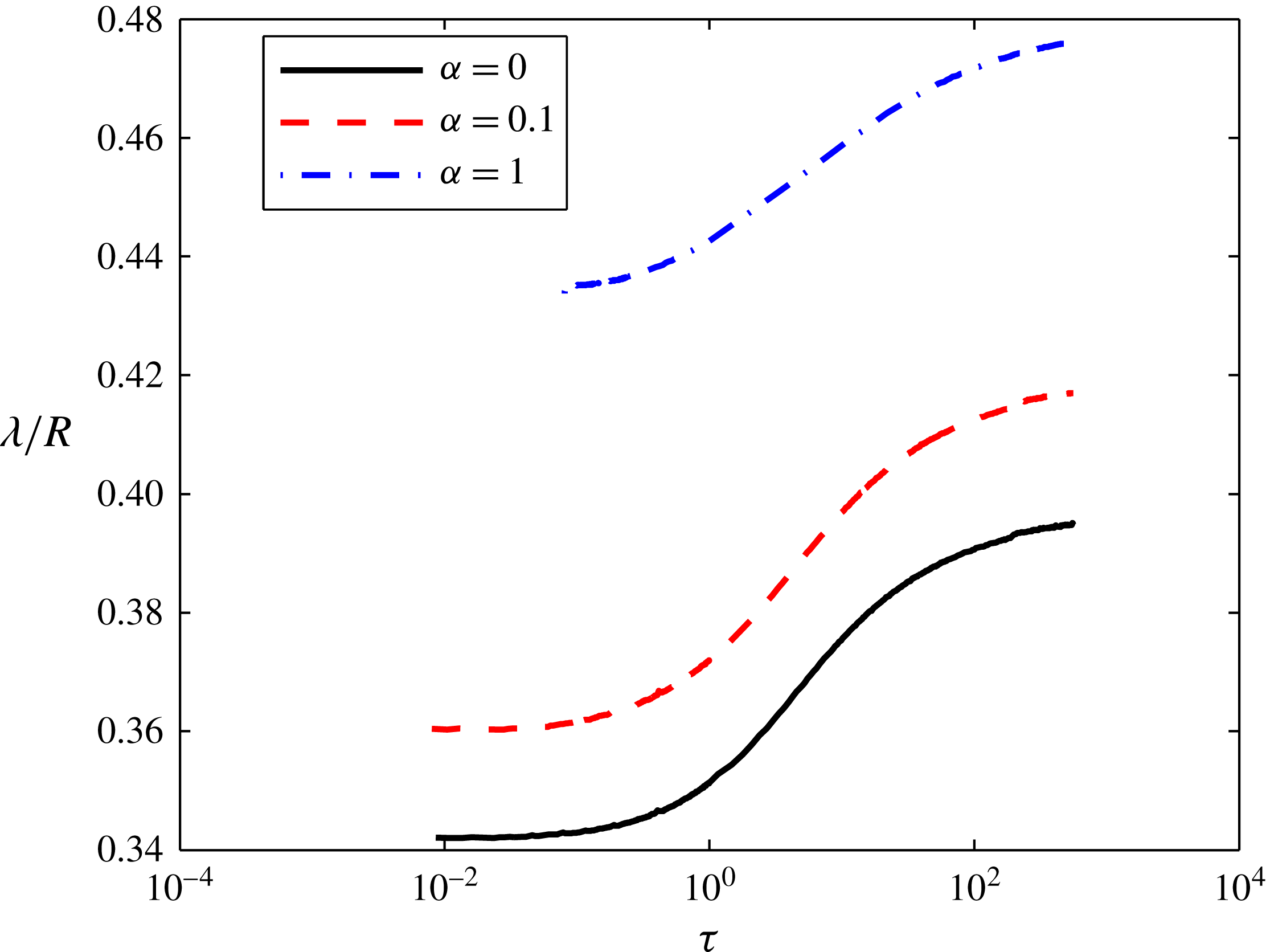
Finally, to calculate the permeability profile of the rock, one needs information about the three characteristic parameters given by (4.8)–(4.10). Equation (5.5) and the probability distribution of the recorded microseismic events provide two relations. The third relation can be the measurement of the temporal injection pressure profile,
 $P_{inj}$
, since
 $P_{inj}$
is given by:
 $$\begin{eqnarray}P_{inj}(R_{w},t)=\frac{P_{ch}}{t_{ch}^{\unicode[STIX]{x1D6FF}}}\left[(\unicode[STIX]{x1D716}+1)\ln \left(\frac{R}{R_{w}\unicode[STIX]{x1D702}_{max}}\right)\right]^{1/(\unicode[STIX]{x1D716}+1)}t^{\unicode[STIX]{x1D6FF}},\end{eqnarray}$$
where
 $R_{w}$
is the well radius.
6 Summary and conclusion
The interplay between fluid transport through a continuum fractured porous medium, fluid seepage through a permeable matrix and the evolution of the medium’s porosity was modelled. The model circumvents the difficulties of simulating the fracturing process of realistic weak plane networks and provides information about the connectivity of the activated fractures and the propagation rate of the network. The fracturing fluid was assumed to flow through a cluster of activated fractures and, as it advances, the cluster evolves. Fluid flow was described by Darcy’s equation where the permeability and porosity of the network of activated fractures evolve spatially and temporally. Percolation theory was employed to derive constitutive relations that correlate the permeability and porosity of the activated fracture cluster with fluid pressure based on the assumption that each fracture is activated when the invading fluid pressure reaches a critical value. The use of percolation theory is applicable when a characteristic correlation length is much smaller than the radius of the activated cluster and much larger than the average spacing of the pre-existing fractures.
The transport equation of the fracturing fluid has been derived for a time-dependent injection rate,
 $Q_{0}t^{\unicode[STIX]{x1D6FC}}$
in a two-dimensional network. In two distinct regimes, the fluid front was shown to grow as a power law of time and the structure of the activated fracture cluster to evolve in a self-similar fashion. The first regime arises when enough fractures are activated to form a continuum medium through which the fracturing fluid flows but the cluster is not large enough to lose a significant amount of the fracturing fluid through leak off. The other self-similar regime arises when the surface area of the activated fractures is large enough such that most of the injected fluid leaks into the matrix. The network properties in the two regimes are summarized in table 2. The cross-over time at which the leakage rate starts to play a role in slowing down the cluster growth rate depends primarily on the permeability and porosity of the rock matrix, the threshold fracture critical pressure and the viscosity of the fluid. The dependence of the cross-over time on these parameters is given by (4.8).
When the leakage is negligible, it has been shown that given the same volume of injected fracturing fluid over the same fracturing process duration, injecting the fluid at a constant rate gives a larger stimulated volume when compared to ramping up the injection rate. On the other hand, the number density and permeability is larger when the injection rate is increasing with time. Also, in this regime, decreasing the injection rate or the fracturing fluid viscosity gives a larger stimulated volume with a smaller number density of activated fractures for the same total injected fluid volume. The physical explanation for this behaviour is that increasing the injection rate,
 $Q_{0}t^{\unicode[STIX]{x1D6FC}}$
, or the fluid viscosity increases the viscous pressure drop which, in turn, increases the number density of fractures near the injection well. Thereby, the fluid available to extend the activated cluster is reduced. Therefore, for ultra-low permeability shale formations, it is recommended to perform the fracturing at a low constant injection rate with low viscosity. This would give a larger stimulated volume and hence a larger region of accessible natural gas.
On the other hand, in the leakage dominant regime, increasing the fracturing fluid viscosity or
 $\unicode[STIX]{x1D6FC}$
gives a larger stimulated volume and number density of activated fractures given the same amount of injected fluid over a certain fracturing period. Increasing the viscosity decreases the leakage rate per surface area and therefore more fluid is used to extend the activated cluster and increasing
 $\unicode[STIX]{x1D6FC}$
provides a larger amount of available fluid to extend the cluster. As a result of this analysis, the optimum fracturing strategy for relatively high permeability shale formations is to ramp up the injection rate of a high viscosity fluid.
To analyse the relative density of the network via measurable parameters, a probability distribution function of recorded microseismic activities (or fracture activation events),
 $g(r,t)$
, was derived. The region where ninety per cent of the probable microseismic events are located has been found to be near the edge of the cluster. The thickness of this region when compared to the cluster radius has been shown to increase as leakage starts to become significant. Increasing the value of
 $\unicode[STIX]{x1D6FC}$
was shown to increase the thickness of this region due to the increase in pressure drop required to drive the flow.
The model developed in this paper is valid for moderate injection rates and fluid viscosities for which a characteristic correlation length is much larger than the average spacing of the fractures. In this model, fluid inertia, which might be important for very large flow rates and low fluid viscosity, is neglected. For extremely viscous fluids, the characteristic correlation length can be of the same order of magnitude as the average fracture length. In this case, a model in which the bulk of the cluster has a constant permeability but there is a percolating front with evolving permeability can be used. For a more complete understanding of the fracturing process, one would need to incorporate a model of how the solid matrix stress perturbations generated by the activation of fractures affect the critical pressure of the fractures and thereby the growth of the cluster.
Acknowledgements
The authors would like to thank F. Escobedo, K. Quinn, J. Sethna, A. Zehnder and A. Roy for helpful discussions. We would also like to thank an anonymous referee for suggesting a simple method to solve the system of equations described in appendix B. The Research and Development Center of Saudi Aramco provided funding for M.G.A. through the Advanced Degree Program. D.L.K. received support from NSF CBET grant 1505795.
Appendix A. Single fracture analytical solution and its range of validity
In this section, we show how (3.16) can be solved analytically when
 $\unicode[STIX]{x1D6E5}_{pc}=0$
and the physical conditions in dimensional variables for which this is limiting case is valid.
When
 $\unicode[STIX]{x1D6E5}_{pc}=0$
, equation (3.20) can be rewritten as:
 $$\begin{eqnarray}\frac{\text{d}\bar{L}}{\text{d}\bar{t}}=1-\int _{0}^{\bar{t}}\sqrt{\frac{1}{\bar{t}-\bar{t^{\prime }}}}\frac{\text{d}\bar{x}}{\text{d}\bar{t^{\prime }}}\,\text{d}\bar{t^{\prime }}.\end{eqnarray}$$
Using Laplace transform and the initial condition that the initial length is zero, one can get:
 $$\begin{eqnarray}F(s)=\frac{1}{s}\left(\frac{1}{s+\sqrt{\unicode[STIX]{x03C0}s}}\right)=\frac{1}{s^{3/2}}\left(\frac{\sqrt{s}-\sqrt{\unicode[STIX]{x03C0}}}{s-\unicode[STIX]{x03C0}}\right).\end{eqnarray}$$
By using partial fraction decomposition, equation (A 2) can be rewritten as:
 $$\begin{eqnarray}F(s)=\frac{1}{\sqrt{\unicode[STIX]{x03C0}}s^{3/2}}+\frac{1}{\unicode[STIX]{x03C0}\sqrt{s}(\sqrt{s}+\sqrt{\unicode[STIX]{x03C0}})}-\frac{1}{\unicode[STIX]{x03C0}s}.\end{eqnarray}$$
Knowing that
 ${\mathcal{L}}_{s}^{-1}\{s^{-3/2}\}=2\sqrt{\bar{t}}/\sqrt{\unicode[STIX]{x03C0}}$
,
 ${\mathcal{L}}_{s}^{-1}\{1/(\sqrt{s}(\sqrt{s}+\sqrt{\unicode[STIX]{x03C0}}))\}=\text{e}^{\unicode[STIX]{x03C0}\bar{t}}\text{erfc}(\sqrt{\unicode[STIX]{x03C0}\bar{t}})$
, and
 ${\mathcal{L}}_{s}^{-1}\{s\}=1$
, the length of the fracture can be given by:
 $$\begin{eqnarray}\bar{L}=\frac{1}{\unicode[STIX]{x03C0}}[\text{e}^{\unicode[STIX]{x03C0}\bar{t}}\text{erfc}(\sqrt{\unicode[STIX]{x03C0}\bar{t}})+2\sqrt{\bar{t}}-1].\end{eqnarray}$$
The assumptions of the unidirectional leakage flow and negligible viscous effects on the leakage that led to the above analytical solution are valid when (3.21) applies. Using a unidirectional flow and neglecting the effects of the viscous pressure drop on the leakage velocity led to a simple coupling between the leakage rate and the fracture growth rate, i.e.
 $v_{l}\approx \sqrt{(k_{m}\unicode[STIX]{x1D700}_{m}(P_{c}-P_{f}))/(2\unicode[STIX]{x1D707}(t-t^{\prime }))}$
, that was used to obtain the analytical solution.
The unidirectional flow of the leaking fluid is only valid when the leakage velocity is much smaller than the fracture propagation velocity,
 $\text{d}L/\text{d}t$
. Since the leakage velocity decays as
 $1/\sqrt{t-t^{\prime }}$
, the unidirectional assumption is expected to be violated near the fracture tip where the leakage velocity is large. The thickness,
 $\unicode[STIX]{x1D706}_{le}$
, of the region where the leakage velocity is greater than the fracture growth rate can be obtained by finding the distance away from the fluid front at which the leakage velocity is equal to
 $\text{d}L/\text{d}t$
. In order for the region with high leakage velocity to be localized,
 $\unicode[STIX]{x1D706}_{le}\ll L$
. Since, the fracture’s growth rate changes with time, we will analyse the behaviour of
 $\unicode[STIX]{x1D706}_{le}/L$
at early times and when the leakage dominates the growth.
At the beginning of the fracture growth, the fracture length increases at a constant rate,
 $Q/bw$
. Therefore, the thickness can be found by simply equating the leakage velocity with the constant flow rate and the criterion for unidirectional leakage in the short-time regime to be valid can be written as:
 $$\begin{eqnarray}\frac{bwk_{m}\unicode[STIX]{x1D700}_{m}(P_{c}-P_{f})}{2Q\unicode[STIX]{x1D707}}\ll L(t).\end{eqnarray}$$
In the long-time regime, on the other hand,
 $\text{d}L/\text{d}t=Q/(2\unicode[STIX]{x03C0}wC\sqrt{P_{c}-P_{f}}\sqrt{t})$
and thereby to find
 $\unicode[STIX]{x1D706}_{le}$
, one can write:
 $$\begin{eqnarray}\frac{1}{\sqrt{L^{2}-(L-\unicode[STIX]{x1D706}_{le})^{2}}}=\frac{Q}{2\unicode[STIX]{x03C0}wC^{2}(P_{c}-P_{f})L}.\end{eqnarray}$$
Since
 $\unicode[STIX]{x1D706}_{le}\ll L$
, the term on the left-hand side of (A 6) can be approximated as
 $1/\sqrt{\unicode[STIX]{x1D706}_{le}L}$
. Therefore, the assumption of unidirectional leakage flow is valid in the long-time regime when:
 $$\begin{eqnarray}\frac{Q}{w}\unicode[STIX]{x1D707}\gg k_{m}\unicode[STIX]{x1D700}_{m}(P_{c}-P_{f}).\end{eqnarray}$$
The other simplification, which consists of neglecting the effects of the viscous pressure drop on the leakage velocity, applies for both time regimes when
 $\unicode[STIX]{x1D6E5}_{pc}\ll 1$
. From the definition of
 $\unicode[STIX]{x1D6E5}_{pc}$
, one can derive the following criterion for which the effects of the pressure variation on the leakage velocity are negligible:
 $$\begin{eqnarray}\frac{Q}{w}\unicode[STIX]{x1D707}\ll (P_{c}-P_{f})b\sqrt{k_{m}\unicode[STIX]{x1D700}_{m}}.\end{eqnarray}$$
To sum up, the simplified leakage velocity can be used when (A 8) along with (A 5), and (A 8) and (A 7) are satisfied simultaneously in the short- and long-time regimes, respectively. At early time, merging the two criteria yields:
 $$\begin{eqnarray}\frac{b}{L(t)}\ll \frac{\displaystyle \left(\frac{Q}{wb}\right)}{\displaystyle \left(\frac{(P_{c}-P_{f})k_{m}\unicode[STIX]{x1D700}_{m}}{\unicode[STIX]{x1D707}b}\right)}\ll \frac{b}{\sqrt{k_{m}\unicode[STIX]{x1D700}_{m}}}\end{eqnarray}$$
and for the long-time regime yields:
 $$\begin{eqnarray}1\ll \frac{\displaystyle \left(\frac{Q}{wb}\right)}{\displaystyle \left(\frac{(P_{c}-P_{f})k_{m}\unicode[STIX]{x1D700}_{m}}{\unicode[STIX]{x1D707}b}\right)}\ll \frac{b}{\sqrt{k_{m}\unicode[STIX]{x1D700}_{m}}}.\end{eqnarray}$$
One can see that since
 $b$
is a few millimetres, one only needs to satisfy (A 10) in order to use the analytical solution for the fracture growth. In formations with a permeability of
 $10^{-16}~\text{m}^{2}$
such as tight gas reservoirs, a critical formation pressure of the order of MPa, and an aperture of the order of a millimetre, this criterion is satisfied when a low viscosity fluid such as water is injected at flow rates per width smaller than
 $10^{-3}~\text{m}^{2}~\text{s}^{-1}$
. As the fluid’s viscosity increases, the flow rate per width needed to satisfy the criterion decreases. For shale gas rocks where the permeability ranges from
 $10^{-21}~\text{m}^{2}$
to
 $10^{-18}~\text{m}^{2}$
, the flow rates per width up to which one will be able to use both unidirectional flow and negligible pressure drop assumptions range from
 $10^{-5}~\text{m}^{2}~\text{s}^{-1}$
to
 $10^{-4}~\text{m}^{2}~\text{s}^{-1}$
for water.
Appendix B. Long-time similarity solution when
 $t^{\prime }=f(s,r)$

In § 4.3, it has been mentioned that solving (4.11) numerically is difficult and thus, we have simplified the equations by neglecting the dependence of the leakage velocity on the time at which a fracture is activated. Moreover, we showed that the simplification preserves the same scalings but over-predicts the rate at which the cluster grows in the long time regime. In this section, we derive the integro-differential equation for the long-time regime when the leakage rate is kept as in (4.11) and describe the method used to solve it.
The integro-differential equations that govern the growth behaviour of the cluster is written as:
 $$\begin{eqnarray}\displaystyle & \displaystyle \frac{\unicode[STIX]{x2202}p^{\unicode[STIX]{x1D6FD}}}{\unicode[STIX]{x2202}\unicode[STIX]{x1D70F}}=\frac{1}{\unicode[STIX]{x1D70C}}\frac{\unicode[STIX]{x2202}}{\unicode[STIX]{x2202}\unicode[STIX]{x1D70C}}\left(\unicode[STIX]{x1D70C}p^{\unicode[STIX]{x1D716}}\frac{\unicode[STIX]{x2202}p}{\unicode[STIX]{x2202}\unicode[STIX]{x1D70C}}\right)-\unicode[STIX]{x1D6FD}\int _{0}^{p}\frac{\unicode[STIX]{x1D701}^{\unicode[STIX]{x1D6FD}-1}}{\sqrt{\unicode[STIX]{x1D70F}-\unicode[STIX]{x1D70F}^{\prime }}}\,\text{d}\unicode[STIX]{x1D701}, & \displaystyle\end{eqnarray}$$
 $$\begin{eqnarray}\displaystyle & \displaystyle \frac{\unicode[STIX]{x2202}}{\unicode[STIX]{x2202}\unicode[STIX]{x1D70F}}\left(\int _{0}^{\unicode[STIX]{x1D70C}_{max}}p^{\unicode[STIX]{x1D6FD}}\unicode[STIX]{x1D70C}\,\text{d}\unicode[STIX]{x1D70C}\right)=\unicode[STIX]{x1D70F}^{\unicode[STIX]{x1D6FC}}-\unicode[STIX]{x1D6FD}\int _{0}^{\unicode[STIX]{x1D70C}_{max}}\,\text{d}\unicode[STIX]{x1D701}\int _{0}^{p}\frac{\unicode[STIX]{x1D701}^{\unicode[STIX]{x1D6FD}-1}}{\sqrt{\unicode[STIX]{x1D70F}-\unicode[STIX]{x1D70F}^{\prime }}}\unicode[STIX]{x1D70C}\,\text{d}\unicode[STIX]{x1D70C}. & \displaystyle\end{eqnarray}$$
To obtain the similarity solution, let
 $\unicode[STIX]{x1D702}=\unicode[STIX]{x1D70C}\unicode[STIX]{x1D70F}^{-\unicode[STIX]{x1D6FE}_{l}}$
and:
 $$\begin{eqnarray}\unicode[STIX]{x1D719}=p\unicode[STIX]{x1D70F}^{-\unicode[STIX]{x1D6FF}_{l}},\end{eqnarray}$$
where
 $\unicode[STIX]{x1D6FE}_{l}$
and
 $\unicode[STIX]{x1D6FF}_{l}$
are the same scaling exponents used in § 4.3 and their values are given in table 1. To scale the leakage term in (B 1), one must account for both the direct
 $\unicode[STIX]{x1D70F}$
dependence and the dependence of
 $p$
on
 $\unicode[STIX]{x1D70F}$
. Therefore, let
 $\unicode[STIX]{x1D701}=\unicode[STIX]{x1D719}(\unicode[STIX]{x1D702}^{\prime })\unicode[STIX]{x1D70F}^{\prime \unicode[STIX]{x1D6FF}_{l}}$
where
 $\unicode[STIX]{x1D702}^{\prime }=\unicode[STIX]{x1D70C}\unicode[STIX]{x1D70F}^{\prime -\unicode[STIX]{x1D6FE}_{l}}$
. Then,
 $$\begin{eqnarray}\text{d}\unicode[STIX]{x1D701}=\unicode[STIX]{x1D70F}^{\prime \unicode[STIX]{x1D6FF}_{l}-1}\left(\unicode[STIX]{x1D6FF}_{l}\unicode[STIX]{x1D719}(\unicode[STIX]{x1D702}^{\prime })-\unicode[STIX]{x1D6FE}_{l}\unicode[STIX]{x1D702}^{\prime }\frac{\text{d}\unicode[STIX]{x1D719}(\unicode[STIX]{x1D702}^{\prime })}{\text{d}\unicode[STIX]{x1D702}^{\prime }}\right)\,\text{d}\unicode[STIX]{x1D70F}^{\prime }.\end{eqnarray}$$
Since
 $\unicode[STIX]{x1D701}=0$
when
 $\unicode[STIX]{x1D70C}=\unicode[STIX]{x1D70C}_{max}$
and
 $\unicode[STIX]{x1D701}=p$
when
 $\unicode[STIX]{x1D70F}^{\prime }=\unicode[STIX]{x1D70F}$
:
 $$\begin{eqnarray}\int _{0}^{p}\frac{\unicode[STIX]{x1D701}^{\unicode[STIX]{x1D6FD}-1}}{\sqrt{\unicode[STIX]{x1D70F}-\unicode[STIX]{x1D70F}^{\prime }}}\,\text{d}\unicode[STIX]{x1D701}=\unicode[STIX]{x1D70F}^{\unicode[STIX]{x1D6FD}\unicode[STIX]{x1D6FF}_{l}-1/2}\int _{(\unicode[STIX]{x1D702}/\unicode[STIX]{x1D702}_{max})^{1/\unicode[STIX]{x1D6FE}_{l}}}^{1}\,\text{d}\unicode[STIX]{x1D6F6}\frac{\unicode[STIX]{x1D6F6}^{\unicode[STIX]{x1D6FD}\unicode[STIX]{x1D6FF}_{l}-1}}{\sqrt{1-\unicode[STIX]{x1D6F6}}}\unicode[STIX]{x1D719}(\unicode[STIX]{x1D702}^{\prime })^{\unicode[STIX]{x1D6FD}-1}\left(\unicode[STIX]{x1D6FF}_{l}\unicode[STIX]{x1D719}(\unicode[STIX]{x1D702}^{\prime })-\unicode[STIX]{x1D6FE}_{l}\unicode[STIX]{x1D702}^{\prime }\frac{\text{d}\unicode[STIX]{x1D719}(\unicode[STIX]{x1D702}^{\prime })}{\text{d}\unicode[STIX]{x1D702}^{\prime }}\right),\end{eqnarray}$$
where
 $\unicode[STIX]{x1D702}^{\prime }$
can be rewritten as
 $\unicode[STIX]{x1D702}^{\prime }=\unicode[STIX]{x1D702}\unicode[STIX]{x1D6F6}^{-\unicode[STIX]{x1D6FE}_{l}}$
and
 $\unicode[STIX]{x1D6F6}=\unicode[STIX]{x1D70F}^{\prime }/\unicode[STIX]{x1D70F}$
.
Now, when substituting (B 5) along with the scaled variables into (4.11)–(4.14) and neglecting the left-hand terms, the desired ordinary integro-differential equations are given by:
 $$\begin{eqnarray}\displaystyle & \displaystyle \frac{1}{\unicode[STIX]{x1D702}}\frac{\text{d}}{\text{d}\unicode[STIX]{x1D702}}\left(\unicode[STIX]{x1D702}\unicode[STIX]{x1D719}^{\unicode[STIX]{x1D716}}\frac{\text{d}\unicode[STIX]{x1D719}}{\text{d}\unicode[STIX]{x1D702}}\right)=\unicode[STIX]{x1D6FD}\int _{(\unicode[STIX]{x1D702}/\unicode[STIX]{x1D702}_{max}^{l})^{1/\unicode[STIX]{x1D6FE}_{l}}}^{1}\,\text{d}\unicode[STIX]{x1D6F6}\frac{\unicode[STIX]{x1D6F6}^{\unicode[STIX]{x1D6FD}\unicode[STIX]{x1D6FF}_{l}-1}}{\sqrt{1-\unicode[STIX]{x1D6F6}}}\unicode[STIX]{x1D719}(\unicode[STIX]{x1D702}^{\prime })^{\unicode[STIX]{x1D6FD}-1}\left(\unicode[STIX]{x1D6FF}_{l}\unicode[STIX]{x1D719}(\unicode[STIX]{x1D702}^{\prime })-\unicode[STIX]{x1D6FE}_{l}\unicode[STIX]{x1D702}^{\prime }\frac{\text{d}\unicode[STIX]{x1D719}(\unicode[STIX]{x1D702}^{\prime })}{\text{d}\unicode[STIX]{x1D702}^{\prime }}\right),\quad & \displaystyle\end{eqnarray}$$
 $$\begin{eqnarray}\displaystyle & \displaystyle 1=\unicode[STIX]{x1D6FD}\int _{0}^{\unicode[STIX]{x1D702}_{max}^{l}}\,\text{d}\unicode[STIX]{x1D702}\int _{(\unicode[STIX]{x1D702}/\unicode[STIX]{x1D702}_{max}^{l})^{1/\unicode[STIX]{x1D6FE}_{l}}}^{1}\,\text{d}\unicode[STIX]{x1D6F6}\frac{\unicode[STIX]{x1D6F6}^{\unicode[STIX]{x1D6FD}\unicode[STIX]{x1D6FF}_{l}-1}}{\sqrt{1-\unicode[STIX]{x1D6F6}}}\unicode[STIX]{x1D719}(\unicode[STIX]{x1D702}^{\prime })^{\unicode[STIX]{x1D6FD}-1}\left(\unicode[STIX]{x1D6FF}_{l}\unicode[STIX]{x1D719}(\unicode[STIX]{x1D702}^{\prime })-\unicode[STIX]{x1D6FE}_{l}\unicode[STIX]{x1D702}^{\prime }\frac{\text{d}\unicode[STIX]{x1D719}(\unicode[STIX]{x1D702}^{\prime })}{\text{d}\unicode[STIX]{x1D702}^{\prime }}\right)\unicode[STIX]{x1D702}, & \displaystyle\end{eqnarray}$$
 $$\begin{eqnarray}\displaystyle & \displaystyle \unicode[STIX]{x1D719}=0,\quad \text{on }\unicode[STIX]{x1D702}=\unicode[STIX]{x1D702}_{max}^{l}, & \displaystyle\end{eqnarray}$$
 $$\begin{eqnarray}\displaystyle & \displaystyle \lim _{\unicode[STIX]{x1D702}\rightarrow ~0}\unicode[STIX]{x1D702}\unicode[STIX]{x1D719}^{\unicode[STIX]{x1D716}}\frac{\text{d}\unicode[STIX]{x1D719}}{\text{d}\unicode[STIX]{x1D702}}=-1. & \displaystyle\end{eqnarray}$$
The asymptotic solution of
 $\unicode[STIX]{x1D719}$
near the injection well is given by (4.22) while the behaviour of
 $\unicode[STIX]{x1D719}$
as
 $\unicode[STIX]{x1D702}\rightarrow \unicode[STIX]{x1D702}_{max}^{l}$
is given by:
 $$\begin{eqnarray}\unicode[STIX]{x1D719}=\left[\frac{\{(\unicode[STIX]{x1D716}+1)\unicode[STIX]{x1D6FA}-1\}\unicode[STIX]{x1D6E4}(\unicode[STIX]{x1D6FD}\unicode[STIX]{x1D6FA}+1)}{\unicode[STIX]{x1D6E4}(\unicode[STIX]{x1D6FD}\unicode[STIX]{x1D6FA})\sqrt{\unicode[STIX]{x03C0}}\unicode[STIX]{x1D6FD}(\unicode[STIX]{x1D6FE}_{l}\unicode[STIX]{x1D702}_{max}^{l})^{2}}\right]^{1/(\unicode[STIX]{x1D6FD}-\unicode[STIX]{x1D716}-1)}\left[1-\left(\frac{\unicode[STIX]{x1D702}}{\unicode[STIX]{x1D702}_{max}^{l}}\right)^{1/\unicode[STIX]{x1D6FE}_{l}}\right]^{\unicode[STIX]{x1D6FA}},\end{eqnarray}$$
where
 $\unicode[STIX]{x1D6FA}=3/(2(\unicode[STIX]{x1D716}+1-\unicode[STIX]{x1D6FD}))$
and
 $\unicode[STIX]{x1D6E4}(x)$
is the complete gamma function. As one expects, the assumption of simplifying the leakage rate does not change the qualitative behaviour of
 $\unicode[STIX]{x1D719}$
. Both asymptotic solutions, when the leakage is simplified and when the full form is used, have the same power law exponent but with a different prefactor.
To solve the system of equations, equations (B 6) and (B 7) were decoupled by scaling
 $\unicode[STIX]{x1D719}$
with
 $(\unicode[STIX]{x1D702}_{max}^{l})^{2/(\unicode[STIX]{x1D6FD}-\unicode[STIX]{x1D716}-1)}$
and
 $\unicode[STIX]{x1D702}$
with
 $\unicode[STIX]{x1D702}_{max}^{l}$
. Following the procedure described in (Gelmi & Jorquera Reference Gelmi and Jorquera2014), equation (B 6) was integrated to obtain the profile of the scaled
 $\unicode[STIX]{x1D719}$
and the value of
 $\unicode[STIX]{x1D702}_{max}^{l}$
was calculated using (B 7). The two boundary conditions needed to integrate (B 6) were derived from (B 10).
Appendix C. Numerical schemes
In this section, we will describe the numerical scheme that has been used to solve the ordinary differential equations in the self-similar regimes and the simplified partial differential equation.
To solve for the self-similar pressure profile in the short-time similarity regime, equation (4.18), a shooting method was used. To start integrating the equations, the flux within a small region with a radius of
 $10^{-8}$
from the injection point is assumed to be constant,
 $C_{q}$
. The value of
 $C_{q}$
is unknown and it is determined by an iteration method. Then, the integration using the values of
 $\unicode[STIX]{x1D719}$
and
 $\text{d}\unicode[STIX]{x1D719}/\text{d}\unicode[STIX]{x1D702}$
given
 $C_{q}$
is carried out. Equation (4.20) is used as a criterion to stop integrating the equations. The value of
 $C_{q}$
is adjusted until (4.19) is satisfied.
The long-time ordinary differential equation and the full partial differential equations were solved using a finite difference method. In both methods, the spatial variable was scaled before discretizing the terms. When solving the partial differential equation, one needs to keep track of the boundary at the cluster’s edge that moves with time. By scaling the position variable with the cluster’s radius, one can discretize the equations on a well-defined region that ranges from 0 to 1. Similarly, the value of
 $\unicode[STIX]{x1D702}_{max}$
is unknown. By rescaling the spatial variable
 $\unicode[STIX]{x1D702}$
with
 $\unicode[STIX]{x1D702}_{max}$
, one can perform discretization for a defined region between 0 and 1.
Below is a description for the method used to solve the partial differential equation. Adapting this method to solve for the long-time regime, one can replace
 $R$
by
 $\unicode[STIX]{x1D702}_{max}$
and follow the same discretization approach. For a
 $D$
-dimensional network, let
 $X=r/R$
such that
 $P=f(t,X)$
. Hence, equations (4.27) and (4.28) become:
 $$\begin{eqnarray}\displaystyle & \displaystyle \frac{\unicode[STIX]{x2202}P}{\unicode[STIX]{x2202}t}=\frac{X}{R}\left(\frac{\text{d}R}{\text{d}t}\right)\frac{\unicode[STIX]{x2202}P}{\unicode[STIX]{x2202}X}+\frac{P^{1-\unicode[STIX]{x1D6FD}}}{\unicode[STIX]{x1D6FD}X^{D-1}R^{2}}\frac{\unicode[STIX]{x2202}}{\unicode[STIX]{x2202}X}\left(X^{D-1}P^{\unicode[STIX]{x1D716}}\frac{\unicode[STIX]{x2202}P}{\unicode[STIX]{x2202}X}\right)-\frac{P}{\unicode[STIX]{x1D6FD}\sqrt{t-t^{\prime }}}, & \displaystyle\end{eqnarray}$$
 $$\begin{eqnarray}\displaystyle & \displaystyle \frac{\unicode[STIX]{x2202}}{\unicode[STIX]{x2202}t}\left(R^{D}\int _{0}^{1}P^{\unicode[STIX]{x1D6FD}}X^{D-1}\,\text{d}X\right)=t^{\unicode[STIX]{x1D6FC}}-R^{D}\int _{0}^{1}P^{\unicode[STIX]{x1D6FD}}\frac{X^{D-1}}{\sqrt{t-t^{\prime }}}\,\text{d}X. & \displaystyle\end{eqnarray}$$
Introducing
 $X_{i}=(i-1/2)\unicode[STIX]{x0394}X$
and a time step
 $\text{d}t$
, equation (C 1) can be discretized as
 $$\begin{eqnarray}\frac{P_{i}^{n+1}-P_{i}^{n}}{\text{d}t}=\frac{1}{2}(T_{i}^{n}+F_{i}^{n}+L_{i}^{n}+T_{i}^{n+1}+F_{i}^{n+1}+L_{i}^{n+1}),\end{eqnarray}$$
where
 $$\begin{eqnarray}\displaystyle & \displaystyle T_{i}^{n}=\frac{X_{i}}{R^{n}}\left(\frac{R^{n}-R^{n-1}}{\text{d}t}\right)\frac{P_{i+1}^{n}-P_{i-1}^{n}}{X_{i+1}-X_{i-1}}, & \displaystyle\end{eqnarray}$$
 $$\begin{eqnarray}\displaystyle & \displaystyle F_{i}^{n}=\frac{(P_{i}^{n})^{1-\unicode[STIX]{x1D6FD}}}{X_{i}^{D-1}\unicode[STIX]{x1D6FD}(R^{n})^{2}}\left[\frac{\displaystyle X_{i+1/2}^{D-1}\left(\frac{P_{i+1}^{n}-P_{i}^{n}}{\unicode[STIX]{x0394}X}\right)\unicode[STIX]{x1D713}_{i+1/2}^{n+1/2}-X_{i-1/2}^{D-1}\left(\frac{P_{i}^{n}-P_{i-1}^{n}}{\unicode[STIX]{x0394}X}\right)\unicode[STIX]{x1D713}_{i-1/2}^{n+1/2}}{\unicode[STIX]{x0394}X}\right]\!,\quad & \displaystyle\end{eqnarray}$$
 $$\begin{eqnarray}\displaystyle & \displaystyle L_{i}^{n}=\frac{P_{i}^{n}}{\unicode[STIX]{x1D6FD}\sqrt{t^{n}-t_{i}^{^{\prime }n}}}, & \displaystyle\end{eqnarray}$$
 $$\begin{eqnarray}\displaystyle & \displaystyle \unicode[STIX]{x1D713}_{i+1/2}^{n+1/2}={\textstyle \frac{1}{4}}[(P_{i+1}^{n+1})^{\unicode[STIX]{x1D716}}+(P_{i}^{n+1})^{\unicode[STIX]{x1D716}}+(P_{i+1}^{n})^{\unicode[STIX]{x1D716}}+(P_{i}^{n})^{\unicode[STIX]{x1D716}}].\quad & \displaystyle\end{eqnarray}$$
Similarly, the boundary conditions can be expressed as:
 $$\begin{eqnarray}\left.\begin{array}{@{}c@{}}\displaystyle P_{1}^{n+1}=P_{2}^{n+1}+\frac{(t^{n+1})^{\unicode[STIX]{x1D6FC}}\unicode[STIX]{x0394}X}{X_{1}^{D-1}(P_{1}^{n+1})^{\unicode[STIX]{x1D716}}},\\ P_{N}^{n+1}=0.\end{array}\right\}\end{eqnarray}$$
To find the cluster radius in a time step
 $n+1$
, equation (C 2) is discretized and solved for
 $R^{n+1}$
such that:
 $$\begin{eqnarray}R^{n+1}=\left[\frac{1/2[(t^{n+1})^{\unicode[STIX]{x1D6FC}}+(t^{n})^{\unicode[STIX]{x1D6FC}}]\,\text{d}t+(R^{n})^{D}I^{n}}{I^{n+1}}\right]^{1/D},\end{eqnarray}$$
where
 $$\begin{eqnarray}I^{n}=\int _{0}^{1}P^{\unicode[STIX]{x1D6FD}}\left(1-\frac{\text{d}t}{2\sqrt{t^{n}-(t^{\prime })^{n}}}\right)X^{D-1}\,\text{d}X.\end{eqnarray}$$
 $t^{\prime }$
is a function of time because the nodes in computational space correspond to different points in space as the cluster grows. To estimate
 $t^{\prime }$
at the time step
 $n+1$
, we use a Taylor series expansion that includes a finite difference approximation of the rate at which each node moves:
 $$\begin{eqnarray}(t_{i}^{\prime })^{n+1}=(t_{i}^{\prime })^{n}+\frac{[(t_{i}^{\prime })^{n}-(t_{i}^{\prime })^{n-1}](R^{n+1}-R^{n})}{R^{n}-R^{n-1}}.\end{eqnarray}$$
The initial pressure is estimated by neglecting the leakage and as
 $R\rightarrow 0$
, the storage term is neglected. Thus, the flux is assumed to be independent of
 $r$
within
 $r<R_{init}$
so that
 $$\begin{eqnarray}P(t_{init},X)=\left[t^{\unicode[STIX]{x1D6FC}}(\unicode[STIX]{x1D716}+1)\ln \left(\frac{1}{X}\right)\right]^{1/(\unicode[STIX]{x1D716}+1)}\end{eqnarray}$$
and
 $$\begin{eqnarray}R_{init}=\left[\frac{2^{(\unicode[STIX]{x1D6FD}/(1+\unicode[STIX]{x1D716}))+1}(\unicode[STIX]{x1D716}+1)^{-\unicode[STIX]{x1D6FD}/(1+\unicode[STIX]{x1D716})}}{\displaystyle (1+\unicode[STIX]{x1D6FC})\unicode[STIX]{x1D6E4}\left(\frac{\unicode[STIX]{x1D6FD}}{1+\unicode[STIX]{x1D716}}+1\right)}\right]^{1/2}t_{init}^{(\unicode[STIX]{x1D6FC}/2)(1-(\unicode[STIX]{x1D6FD}/(1+\unicode[STIX]{x1D716})))+1/2},\end{eqnarray}$$
where
 $\unicode[STIX]{x1D6E4}(x)$
is the complete gamma function. In three dimensions, the initial pressure and cluster growth rate are estimated via:
 $$\begin{eqnarray}\displaystyle & \displaystyle P(t_{init},X)=\left[t^{\unicode[STIX]{x1D6FC}}(\unicode[STIX]{x1D716}+1)\left(\frac{1}{X}-1\right)\right]^{1/(\unicode[STIX]{x1D716}+1)}, & \displaystyle\end{eqnarray}$$
 $$\begin{eqnarray}\displaystyle & \displaystyle R_{init}=\left[(1+\unicode[STIX]{x1D6FC})\int _{0}^{1}X^{2}\left(\frac{1}{X}-1\right)^{\unicode[STIX]{x1D6FD}/(1+\unicode[STIX]{x1D716})}\,\text{d}X\right]^{-1/3}(\unicode[STIX]{x1D716}+1)^{-\unicode[STIX]{x1D6FD}/(3(1+\unicode[STIX]{x1D716}))}t_{init}^{(\unicode[STIX]{x1D6FC}/3)(1-(\unicode[STIX]{x1D6FD}/(1+\unicode[STIX]{x1D716})))+1/3}. & \displaystyle \nonumber\\ \displaystyle & & \displaystyle\end{eqnarray}$$
The above mentioned method can be easily adapted to solve for
 $\unicode[STIX]{x1D719}$
in the long-time regime. One can start with (4.30) and follow the same described discretization procedure. To find
 $\unicode[STIX]{x1D702}_{max}^{l}$
, one can use (4.31) instead of (C 2).
Appendix D. Validity of primary model assumptions
In this section, the range of validity of several assumptions required for the model formulation is discussed. First, we will consider when the effects of buoyancy can be neglected. Then, the assumption of a constant fracture’s aperture is discussed. Finally, we will derive a criterion for using the continuum assumption throughout most of the cluster along with local constitutive equations based on percolation scaling.
Hydrostatic pressure in the fluid can affect the activation of fractures and the leakage rate. However, since the solid stress also increases with depth, the effects of hydrostatic pressure is mitigated by the increase of
 $P_{cc}$
with depth. Nevertheless, we provide a conservative criterion for the validity of neglecting the effects of buoyancy by neglecting the depth dependence of
 $P_{cc}$
. In a two dimensional network, the hydrostatic pressure within the fracturing fluid will be the same in each fracture. Hence, buoyancy will lead to a shift in the values of the network properties since the pressure becomes
 $P+\unicode[STIX]{x1D70C}_{f}gH$
where
 $\unicode[STIX]{x1D70C}_{f}$
is the fracturing fluid’s density and
 $H$
is the width of the fractures. Since
 $P_{cc}/(g\unicode[STIX]{x1D70C}_{f}H)=O(10)$
for water when
 $P_{cc}=O(10^{6})~\text{Pa}$
and
 $H=100~\text{m}$
, the effects of buoyancy within the fracturing fluid are negligible. In a three-dimensional network, buoyancy can lead to anisotropic growth of the cluster if
 $P_{cc}/(g\unicode[STIX]{x1D70C}_{f}R)=O(1)$
. This occurs when the radius of the cluster is larger than a kilometre.
Due to the contrast between the densities of the fracturing and reservoir fluids, the leakage rate can be enhanced by buoyancy. The far-field fluid pressure,
 $P_{f}$
, will vary with depth leading to changes in the leakage velocity depending on the depth of the network. These effects become important when
 $(\unicode[STIX]{x0394}\unicode[STIX]{x1D70C}gL_{ch})/(P_{cc}-P_{f})=O(1)$
where
 $\unicode[STIX]{x0394}\unicode[STIX]{x1D70C}$
is the difference between the density of the leaking fluid and the saturating fluid and
 $L_{ch}$
is a characteristic length scale. Since
 $(P_{cc}-P_{f})/(\unicode[STIX]{x0394}\unicode[STIX]{x1D70C}gH)\gg 1$
for a two-dimensional network, its effects can be neglected. Here, we have used the typical value
 $(P_{cc}-P_{f})=O(10)~\text{MPa}$
. For a three-dimensional network, buoyancy is negligible when
 $R\ll (P_{cc}-P_{f})/(\unicode[STIX]{x0394}\unicode[STIX]{x1D70C}g)$
. For networks larger than a kilometre, one needs to account for buoyancy when calculating the leakage rate.
The intrinsic permeability of the activated fractures,
 $k_{0}$
, is assumed to be independent of the fluid pressure. This assumption applies when the effects of tensile opening and shear dilation on the fractures’ aperture are ignored. To ignore the tensile opening, the normal stress acting on the fracture’s surface must be larger than the fluid’s pressure. This is satisfied because the characteristic pressure drop of the fluid is assumed to be much smaller than
 $\unicode[STIX]{x1D70E}_{t}/f_{r}$
.
The increase in the fracture’s aperture due to shear dilation is proportional to the characteristic displacement of the slipping surfaces
 $U_{ch}$
.
 $U_{ch}$
is proportional to the ratio of the excess shear stress available to slip the surfaces and the rock’s shear stiffness. The excess shear stress is proportional to the characteristic pressure drop of the fracturing fluid. Thus, the effects of shear dilation on the fracture’s aperture can be ignored when the characteristic pressure drop is much smaller than the shear stiffness of the rock for a fracture of the order of
 $1~\text{m}$
long. The shear stiffness for typical rocks is of the order of magnitude of
 $100~\text{GPa}~\text{m}^{-1}$
and the characteristic pressure drop is of the order of MPa.
In § 4.1, it was argued that the assumption of a continuum network of pre-existing fractures and the use of percolation theory to describe the fraction of activated fractures hold simultaneously when
 $\unicode[STIX]{x1D709}_{0}\ll \unicode[STIX]{x1D709}_{ch}\ll R$
. This assumes that the local correlation length is of the same order of
 $\unicode[STIX]{x1D709}_{ch}$
. Using the asymptotic behaviour of
 $\unicode[STIX]{x1D719}$
in the two similarity regimes, it has been found that the local correlation length approaches
 $\unicode[STIX]{x1D709}_{0}$
near the injection well and approaches infinity near the cluster edge. Therefore, a stronger criterion for the validity of the model is that the region near the injection well where percolation scaling breaks down and the region near the edge in which the continuum approximation breaks down should both be small compared with the cluster radius. Since the correlation length also varies with time, the thickness of these regions will be quantified in both the short- and long-time similarity regimes.
Near the injection point, the radius of the region, denoted as
 $\unicode[STIX]{x1D706}_{np}$
, where
 $(F-F_{c})/F_{c}=O(1)$
is defined as the distance from the injection point at which
 $F(\unicode[STIX]{x1D706}_{np})-F_{c}=cF_{c}$
. Typically, setting
 $c=0.1$
is sufficient to reach the region at which the universal scalings are applicable. Using (2.3) and (4.22), the ratio of
 $\unicode[STIX]{x1D706}_{np}$
to the cluster radius,
 $R$
, in both similarity regimes is given by:
 $$\begin{eqnarray}\frac{\unicode[STIX]{x1D706}_{np}}{R}=\frac{1}{\unicode[STIX]{x1D702}_{max}}\exp \left[-\left(\frac{R}{R_{ch}\unicode[STIX]{x1D702}_{max}}\right)^{(-\unicode[STIX]{x1D6FF}(\unicode[STIX]{x1D716}+1))/\unicode[STIX]{x1D6FE}}\left(\frac{(cF_{c})^{\unicode[STIX]{x1D716}+1}}{\unicode[STIX]{x1D716}+1}\right)\left(\frac{\unicode[STIX]{x1D709}_{ch}}{\unicode[STIX]{x1D709}_{0}k_{\unicode[STIX]{x1D709}}}\right)^{(\unicode[STIX]{x1D716}+1)/\unicode[STIX]{x1D708}}\right].\end{eqnarray}$$
Therefore, the criterion for
 $\unicode[STIX]{x1D706}_{np}/R\ll 1$
is written as:
 $$\begin{eqnarray}\unicode[STIX]{x1D709}_{0}k_{\unicode[STIX]{x1D709}}(cF_{c})^{-\unicode[STIX]{x1D708}}(\unicode[STIX]{x1D716}+1)^{\unicode[STIX]{x1D708}/(\unicode[STIX]{x1D716}+1)}\left(\frac{R}{R_{ch}\unicode[STIX]{x1D702}_{max}}\right)^{\unicode[STIX]{x1D6FF}\unicode[STIX]{x1D708}/\unicode[STIX]{x1D6FE}}\ll \unicode[STIX]{x1D709}_{ch},\end{eqnarray}$$
where
 $\unicode[STIX]{x1D6FE}$
and
 $\unicode[STIX]{x1D6FF}$
depend on the considered similarity regime. For the case of a constant injection rate, the criterion becomes independent of the cluster’s radius and (D 2), since
 $(cF_{c})<0.1$
, requires that the characteristic correlation length must be more than 10 times the average spacing between the pre-existing fractures. In the case of ramping up the injection rate, there exists a threshold cluster radius after which (D 2) can no longer be satisfied. Since increasing the injection rate with time will increase the viscous pressure drop, the correlation length near the injection point will continuously decrease.
Now, let us analyse the manner in which the correlation length diverges at large radial positions. The thickness of the region,
 $\unicode[STIX]{x1D706}_{nc}$
, in which the continuum assumption is violated can be defined as the distance from the cluster’s edge that is of the same order as the local correlation length, i.e.
 $\unicode[STIX]{x1D709}(R-\unicode[STIX]{x1D706}_{nc},t)\sim \unicode[STIX]{x1D706}_{nc}$
. One can use the asymptotic solution near the edge of the cluster to calculate the ratio of
 $\unicode[STIX]{x1D706}_{nc}$
to the radius. Since the two similarity solutions have different behaviours in that region, each will be treated separately. In the short-time regime, the asymptotic solution for
 $\unicode[STIX]{x1D719}$
is given by (4.23) and therefore,
 $\unicode[STIX]{x1D706}_{nc}/R$
is given by:
 $$\begin{eqnarray}\frac{\unicode[STIX]{x1D706}_{nc}}{R}=K_{\unicode[STIX]{x1D709}}R^{-(1+(\unicode[STIX]{x1D708}\unicode[STIX]{x1D6FF}_{s}/\unicode[STIX]{x1D6FE}_{s}))((\unicode[STIX]{x1D716}+1-\unicode[STIX]{x1D6FD})/(\unicode[STIX]{x1D716}+1+\unicode[STIX]{x1D708}-\unicode[STIX]{x1D6FD}))},\end{eqnarray}$$
where
 $$\begin{eqnarray}K_{\unicode[STIX]{x1D709}}=[\unicode[STIX]{x1D709}_{ch}\unicode[STIX]{x1D6FE}_{s}(\unicode[STIX]{x1D716}+1-\unicode[STIX]{x1D6FD})]^{(\unicode[STIX]{x1D716}+1-\unicode[STIX]{x1D6FD})/(\unicode[STIX]{x1D716}+1+\unicode[STIX]{x1D708}-\unicode[STIX]{x1D6FD})}\unicode[STIX]{x1D702}_{max}^{\unicode[STIX]{x1D708}/(\unicode[STIX]{x1D716}+1+\unicode[STIX]{x1D708}-\unicode[STIX]{x1D6FD})[(\unicode[STIX]{x1D6FF}_{s}/\unicode[STIX]{x1D6FE}_{s})(\unicode[STIX]{x1D716}+1-\unicode[STIX]{x1D6FD})-1]}R_{ch}^{(\unicode[STIX]{x1D6FF}_{s}\unicode[STIX]{x1D708}/\unicode[STIX]{x1D6FE}_{s})((\unicode[STIX]{x1D716}+1-\unicode[STIX]{x1D6FD})/(\unicode[STIX]{x1D716}+1+\unicode[STIX]{x1D708}-\unicode[STIX]{x1D6FD}))}.\end{eqnarray}$$
Since
 $K_{\unicode[STIX]{x1D709}}$
is equal to order-one factors multiplied by the characteristic correlation length and radius, the criterion to have a region with negligible thickness in which the correlation length diverges is given by:
 $$\begin{eqnarray}\unicode[STIX]{x1D709}_{ch}^{\unicode[STIX]{x1D6FE}_{s}/(\unicode[STIX]{x1D6FE}_{s}+\unicode[STIX]{x1D708}\unicode[STIX]{x1D6FF}_{s})}R_{ch}^{\unicode[STIX]{x1D6FF}_{s}\unicode[STIX]{x1D708}/(\unicode[STIX]{x1D6FE}_{s}+\unicode[STIX]{x1D6FF}_{s}\unicode[STIX]{x1D708})}\ll R.\end{eqnarray}$$
To do the same analysis for the long-time regime, equation (4.32) is used. The ratio of the thickness of the non-continuum region to the cluster radius is given by:
 $$\begin{eqnarray}\frac{\unicode[STIX]{x1D706}_{nc}}{R}=Z_{\unicode[STIX]{x1D709}}\left[1-\left(1-\frac{\unicode[STIX]{x1D706}_{nc}}{R}\right)^{1/\unicode[STIX]{x1D6FE}_{l}}\right]^{-\unicode[STIX]{x1D708}\unicode[STIX]{x1D6FA}}R^{-(\unicode[STIX]{x1D708}\unicode[STIX]{x1D6FF}_{l}+\unicode[STIX]{x1D6FE}_{l})/\unicode[STIX]{x1D6FE}_{l}},\end{eqnarray}$$
where
 $$\begin{eqnarray}Z_{\unicode[STIX]{x1D709}}=\left(\frac{\unicode[STIX]{x1D6FA}[\unicode[STIX]{x1D6FA}(\unicode[STIX]{x1D716}+1)-1]}{(\unicode[STIX]{x1D6FE}_{l}\unicode[STIX]{x1D702}_{max})^{2}}\right)^{1/(\unicode[STIX]{x1D6FD}-\unicode[STIX]{x1D716}-1)}\unicode[STIX]{x1D709}_{ch}(\unicode[STIX]{x1D702}_{max}R_{ch})^{\unicode[STIX]{x1D708}\unicode[STIX]{x1D6FF}/\unicode[STIX]{x1D6FE}}.\end{eqnarray}$$
By linearizing (D 6) for
 $\unicode[STIX]{x1D706}_{nc}/R\ll 1$
and noting that
 $Z_{\unicode[STIX]{x1D709}}$
is a product of order-one parameters, the characteristic correlation length, and the radius, the criterion to localize the region at which the correlation length diverges can be written as:
 $$\begin{eqnarray}\unicode[STIX]{x1D709}_{ch}^{\unicode[STIX]{x1D6FE}_{l}/(\unicode[STIX]{x1D6FE}_{l}+\unicode[STIX]{x1D708}\unicode[STIX]{x1D6FF}_{l})}R_{ch}^{\unicode[STIX]{x1D6FF}_{l}\unicode[STIX]{x1D708}/(\unicode[STIX]{x1D6FE}_{l}+\unicode[STIX]{x1D6FF}_{l}\unicode[STIX]{x1D708})}\ll R.\end{eqnarray}$$
One can see that the criteria for
 $\unicode[STIX]{x1D706}_{nc}/R\ll 1$
in the two similarity regimes only differ in the values of
 $\unicode[STIX]{x1D6FE}$
and
 $\unicode[STIX]{x1D6FF}$
and requires the use of a large viscosity fluid in order to minimize the region where the correlation length approaches infinity. Equation (D 2), on the other hand, requires minimizing the viscous pressure drop in order to increase the correlation length over the average spacing between the fractures. Combining the two criteria and neglecting order-one factors, the overall requirement for validity of the analysis is:
 $$\begin{eqnarray}\unicode[STIX]{x1D709}_{0}(cF_{c})^{-\unicode[STIX]{x1D708}}\ll \unicode[STIX]{x1D709}_{ch}\ll R\end{eqnarray}$$
for a constant injection rate and
 $$\begin{eqnarray}\unicode[STIX]{x1D709}_{ch}^{\unicode[STIX]{x1D6FE}/(\unicode[STIX]{x1D6FE}+\unicode[STIX]{x1D708}\unicode[STIX]{x1D6FF})}R_{ch}^{\unicode[STIX]{x1D6FF}\unicode[STIX]{x1D708}/(\unicode[STIX]{x1D6FE}+\unicode[STIX]{x1D6FF}\unicode[STIX]{x1D708})}\ll R\ll \left(\frac{\unicode[STIX]{x1D709}_{ch}}{\unicode[STIX]{x1D709}_{0}}\right)^{\unicode[STIX]{x1D6FE}/\unicode[STIX]{x1D6FF}\unicode[STIX]{x1D708}}R_{ch}(cF_{c})^{\unicode[STIX]{x1D6FE}/\unicode[STIX]{x1D6FF}},\end{eqnarray}$$
when
 $\unicode[STIX]{x1D6FC}>0$
.
When the fluid is injected at a constant rate, the radius must grow to a certain value that depends on the operating conditions before one can use the model. For example, consider a rock whose permeability if all the fractures are opened is
 $10^{-10}~\text{m}^{2}$
. Let the standard deviation of the critical pressures be of the order of 10 MPa. If the injection rate of water per width ranges from
 $2\times 10^{-2}$
to
 $2\times 10^{-4}~\text{m}^{2}~\text{s}^{-1}$
, the cluster needs to grow to a value between 200 metres and 10 kilometres, a typical range for microseismic clouds, before one can use the model.
In the case of increasing the injection rate with time, the model can be used within a certain range of cluster radius values. The cluster needs to be large but cannot exceed a threshold value beyond which the use of percolation theory scalings is not justified. For instance, consider a rock with similar properties to the one used in the case of a constant injection rate. In the short-time regime, if the permeability of the rock is about
 $10^{-22}~\text{m}^{2}$
,
 $Q_{0}/H=10^{-10}~\text{m}^{2}~\text{s}^{-2}$
(mean injection rate,
 $Q_{0}/Ht_{ch}=0.05~\text{m}~\text{s}^{-2}$
), and
 $\unicode[STIX]{x1D6FC}=1$
, the model is applicable when the cluster radius is in the range between 600 m and 10 km if water is used as the fracturing fluid. As the viscosity increases, this range shrinks and if
 $\unicode[STIX]{x1D707}=20~\text{cP}$
, for instance, the model is applicable when the cluster radius ranges from 500 m to 1 km. Beyond a viscosity of 30 cP, equation (D 10) is no longer satisfied for the specified
 $Q_{0}/H$
. Similarly, if the rock’s permeability is about
 $10^{-17}~\text{m}^{2}$
where the long-time regime solution should be used, the model is applicable for a cluster radius ranging from 200 m to 1 km if water is used and this range shrinks as the viscosity increases.



