II. PROBLEM STATEMENT AND THE SIGNAL MODEL

We assume that the detection takes place in an unknown cluttered indoor environment, which is not possible to be probed before presence of the target. As an example, it may be an indoor environment after disaster. There are a number of objects and obstacles (e.g. wall) existing in the surroundings. The statistical distribution of clutter and noise is unknown.

We assume for our investigations that the target to be detected is an extended object with a planar-surface, on which there are a number of scatterers diffusing probing signals. As shown in Fig. 1, a set of ultra-wideband (UWB) radar sensors is used to detect the target. It consists of a number of receivers R _m ∈ {R ₁,…,R _M}, and one or more transmitters which move along predefined linear tracks L_l ∈ {L₁,…,L_L}, on which signals are transmitted at different transmission positions T _n ∈ {T ₁,…,T _N}. The environment is explored in a “line by line” manner by the movement of the transmitter. In order to improve the efficiency of the detection, several transmitters may be used to search several lines at the same time. In this way, a multiple-input multiple-output (MIMO) configuration is constructed.

Fig. 1.

Measurement configuration. The transmitter moves along predefined tracks. T ₁,…,T _n,…,T _N are different transmission positions on the track L_l. “R₁,…,R_M” are sparsely spaced receivers with different reception angles. It is noted that the walls in the scenario could appear anywhere, not just the location indicated in this figure.

Suppose p(t) is the radiated waveform. Then, the signal received at the receiver R _m with respect to the transmission position T _n can be expressed as

(1)$$\eqalign{{s_{Rm\comma Tn}}\lpar t\rpar & = \sum\limits_i {a_{{R_m}\comma {O_i}\comma {T_n}}}p\lpar t - {t_{{R_m}\comma {O_i}\comma {T_n}}^{\prime}}\rpar \cr &\quad + \sum\limits_j {a_{{R_m}\comma {C_j}\comma {T_n}}}p\lpar t - {t_{{R_m}\comma {C_j}\comma {T_n}}^{\prime}}\rpar + {n_{{R_m}\comma {T_n}}}\lpar t\rpar\comma } \; $$

where i and j are the indexes of O _i and C _j. As shown in Fig. 1, O _i and C _j denote objects in and out of the line under exploration (e.g. L_l), respectively. The first term of the right part of (1) is the response of the objects (e.g. O _i) in the line under exploration. The second term is the response of the objects (e.g. C _j) out of the line under exploration. ${n_{{R_m}\comma {T_n}}}\lpar t\rpar $ is additive noise. ${a_{{R_m}\comma {O_i}\comma {T_n}}}$ and ${a_{{R_m}\comma {C_j}\comma {T_n}}}$ are the complex reflectivities due to the interaction of the reflections from the scatterers located on the objects O _i and C _j, respectively. Their values depend on a number of factors, such as the orientation of object, the illumination geometry of transmitter–receiver pair “R _m − T _n”, etc. For the scope of the paper, the antenna gain and the signal fading due to propagation are ignored hereinafter.

The parameter

$${t_{{R_m}\comma {O_i}\comma {T_n}}^{\prime}} = [ {\vert {{{\bf R}_m} - {{\bf O}_i}} \vert + \vert {{{\bf O}_i} - {{\bf T}_n}} \vert } ] /c\comma \;$$

where R_m, O_i, and T_n are, respectively, the position vectors of R _m, O _i and T _n, is the average time-delay of the signals scattered by the scatterers located on the object O _i. Subscript “R _m, O _i, T _n” is used to indicate the parameters associated with propagating path “R _m ← O _i ← T _n”. Subscript “R _m, T _n” indicates the parameters related to the transmitter–receiver pair “R _m − T _n”. The symbol |·| is a modulus operator, and c is the wave propagation speed. Likewise

$${t_{{R_m}\comma {C_j}\comma {T_n}}^{\prime}} = [ {\vert {{{\bf R}_m} - {{\bf C}_j}} \vert + \vert {{{\bf C}_j} - {{\bf T}_n}} \vert } ] /c\comma \;$$

where C_j is the position vector of C _j, is the average time-delay with respect to the clutter C _j.

It should be noted that, for each detection, the responses of the objects out of the line under exploration, i.e. the second term of (1), will be regarded as clutter. Since the target is stationary, it is less practical to suppress the second term of (1) via motion-related techniques (e.g. subtraction or cancellation of sequence snapshots). Furthermore, because a priori information of the background is not available in our scenario, background subtraction-related techniques are not able to be used any more.

In addition, due to the fact that there exist plenty of objects in a typical indoor environment, for the data segment within a certain time slot of the received signal, it could be a mixture of responses scattered from objects situated on a certain ellipse (e.g. the ellipse shown in Fig. 1, or in three-dimensional (3D) case, an ellipsoid). This implies that the response of a target can probably be contaminated by responses of many other objects, which are located on the same ellipse with the target. In this case, we cannot always guarantee that the response of the target is strong enough to be detected.

Figure 2 gives the flowchart of our proposed algorithm. In order to get a reliable detection, it is necessary to enhance the signal before detection. For our concerned unknown environment, after the signal enhancement procedure, the statistical distribution of clutter could be changed into Gaussian distribution. Afterward, the detection is operated in a Gaussian clutter and noise environment using a kind of angular-dependent spectrum-shift information.

Fig. 2.

Flow chart of the algorithm.

III. SIGNAL ENHANCEMENT

In (1), the value of ${a_{{R_m}\comma {O_i}\comma {T_n}}}$ or ${a_{{R_m}\comma {C_j}\comma {T_n}}}$ highly depends on the orientation of the target and the corresponding illumination geometry. However, for the same orientation of the target, ${a_{{R_m}\comma {O_i}\comma {T_n}}}={a_{{R_m}\comma {O_i}\comma {{T}_n^{\prime}}}}$ holds, under the condition

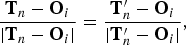(2)$$\displaystyle{{{{\bf T}_n} - {{\bf O}_i}} \over {\vert {{{\bf T}_n} - {{\bf O}_i}} \vert }}=\displaystyle{{{{{\bf T}}_n^{\prime}} - {{\bf O}_i}} \over {\vert {{\bf T}{_n^{\prime}} - {{\bf O}_i}} \vert }}\comma \; $$

where T_n and T′_n are the different transmission positions in the line under exploration, e.g. L_l, as shown in Fig. 1. Under this condition, we can further have $\vert {{{\bf T}_n} - {{\bf O}_i}} \vert - \vert {{{{\bf T}}_n^{\prime}} - {{\bf O}_i}} \vert =\vert {{{\bf T}_n} - {{{\bf T}}_n^{\prime}}} \vert $.

Obviously, for the objects in the concerned line, T_n and T′_n have the same illumination angles. But for the objects out of this line, they have different illumination angles. Therefore, for the objects in the concerned line, the same distance between T_n and T′_n would induce the same time-delay difference given by

(3)$$\eqalign{t_{{T_n}\comma {{T}_n^{\prime}}}^{diff} & = {t_{{R_m}\comma {O_i}\comma {T_n}}^{\prime}} - {t_{{R_m}\comma {O_i}\comma {{T_n^{\prime}}}}^{\prime}} \cr & = [ {\vert {{{\bf T}_n} - {{\bf O}_i}} \vert - \vert {{{{\bf T}}_n^{\prime}} - {{\bf O}_i}} \vert } ] /c = \vert {{{\bf T}_n} - {{{\bf T}}_n^{\prime}}} \vert /c.}$$

However, it would induce different time-delay differences for the objects out of this line, due to the fact that $\vert {{{\bf T}_n} - {{\bf C}_j}} \vert - \vert {{{{\bf T}}_n^{\prime}} - {{\bf C}_j}} \vert \ne \vert {{{\bf T}_n} - {{{\bf T}}_n^{\prime}}} \vert $.

According to (3), if taking the transmission position T₁ as a reference, we have

(4)$$p\lpar t - {t_{{R_m}\comma {O_i}\comma {T_n}}^{\prime}} + t_{{T_n}\comma {T_1}}^{diff} \rpar = p\lpar t - {t_{{R_m}\comma {O_i}\comma {T_1}}^{\prime}}\rpar \comma \; $$

where the time-delay difference $t_{{T_n}\comma {T_1}}^{diff} $ only depends on the transmission positions. This implies that, for the objects located in the line under exploration, their time-delays with respect to different transmission positions could be compensated and then aligned by the operation given by (4).

Based on the signal model given by (1), let us consider a “time-shift & accumulation” operation which is described as

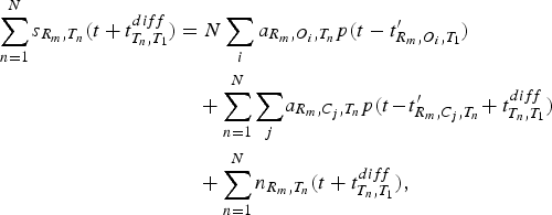(5)$$\eqalign{\sum\limits_{n = 1}^N {s_{{R_m}\comma {T_n}}}\lpar t + t_{{T_n}\comma {T_1}}^{diff} \rpar & = N\sum\limits_i {a_{{R_m}\comma {O_i}\comma {T_n}}} p\lpar t - {{t}_{{R_m}\comma {O_i}\comma {T_1}}^{\prime}}\rpar \cr & \quad + \sum\limits_{n = 1}^N \sum\limits_j \!{a_{{R_m}\comma {C_j}\comma {T_n}}} p\lpar t \!-\! {{t}_{{R_m}\comma {C_j}\comma {T_n}}^{\prime}} \!+ t_{{T_n}\comma {T_1}}^{diff} \rpar \cr & \quad + \sum\limits_{n = 1}^N {n_{{R_m}\comma {T_n}}}\lpar t + t_{{T_n}\comma {T_1}}^{diff} \rpar \comma \;} $$

where n is the index of the transmission positions. The first and second terms of the right part of the equation, are the accumulations of responses scattered from the objects located in and out of the line under exploration, respectively. The third term is noise. It is noted that

• • in the line under exploration: the responses of the objects (O _i) are time-shifted, aligned and then accumulated. It is a coherent operation, where the parameter $t_{{T_n}\comma {T_1}}^{diff} $ is used for time-delay correction. Responses are enhanced for N times as compared with the case of single transmission data.

• • Out of the line under exploration: the responses of objects (C _j) are non-uniformly time-shifted, disturbed, and then accumulated. It is an incoherent operation, because ${a_{{R_m}\comma {C_j}\comma {T_n}}} \ne {a_{{R_m}\comma {C_j}\comma {{T}_n^{\prime}}}}$, and the fact that the parameter $t_{{T_n}\comma {T_1}}^{diff} $ could further disturb the arriving-time of the responses. As a consequence, for a certain time-slot, the responses from objects located on different ellipses (or ellipsoids) are non-uniformly time-shifted and accumulated. Hence, these responses are attenuated as compared with the output of the coherent operation above.

The main steps of the operation are summarized as follows:

1. (a) move the transmitter along a certain track, e.g. L_l;

2. (b) execute the “time-shift & accumulation” operation to enhance the signal. In the operation, responses of objects located in L_l are aligned, whereas responses of objects out of L_l are non-uniformly time-shifted (disturbed);

3. (c) target detection along the track L_l;

4. (d) repeat (a)–(c) for other tracks.

IV. DATA-PROJECTION AND THE SPECTRUM-SHIFT

A) Data-projection

As shown in Fig. 3, X is an arbitrarily scatterer located on the surface of the concerned target (e.g. O _i in Fig. 1). X₀ denotes a reference point (e.g. the center of surface).

Fig. 3.

Illumination geometry with respect to the target's surface plane.

Owing to the existence of walls in the indoor environment, excess time-delay occurs when rays penetrate wall materials. Denote as ζ(B, A) the excess time delay existing in the propagating path starting from point A and ending at point B. Then, the propagation time between the transmitter T_n, scatterer X, and receiver R_i can be expressed as

(6)$$t^{\prime}\lpar {{\bf R}_i}\comma \; {\bf X}\comma \; {{\bf T}_n}\rpar = d\lpar {{\bf R}_i}\comma \; {\bf X}\comma \; {{\bf T}_n}\rpar /c + \zeta \lpar {{\bf R}_i}\comma \; {\bf X}\rpar + \zeta \lpar {\bf X}\comma \; {{\bf T}_n}\rpar \comma \; $$

where d(R_i, X, T_n) = | R_i − X| + | T_n − X| is the range of propagation.

Suppose the target locates in the far field of the radar sensors, and the spatial extent is far less than its distance to the radar sensors. It is reasonable to assume that all the scatterers on the concerned extended target have the same excess time-delay. This implies that the excess time-delay does not change with the variation of scatterer's position X. Mathematically, it can be assumed that

$$\displaystyle{{\partial} \over {{\partial} {\bf X}}}[ {\zeta \lpar {{\bf R}_i}\comma \; {\bf X}\rpar + \zeta \lpar {\bf X}\comma \; {{\bf T}_n}\rpar } ] = 0.$$

Then (6) can be expanded at the nearby of X₀ as

(7)$$t^{\prime}\lpar {{\bf R}_i}\comma \; {\bf X}\comma \; {{\bf T}_n}\rpar \approx t^{\prime}\lpar {{\bf R}_i}\comma \; {{\bf X}_0}\comma \; {{\bf T}_n}\rpar + \tau .$$

The variable τ is the time-delay induced by the variation of scatterer positions,

(8)$$\tau = { {\hbox{gra}{\hbox{d}_x}\lpar {d\lpar {{\bf R}_i}\comma \; {\bf X}\comma \; {{\bf T}_n}\rpar } \rpar } \vert _{{\bf X} = {{\bf X}_0}}} \cdot \Delta {\bf X}/c = {{\bf p}_{ref}} \cdot \Delta {\bf X}\comma \; $$

where ${{\bf p}_{ref}} = { {\hbox{gra}{\hbox{d}_x}\lpar {d\lpar {{\bf R}_i}\comma \; {\bf X}\comma \; {{\bf T}_n}\rpar } \rpar } \vert _{{\bf X} = {{\bf X}_0}}}/c$ is a reference vector selected. ΔX = X − X₀ is a vector on the target-surface plane. grad_x(·) is a gradient operator with respect to the variable X. According to the concept of gradient operation, grad_x(d(R_i, X, T_n)) points to the direction of the greatest rate of change of the distance d(R_i, X, T_n). It determines the direction of p_ref. Here, “·” is a dot-product operator. Via the dot-product operation given in (8), the vector ΔX is projected onto the direction of the reference vector p_ref.

Similarly, consider the time-delay of the signal received by R _j, whose reception angle is different from that of R _i. When projecting the data onto the same reference vector p_ref, the time-delay can be given as

(9)$$t^{\prime}\lpar {{\bf R}_j}\comma \; {\bf X}\comma \; {{\bf T}_n}\rpar \approx t^{\prime}\lpar {{\bf R}_i}\comma \; {{\bf X}_0}\comma \; {{\bf T}_n}\rpar + {\gamma _{j\comma i}}\tau\comma \; $$

where γ _j,i is a scaling factor,

(10)$$\eqalign{{\gamma _{j\comma i}} & = \displaystyle{{{{ {\hbox{gra}{\hbox{d}_x}\lpar {d\lpar {{\bf R}_j}\comma \; {\bf X}\comma \; {{\bf T}_n}\rpar } \rpar } \vert }_{{\bf X} = {{\bf X}_0}}} \cdot \Delta {\bf X}} \over {{{ {\hbox{gra}{\hbox{d}_x}\lpar {d\lpar {{\bf R}_i}\comma \; {\bf X}\comma \; {{\bf T}_n}\rpar } \rpar } \vert }_{{\bf X} = {{\bf X}_0}}} \cdot \Delta {\bf X}}} \cr & = 1 + \displaystyle{{\lpar {{\bf U}_{{R_j}\comma {X_0}}} - {{\bf U}_{{R_i}\comma {X_0}}}\rpar } \over {{{\bf V}_{bi}} \cdot \Delta {\bf X}}}.}$$

In (10), ${{\bf V}_{bi}} = {{\bf U}_{{T_n}\comma {X_0}}} + {{\bf U}_{{R_i}\comma {X_0}}}$. ${{\bf U}_{{T_n}\comma {X_0}}}$ and ${{\bf U}_{{R_i}\comma {X_0}}}$ are the unit vectors of T_n − X₀, and R_i − X₀, respectively. ${{\bf U}_{{R_j}\comma {X_0}}}$ is the unit vector of R_j − X₀. It can be proven that V_bi locates on the bisector of the angle ∡R _iX ₀T _n.

In fact, (8)–(10) define a data-projection operation, in which, ΔX, the location variations of scatterers on the target-surface plane with respect to the different receivers R _i and R _j, are projected onto the same the reference vector p_ref. In other words, the location variations ΔX on the target-surface plane are translated into time-delay variations in the direction of the reference vector p_ref. In the perspective of signal processing, it would correspond to a resampling operation, in which the resampling rate is controlled by the parameter γ _j,i.

Apparently, due to the existence of the scaling factor γ _j,i, even for the same location variation ΔX on the target-surface plane, it will induce different time-delays, τ and γ _j,iτ, with respect to different illumination geometries, e.g. “T_n → X → R_i” and “T_n → X → R_j”. Consequently, it will further impact on the spectrum in frequency domain.

B) Spectrum-shift

Recalling that ${s_{{R_i}\comma {T_n}}}\lpar t\rpar $ and ${s_{{R_j}\comma {T_n}}}\lpar t\rpar $ are the responses obtained at different receivers R _i, R _j, with respect to the same transmission position T _n. Denote as ${\tilde s_{{R_i}\comma {T_n}}}\lpar t\rpar $ and ${\tilde s_{{R_j}\comma {T_n}}}\lpar t\rpar $ the expressions of ${s_{{R_i}\comma {T_n}}}\lpar t\rpar $ and ${s_{{R_j}\comma {T_n}}}\lpar t\rpar $ after they pass through the down-converter of the system. Denote as ${\hat s_{{R_i}\comma {T_n}}}\lpar \tau \rpar $ and ${\hat s_{{R_j}\comma {T_n}}}\lpar \tau \rpar $ the expressions of ${\tilde s_{{R_i}\comma {T_n}}}\lpar t\rpar $ and ${\tilde s_{{R_j}\comma {T_n}}}\lpar t\rpar $ after they are projected onto the reference vector direction. Denote as ${\hat S_{{R_i}\comma {T_n}}}\lpar \bar \omega \rpar $ and ${\hat S_{{R_j}\comma {T_n}}}\lpar \bar \omega \rpar $ the Fourier transforms of ${\hat s_{{R_i}\comma {T_n}}}\lpar \tau \rpar $ and ${\hat s_{{R_j}\comma {T_n}}}\lpar \tau \rpar $, respectively.

According to the results given in the appendix, the relative spectrum-shift between ${\hat S_{{R_i}\comma {T_n}}}\lpar \bar \omega \rpar $ and ${\hat S_{{R_j}\comma {T_n}}}\lpar \bar \omega \rpar \rpar $ can be given by

$${\Omega _{j\comma i}} = {\omega _c}\lpar {\gamma _{j\comma i}} - 1\rpar = {\omega _c}\displaystyle{{\lpar {{\bf U}_{{R_j}\comma {X_0}}} - {{\bf U}_{{R_i}\comma {X_0}}}\rpar } \over {{{\bf V}_{bi}} \cdot \Delta {\bf X}}}.$$

Apparently, it does not contain the excess time-delay-related terms. By a further investigation of (6), (A.6), and (A.7), it can be seen that the excess time-delay only impact on the phase of (A.6). But, it does not impact on the relative spectrum-shift Ω_j,i.

As discussed in the appendix, the relative spectrum-shift Ω_j,i can be further expressed as a function of angle-difference $\lpar {\theta _{{R_j}}} - {\theta _{{R_i}}}\rpar $ as

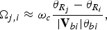$${\Omega _{j\comma i}} \approx {\omega _c}\displaystyle{{{\theta _{{R_j}}} - {\theta _{{R_i}}}} \over {\vert {{{\bf V}_{bi}}} \vert {\theta _{bi}}}}\comma \;$$

where θ _bi, ${\theta _{{R_i}}}$ and ${\theta _{{R_j}}}$ are the angles between the normal of the target surface (i.e. vector e₃ in Fig. 3) and the vector V_bi, the projections of R_i and R_j onto the plane B, respectively. Specially, we assume that the radar sensors (transmitter, receiver) and the target are located at the same plane (e.g. the sensors and the target are all located on the floor of a room). Then, if the normal of the target surface (i.e. vector e₃) also locates in the same plane (e.g. in indoor environment, a wide range of objects, such as cabinets, refrigerators, etc., are with vertical surfaces. The normals of all these vertical surfaces are located in the floor plane), the angle-difference $\lpar {\theta _{{R_j}}} - {\theta _{{R_i}}}\rpar $ given in (A.11) would be ∡R _iX ₀R _j, which is an angle-difference between the corresponding reflection directions.

In indoor environments, walls exist inevitably. It is reasonable to assume that the two sides of walls are parallel, and the rays going out the wall material can still be parallel to the incident ray (as shown in Fig. 4). Under this assumption, the angle-difference $\lpar {\theta _{{R_j}}} - {\theta _{{R_i}}}\rpar $ does not change after the wave passing through walls. That is, the wall does not change the value of $\lpar {\theta _{{R_j}}} - {\theta _{{R_i}}}\rpar $. Hence, the measured spectrum-shift Ω_j,i and the parameter γ _j,i do not change after the wave passing through walls.

Fig. 4.

The model of the wall. Assume that the rays (r ₂) going out the wall material are still parallel to the incident rays (r ₁). That is, θ ₁ = θ ₂.

In short, under the given assumptions, both the excess time-delay due to walls and the refraction effect of walls do not impact on the value of spectrum-shift Ω_j,i and also the value of the parameter γ _j,i, theoretically.

C) Signal expression after data-projection

If we neglect the influence of the phase of complex reflectivity σ, it can be inferred from (A.6) that, the spectrum-shift given in (A.7) or (A.11) is same with the shift between $\vert {{{\hat S}_{{R_i}\comma {T_n}}}\lpar \bar \omega \rpar \rpar } \vert $ and $\vert {{{\hat S}_{{R_j}\comma {T_n}}}\lpar \bar \omega \rpar \rpar } \vert $. Obviously, the operation of |·| isolates the influence of excess time-delay incurred by walls. Let ${\bar s_{{R_i}\comma {T_n}}}\lpar \tau \rpar $ and ${\bar s_{{R_j}\comma {T_n}}}\lpar \tau \rpar $ be the inverse Fourier transform of $\vert {{{\hat S}_{{R_j}\comma {T_n}}}\lpar \bar \omega \rpar \rpar } \vert $ and $\vert {{{\hat S}_{{R_j}\comma {T_n}}}\lpar \bar \omega \rpar \rpar } \vert $, respectively. The relationship between ${\bar s_{{R_i}\comma {T_n}}}\lpar \tau \rpar $ and ${\bar s_{{R_j}\comma {T_n}}}\lpar \tau \rpar $ can be given as

(11)$${\bar s_{{R_j}\comma {T_n}}}\lpar \tau \rpar \approx {\bar s_{{R_i}\comma {T_n}}}\lpar \tau \rpar \exp \lpar - j{\gamma _{j\comma i}}\tau \rpar .$$

If take the receiver R ₁ as the reference, after the data-projection operation, we have

(12)$${\bar{\bf s}_{{T_n}}} = \bar s_{{T_n}}^{ref} {\bf K}\comma \; $$

where ${\bar{\bf s}_{{T_n}}} = [ {\bar s_{{R_1}\comma {T_n}}}\comma \;{\bar s_{{R_1}\comma {T_n}}}\comma \; ...\comma \;{\bar s_{{R_M}\comma {T_n}}}{] ^T}$. The superscript T indicates the transpose operation. In addition, 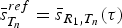$\bar s_{{T_n}}^{ref} = {\bar s_{{R_1}\comma {T_n}}}\lpar \tau \rpar $, and K = [1, exp(−jγ _2,1τ),…, exp(−jγ _M,1τ]^T.

For convenience of mathematical manipulation, if we consider the effects of unwanted contributions due to clutter c and noise n, the signal model for all transmission positions can be given as

(13)$$\eqalign{{\bf y} & = {{\bar{\bf s}}^{ref}} \otimes {\bf K} + {\bf c} + {\bf n} \cr & = {\bf x} + {\bf c} +{\bf n}\comma \; } $$

where y is a N _MN×1 vector, ${\bar{\bf s}^{ref}}=[ \bar s_{{T_1}}^{ref}\comma \; \bar s_{{T_n}}^{ref}\comma \; ...\comma \; \bar s_{{T_N}}^{ref} {] ^T}$, and ${\bf x}={\bar{\bf s}^{ref}} \otimes {\bf K}$. N _MN = M × N, where M and N are the numbers of receivers and transmission positions, respectively. The symbol ⊗ denotes Kronecker product. Noise n and clutter c are N _MN × 1 independent zero-mean complex Gaussian with known N _MN × N _MN covariance matrices M_c+n = E[(c + n)(c + n)^H]. It is noted that M_c+n is positive semidefinite and Hermitian symmetric [Reference van den Bos7]. The superscript H indicates conjugate transpose of a matrix.

According to the CLT of the probability theory [Reference Kobayashi, Mark and Turin8], if a large number of clutters from different sources (scattered from different objects) are accumulated, the statistical distribution of the sum will approach Gaussian distribution. Recalling that our scenario takes place in a cluttered indoor environment, which is with plenty of various scatterers. We assume that clutter c and noise n here could satisfy, or approach Gaussian distribution due to the “time-delay & accumulation” operations in the signal enhancement procedure. Hence, our detection problem becomes searching targets in Gaussian clutter and noise.

V. DETECTION

A) Detection problem formulation

For the detection, we define the two hypotheses:

$${H_{0\colon }}\; {\bf y} = {\bf c} + {\bf n}\; \colon \; {\rm Clutter}\; {\rm and}\; {\rm noise}\; {\rm only\comma \; }$$

$${H_{1\colon }}\; {\bf y} = {\bf x} + {\bf c} + {\bf n}\; \colon \; {\rm Target}\; {\rm plus}\; {\rm clutter}\; {\rm and}\; {\rm noise} .$$

The task is to observe the return vector y and decide which of the two hypotheses best describes the observed vector.

Suppose p(y/H ₀) and p(y/H ₁) are the conditional probability density functions of the observed vector y. The log-likelihood ratio test can be given by

(14)$$\eqalign{& \bar \Lambda \lpar {\bf y}\rpar = \ln \displaystyle{{p\lpar y/{H_1}\rpar } \over {p\lpar y/{H_0}\rpar }} \geq {{\bar k}_{th}}\comma \; \quad {H_1}\, \hbox{is}\, \hbox{true} \cr & \bar \Lambda \lpar {\bf y}\rpar = \ln \displaystyle{{p\lpar y/{H_1}\rpar } \over {p\lpar y/{H_0}\rpar }}\rpar \lt {{\bar k}_{th}}\comma \; \quad {H_0}\, \hbox{is}\, \hbox{true}\comma \; } $$

where ${\bar k_{th}}$ is the threshold. $\bar \Lambda \lpar {\bf y}\rpar $ can be further expressed as

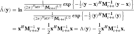(15)$$\eqalign{{\bar \Lambda ({\bf y})} &= \ln{{1 \over (2\pi )^{{N_{MN}}/2}\vert{\bf M}_{c + n} \vert^{1/2}}\exp \left\{- {1 \over 2}({\bf y} - {\bf x})^H {\bf M}_{c + n}^{ - \bf 1} ({\bf y} - {\bf x})\right\}\over{1 \over (2\pi )^{{N_{MN}}/2}\vert{\bf M}_{c + n} \vert^{1/2}}\exp \left\{- {1 \over 2}({\bf y})^H {\bf M}_{c + n}^{ - \bf 1} ({\bf y})\right\}} \cr & ={\bf x}^H {\bf M}_{c + n}^{-1} {\bf y} - {1 \over 2} {\bf x}^{H}{\bf M}_{c + n}^{ - 1} {\bf x} = \Lambda ({\bf y}) - {1 \over 2}{\bf x}^{H}{\bf M}_{c + n}^{ - 1} {\bf x},}$$

where |M_c+n| denotes the determinant of M_c+n, and M_c+n⁻¹ denotes the inverse of M_c+n. Herein, the property of Hermitian symmetric matrix is used, and let

(16)$${\Lambda \lpar {\bf y}\rpar } = {{\bf x}^H}{{\bf M}_{c + n}^{ - 1}} {\bf y}.$$

Thus, the likelihood ratio test becomes

(17)$$\eqalign{& {\Lambda \lpar {\bf y}\rpar } \geq {k_{th}}\comma \; \quad {H_1}\, \hbox{is}\, \hbox{true}\comma \; \cr & \Lambda \lpar {\bf y}\rpar \lt {k_{th}}\comma \; \quad {H_0}\, \hbox{is}\, \hbox{true}\comma \; } $$

where the threshold k _th is defined as

(18)$${k_{th}} = {\bar k_{th}} + {1 \over 2}{{\bf x}^H}{\bf M}_{c + n}^{ - 1} {\bf x}.$$

B) Detector

Based on (16), (17), a detector could be given as

$${\bf h} = {\bf M}_{c + n}^{ - 1} {\bf x} = {\bf M}_{c + n}^{ - 1} \lpar {\bar{\bf s}^{ref}} \otimes {\bf K}\rpar .$$

In fact, it is a matched filter detector, and we have Λ(y) = h^Hy. The matrix K could be set based on the values of γ _j,i or Ω_j,i given by (A.7) or (A.11).

The detector h can be further expressed as h = [h₁, h₂, ..., h_N]^T, where the element h_i ≜ [h _(i−1)·N+1, h _(i−1)·N+2,…, h _(i−1)·N+M]^T. For example, h₁ = [h ₁, h ₂,…, h _M]^T, h₂ = [h _N+1, h _N+2,…, h _N+M]^T, and so on. Similarly, we have y = [y₁, y₂,…, y_N]^T, where the element y_i is defined as y_i ≜ [y _(i−1)·N+1, y _(i−1)·N+2,…, y _(i−1)·N+M]^T. Here, the symbol i in the subscript is the index of the transmission positions.

The output of the matched filter detector can be given as

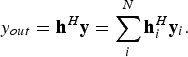(19)$${y_{out}} = {{\bf h}^H}{\bf y} = \sum\limits_i^N {\bf h}_i^H {{\bf y}_i}.$$

It gives a coherent combination of signals from N-transmission positions as shown in Fig. 1. In order to lose the requirement of the phase synchronization between different transmissions, we can incoherently combine the data from different transmissions, by

(20)$${y_{out}} = \sum\limits_i^N \vert {{\bf h}_i^H {{\bf y}_i}} \vert .$$

In fact, h_i^Hy_i in both (19) and (20) can be regarded the detection result obtained at a certain individual transmission position T _i. Then, the final output of the detector could be a coherent combination of the individual detection result h_i^Hy_i as given in (19), or an incoherent combination of all the individual detection results as given in (20).

C) Threshold and performance

The probability of detection in (19), and false alarm can be given as

(21)$${P_d} = 1 - \Phi \lpar {{{k_{th}} - {{\bf h}^H}{\bf x}} \over D}\rpar \comma \; $$

(22)$${P_f} = 1 - \Phi \left({{{{k_{th}}} \over D}} \right)\comma \; $$

where 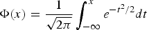$\Phi \lpar x\rpar = {1 \over {\sqrt {2\pi } }}\int_{ - \infty }^x {e^{ - {t^2}/2}}dt$, and the parameter D is defined as

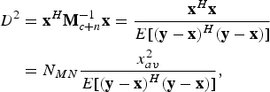(23)$$\eqalign{{D^2} & = {{\bf x}^H}{\bf M}_{c + n}^{ - 1} {\bf x} = {{{{\bf x}^H}{\bf x}} \over {E[ {{{\lpar {\bf y} - {\bf x}\rpar }^H}\lpar {\bf y} - {\bf x}\rpar } ] }} \cr & = {N_{MN}} {{x_{av}^2 } \over {E[ {{{\lpar {\bf y} - {\bf x}\rpar }^H}\lpar {\bf y} - {\bf x}\rpar } ] }}\comma} \; $$

where x Reference Moura and Jin²_av is the average signal power of x. Generally,

$${{x_{av}^2 } \over {E[ {{{\lpar y - x\rpar }^H}\lpar y - x\rpar } ] }}$$

can be regarded as the SINR at the output of the detector [Reference Poor9].

In terms of Neyman–Pearson criterion, the threshold k _th could be set as

$${k_{th}} = D\Phi \lpar 1 - {P_f}\rpar .$$

Correspondingly, the detection probability can be further given as P _d = 1 − Φ(Φ⁻¹(1 − P _f) − D).

VI. MEASUREMENT RESULTS

The measurement environment is shown in Fig. 5(a). A UWB M-sequence pseudo-noise radar developed by Ilmenau University of Technology in cooperation with MEODAT company [Reference Zetik, Sachs and Thoma10] is used in the measurement. The sensor setup is given by Fig. 5(b). The transmitter moves along track L_l, and illuminating the surroundings meanwhile. It is mounted on a program-controlled positioning unit (as shown in Fig. 5(a), the column-like object, which is attached on a rail mounted at the ceiling of the room). The positioning unit allows precise positioning of the transmitter antenna with 0.75 mm precision in two directions. The target is a concrete brick-like object with a square planar-surface (50 cm × 50 cm) as shown in Fig. 5. It is located at x = 24 cm in the track L_l, with an orientation angle 60°. R ₁–R ₄ are four receivers, receiving the scattered signals from the surroundings. They are located at different directions with respect to the target. The transmitter–target–receiver angles are 13.9°, 20.3°, 26.3°, and 31.7°, respectively. The antennas of the transmitter and receivers are omnidirectional and horn antennas, respectively. As shown in Fig. 5(b), R ₁ and R ₂ are located in the same room with the target and the transmitter, whereas R ₃ and R ₄ are located behind a 20-cm-thick concrete wall. Figure 6 shows the signals received by R ₁–R ₄. Apparently, excess time-delays exist in the signals received by R ₃ and R ₄. However, there is no excess time-delay for the signal received by R ₁ and R ₂.

Fig. 5.

Measurement setup. (a) measurement environment. The target is a concrete brick-like object with a diffuse surface. The receivers placed behind the wall are not shown in the picture. (b) Sensor setup. The target is located at x = 24 cm on the line L _l, with an orientation angle θ = 60°.

Fig. 6.

Measured signals in a realistic environment given by Fig. 5(a). The red vertical line: the theoretical position of the direct-path; the first blue peak: direct-path. The vertical axis: normalized amplitude.

In a realistic indoor environment, the response of the target is mixed with clutter and noise at the receivers. Typically, the clutter comes from objects in 3D space, such as walls, furniture, the ceiling, and also the ground, etc. Owing to the complexity of indoor environment, in a high probability, clutter is not weaker than the response of the target. In order to get a reliable detection, our first step is to enhance the responses in the line under exploration via a “time-shift & accumulation” scheme, in which the signals recorded at different transmission positions are time-shifted, aligned, and accumulated according to (5). After “time-shift & accumulation” operation, the data are projected onto the reference vector direction. This is realized by a resampling operation. Figure 7 shows the spectrum-shifts after data-projection. In the figure, ${f_{{R_1}}}{\rm \sim }{f_{{R_4}}}$ are the frequencies at which the spectra have the maximum values. Theoretically, if the target presents in the scenario, for the data acquired at the true target position and orientation, the differences between ${f_{{R_i}}}$ and ${f_{{R_j}}}$ (${f_{{R_i}}}\comma \;{f_{{R_j}}} \in [ {f_{{R_1}}}\comma \;{f_{{R_2}}}\comma \;{f_{{R_3}}}\comma \;{f_{{R_4}}}] $) should satisfy (A.7) or (A.11). Furthermore,

Fig. 7.

Measured spectrum-shifts. (a) Spectrum-shift in a “true target position, true target orientation” condition. (b) Spectrum-shifts in a “false target position, true target orientation” condition. (c) Spectrum-shifts in a “true target position, false target orientation” condition.

(24)$${{{f_{{R_i}}} - {f_{{R_1}}}} \over {{f_{{R_j}}} - {f_{{R_1}}}}} = {{{\gamma _{i\comma 1}} - 1} \over {{\gamma _{j\comma 1}} - 1}}$$

should also be satisfied.

Figure 7(a) shows the measured result obtained at the true target position and orientation. It is shown that the results approach

$${{{f_{{R_i}}} - {f_{{R_1}}}} \over {{f_{{R_j}}} - {f_{{R_1}}}}} \approx {{{\gamma _{i\comma 1}} - 1} \over {{\gamma _{j\comma 1}} - 1}}.$$

However, Figs 7(b) and 7(c) are obtained under the condition of “false position, true orientation” and “true position, false orientation”, respectively. Their results can rarely satisfy (24). As compared with (A.7) and (A.11), (24) does not demand the absolute value of ω _c, so that it is more convenient to be utilized in practice.

In Fig. 8, it shows the output of the detector when the transmitter locates at x = 200 cm, searching for the target position and orientation area.

In order to further fuse the detection results obtained at different transmission positions, the final detection could be a coherent/incoherent combination of these results according to (19) or (20). Figure 9(a) shows the estimates of the target position at different transmission positions. Figure 9(b) shows the estimated orientations. In the figures, the results for different data accumulation ranges, $c \cdot t_{{T_n}\comma {{T \prime}_n}}^{diff} $, are provided. Accumulation 1 and 2 in the figures correspond to $c \cdot t_{{T_n}\comma {{T_n^ \prime}}}^{diff}$ = 10 cm and 20 cm, respectively. It is seen that their values are distributed around the true values. As indicated by the horizontal lines, the final outputs of the coherent detector are (25 cm, 61.7°) are (24.2 cm, 60.8°) for “Accumulation 1” and “Accumulation 2”, respectively. The final outputs of the incoherent detector are (26 cm, 61.9°) and (25.2 cm, 61.0°) for “Accumulation 1” and “Accumulation 2”, respectively. It is shown that the results for “Accumulation 2” are better than “Accumulation 1” under given conditions. The results when without the data enhancement procedure is not shown in the figures, because there would be no effective results in this case.