


Projectile points are important for many reasons. Types mark intervals of past time, register activity by their gross form and use wear, and may distinguish social or cultural groups. For these and other markers of human behavior, points long have been popular subjects of study.
Some tools were handheld in use, but points usually were components of larger, composite tools. Most archaeologists regard points as integral wholes, but even the smallest hafted point is made up of parts. To its users, the different segments or “modules” of a point served different purposes and were treated differently. From the perspective of hunters, minimally, tip modules initiated wounds in animal prey, blade modules deepened them, and stems articulated the exposed blade to the composite tool. Modularity may be resolved even more finely: stem modules are defined by overall size and shape, whereas fluted points have more specific functions related to adhesion to mastics in the haft. Understanding how blade and stems, or their own parts, worked as modules and together to propel a point or provide mass to aid thrust was probably critical to hunting success.
People likely perceived point modules in accordance with their function. For example, by their acuity, length, and plan form, edges could comprise modules (e.g., during beveling) or perhaps components of larger modules of the tip (if edge properties assisted penetration) or of the blade (if they aided wound expansion). If points also functioned as knives or other tools, different modules may have had joint or dual purposes (for example, blades deepen wounds, while their edges also are useful in filleting or scraping) that forced compromises in their design. Point segments may have comprised modules of a particular size and configuration for some purposes like use as weapon tips, as well as modules of different sizes and configurations for other purposes. Depending on the analytical purpose, points can be treated as wholes or as things of sometimes complexly organized parts.
Obviously, points cannot grow, but they can shrink because damage or dulling necessitates repair by resharpening. Therefore, points can change in size and shape during their use lives, a quality that recommends modular approaches to their study because some modules may change more and some less in the process and proportions between them may change greatly. Changeability as an integral property of points may seem paradoxical, but specimens may experience varying degrees and patterns of reduction in use that any comprehensive treatment of their variation must consider.
Traditionally, archaeology treated points mostly as wholes, often simply by classifying them as Type X or Y based on their overall form (e.g., Justice Reference Justice2002). Even advanced studies usually treat points as wholes, not only in analysis of the attributes that all modules share (e.g., tool stone) or those that measure their collective magnitude (e.g., mass) but also in measurement. Usually, we define and measure whole-object dimensions (e.g., length) that crosscut modules and whose variation among specimens or over any point's use life may differ between modules. Of course, dimensions may be measured separately for any modules defined. But measuring the length or width of points treats them as undifferentiated wholes and obscures the segmentation—modularity—that may inhere in them.
To illuminate the problem of parts and wholes, this study considers a holistic approach to point morphology. We use three-dimensional (3D) models of points from a controlled experiment and their 3D morphometrics to assess the effects of resharpening on the variation and covariation between point wholes and their parts as modules. Our broader contribution to lithic analyses is to suggest that signals of modularity coupled with allometry may indicate that curation could have played a role in generating such patterning.
Morphometric Analysis of Points
The application of landmark-based geometric morphometrics (LGM) to point analysis has quietly revolutionized the field (Shott Reference Shott2014). LGM characterizes whole-object form much more comprehensively than do traditionally reported dimensions, and associated software permits more thorough analysis of point size and shape than is possible otherwise. But detail in characterization is only one of LGM's virtues. From its origins in biology, LGM has acquired a set of concepts and associated analytical methods that facilitate a modular view equally relevant to points and to organisms.
LGM originated to characterize the size and shape not only of whole organisms but also of their anatomical modules (e.g., limbs, organs) and their geometric configurations. During individuals’ growth or over evolutionary time, modules’ size and shape can vary, and they can covary with one another in strong or weak degrees. The strength of covariation between modules describes their degree of integration.
In LGM studies, modules are sets of contiguous landmarks (2D or 3D coordinates of locations on larger wholes) whose covariation is greater within the module than they are with landmarks outside the module. Thus, they are “tightly integrated internally but relatively independent from other . . . modules” (Klingenberg Reference Klingenberg2008:116). Modules thus are entities, components of large wholes. Integration is the degree of covariation among the modules that comprise the whole: the “coordinated movement of the [modules] of the structure relative to one another” (Klingenberg Reference Klingenberg2008:117). Of course, some covariation integrates all parts of larger wholes; sets of objects do not vary by kaleidoscopic randomness. Modularity measures the degree to which covariation patterns geometrically within the whole, integration the degree to which separate modules covary strongly or weakly. Modules of any size, shape, and location may be defined for any analytical purpose. Defining modules is a statement of hypothesis that requires testing in the variation found among study specimens.
For various reasons, what applies to organisms’ modules like limbs and organs applies equally to points: whole objects are divisible into modules. Modularity and integration can be studied at levels from individual growth to evolutionary change—developmental/ontogenetic to evolutionary, respectively, in Klingenberg's (Reference Klingenberg2008:117–119) terms. Our study concerns allometric variation in points, which is analogous to ontogenetic allometry in biology. Allometry—the change in shape with a change in size—may characterize variation not only between point types but also among specimens within types, as a function of the reduction for maintenance that points may experience from first to last use. Because “types of modularity and integration closely parallel . . . types of allometry” (Klingenberg Reference Klingenberg2008:120), they engage allometric variation and its analysis.
Allometry and Reduction
During use, curated stone tools were damaged or dulled and then resharpened. Unless all tool modules were resharpened in proportion to their sizes, some must have experienced disproportionate resharpening and therefore reduction. Archaeologists sometimes refer to this disproportion as the “Frison effect” (Frison Reference Frison1968). It also is allometry: a change in proportions among modules (and therefore shape) with a change in size. Hoffman (Reference Hoffman and Carr1985) extended this effect to the study of points, arguing that reduction concentrated changes on blade modules more than on stems.
If modularity occurs, then different modules require separate treatment for some analytical purposes. Research can test modularity by comparing the covariation of traits within modules to their covariation with traits in other segments. Most studies to date document allometric reduction effects, usually in 2D models of archaeological specimens. Investigations of modularity are uncommon (but see González-José and Charlin Reference González-José and Charlin2012). The reduction thesis argues that both allometry's cause—damage repair by resharpening—and its effects on size and shape characterize the life history of tools (Iovita Reference Iovita, Lycett and Chauhan2010; Shott Reference Shott, Clarkson and Lamb2005). However, not all stone tools were necessarily resharpened throughout their life history; reduction allometry was probably common but not universal.
Archaeologists have documented allometry from many times and places in many tool types, including unifacial scrapers and flake tools (e.g., Ahler and Geib Reference Ahler and Geib2000; Blades Reference Blades2003; Dibble Reference Dibble1987; Goldstein Reference Goldstein2014; Hiscock and Attenbrow Reference Hiscock and Attenbrow2005; Iovita Reference Iovita, Lycett and Chauhan2010, Reference Iovita2011; Morales Reference Morales2016; Sahnouni et al. Reference Sahnouni, Schick and Toth1997; Shott and Weedman Reference Shott and Weedman2007). The reduction thesis is particularly well documented in bifaces (e.g., Andrefsky Reference Andrefsky1997, Reference Andrefsky2006; de Azevedo et al. Reference de Azevedo, Charlin and González-José2014; Bement Reference Bement, Clark and Collins2002:136; Buchanan Reference Buchanan2006; Charlin and Cardillo Reference Charlin, Cardillo, Buchanan, Eren and O'Brien2018; Charlin and González-José Reference Charlin and Rolando González-José2018; Ellis Reference Ellis2004; Flegenheimer and Weitzel Reference Flegenheimer and Weitzel2017:150; González-José and Charlin Reference González-José and Charlin2012; Hashizume Reference Hashizume, Larson, Kornfeld and Frison2009; Iovita Reference Iovita2011; Iovita and McPherron Reference Iovita and McPherron2011; Iriarte Reference Iriarte, Consens, Mazz and Curbelo1995; Lerner Reference Lerner and Shott2015; Li et al. Reference Li, Kuman and Li2015; Loyola et al Reference Loyola, Núñez, Aschero and Cartajena2017:21–22, Figure 14; Miller Reference Miller2018:93–99; Peterson Reference Peterson1978:141, Fig. 2; Prentiss et al. Reference Prentiss, Walsh, Skelton, Markes and M.Straffen2016; Serwatka Reference Serwatka2015; Shott and Ballenger Reference Shott and Ballenger2007; Shott et al. Reference Shott, Hunzicker and Patten2007; Skinner Reference Skinner2018; Smallwood et al. Reference Smallwood, Jennings and Pevny2018; Suárez Reference Suárez2011:179–183, Reference Suárez, Robinson and Sellet2017; Wheat Reference Wheat, Raymond, Loveseth, Arnold and Reardon1975; Wilmsen and Roberts Reference Wilmsen and Roberts1978:108–120), even in relatively crude Middle Paleolithic bifaces (e.g., Presnyakova et al. Reference Presnyakova, Braun, Conard, Feibel, Harris, Pop, Schlager and Archer2018:Table S4). Reduction is also reported in ethnographic sources, mostly in flake tools and unifaces, because bifaces are rare in such accounts (e.g., Hayden Reference Hayden and Wright1977; Sahle and Negash Reference Sahle and Negash2016; Shott and Sillitoe Reference Shott and Sillitoe2005; Tindale Reference Tindale1965; Weedman Reference Weedman2000).
Buchanan's (Reference Buchanan2006) analysis of archaeological Folsom points from the North American plains is particularly relevant to our study. He defined a set of “inter-landmark distances” (ILDs) between locations that included the tip, base corners, and midpoint and points of maximum width (Buchanan Reference Buchanan2006:Figure 2, Table 3). This scheme provided a different, somewhat more detailed 2D description of point form than standard dimensions. Buchanan measured point size as 2D plan area size and regressed the log-transformed ILDs individually on log-area. He found allometric variation with size in several ILDs (Buchanan Reference Buchanan2006:195, Table 6) indicated. Corroborating Buchanan, others reported similar results for linear dimensions, along with mass and allometric measures (Miller Reference Miller2018:90–93; Shott Reference Shott2020; Shott et al. Reference Shott, Hunzicker and Patten2007:212, Table 5): length and all ratios were positively allometric, whereas width and thickness were negatively allometric. Buchanan's approach represented an advance, suggesting that many ILDs likely vary with the degree of reduction that points experienced. However, it is essential not to treat some dimensions (e.g., “BW,” width at one-third of total length above base corners) as design attributes. The location of these dimensions changes with reduction because the total length from which they are calculated declines with reduction.
The reduction thesis and the allometry and modularity it engenders have important implications. One is typological. Changes in specimens of a single original type's size and shape resulting from resharpening can cause them to be confused with different types of points (e.g., Hoffman Reference Hoffman and Carr1985) and flake tools (e.g., Dibble Reference Dibble1987; Hiscock and Attenbrow Reference Hiscock and Attenbrow2005). Understanding allometry's effects on points requires distinguishing at least blade and stem modules. Stems may change in use less than blades, both because blades usually are bigger ceteris paribus and they can experience more damage than stems, thereby requiring more resharpening (Flegenheimer and Weitzel Reference Flegenheimer and Weitzel2017:150; Loendorf et al. Reference Loendorf, Rogers, Oliver, Huttick, Denoyer and Kyle Woodson2019:358; Odell and Cowan Reference Odell and Cowan1986:204). Resharpening decreases blade length substantially; blade (less likely stem) width may decline, but thickness changes little, if at all (e.g., Andrefsky Reference Andrefsky1997; Ellis Reference Ellis2004; Hashizume Reference Hashizume, Larson, Kornfeld and Frison2009:279; Hoffman Reference Hoffman and Carr1985; Peterson Reference Peterson1978; Shott and Ballenger Reference Shott and Ballenger2007; Shott et al. Reference Shott, Hunzicker and Patten2007:Table 1). Depending on the degree and pattern of reduction, those changes can produce sufficient variation in size and form at discard to make specimens of the same original type appear to be different types (Hoffman Reference Hoffman and Carr1985). For instance, “San Jon” points may be merely a reduced version of Firstview points (Wheat Reference Wheat, Raymond, Loveseth, Arnold and Reardon1975). Reduction also can make specimens in different types look similar. Among Patagonian stemmed-point types, “reduction constraints impose some limitations in phenotypic variability, leading to shape convergence among different types of . . . points” (Charlin and Cardillo Reference Charlin, Cardillo, Buchanan, Eren and O'Brien2018:123). Valid typological judgments of stone tools must take reduction effects into account.
The reduction thesis has implications beyond typology, certainly for points. Reduction patterns suggest kinds of use by identifying the edges or segments of tools that were retouched. In addition, the degree of reduction is a measure of curation, an important theoretical concept (Binford Reference Binford and Renfrew1973; Shott Reference Shott1996). Tools vary in their curation rates. Just as plotting the distribution of metric dimensions like length or width is informative for some purposes, plotting the distribution of reduction measures among specimens indicates assemblage accumulation rates and type composition (Dibble Reference Dibble1987; Surovell Reference Surovell2009). Reduction distributions calibrate discard rates of tool types to common scales and implicate causes of discard (Shott Reference Shott, Iovita and Sano2016). Fitted to the Weibull model, for instance, distributions indicating a constant discard rate, regardless of the degree of curation, identify chance as a cause of discard, whereas those indicating that the discard rate increases with curation implicate attrition. Moreover, different ranges of the Weibull shape parameter β implicate different failure scenarios. When 1 < β < 2, failure rate increases at a decreasing rate consistent with early wear-out failure, when β = 2 failure increases at a constant rate, and when β >2 failure increases at increasing rate (e.g., Douglass et al. Reference Douglass, Lin, Braun and Plummer2018; Morales Reference Morales2016; Shott and Seeman Reference Shott and Seeman2017:732). Similarly, reduction distributions can distinguish between, for instance, competing scenarios of Folsom hunting practices by linking the duration of point use—and, by extension, distributions themselves—to different assumptions about group size and hunting rates (Hunzicker Reference Hunzicker2005:55–60). Reduction patterns within or between tool types comprise an integral characteristic of type specimens just like their metric dimensions (Iovita Reference Iovita, Lycett and Chauhan2010:236).
Beck's (Reference Beck1995:234–237) selectionist study revealed that longevity and the related quality of impact resistance and, by extension, curation rate distinguished Great Basin dart types. Side-notched points were selected against partly due to their lower impact resistance and resulting shorter use lives. Degrees of curation and the form of their reduction distributions can test theoretical models of tool use and wider adaptive practices. Miller (Reference Miller2018:55–63) used the marginal-value theorem to model points as resource patches, relating their degree of utility extracted—therefore reduction—to varying hunting-return rates. This treatment makes reduction a behavioral variable to be explained by, and thereby tracking, long-term adaptive processes leading in Miller's study to the origins of agriculture. In the process, the argument both invokes the utility concept (Shott Reference Shott1996) and makes the form of point types’ reduction distributions (Miller Reference Miller2018:Figure 3.1) relevant to sophisticated behavioral modeling. The use of multiple reduction measures and their multifactorial reconciliation establish comparability between measures and studies (Shott and Seeman Reference Shott and Seeman2017), quantifying the degree of curation and grounding behavioral models in data.
On balance, “reduction is an important source of variation on size and shape differentiation between point assemblages” (Charlin and González-José Reference Charlin and Rolando González-José2018:169). Because reduction is not necessarily proportional, “major distinctions between groups of points, when measured using blade characteristics, are likely the result of differential resharpening activities” (Prentiss et al. Reference Prentiss, Walsh, Skelton, Markes and M.Straffen2016:127). Precisely because of such differential patterns, analysis should avoid freely combining characters from blades and stems that might comprise separate modules. The work of Prentiss and colleagues (Reference Prentiss, Walsh, Skelton, Markes and M.Straffen2016:124, Figures 10–12), for instance, yielded phylogenetic inferences from separate analyses of point stems and blades that were obscured by treatment that combined those modules.
Some researchers, however, disagree on the effects of resharpening. Although Buchanan (Reference Buchanan2006) found considerable evidence for allometry in Folsom-point variation using 2D outline methods applied to a sample of midcontinental Clovis points, Buchanan and Collard (Reference Buchanan and Collard2010; see also Buchanan et al. Reference Buchanan, David Kilby and Huckell2015) argued that Clovis points either experienced little resharpening reduction in use or little allometric shape change. In their view, any resharpening that occurred was proportional among all dimensions and modules, with only a possible reduction in size that did not involve significant shape change. Inferring that Folsom points at Lindenmeier regularly were resharpened, mostly on blades, and that the resulting reduction altered points’ forms disproportionately (i.e., a reduction thesis stated decades before the question acquired salience), Wilmsen and Roberts concluded that it “must be tested before its validity can be ascertained” (Reference Wilmsen and Roberts1978:111). Following from Buchanan (Reference Buchanan2006), our study is designed to test Wilmsen and Roberts's view and the broader reduction thesis, in part in an attempt to resolve uncertainties. In addition to archaeological specimens, our study includes experimental specimens that provide independent control over resharpening and other effects that can resolve the question.
Approaches to Point Reduction
As mentioned, point reduction is observed in many contexts. There is no reason to doubt that Folsom points might be subject to reduction allometry. In fact, damage and repair are central to models of Folsom design and use (Ahler and Geib Reference Ahler and Geib2000; Hofman Reference Hofman, Stanford and Day1992:212–213), and empirical evidence of resharpening is common (Bement Reference Bement and Amick1999:113; Titmus and Woods Reference Titmus, Woods, Bonnichsen and Turnmire1991:127; Wilmsen and Roberts Reference Wilmsen and Roberts1978:108–111). Previous studies of point reduction used geometric or allometric measures. Geometric ones included retouch invasiveness (Andrefsky Reference Andrefsky2006), plots of blade edge-angle against length (Hoffman Reference Hoffman and Carr1985:581–583), and sharpness indexes approximating the geometry of point form by a set of detailed measurements near the specimen tips (Lerner Reference Lerner and Shott2015; Quinn et al. Reference Quinn, Andrefsky, Kuijt, Finlayson and Andrefsky2008). Allometric measures included simple ratios of length-to-thickness (L/T) and mass-to-thickness (M/T; Iriarte Reference Iriarte, Consens, Mazz and Curbelo1995:143–144, Figure 3) validated in earlier analysis of the current dataset (Shott et al. Reference Shott, Hunzicker and Patten2007) and the ratio of shoulder angle to blade length (Suárez Reference Suárez2011:182). Reduction allometry also is documented using Fourier methods (Iovita Reference Iovita, Lycett and Chauhan2010, Reference Iovita2011).
Particularly valuable, however, are studies that use LGM methods (e.g., de Azevedo et al Reference de Azevedo, Charlin and González-José2014; González-José and Charlin Reference González-José and Charlin2012), because compared to traditional analytical approaches, LGM methods at once are richer and more detailed in data capture and more amenable to analysis using more powerful methods. That is, they approximate the fullness of 2D and especially 3D form better than do orthogonal dimensions or ILDs. (Most studies cited earlier analyzed 2D outlines or other characterizations of points.) LGM also can define modules, which is not easily accomplished in ILD studies. As a result, LGM analysis can test explicitly for modular integrity and allometry. (MacLeod's [Reference MacLeod2019] pixel-based method also deserves consideration in future research.) Biological analysis often uses LGM to study modularity and allometry characterizing not only physical growth and development but also possibly phylogenetic relationships between taxa (e.g., Adams and Otárola-Castillo Reference Adams and Otárola-Castillo2013).
Yet few of the stone-tool reduction measures noted earlier have been tested and validated in experimental data, and even fewer use LGM methods. Whatever ambiguities may inhere in the interpretation of LGM analysis of archaeological specimens are controlled for in experimental studies that furnish independent evidence for the causes invoked, such as allometry. Goodyear's (Reference Goodyear1974:Figure 12) classic example of the progressive reduction of a single Dalton-point replica documented the changing proportion among orthogonal dimensions. He made, used, and resharpened the point over four cycles, from original size and shape to unworkable remnant (Goodyear Reference Goodyear1974:28). Resharpening occurred on the blade only, the stem experiencing no reduction. Essentially, this made Goodyear's experiment a null case of reduction confined strictly to the blade (Shott Reference Shott2020:Figure 2a). The experiment suggested a disproportionate reduction in width on the blade, not stem, and at varying rates, with more width reduction occurring in the first than in successive resharpenings, compared to length; of course, there was patterned variation in the ratios of both blade area to stem area and blade length to stem length, because only the former changed during the experiment. Trivially, the Dalton replica was reduced by resharpening. Nontrivially, that reduction was attended by systematic variation in ratios between dimensions and in the relative size of the blade and stem modules. Skinner (Reference Skinner2018:37–49) documented similar effects in Western Stemmed Tradition experimental replicas. Analytical approaches that fail to distinguish stem and blade modules risk obscuring informative variation in resharpened points.
Materials and Methods
We report analysis of reduction effects in experimental replicas of Paleoindian Folsom points (Hunzicker Reference Hunzicker2005, Reference Hunzicker2008). Earlier analysis of this dataset used dimensions and other measures of specimen size (length, area, mass [of chert originals as reported by Hunzicker, not resin casts]) and simple ratios computed by dividing each of them by near-constant thickness (Shott et al. Reference Shott, Hunzicker and Patten2007) or ILDs (Shott Reference Shott2020). In our study, LGM methods test for the effects of allometry and modularity. In Klingenberg's (Reference Klingenberg2008) terms, our focus is on developmental or ontogentic modularity and the resulting allometry. In contrast to most previous studies that analyzed 2D point models, ours involves 3D models.
Data
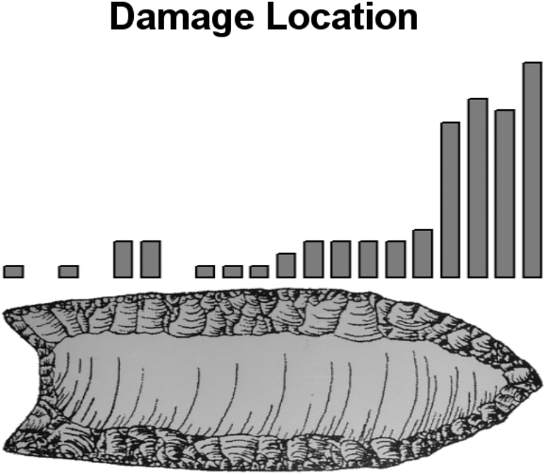
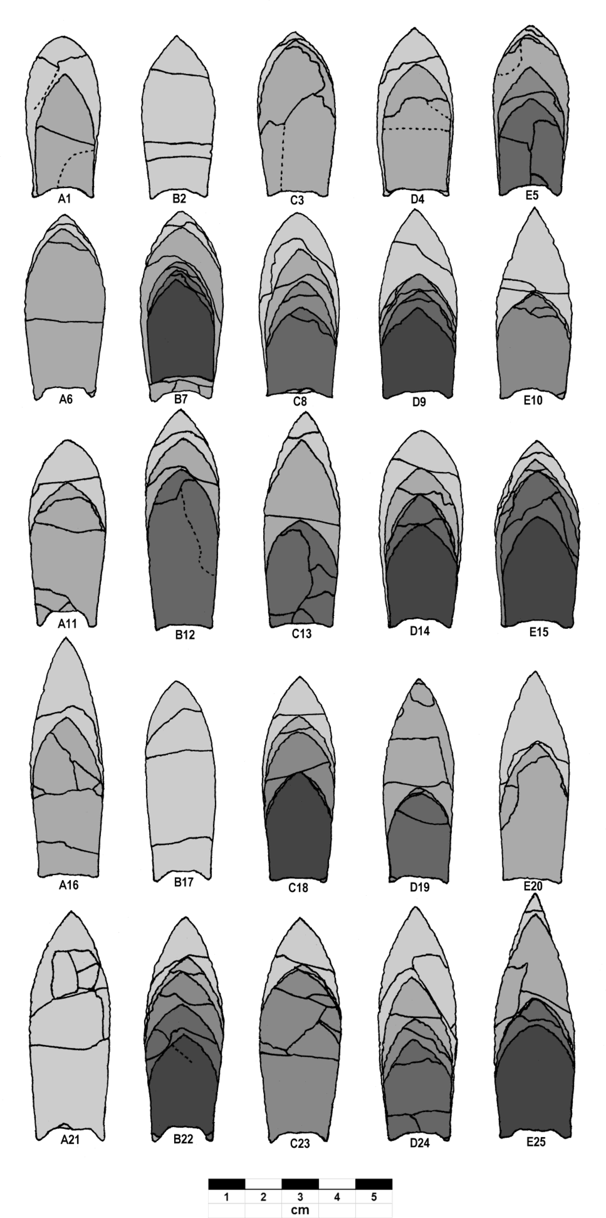
Hunzicker studied 25 Folsom points made by Bob Patten, an accomplished knapper (Patten Reference Patten2005). Using several hafting and propulsion methods, Hunzicker fired spears tipped with the points into the rib cages of slaughtered cows. The experiment's chief goal was to gauge the durability and performance of combinations of hafting and propulsion (Hunzicker Reference Hunzicker2005:32–47). After each cycle of use and damage, points were removed from hafts and examined for type and the pattern and extent of damage. Except when damage was catastrophic, with the point shattering into too many pieces to salvage, Patten repaired the points by careful resharpening in “a complex process involving simultaneous efforts to restore symmetry, reduce tip thickness, [and] improve alignment” (Hunzicker Reference Hunzicker2005:28). Most resharpening occurred, as Wilmsen and Roberts (Reference Wilmsen and Roberts1978:108–111) expected, on the exposed blade and tip (see also Ahler and Geib Reference Ahler and Geib2000; Flegenheimer and Weitzel Reference Flegenheimer and Weitzel2017; Odell and Cowan Reference Odell and Cowan1986). Figure 1 illustrates this pattern of damage location. Yet stems wrapped in sinew and covered with mastic also could and did suffer damage in use. Even when stems were not damaged, repair and resharpening of the blades, when they were removed from the hafts, could impinge on stems and thereby reduce them (Hunzicker Reference Hunzicker2005:27–29). That is, reduction by resharpening occurred mostly on blades but somewhat on stems as well. The effect was to shorten the points (and, of course, reduce their mass) but to alter other dimensions little if at all, thereby changing the shape and the proportions among dimensions (Figure 2). Allometry that may attend this process resides mostly, not entirely, on blades.
Major patterns of damage location in Hunzicker Folsom replicas, showing concentration on tip and blade (from Hunzicker Reference Hunzicker2005:Figure 7).
Hunzicker Folsom replicas showing pattern and range of reduction by breakage and repair. Progessively reduced versions of each original specimen shown in darker shading. Dashed lines indicate visible fractures that did not detach (from Hunzicker Reference Hunzicker2008:Figure 6).
Most experimental points survived the first cycle of damage and repair, and 22 of 25 experienced two or more cycles. Hunzicker made resin casts of specimens before their first use and after each repair cycle, yielding a total of 82 versions of the 25 originals. Overall, points survived an average of about 3.3 cycles (82 cycles for 25 points). Therefore, we know how long each replica was used and how much it was reduced in each of as many as five cycles encompassing first use and subsequent repair and reuse. For most original specimens and their repaired and reduced versions, successive use-and-repair intervals were numbered successively 1, 3, 5, 7, and 9, limited, of course, by the number of cycles that each survived. For instance, specimen B22 experienced four cycles of repair after first use. Accordingly, its first use was as B22.1, then progressed through B22.3, B22.5, and B22.7 before culminating in B22.9. (Intervening even numbers usually were reserved for damaged but not yet repaired versions of each specimen in each repair interval. Although Hunzicker also made casts of these damaged versions, they are not considered in this study.)
Mean length ranged from 60.0 mm before first use to 31.4 mm by final reuse stage, with mean maximum width ranging from 22.5 to 20.7 mm and mean thickness from 4.8 to 4.5 mm over the same range of uses (Shott et al. Reference Shott, Hunzicker and Patten2007:Table 1). This range of values resembles mean dimensions of finished and used Folsom points reported by Lassen (Reference Lassen2016:Tables S1–4) across the Plains, Ahler and colleagues (Reference Ahler, Frison, McGonigal, Clark and Collins2002:Table 5.7) for the northern Plains, Asher (Reference Asher2015:Table 11) for the central Plains, and Collins (Reference Collins and Amick1999:26) and LeTorneau and Baker (Reference LeTorneau, Baker, Clark and Collins2002:Table 3.4) for the southern Plains. At the type site, the sole intact Folsom specimen (AMNH 20.2.5865) measured 56 mm in length, 24.2 mm in maximum width, and 3.9 mm in maximum thickness, and two intact specimens described as “reworked” (Sn23/CAVO-116 and Sn24/B.Burchard; Meltzer Reference Meltzer2006:Table 8.2) measured between 32 and 35 mm in length, 19 and 22 in maximum width, and 4.0 and 4.6 in maximum thickness (Meltzer Reference Meltzer2006:Table 8.4). At Lindenmeier, weighted means were 35.7 mm for length, 18.6 mm for maximum width, and 3.8 mm for maximum thickness, although these measurements referred to “whole points (including fragments)” (Wilmsen and Roberts Reference Wilmsen and Roberts1978:Table 43; see also Ahler and Geib Reference Ahler and Geib2000:808), so may not be strictly comparable to those cited earlier. Ahler and Geib (Reference Ahler and Geib2000:813; see also Collins Reference Collins and Amick1999:26) considered the maximum length of unused Folsom points to be approximately 75 mm and the length of depleted specimens to be roughly half that (although according to Collins, resharpened Folsom points “as short as ca. 25 mm are not uncommon” [Reference Collins and Amick1999:26]). Hunzicker (Reference Hunzicker2005:44) considered 30 mm a minimum value for the length of Folsom points. Consistent with these expectations, mean dimensions in the highly reduced Cooper assemblage are 33.7 mm for length, 19.3 mm for maximum width, and 3.5 mm for maximum thickness (Bement Reference Bement and Amick1999:Table 1). In contrast, Lassen's (Reference Lassen2016) dataset ranges widely in length from less than 20 mm to 75 mm, although specimens more than 50 mm in length form a relatively small right tail.
On balance, Folsom replicas seem reasonably faithful in major orthogonal dimensions to archaeological specimens documented over a wide geographic range. Yet judging by these studies, they may be somewhat shorter at first use and slightly thicker on average than archaeological specimens, even though their thickness falls squarely in the range reported by Asher (Reference Asher2015:Table 11). Assuming these differences, their effects on point longevity and pattern and degree of reduction are unknown.
Here and elsewhere (e.g., González-José and Charlin Reference González-José and Charlin2012), the tip angle formed by the converging blade margins is considered an original design attribute but one also subject to change as reduction progresses. For instance, Ahler and Geib observed a pattern “in which the longest whole points or most lengthy distal tip fragments . . . have the most acute front [tip] angles” (Reference Ahler and Geib2000:809). Consistent with this observation, tip angles of Folsom replicas not only tended to increase—become more obtuse—with resharpening but also regularly exceeded 90°. Overall, the tip angle was roughly normal in distribution, with its mean about 82° and its range 45°–115°. Although such wide tip angles may seem dysfunctional, Ahler and Geib's (Reference Ahler and Geib2000:809, 813) reported tip angles in Lindenmeier and other Folsom assemblages that often exceeded 90° and even 100°. Similarly, South American fluted points ranged from 60° to 140°, with one outlier at 170° (Suárez Reference Suárez, Robinson and Sellet2017:289; see also Hermo et al. Reference Hermo, Terrannova and Miotti2015:109–110). Overall, about 15% of Suárez's sample exceeded tip angles of 130°; whether specimens bearing such obtuse tips remained points or took on other functions (Suárez Reference Suárez, Robinson and Sellet2017:289) is less important than the fact that they continued in use.
Hunzicker's dataset is useful for several purposes. The average number of shots and the distribution of values across specimens are well suited to use-life and survivorship analysis (e.g., Shott Reference Shott, Iovita and Sano2016). Our current interest, however, lies in the progressive reduction of Folsom points at each interval of use and repair and whether signals of allometry, modularity, and integration reside in their patterns of variation.
Analysis
In earlier analyses of these data, ratios of length:thickness (L/T) and mass:thickness (M/T) correlated strongly with reduction and the number of use-repair cycles (Shott et al. Reference Shott, Hunzicker and Patten2007), as did ILDs identified mostly with blade modules (Shott Reference Shott2020). These correlations were attributed to allometry. Biological allometry acts with growth, but the allometry of finished stone tools acts with their reduction by combinations of resharpening and repair, as discussed earlier. Allometry in repair of damaged points acts similarly in some respects—for example, in earlier analyses, by reducing L/T as reduction proceeds because length was progressively reduced in repair, whereas thickness remained virtually unchanged—but differently in others (e.g., in rate, by occurring more sporadically and producing abrupt, relatively large-scale change in both point shape and size; Ellis Reference Ellis2004; Peterson Reference Peterson1978). We used LGM analysis to investigate allometry and, following Hoffman's distinction between blade and stem, the modularity that may exist in the data.
Workflow
Hunzicker's Folsom replicas include both the 25 original specimens and the 57 resharpened and reduced versions through which most of the originals transited; seven could not be processed, yielding a total of 75 analyzed models, which were scanned and postprocessed in NextEngine™ to produce 3D models. We then exported them as .ply files to place six Type-I landmarks at the tip, distal extent of lateral-edge grinding (to distinguish stem and blade, demarcated by a line perpendicular to the axial length at the most proximal of the two points) and at base corners, and center in Landmark (IDAV 2007) along with mesh landmarks on blade and stem modules.
We then imported these to geomorph (Adams and Otárola-Castillo Reference Adams and Otárola-Castillo2013) using custom programs in R. Each artifact model's point cloud was downsampled to 1,000 sliding semi-landmarks using Template Correspondence (TempCorr) to a randomly chosen model as in Dines and colleagues (Reference Dines, Erik, Ralph, Alas, Daley, Smith and Dean2014). Combined with the fixed and mesh landmarks noted earlier, this step yielded Σn = 1,143 total landmarks and semi-landmarks. For modularity analysis we distinguished blade and stem modules at the distal terminus of edge abrasion to facilitate hafting. TempCorr ensures correspondence of sliding surface semi-landmarks among specimens, efficiently reducing the size of each model's mesh while retaining sufficient corresponding points to ensure the adequate quantification of morphological variation (e.g., Otárola-Castillo et al. Reference Otárola-Castillo, Torquato, Hawkins, James, Harris, Marean, McPherron and Thompson2018). LGM analysis computed centroid size (CS; natural-log-transformed as lnCS) as the square root of the sum of squared distances from each landmark point to the centroid.
We then used Generalized Procrustes Analysis (GPA) superimposition, fixing Type I landmarks and sliding along tangents in one direction for edge and two directions for surface semi-landmarks (Otárola-Castillo et al. Reference Otárola-Castillo, Torquato, Hawkins, James, Harris, Marean, McPherron and Thompson2018; Supplemental Table 1). Geomorph GPA obtains shape variables from landmarks by translation, scaling to unit-centroid size, and rotation. GPA-aligned landmarks often are interpreted as size-free shape data; strictly, GPA minimizes differences between subjects’ landmark configurations, yet scaling of each one's landmark coordinates to its centroid size rescales, but does not eliminate, shape variation that correlates with size. Principal-component analysis (PCA) of aligned landmarks identifies major dimensions of shape variation. The common allometric component (CAC), “estimated by a pooled regression of the shape variables . . . on [centroid] size” (Mitteroecker et al. Reference Mitteroecker, Gunz, Bernhard, Schaefer and Bookstein2004:684), is computed by geomorph's procD.allometry, here using 999 iterations.
Testing for Modularity and Integration
To gauge modularity between the blade and stem landmarks, we used the covariance ratio (CR; Adams Reference Adams2016), the ratio of between-to-within module covariation. The higher its value, the greater the between-module covariation; lower values indicate greater within-module covariation. CR values are between 0 and 1 when the degree of covariation between modules is less than within modules, a pattern that characterizes modular structures. When the associated p value is significant, greater than expected independence among modules occurs under a null model of neither a modular nor an integrated structure. By contrast, CR values larger than 1 describe greater covariation between modules than within modules. If the p value is significant, there is significantly greater dependence among modules than expected under the null model.
We evaluated the degree of integration using a two-block partial least squares analysis (2B-PLS). This technique identifies the major axes of covariation between the two “blocks” of shape data, in this case the stem and blade modules (Rohlf and Corti Reference Rohlf and Corti2000). Significance was assessed by permutation, following details in geomorph's two.b.pls function.
Complementary Measures
There are numerous geometric measures for unifacial tools (e.g., Shott and Seeman Reference Shott and Seeman2017:729–731). For points, Hoffman proposed an allometric measure: a ratio of point length to blade edge-angle that captures “a dimension or scale of variability that can be used . . . to measure the use-life of a point” (Reference Hoffman and Carr1985:581; emphasis in original). Lerner (Reference Lerner and Shott2015) applied this measure to eastern North American triangular arrow points, documenting an inverse relationship between point length and tip angle. Earlier (e.g., Ahler and Geib Reference Ahler and Geib2000:809; Iovita and McPherron Reference Iovita and McPherron2011:67; Odell and Cowan Reference Odell and Cowan1986:204) and later (Charlin and González-José Reference Charlin, Cardillo, Buchanan, Eren and O'Brien2018:163; Suárez Reference Suárez, Robinson and Sellet2017:288–289) studies also showed tip angle increasing as reduction progressed. In Folsom replicas, tip angle generally but not always increases with resharpening (Figure 3). For instance, specimen C18's tip angle fluctuated from 85° as C18.5 to 105° as C18.7 and then back to 95° as C18.9. We also calculated the ratio of blade length to stem length (González-José and Charlin's [Reference González-José and Charlin2012] IBR) validated as an allometry measure, along with tip angle, L/T, and M/T (Supplemental Table 2). In earlier analysis L/T and M/T patterned strongly with the extent of reduction as allometric measures, determined on independent grounds in these controlled experimental data: both numerator quantities were reduced at each use-and-repair cycle, whereas the denominator was substantially unchanged (Shott et al. Reference Shott, Hunzicker and Patten2007). These measures were retained for additional analysis that followed Procrustes superimposition and LGM analysis.
Tip angle against lnCS: (a) By grouped reduction stages (solid circles = Stage 1, shaded circles = Stages 3 and 5, open circles = Stages 7 and 9); (b). boxplot by reduction stage.

Results
Modularity and Integration
Results from 2B-PLS analysis of 500 permutations show that stem and blade modules covary significantly. However, CR results also show that within-module covariation is stronger than between modules, as in earlier studies (González-José and Charlin Reference González-José and Charlin2012:3–5). Results indicate both strong stem-blade modularity (i.e., CR < 1; Adams Reference Adams2016) and weak integration (Table 1).
Modularity and Integration Analysis.

Notes: CR = covariance ratio; PLS = partial least squares.
This is not the paradox it may seem. As in archaeological cases (e.g., Bement Reference Bement, Clark and Collins2002), Hunzicker (Reference Hunzicker2005) sometimes removed damaged points from hafts, and stems sometimes were shortened as blades were resharpened. Therefore, both modules could be reduced but to different degrees that register in both allometry and modular integration (i.e., the shape changed with its size not because stems were not reduced at all but because the modules were reduced disproportionately). In Folsom assemblages, stem length can vary between 21 and 50 mm as a function of resharpening (Bement Reference Bement, Clark and Collins2002:137), suggesting similar effects. Stem and blade modules exist, and landmark covariation within each is stronger than between them. As points were used, damaged, resharpened, and therefore reduced, blade modules experienced greater proportional reduction than did stems. Yet both modules decreased in size, reflecting some integration between them.
Allometry
The geomorph PCA of GPA-aligned landmarks is summarized in Table 2, where PC1–4 account for 88.4% of variance. The first component extracted (“shapePC1” here) typically is interpreted as the major dimension of size-free shape (e.g., González-José and Charlin Reference González-José and Charlin2012). Plotted with PC2 (Figure 4), shapePC1 shows clear patterning by grouped reduction stage: Stage 1 specimens tend to have negative shapePC1 values, with later-stage ones having mostly positive values. If size patterns with stage, then shapePC1 preserves both size and shape variation. The plot also shows that PC2 scores for later-stage specimens converge toward 0; among recorded variables, PC2 correlates only with IBR (r = −0.76 p < 0.01).
Cross-plot of PC1 (“shapePC1”) and PC2 scores from PCA analysis of Procrustes-aligned landmarks (symbols as in Figure 3a).

geomorph PCA Results.

Again, lnCS is a size measure. As elsewhere (e.g., Charlin and González-José Reference Charlin, Cardillo, Buchanan, Eren and O'Brien2018:165), shapePC1 and lnCS clearly covary, indicating allometry (Figure 5). To explore the relationship further, original use-repair stages 1, 3, 5, 7, 9 were pooled (to reduce clutter in graphic output) into 1, 3, 7 (representing 1, 3 + 5, 7 + 9). Specimens sort by pooled stage in Figure 5 (and subsequent figures), with Stage1 versions possessing high lnCS (i.e., size) values and Stage 7 versions having low lnCS values. Correspondingly, large Stage 1 specimens occupy the negative range on shapePC1; small Stages 7 + 9 versions have positive values on shapePC1. In regression of the common allometric component on lnCS by stage, the blade module's slope coefficient consistently exceeds that of the stem module (Figure 6; Supplemental Table 3), supporting the earlier inference to modularity.
shapePC1 against lnCS, by grouped reduction stage (symbols as in Figure 3a).

Regression of stem and blade common allometric component (CAC) on lnCS by stage.

Complementary Measures
Tip angle, IBR, L/T, and M/T may track allometry separately from LGM data. Here, tip angle but not IBR patterns with lnCS and reuse stage (r = −0.64, p < 0.01), but diffusely near the maximum value from Stage 5 onward (Figure 3). L/T and M/T also pattern with lnCS (r = 0.94, p < 0.01, and r = 0.98, p < 0.01, respectively). Because shapePC1 also patterned with lnCS, it is no surprise that shapePC1 also patterns with these allometric ratios (r = −0.93 p < 0.01 and r = 0.89 p < 0.01, respectively), corroborating Shott and colleagues’ (Reference Shott and Ballenger2007) observations. Figure 7 plots shapePC1 against L/T.
shapePC1 against L/T, by grouped reduction stage (symbols as in Figure 3a).

To define a dimension of geometric variation largely independent of LGM data and analysis, we entered tip angle, lnCS (admittedly, an LGM variable), L/T, and M/T into PCA. Extraction was via the correlation matrix because input variables are measured on different scales. Results identified a single component (eigenvalue = 3.36; %variance explained = 84.1) on which all entered variables exhibited high loadings; all other extracted components had eigenvalues less than 0.55 and %variance explained < 14 (Table 3). PC1 loadings were positive for lnCS, L/T, and M/T and negative for tip angle. (The directionality of loadings varies with analytical method. Here, high positive values correlated inversely with the degree of reduction.) We interpret this as a general reduction/allometry PCA dimension, in which high positive values indicate relatively long, heavy, and large specimens with relatively acute tip angles (i.e., points that had experienced little reduction). We labeled the resulting PC1 “rednPC1” (a separate PCA that omitted lnCS yielded very similar results). Positive values of rednPC1 are associated with larger size and, by extension, lesser allometry.Footnote 1
Summary of PCA of Complementary Allometric Measures.

rednPC1 covaries positively with CAC (r = 0.94, p < 0.01; Figure 8a) and inversely with shapePC1 (r = −0.94, p < 0.01; Figure 8b; see also Charlin and Cardillo Reference Charlin, Cardillo, Buchanan, Eren and O'Brien2018:Figure 7.7). Again, specimens sort fairly clearly by pooled use-repair cycle along the single axis of variation visible there. They also pattern as expected by size, Stage 1 versions having high positive rednPC1 values and correspondingly low, negative shapePC1 values. LGM-based shapePC1 and (mostly) geometric rednPC1 apparently track the same axis of variation but in opposite directions. As use-repair cycles increase and reduction advances and hence rednPC1 falls, LGM shapePC1 rises. Point shape and size are related; they are not independent.
CAC (a) and shapePC1 (b) against rednPC1 (symbols as in Figure 3a).

We repeated PCA seeking independent geometric or size dimensions that are common in other studies. First we replaced lnCS with mass (g), easily measured in archaeological specimens, and entered it with tip angle, L/T, and M/T. Results were similar, again yielding a single significant component (eigenvalue = 3.27; %variance explained = 81.8) on which mass, L/T, and M/T showed very high positive loadings and tip angle had correspondingly high negative loadings (Table 3). We labeled this dimension redn2PC1. It also patterned strongly and positively with CAC (r = 0.93, p < 0.01; Figures 9a) and inversely with shapePC1 (r = −0.92, p < 0.01; Figure 9b). Finally we conducted PCA using area (mm2), measured in ScanStudio, in place of either lnCS or mass. In this analysis, specimen B22.7 was omitted because of its erroneous area measurement. Results closely resembled the two PCAs reported earlier.
CAC (a) and shapePC1 (b) against redn2PC1 (symbols as in Figure 3a).
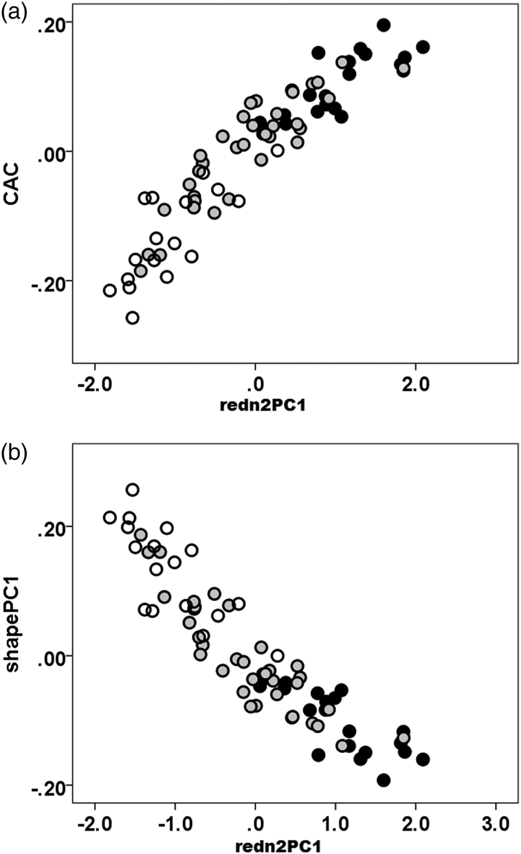
LGM analysis using geomorph yields CAC as a measure of degree and pattern of allometry. Combinations of the tip angle, ratios of orthogonal dimensions (L/T, M/T), and size variables (lnCS, mass) yield a single major dimension of variation that clearly is allometric as well and that correlates strongly with CAC. What is more, although LGM analysis is necessary to compute lnCS, most other variables are more easily obtained. An allometric component can be extracted not only from LGM data but also from other analytical approaches using easily obtained geometric, size, and ratio variables.
Discussion
This study involved Folsom replicas; similar earlier studies involved Clovis or similar points. Obviously, Folsom and Clovis points shared fluting and chronological proximity but differed in salient technological and organizational respects (Collins Reference Collins and Amick1999; Sellet Reference Sellet, Robinson and Sellet2017) that complicate comparisons. If, compared to Folsom points, “Clovis points . . . sustain many more episodes of resharpening” (Sellet Reference Sellet, Robinson and Sellet2017:271), then allometric resharpening effects in Folsom replicas suggest at least their equal probability in Clovis technology. Broadly, the generally larger size and lower launch velocity of hand-thrown spears and atlatl-launched darts extend their use life or survivorship; although such points suffer damage and edge dulling, damage is less likely catastrophic, so spear or dart points are more often subjects of resharpening than are late prehistoric arrow points that tend to fail catastrophically (Loendorf et al. Reference Loendorf, Rogers, Oliver, Huttick, Denoyer and Kyle Woodson2019:354; cf. Lerner Reference Lerner and Shott2015).
Allometry must be sought either using LGM data or ILDs, as in our study, or the allometric ratios used in earlier work (e.g., Andrefsky Reference Andrefsky2006; Lerner Reference Lerner and Shott2015; Shott et al. Reference Shott, Hunzicker and Patten2007). As earlier, IBR as an allometric measure did not pattern with reduction stage nearly as well as did tip angle, L/T, and M/T, perhaps because both stem and blade modules usually were reduced (if disproportionately). Reduction of both modules has been invoked to explain what is considered the absence of allometry in other fluted-point samples (Buchanan and Collard Reference Buchanan and Collard2010). However modules were defined and in whatever way degree of reduction was gauged there, our analysis included explicit modularity tests. Hunzicker's experimental design also provided independent control over the degree of reduction. Results suggest strongly that allometry registers even when both stem and blade modules are subject to resharpening. The key issue is testing: if allometry and especially modularity do not characterize datasets, that negative conclusion will emerge in valid tests for their effects. If the one is not considered and if neither is measured directly, negative conclusions remain ambiguous. Practically, testing must start from the hypothetical definition of at least two modules, blade and stem, and perhaps additional ones, such as tip area, per results of González-José and Charlin's (Reference González-José and Charlin2012) study. At least some modules, like stem versus blade, are easily enough defined in stemmed or notched points but possibly also in lanceolates by, for instance, the distal extent of edge grinding.
In these data, size and shape are not separated easily. As results showed, shapePC1 patterns clearly with size. In resharpened stone tools, a change in shape occurs in significant part because of a change in size, as it does in growth trajectories in many biological taxa. If “size-related shape effects are inextricably mixed up with almost every biological feature of organisms” (Oxnard Reference Oxnard1978:233), no less seems true of the morphometric features of stone tools. When allometry occurs, separating shape from size is complicated by their integral covariation. Size–shape correlation is a legitimate dimension of patterning in reduced stone tools, not necessarily an artifact of analysis.
LGM analysis of the size and shape of adults and juveniles of many animal species reveals similar patterns, with allometric change occurring as a function of growth. Conducting LGM analysis of any single species that omitted juveniles would reveal more legitimate size-free shape variation. Yet many biological LGM studies of size and shape involve sets of often related animal species and are designed to reveal and quantify differences in adult size and shape. Presumably, such studies take care to omit juveniles, because their inclusion could confuse intraspecific growth allometry with interspecific evolutionary allometry. Again, stone-tool reduction allometry works in the opposite direction of biological growth allometry; analysis seeking it must include specimens distributed along the full range of joint size–shape variation. Similarly, any analysis that distinguishes point types must control for reduction allometry within the types so as not to confuse it with design variation between types. This can be accomplished by confining LGM analysis to stems only (e.g., Prentiss et al. Reference Prentiss, Walsh, Skelton, Markes and M.Straffen2016), even if results suggest that stems themselves are subject to some allometric variation because progressive use and resharpening cause bases to intrude on them or by extracting CACs from each type before comparing types.
Finally, modularity and integration may pertain to more than the allometric trajectories that individual points take in their use lives. In the longer term, they may help explain the morphological transitions by which some types emerge over time from earlier ones (i.e., Klingenberg's evolutionary allometry). For instance, changes in the range of target species, in hunting methods (e.g., ambush versus stalking), or in the econometrics of hunting (e.g., the relationship between search and pursuit time as animal communities change) could prompt adjustments to the size and shape of stems and other modules to accommodate the changing demands of weapons range, accuracy, or thrust. Over time, such adjustments may gradually transform notched points, for instance, into stemmed ones as bases progressively narrow, necks widen, and stem margins converge toward points’ longitudinal axes. This is not to argue that all point types morphed into other types, but morphing is a possibility—a hypothesis—that LGM analysis is well suited to test.
Conclusion
Our study applied LGM methods to 3D models of 25 Folsom replicas from Hunzicker's (Reference Hunzicker2005) work. The experimental design furnished an independent control that enabled us to identify allometry with reduction. After defining separate blade and stem modules, analysis in geomorph indicated modularity; separate stem and blade modules are somewhat decomposable yet remain partially integrated. Results also indicate allometry: a change in shape with the change in size. The controlled nature of the experiment—we know how and why points underwent reduction and to what degree—conclusively identifies reduction allometry as the explanation. 3D Folsom models register both allometry and modularity in the reduction of points. With cycles of use, repair, and reuse, points change in shape as their size declines, partly because stem and blade modules experience different rates and patterns of reduction.
But ours is a controlled experimental dataset. However useful it may be in documenting both modularity and allometry and in explaining their expression, it does not provide the explanation for those features that may be observed in archaeological data. Further tests are required in a range of point types that include but are not confined to lanceolates. Archaeological datasets vary not only in typology but also in other ways (e.g., knapper, tool stone, circumstance, time) controlled for in this experimental study; the strong signals found here may be complicated elsewhere. Our study's chief value is to document the clear modularity, limited integration, and strong allometric signal that reside in these experimental data. If archaeological data pattern similarly, their parsimonious interpretation implicates resharpening as the source of the patterning.
Whether in 2D models of point outlines or 3D models of their fuller form, we should not treat all points as integral wholes. If they are indeed such wholes, valid analysis will reach that conclusion. If they display modularity and if variation among them can be attributed to reduction allometry, then valid analysis will reach that conclusion instead. Whatever the case, we must seek and test for allometry, modularity, and integration directly, rather than approaching them indirectly. At least for some purposes, points are not irreducible wholes but things of modular parts. Our analyses must recognize and exploit this modular quality.
Acknowledgments
David Hunzicker kindly provided replica casts. Brian Trail assisted in the scanning process. Robert D. Lassen kindly provided data on Folsom specimens analyzed in his 2016 article. We thank Shane Miller and two anonymous reviewers for constructive comments.
Data Availability Statement
Supplemental Tables 1 and 2 and the R Code to create Figure 6 in the text are available at the Open Science Framework (OSF) site, https://osf.io/acbs5/?view_only=2c0f225ed93d4751ad9415054d8837d0.



