


Introduction
The use of Geos-3, Seasat, or Geosat altimeter measurements over Antarctica and Greenland give major information for use in glaciological studies. From the three classical altimetric parameters (transit time, width of the leading edge of the radar wave forms, and total intensity of the received energy), such different geophysical parameters are provided as topography (e.g. Reference Brooks, Campbell, Ramseier, Stanley and ZwallyBrooks and others, 1978; Reference Zwally, Bindschadler, Brenner, Martin and ThomasZwally and others, 1983), or wind intensity (Reference Remy, Brossier and MinsterRemy and others, in press). Here, we will study the altimetric height as given by the Seasat altimeter over East Antarctica.
The topography of continental ice is useful for models of ice-sheet flow, for climatic surveys, or for undulation studies. Ice-sheet topographies have been derived from Geos-3, Seasat, and Geosat data Reference Brooks and Norcross(Brooks and others, 1982, Reference Brooks, Williams, Ferrigno, Krabill, Oliver, James and Jago1983; Reference Zwally, Bindschadler, Brenner, Martin and ThomasZwally and others, 1983, Reference Zwally, Judy, Brenner and Bindschadler1987). The error estimation is as important as the topographic map itself. Up to now, the error has been estimated, mostly from internal consistency checks, at around 1 m. These estimates do not adequately take into account the error in the orbit nor the errors introduced by the slope of the ice surface. The objective of the present note is to propose, implement, and test a technique to derive reproducible ice-sheet topographies and their error estimates. We will show that precision of less than 1 m is achievable with Seasat data. It is therefore suggested that the long-term evolution of ice-sheet topographies can indeed by estimated from satellite data.
In the first section we discuss the various sources of error in satellite-altimeter measurements. The second section explains how unbiased estimates of the topography and its error can be obtained by an inverse technique. It relies on a priori covariances of the expected parameters and realistic estimates of the measurement errors which are described in section 3. The slope-error correction is further discussed in section 4 and an optimized technique to correct this error is proposed. The method is then tested on small parts of the Antarctic ice sheet, and applied to Terre Adélie, using Seasat data (section 5). Further possible improvements and the consequences of the results are then discussed in sections 6 and 7.
1. The Errors of Satellite-altimeter Measurements over Ice Sheets
A radar altimeter transmits pulses toward the sub-satellite point and receives the returned signal, after reflection at the surface (see, for example, Reference MacArthurMacArthur, 1978). The transit time of the signal will provide the altimetric height. Three kinds of distinct errors affect its estimation.
a. The measurement error
This is the error in the distance between the satellite and the nearest point of the ice surface. The main difficulty arises from a correct estimation of the first return time of the signal, because return wave forms cannot be accurately described by a simple analytical model such as Reference BrownBrown’s (1977). Also, as the distance to the surface varies quickly, the tracking system (which pre-positions the receiving window based on previous measurements) cannot follow the variations in height, and consequently (in the case of Seasat) the on-board estimate of height is inaccurate. A re-estimation of this height, named “retracking” must be applied. Reference Brooks, Williams, Ferrigno, Krabill, Oliver, James and JagoBrooks and others (1983) proposed to estimate the return time of the signal as the time when the received energy is 50% of the maximum return power. Reference Martin, Zwally, Brenner and BindschadlerMartin and others (1983) fitted a functional, derived from Brown’s model, to the altimeter wave form for retracking. Reference Remy, Brossier and MinsterRemy and others (in press) deduced the position of the middle of the leading edge from the total energy. The last method, tested on repeat profiles of the Seasat altimeter data, provides a reproducibility of 50 cm r.m.s. This method, which is easier than that of Martin and others and more reproducible than that of Brooks and others, will be used here. Reference Ridley and PartingtonRidley and Partington (1988) recently suggested that volume retrodiffusion from the ice affects the wave forms of a radar altimeter. In this case, the height, with any retracking technique, would not correspond to the ice surface but to a level somewhat below (of the order of 1 m). This effect still requires further studies.
In addition to the estimate of the transit time of the signal, effects of propagation through the atmosphere should be considered. As the troposphere above continental ice is very dry (less than 1 g/cm2 of water vapor), the so-called wet tropospheric corrections can be neglected (see, for example, Reference Tapley and RosboroughTapley and others, 1985). On the other hand, a dry tropospheric correction should be applied, related to the pressure at the surface.
This correction, for an altitude varying from 1000 to 3000 m above sea-level, varies from 1.9 to 1.4 m (Reference SaastromoinenSaastamoinen, 1972). An additional correction related to meteorological pressure variations should in principle be applied: a 20 mbar difference induces a 4 cm difference. In the absence of reliable meteorological data, at the date of the measurements, we have only applied the pressure correction related to altitude. Finally, the effect of the ionosphere is estimated from models of the total electron content, which is quite uncertain in auroral belt areas (see, for example, Reference Lorell, Colquitt and AnderleLorell and others, 1982). A long wavelength residual error of the order of 30 cm in the altimeter value can be expected from this uncertainty. In what follows, it will be assumed for simplicity that this error is “absorbed” in the orbit error of similar wavelength.
b. The orbit error
This is the uncertainty in the radial position of the satellite. The satellite ephemerides are computed from the dynamic laws of motion combined with laser- or doppler-tracking data. The accuracy of the nominal orbit over high latitudes is probably worse than over temperate regions because of the lack of tracking stations and of the relatively larger error in existing geopotential models. For Seasat, this error is of the order of 70 cm r.m.s. (Reference Lerch, Marsh, Klosko and WilliamsonLerch and others, 1982). A value of 1 m will be used here. The orbit-error spectrum is dominated by the one cycle per orbit revolution “free” frequency of the satellite. This allows us to represent the radial orbit error along each altimeter profile of length less than 10 000 km by a linear or quadratic polynomial fitted in order to minimize the height departures from the other crossing profiles. This procedure is frequently applied as a preliminary step before mapping oceanic or ice-sheet topography.
However, this inexpensive method of orbit-error reduction does not satisfy the requirement of high-accuracy mapping. It does not take into account the high correlation between the error in two successive arcs. Also, it has recently been recognized that a non-negligible fraction of the orbit error only depends on the geographic coordinates. This part of the radial error cannot be removed by the crossing-arc analysis and is mapped within the topography (Reference Tapley and RosboroughTapley and Rosborough, 1985; Reference WagnerWagner, 1985; Reference MazzegaMazzega, 1986). This difficulty is overcome by the inverse method of data analysis adopted in the present paper: the description of the statistical properties of the orbit error by a time-autocovariance function naturally specifies its space correlations (see, for example, Reference Bretherton, Davis and FandryBretherton and others, 1976; Reference MoritzMoritz, 1978). For altimetry, this approach has been pioneered by Reference ZlotnickiWunsch and Zlotnicki (1984) in a sensitivity study using a set of simulated altimeter tracks. It has recently been extended by Mazzega and Houry (1988) to the determination of the Mediterranean mean sea-level from Seasat data. This paper is the first attempt to obtain regional topography of the Antarctic ice sheet by inversion of the altimeter data.
c. The slope-induced error
The altimeter measures the distance to the nearest point of the surface, within the radar footprint (Fig. 5a). Because of the slope of the surface and because of the large size of the footprint, the impact point can be as far as a few kilometers from the nadir point. The difficulty is that the position of the nearest point is not known a priori. If it is assumed to be at the (known) nadir position, an error of the order of several tens of meters is introduced for typical ice-sheet slopes of the order of 0.5°. Two correcting methods have been proposed by Reference Brenner, Bindschadler, Thomas and ZwallyBrenner and others (1983): the “relocation method”, which estimates the true impact point, and the “direct method”, which consists in estimating the height for the nadir position. Here, we will generalize this point of view and propose a method which should minimize the residual error after correction. This method will then be used in the inverse calculation of the topography. In brief, the situation of altimeter errors over an ice sheet is very different from that over the ocean. For the latter, the measurement error is of the order of a few centimeters and the “slope error” is negligible, so that orbit errors dominate. Above continental ice, in the case of Seasat and probably ERS-1, the measurement error and the orbit error are similar, of the order of 50 cm to 1 m, and the slope error dominates.
a. Geometry for the slope error. The impact point I of the radar wave form is shifted along the maximum slope with respect to the nadir N. The induced altimetric height h will be too high. There is a point M between N and I such that its altitude is the measured one. b. Geometry of the altimeter measurement. f(x) is the real profile along a maximum slope section; g(x) is the measured one. The impact of the radar pulse is al a distance δx from the nadir such that the range H is minimum. In the intermediate method, one searches for the point where the real range is H. It is at a disantce ρ from the nadir. The height correction с in the direct method is the difference between g(x) and f(x) at the nadir.

2. The Inverse Method of Ice-Sheet Mapping
The data used for this study are the Specialized Data Record (SDR) of the Seasat altimeter. They consist of an altimeter return wave form every 0.1 s, corresponding to an along-track resolution of 670 m. The data-set coverage is shown in Figure 1, and is enlarged for the test areas in Figures 6a and 7a. The retracking technique (Reference Remy, Brossier and MinsterRemy and others, in press) is first applied to these wave forms. To reduce the noise and the number of data, averages over three consecutive 0.1 s retracked heights have been performed, leading to a 2 km along-track resolution.
Map of the Seasat altimeter data over Antarctica used in this study. The three areas A1, A2, and B which are mapped in Figures 6–13 are also indicated.

Treatment sequence as explained in the text for area A1 shown in Figure 1. We select tracks (a), calculate a mean surface (b), map the residual surface by the inverse method (c), add it to the mean surface (d), estimate the a posteriori error (e), and correct the slope error (f).


The altimeter data d(r,t) taken at the geographical position r(.x,y) and at time t are related to the height h(r) of the ice-sheet topography relative to the reference ellipsoid by the following relation:

where e1 is the instantaneous instrumental error, еоrЪ is the radial component of the orbit error, and eslo(r) is the slope-error correction.
The reconstruction of a high-accuracy map of the ice sheet from these complex measurements is not straightforward: the data coverage exhibits large gaps as well as local oversampling; the orbit error eorb has quasi-periodic correlations in time, whereas the instrumental error is almost a white noise (see section 3). Finally, the slope-error correction eslo(r) is related to the local maximum gradient of the topography h(r) itself. We consider the ice topography h(r) as consisting of the superposition of two independent components (see, for example, Reference McIntyre and DrewryMcIntyre and Drewry, 1984), say:

h0(r) is the large-scale shape of the ice sheet, with kilometric amplitudes, corresponding to the average shape of the ice sheet. In a first approximation, it can be represented by a two-dimensional functional of geographic position fitted to the data in a preliminary step (see section 3). The resulting surface is then used as a first guess to analyse the reduced data d(r, t) — h0(r). The latter are dominated by short-distance scale undulations created by the flow of ice over the bedrock rugosities. This separation can be well justified by along-track wave-number spectra of the altimeter profiles.
The quantities δh, e1 and eorb are considered as the results of stochastic processes. We anticipate their statistical properties by specifying their covariance functions, respectively Ch, C1, and Corb . Using the least-squares criterion, the optimal estimation of the residual topography δĥ at any location r(x, y) is obtained by a linear combination of the reduced data including the covariance functions (Reference Tarantola and ValetteTarantela and Valette, 1982; Mazzega and Houry, 1988):
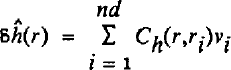
where nd is the number of data and ν;• is given by:

The (i, j) element of the symmetric definite positive matrix S is constructed by:

The height of the ice topography above the reference ellipsoid is then:

with an a posteriori covariance computed from the relation:

where the term A(r, r) is the information gained from the data analysis:

The use of the various covariance functions in Equations (3), (4), and (5) ensures uniqueness and stability of the inverse solution ĥ(r). In the limiting case of perfect data sampling (in space and time as the covariances show both dependencies), the optimal map ĥ(r) would not depend on the first guess h0(r). Conversely, in the regions of large data gaps, the final map ĥ(r) and its variance  tend respectively to the a priori map h0(r) and the covariance of the topography Сh(r,r). The following section is devoted to the estimation of the starting map h0(r) and to the choice of the a priori covariance functions Ch1, C1, and Corb
which (with the altimeter data set) determine the optimal solution h and its accuracy.
3. The Mean Surface and the Covariance Functions
a. Choice of the mean ice-sheet surface
In the case of the mean sea surface, the reference surface can be derived from independent estimates of the geoid and dynamic topography, derived from gravimetric data, and hydrography. Here, the existing independent ice-sheet topographies are either much less precise than altimetric data or provide too little coverage (Reference McIntyreMcIntyre, unpublished). Hence they do not provide a useful initial reference. We will derive the latter from the data themselves, using an a priori description of the ice topography.
Indeed, if the ice sheet is assumed to be perfectly plastic in steady state and frozen to a flat bed, its surface is given by:

where z is the height at a distance d from the center of the ice sheet, Z and L are the maximum reference height and horizontal distance from the center (Reference PatersonPaterson, 1981). If one writes equation (9) with Cartesian coordinates, and neglecting the variations in z2 compared to the variations in z4, one can show that z4 can be written as a second-degree polynomial.
For an arbitrary altimetric profile, if one assumes that the satellite path is rectilinear, the surface height above the reference ellipsoid will then be:

where x is the along-track distance.
We will use this description of the large-scale topography to estimate the reference surface. The difficulty with this approach is that it will be contaminated by the as yet uncorrected slope errors. This will also affect the residual heights above this reference. For a large surface, this difficulty will be overcome by an iterative approach.
As shown in Figure 2, relation (10) fits plainly the large-scale pattern of altimetric profiles. The residuals are dominated by meso-scale undulations of amplitude 4 m and wavelength 20 km, which correspond to “type 2 surface features” as named by Reference McIntyre and DrewryMcIntyre and Drewry (1984).
Treatment of an altimetric profile before inversion. Fitting of a parabolic surface (a), extraction of the residual altimetric height (b), and calculation of the along-track covariance functions of residual heights (c).

Using a least-squares analysis, we therefore fit all the retracked altimeter data to a two-dimensional quadratic form. This was done for areas A1 and A2 (Figs 6b and 7b). The mean r.m.s. for all altimetric profiles in these areas is 3.5 m: for this scale (͌100 km), the near-parabolic surface fits the data very well and the induced surface should be a good reference. The larger the scale is, the less impressive the fit should be. Indeed, the mean surface of area B (Fig. 10) cannot be correctly represented by this technique. We will return to this in section 5c.
Topography of area B (Fig. 1) using several techniques: (a) by aircraft in 1974; (b) adapted from the Canadian Bathymetry chart of Ocean, in 1980; (c) by balloon in 1982; (d) by radar altimetry (Reference Brooks and NorcrossBrooks and Norcross, 1982); (e) here, by radar altimetry for the first inversion (see text). The second inversion is shown in Figure 11. The (a-d) figures are adapted from Reference Brooks and NorcrossBrooks and Norcross (1982).

b. Choice of covariance of the model parameters
The model parameters (the residuals) are only space-dependent. The covariance function expresses the behaviour of h(x, y) relative to a shift δх,δу:
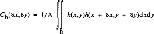
where A is the area of the domain D.
Undulations, which dominate the residuals, are thought to be elongated along the ice-flow direction and are altitude-dependent (Reference McIntyre and DrewryMcIntyre and Drewry, 1984). Thus, Сh(δх,δу) is neither stationary nor isotropic. Although it is theoretically feasible to construct the correct covariance matrix, we will assume, as is usually done, that it is stationary (i.e. independent of position) and isotropic (i.e. identical in all directions).
In Figure 2c, the calculated correlations of the residuals along an altimetric profile show a large component expressing the behaviour of the residuals on wavelengths of the order to 20 km, superimposed by a smaller sinusoidal component. The latter should express the behaviour of the residuals on short wavelengths. When several profiles with different undulations are mixed, this component disappears. It will therefore be neglected in further calculations. The presence of a negative lobe is very constraining: a particular point, not sampled by the altimeter, but situated at about 80 km from the satellite tracks, should have a residual height which is very strongly constrained by the data. This is probably related to the regularity of the undulations.
Using purely empirical correlation functions generally leads to unstable matrix inversions in equation (4). One should rather fit a theoretical covariance function to an empirical one. If undulations are described by Gaussian functions like the “bell-shaped mounts” of Reference McIntyre and DrewryMcIntyre and Drewry (1984), the covariance function will also be Gaussian. In further calculations, we selected a semi-empirical covariance by fitting a Gaussian one to the positive part of the empirical covariance (Fig. 3). The amplitude is the mean variance of the residuals (3.5 m)2 and the characteristic decorrelation length is 9 km.

δ is in km and Ch in m2.
Averaged empirical correlation function of the parameter superimposed on the Gaussian function used for the inversion. The variance is 12 m2.

While doing so, we a priori lose some of the information contained in the data, which were described by the negative lobe of Figure 2c. One of the reviewers suggested that a scale-invariant model (Poisson type) should be more adequate in view of the observations. Though this suggestion seems appropriate, we have not used it, as this work is mostly a demonstration of the approach.
c. Covariance of the errors
The instrumental error, after retracking, can be considered a white noise of 50 cm r.m.s., as tested by the comparison of repetitive altimeter profiles (Reference Remy, Brossier and MinsterRemy and others, in press). Thus, the covariance C1 will be a Dirac-delta function of amplitude 0.25 m2. This should overestimate the noise of the three-point mean values.
The Seasat orbit was calculated as consecutive 6 d independent arcs. The orbit error is dominated by frequencies around 1 cycle/revolution due mainly to errors in the gravity field and erroneous initial elements in the orbit integration (Reference WagnerWagner, 1985). Reference ZlotnickiWunsch and Zlotnicki (1984) suggested that the orbit covariance error can be described by a cosine with an exponential dumping:

where δt is the time lag between two data points, σ2 orb is the orbit error variance, here set to (1 m2), and T ≈ 101 min is the Seasat orbital period. δT is a characteristic decorrelation time, about five revolution periods (Fig. 4). The autocorrelation between two points belonging to independent arcs is set to zero. This description could easily be improved once a better orbit-error description becomes available. In particular, short wavelength orbit errors are not well described by this functional.
Autocorrelation function of the Seasat radial orbit error. The decorrelation time is for five revolution periods, and two points belonging to independent arcs are taken as uncorrelated.

Thus, the complete data error covariance C defined by:

quantifies the confidence we have in each datum.
4. The Slope-error Correction
In all that follows, α will be the maximum local slope. Whenever it is deduced from the data, this means that it is deduced from the two-dimensional maps as estimated using the inversion technique.
a. Problem: geometrical approach
The impact point of the radar wave front, which is the nearest point from the satellite, is shifted from the nadir N as soon as a slope exists (Fig. 5a).
The measured range (H) is too small, compared to the nadir distance, so that the apparent ice elevation h, above the reference ellipsoid, is higher than the real one hN :

On the other hand, this apparent height h is smaller than the real height at the impact I:

For correcting this effect, Reference Brenner, Bindschadler, Thomas and ZwallyBrenner and others (1983) proposed two methods: in the “direct” method, the measured range of the nadir is estimated by subtracting the error term α2H/2. In the second method, named the “relocation” method, the location of the impact point is estimated and the height of this point corrected by adding the error term. For both cases, the slope being deduced from the data, an iterative scheme is used. It is clear that these methods are the two extremes of a range of possibilities.
What we propose here can be called an “intermediate” method. From Equations (15)-(16), one can see that there is a unique point between the nadir and the impact, for which the range measurement H is the correct one. The horizontal distance between the nadir N and this point M is:

We propose to search for the location of point M. This is easier than using the “relocation” method, because only the position has to be corrected. Also, we will show in section 4b that the residual error after correction is smaller in the “intermediate” method than in the “direct” one.
b. Residual errors: analytical approach
In this section, we evaluate the residual second-order error after the slope correction in the various methods.
Let us consider f(x) as the real ice-surface height along a maximum slope section. The measured range H is the distance between the satellite and the surface at a position χ + δx such that H is minimum. This provides an apparent profile g(x). To the second order:

If the curvature f”(x) is negligible, one finds relation (15). However, Hf” is not necessarily small above the ice sheet.
In the direct method, the real correction с should be the difference between g(x) and f(x), that is:

where the derivatives are calculated at position x.
As the slope is deduced from g(x), the correction c* which is actually made is:

By derivation of relation (18), one obtains a second-order residual error after slope correction:

In the intermediate method, one is looking for the position x + ρ such that the actual range is the measured one H. Thus:

From Equations (22) and (18), one derives the “real” value for ρ (to the second order):

The residual error after the slope correction in the intermediate method can be estimated either as a position error or an a height error. The actual position correction, from equation (17) is:

Therefore, the residual position error is:
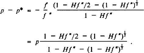
Note that the error will be of the third order if Hf” is small. Alternatively, it can be stated that the real height at position x + p* is:

whereas the method attributes a height g(x) to this position. Hence, the residual height error after the correction is:

By comparing Equations (21) and (27), it is apparent that the residual height error after slope correction is twice smaller using the intermediate method than by using the direct method. This difference will be the same at each iteration. Note also that Equations (21) and (27) are of opposite signs, с — c* is of the opposite sign to f”, which is, because of the curvature of the parabolic profile, often negative: the direct method will tend to smooth the undulations. On the contrary, the intermediate method will tend to amplify these undulations.
In order to get orders of magnitude of these effects, imagine that f(x) is an undulation of strong amplitude, 14 m, and of wavelength 20 km

x is in kilometers and f is in meters. Hf”, for H = 800 km, is of the order of 0–0.5 and cannot be neglected in equation (18). Then, at the first iteration for x = 3 km, с = 0.65 m, and с – с* = 0.21 m, ρ* = 355 m and ρ – ρ* = 30 m.
For x = 0, c = 1.93 m, and с – с* = 0, ρ* = 880 m and ρ — ρ* = 0.
The large-scale slope effect is of the order of с ≈ 1.5 m for a slope of 0.1° (e.g. in Figure 2, the large-scale slope of 0.06). ρ is then of the order of 700 m.
c. Insertion of the error correction in the inverse method
Reference Zwally, Thomas and BindschadlerZwally and others (1981) argued that a similar altimeter will give the same slope error so that it is not necessary to correct for it. This is only true to the extent that a dense enough coverage of observations is achieved. Even then, however, the separation of the measurement positions will be of a few hundreds of meters, so that the actual slope error will differ by a few tens of centimeters. This is close to the required accuracy for monitoring the climatic evolution of ice sheets. Also, if the actual distance between undulations and their relation to the bedrock are studied, it is necessary to correct the maps for the slope error.
The previous discussion uses the maximum slope. Because of the altimeter sampling, the slope can be fairly well estimated along-track, but it is more poorly known across-track. For this reason, Reference Brenner, Bindschadler, Thomas and ZwallyBrenner and others (1983) estimated the local slope along-track (which is dominated by undulations; see Figure 2) and the large-scale slope across-track. Using the inverse technique, the slope can, in principle, be derived directly from the a priori covariance (equation (3)) or directly from the solution. Of course, in the latter case, the error in the estimated heights, and therefore in the estimated slope, will not be the same everywhere. However, the technique provides an error map, so that this could be taken into account. In what follows, we show how we used the slope correction in the inverse calculation. equation (3), giving the residual solution, is applied at a grid point (i, j). The grid spacing s is chosen as 2 km: this is compatible with the along-track sampling and is adapted to the scale required for slope estimation. From equation (3), the slope for residuals δh(r) is:

where vk is defined in equation (4). To the residual slope, on the i and j directions, one should add the mean surface slope. This provides the slope α as defined previously, so that equation (17) can be applied to the data points. In this work, Equations (3) and (4) were iteratively applied without modifying S−1, in order to decrease the computation cost. Obviously, from this point of view, it would be easier to apply the direct method for slope correction, as S would be strictly constant, and only d(r¡,ti) would have to be changed in equation (4) at each iteration. On the other hand, in view of the expected values of p, which are an order of magnitude smaller than the radar footprint and the undulations' half-wavelength, the expected modification of the S matrix is small.
5. Ice-sheet Mapping
a. Mapping the test areas
As a test, the method is first applied to two small overlapping areas (named A1 and A2 in Figure 1).
Figures 6 and 7 show the complete treatment sequence: (a) selection of altimetric tracks; (b) calculation of the mean surface; (c) calculation of the residual altimetric height using the inverse method; (d) reconstruction of the topography; (e) estimation of the error; and (f) correction of the slope error, estimated by one iteration.
On the residual maps, undulations a few meters high and a few tens of kilometers in length can be identified. Note that most of the track interruptions, which can been seen in Figures 6a and 7a, occurred where these undulations are important (see Reference Partington and RapleyPartington and Rapley, 1986). The slope-error correction mostly modifies these undulations (Figs 6e and 7e). For area A2, some undulations are shifted up to 4 km.
The error result is not unexpected: at a maximum (equal to the input variance, here set to 12 m2) for those areas of poor data density, and at a minimum for those areas of high data density, for instance near lat. 72°S. Near crossing tracks, the error is of the order to 40 cm. To this error, one should add the residual error of slope correction. From section 4, it should be of the order of 0.2 m r.m.s.
b. Tests
The area between lat. 72° and 71.5° S., and between long. 105° and 102.5 °E. is mapped in both Figures 6 and 7. The difference between the two maps (Fig. 8) reaches 3 m along the boundary due to border effects. Half of the surface is reproducible within 1 m, which is compatible with the error maps.

For such small areas, none of the altimeter tracks were covered on the same day. Hence, one of the most significant benefits of the method, which is to handle accurately the orbit-error spectrum, was not used in these tests.
As a further test, we underestimated the a priori variance by taking a value of 3.5 m2 instead of 12 m2. The result is illustrated in Figure 9. This produces a tilt in the surface. What probably happens is that less flexibility is allowed for the surface to adjust itself through undulations, so that the inverse calculation essentially modifies the reference surface.
Difference between inversion shown in Figure 6d and inversion where the variance of the parameters is underestimated at 3.5 m2 instead of 12 m2.

Mazzega and Houry (1988) provided other tests for the technique, as applied to the mean sea-surface estimation.
As a whole, these tests raise confidence in the method. The error, in places with sufficient data, is of the order of 0.5 m r.m.s. This is encouraging.
c. Terre Adélie map
In this section, we map a region of 300 km by 500 km chosen around the line from Dumont d'Urville to Dome C (Fig. 1), where the data could be useful to many expeditions. The method is consuming of computer time, because of the inversion of a square matrix, the dimension of which is equal to the number of data. Therefore, a complete map of Antarctica (to the north of lat. 72° S.) would be achievable only with array processors.
As is shown in Figure 10, the mean surface cannot be approximated as explained in section 3a. In order to overcome this difficulty, we used an iterative scheme. This is possible because the topography is a simple combination of two dominant wavelengths. Figure 10e is obtained from a reduced set of data (15%) using the inversion method. The variance is set to (2000 m)2 because the range of heights is between 1000 m and 3000 m, and the spatial radius of decorrelation is set to 140 km. This filters the undulations. This “mean” surface is very close to that of existing maps of this sector, as deduced from classical techniques (Reference Brooks and NorcrossBrooks and Norcross, 1982).
The variance of the residual altimetric profiles is about 12 m2 for areas A1 and A2. We then applied the same process as before. The resulting topography is given in Figure 11, at a 2 by 2 km2 resolution, and the error map before slope correction is shown in Figure 12. Although the data density is smaller than for the test areas, the minimum error (0.35 m) is also smaller. Because the satellite radial errors are correlated over large distances, a given point is constrained from the whole arc, which reduces the final r.m.s. errors. Even on the scale of Figure 10, important differences are obtained from the map of Reference Brooks and NorcrossBrooks and Norcross (1982). However, our retracking technique is more accurate (Reference Remy, Brossier and MinsterRemy and others, in press); we correctly take the orbit error into account, and our maps are also slope-corrected. On the other hand, we have used only a fraction of the Seasat data in this calculation: a map using more data would present a more homogeneous error map. However, the large-scale picture should be less sensitive to the additional data coverage.

6. Discussion
The error obtained here should be considered with some care, because of the number of limitations already mentioned: the retracking technique does not exactly provide the ice surface, some of the geophysical corrections leave residual errors, the orbit error is described in a somewhat schematic way, and the a priori covariance function of the signal is also quite simplified relative to the observations. Yet, the precision obtained here should be compared with expected signals.
Error map before slope correction corresponding to Figure 11. The precision is excellent (≈0.35 m) where the density of data is high.

The problem of growth or shrinkage of the ice sheet pre-occupies the climatologists, more particularly because of the potential warming of the Earth as a result of human activity. Two methods can provide additional information: survey of the topography, or measurement of the input (accumulation rate) and the output (above all iceberg discharge of water and melting at bedrock level). Up till now, precision attained using both methods does not allow evaluation of any possible change: detailed surface measurements have been obtained in a few areas, but this will not give a general trend, because of the dynamical redistribution of mass within the ice sheet (Reference Zwally, Thomas and BindschadlerZwally and others, 1981).
Because of the remarkable precision obtained over the ocean, one can also propose a sea-level survey (Reference Born, Tapley, Ries and StewartBorn and others, 1986). Due to the surface ratio, the sea-level change in relation to that of ice-sheet elevation is about 1/30. However, sea-level elevation due to climatic warming is 70% due to the expansion of warm water and 30% to ice-sheet melting (Reference Barth and TitusBarth and Titus, 1984). The actual ratio, taking into account the expansion of warm water, is hence 1/10. Until now, the best ocean-topography precision (obtained using the inverse method and Seasat data) is 11 cm (Mazzega and Houry, 1988) for the Mediterranean Sea (this precision is only relevant to wavelengths greater than 400 km, due to data coverage, but this is what is required for the present problem). With the launch of Topex-Poseidon in 1992, the precision attainable will be a few centimeters for these wavelengths (Reference Stewart and LefebvreStewart and Lefebvre, 1987). Therefore, a precision of a few tens of centimeters on ice sheets is required for the glaciologists to monitor the same signal.
The mean accumulation rate over Antarctica and Greenland is about 15 cm/year. It is of the order of a few centimeters over the summit of the ice sheet and about 1 m near the coast (Reference Zwally, Thomas and BindschadlerZwally and others, 1981). At a zero-order level of description, a 30% mass imbalance would cause an ice-sheet surface diminution of 50 cm over a decade. The precision required to observe this effect is of the order of a few centimeters above the summit of the ice sheet or of 1 m near the coast.
The slope error of the classical radar altimeter is important where the required precision would be accessible. In order to overcome this difficulty, we suggest monitoring the elevation of Antarctic “lakes”. They are only a few tens of kilometers in size and probably correspond to valleys in the bedrock (Cudlip and Mclntyre, 1986). For example, Astrolabe Lake clearly appears in Figure 11. It is enlarged in Figure 13a. Up to 70 consecutive SDR measurements are within 1 m of height. Thus, the middle of the lake should be free of slope error. The propagated error (Fig. 13b) is of the order of 40 cm in this area. The measurement of accumulation rate is about 10 cm/year from in-situ data, and between 20 and 30 cm/year when derived from the microwave emissivity at 31 GHz (Reference Rotman, Fisher and StaelinRotman and others, 1982). A mean value of 20 cm/year and a 30% mass imbalance would give a change of 90 cm in 13 years (the time interval between Seasat and ERS-1). Of course, the whole dynamics of the ice sheet would have to be considered in addition to this purely local effect. Anyway, 1 m change is likely to be larger than the error bars. Such “lakes” are not rare in Antarctica (one can find several in Figure 11). A systematic survey of all available lakes would provide a general trend of the ice sheet.
Enlargement of the square drawn on Figure 11, around Astrolabe Lake, (a) Topographic map; (b) Error map, free from significant slope error.

Finally, in addition to these height changes, if volume echo affects the signal of altimetric height, changes could also result from changes in the ice grain-size, which are related to the accumulation rate (Reference ZwallyZwally, 1977; Reference Ridley and PartingtonRidley and Partington, 1988).
7. Conclusion
Because of computer limitations, our results are not yet optimal. Dividing the domain into separate regions would give the calculation shortcomings inherent in the data set: correlated errors would be treated as independent. Handling small matrices, by taking into account only the data surrounding the prediction point, would also be inadequate for the same reason. The method has to be used on a high-speed and large-memory computer in order to invert the whole data set.
We have developed a new method for slope-error determination which converges quickly and leads to a small residual error, but we have not correctly evaluated the latter. The inverse method constitutes a flexible tool to mix data of different natures by the use of cross-correlations. For example, the local variations in the total energy return of the altimeter are linked to the absolute slope (Reference Remy, Brossier and MinsterRemy and others, in press). Since these data are simultaneous, this information could be introduced, as well as the slope-correction equations, directly into the calculation. The a posteriori error would also, in this case, take into account the slope error.
This method should be well adapted to the ERS-I data, which will provide a wide and dense coverage up to lat. 82° S. Its radial orbit error should be of the same order as that of Seasat. It should benefit from present progress in geopotential models. If a tracking station could be installed near the ice sheet, orbit error would locally be considerably smaller. We have shown that the a posteriori error should then reach 0.35 m, depending on the data distribution and the local slope. This suggests that after the launch of ERS-I one should be able to detect possible climatic variations in the ice sheet.
Acknowledgements
All of the scientists of the Groupe de Recherche de Géodésie Spatiale are thanked for their discussions, and the stimulating environment. Comments by the reviewers were found to be very constructive and helpful.



