




1 Introduction
The swash zone, or the region of the beach that is continuously covered and uncovered by wave runup, is a unique example of an environmental flow in which sediment suspension can be observed even when the mean velocity of the runup is not sufficient to generate shear stress capable of mobilizing the sediment in question. The uprush and backwash phases are fundamentally different flows (Petti & Longo Reference Petti and Longo2001). Sediment transport in the backwash consists primarily of sediment transport via bedload and relates well to predictions from Shields (Reference Shields1936), in which mean shear at the fluid–sediment interface generates a turbulent boundary layer and causes dislodgement of the sediment grains. On the contrary, uprush is more accurately described as bore-advected turbulence (Butt & Russell Reference Butt and Russell1999; Puleo et al. Reference Puleo, Beach, Holman and Allen2000; Cowen et al. Reference Cowen, Sou, Liu and Raubenheimer2003) and is an example of a flow in which the near-bed turbulence does not result solely, or even primarily, from the mean flow, thus requiring a physical description that goes beyond the traditional mean flow driven bed shear stress to quantify resulting sediment transport (Nelson et al. Reference Nelson, Shreve, McLean and Drake1995).
With benthic-generated turbulence in the backwash, bed shear stress,  $\unicode[STIX]{x1D70F}$, is relatively straightforward to characterize in unidirectional flows assuming a hydraulically smooth bed; bed shear stress can be determined as
 $\unicode[STIX]{x1D70F}=\unicode[STIX]{x1D707}(\unicode[STIX]{x2202}\langle u\rangle /\unicode[STIX]{x2202}z)$, evaluated at the bed, in which
 $\unicode[STIX]{x1D707}$ represents fluid viscosity and
 $\unicode[STIX]{x2202}\langle u\rangle /\unicode[STIX]{x2202}z$ describes the bed-normal gradient of mean streamwise velocity at the bed. Whereas the shear resulting from the gradient of the mean flow produces turbulent kinetic energy, and that fluctuating turbulent energy subsequently affects local sediment motion, as in Einstein (Reference Einstein1950), the requisite critical shear stress for sediment motion remains determined by the turbulent boundary layer resulting from the mean flow rather than separate shear-driven and turbulence-driven components.
Bed shear stress can be described in relation to friction velocity,  $u_{\ast }$, where
 $\unicode[STIX]{x1D70F}=\unicode[STIX]{x1D70C}u_{\ast }^{2}$ and
 $\unicode[STIX]{x1D70C}$ denotes the density of the fluid. The latter definition is convenient in fluid flows above sediment beds when describing sediment motion that occurs as a result of a critical shear stress or critical friction velocity being exceeded. This scenario was crucial to the experiments that culminated in the famous Shields curve, shown in figure 1. The Shields curve summarizes the requisite critical mean bed shear stress, via the related critical friction velocity, for incipient particle motion for sediments of various grain sizes and specific weights subjected to unidirectional flows. Despite uncertainty in Shields’s measurement conditions and lack of clarity regarding what constitutes incipient motion, this parameterization of critical shear stress is commonly used as a threshold for sediment motion in a wide variety of applications for non-cohesive sediments in environmental and industrial applications (Buffington Reference Buffington1999).
It is also important to note that regardless of the physical mechanism that generates sediment transport, the definition of incipient motion or the initiation of motion can drastically alter the context in which results are applicable. For example, the work of Hoffmans (Reference Hoffmans2010) shows the great span of Shields parameters obtained for a single sediment type that depends upon the definition of incipient motion ranging from occasional particle motion at some locations to permanent particle movement at all locations and beyond into ripple formation; this highlights the vast uncertainty that can come from the original work of Shields (Reference Shields1936). Whereas the bed load characterizations of Kramer (Reference Kramer1935) aimed to clarify discrepancies between frequency or content of sediment transport, they are not consistently referenced for context. Further, it is important to keep in mind that sediment mobility, albeit reduced, can occur well below the threshold of critical shear stress (Paintal Reference Paintal1971); thus observations of transport do not necessarily indicate critical concurrent flow conditions in a turbulent boundary layer. Yager, Schmeeckle & Badoux (Reference Yager, Schmeeckle and Badoux2018) point out that while critical shear stress is assigned a single constant value for a given flow scenario, there are many causes for sediment to be mobilized above or below the critical shear stress, including sediment protrusion, intergranular friction and history of the flow.
Shields curve, reproduced from the dissertation of Shields (Reference Shields1936).

In contrast to sediment transport observed in the relatively uniform backwash of the swash, flow dynamics and sediment transport in the uprush behave quite differently. Despite the relatively unidirectional nature of the uprush, transport exists as both bedload and suspended load as it travels up the beach face (Masselink & Hughes Reference Masselink and Hughes1998). Turbulence levels in the runup are often dominated by offshore wave activity and consequently exceed turbulence levels that would be generated in a boundary layer of an equivalent magnitude mean flow in absence of offshore wave breaking (or an alternate source of non-boundary layer turbulence). With this additional source of turbulence, sediment movement can occur at lower mean flows than would otherwise generate sufficient stress in a uniform flow, due to intermittent instantaneous localized shear stresses, yet the amount by which the requisite critical mean stress can be effectively reduced remains poorly understood. Thus, new methods must be considered to explore the role of turbulent stresses, as compared to mean shear stresses, as they contribute to sediment transport in coastal zones. Even in the complete absence of mean shear, local and intermittent turbulent events can generate strong shear stresses that contribute to sediment pick-up (Heathershaw & Thorne Reference Heathershaw and Thorne1985). Furthermore, pressure gradients and fluctuations associated with these flows can cause fluidization of the bed and sediment motion not expected by shear alone (Foster et al. Reference Foster, Bowen, Holman and Natoo2006; Musa et al. Reference Musa, Takarrouht, Louge, Xu and Berberich2014).
In the interest of pursuing the balance between mean shear stress and superimposed turbulence, for example that of the swash zone uprush, there is a need to explore turbulent flows in which mean shear stress is negligible and stress is only imposed by turbulence. Indeed, there is a growing body of literature that explores boundary layers that result from highly turbulent flows in the absence of mean shear altogether. Common methods of considering flows with negligible mean shear include, but are not limited to, channel flows along moving beds (Uzkan & Reynolds Reference Uzkan and Reynolds1967; Thomas & Hancock Reference Thomas and Hancock1977; Hunt & Graham Reference Hunt and Graham1978), mixing boxes via active grids (Rouse & Dodu Reference Rouse and Dodu1955; Thompson & Turner Reference Thompson and Turner1975; Hopfinger & Toly Reference Hopfinger and Toly1976; McDougall Reference McDougall1979; Brumley & Jirka Reference Brumley and Jirka1987; McKenna & McGillis Reference McKenna and McGillis2004; McCorquodale & Munro Reference McCorquodale and Munro2017), stirring via jet arrays (Variano, Bodenschatz & Cowen Reference Variano, Bodenschatz and Cowen2004; Perez-Alvarado, Mydlarski & Gaskin Reference Perez-Alvarado, Mydlarski and Gaskin2016; Johnson & Cowen Reference Johnson and Cowen2018), or insertions of non-fluid interfaces in developed or developing turbulent flows (Perot & Moin Reference Perot and Moin1995a; Teixeira & Belcher Reference Teixeira and Belcher2000). Such boundary layers can generate significant instantaneous shear stresses; whereas traditional methods of determining shear stress from mean velocity gradients suggest negligible shear stress when the temporally averaged stress approaches zero, clearly instantaneous events can produce high levels of boundary stress.
Despite the breadth of literature describing the development and structure of turbulent boundary layers in the absence of mean shear, there remains a gap regarding how to identify the extreme instantaneous events that initiate sediment motion. Shear stress as it pertains to sediment motion remains poorly understood, as traditional methods suggest little transport despite field and laboratory observations of transport in turbulent flows with low relative mean shear. Whereas the Shields curve effectively characterizes mean shear stresses required for incipient motion, there is not an equivalent to the Shields curve at the other end of the spectrum, when motion is initiated by strong levels of turbulence but negligible mean shear.
Indeed, this is not a new question, as Tsai & Lick (Reference Tsai and Lick1986) recognized the ability of turbulence to suspend sediment in the absence of mean shear, and they were the first to study sediment transport in experimental studies in grid-stirred tanks (GSTs). Sediment cores from the field were placed directly into the GSTs. Tests were run until sediment in the GST was consistently suspended and entrained into the flow, and resulting suspended sediment concentrations were then calibrated to sediment concentrations generated in a flume where the bed shear stresses were determined by the driving parameters of the facility. Sediment concentrations were found to vary with the forced grid oscillation frequency, though flow statistics inside of the GST were not measured directly.
Sanchez & Redondo (Reference Sanchez and Redondo1998) continued in the same vein, performing experiments in a GST to explore the likelihood of sediment to remain entrained in a mean shear free turbulent flow. They considered suspended sediment concentrations calibrated to images of known sediment concentrations to determine the mass flux possible from a given turbulent root mean square (r.m.s.) velocity. The r.m.s. velocity was calculated from a prior formula developed by Turner (Reference Turner1968) based on the physical geometry of the GST and driving parameters of the oscillating grid.
Medina, Sanchez & Redondo (Reference Medina, Sanchez and Redondo2001) further developed the work with GSTs to study initiation of sediment motion due to turbulence to determine how the turbulent r.m.s. velocity compared with the critical velocities identified by the Shields curve. By placing a thin layer of uniform sand at the bed of the GST and altering the forced flow conditions until sediment was in suspension, they determined the turbulent r.m.s. velocity for sediment suspension. The sediment was already in suspension when the r.m.s. velocity was determined, and so incipient motion was not necessarily the standard for selecting the critical GST parameters from which r.m.s. velocities were determined for each sediment grain size. Furthermore, velocities were not measured directly, but were instead computed from the driving frequency and geometry of the GST assuming decay of turbulence away from the grid. In comparing these critical turbulent r.m.s. velocities of sediment suspension with expected critical Shields velocities for incipient sediment motion, the Shields velocities were found to be consistently higher than GST r.m.s. velocities by 25 %–50 %.
Redondo et al. (Reference Redondo, Durrieu de Madron, Medina, Sanchez and Schaaff2001) compared prior laboratory investigations to experiments with field sediment cores tested in both the GST and in a channel with turbulent shear flow. Again, turbulent r.m.s. velocities considered for resuspension were notably less than velocities required for incipient particle motion due to shear. The authors stated that for the GST, isotropy was an important factor in using such a facility to study this fundamental process; however, a verification of isotropy in the given GST was not presented and has been shown in subsequent work (McKenna & McGillis Reference McKenna and McGillis2004; Variano et al. Reference Variano, Bodenschatz and Cowen2004) to be a poor assumption across experiments in GSTs.
The primary objective of the present work is to investigate the fundamental scenario of incipient sediment motion in a boundary layer generated from nearly homogeneous isotropic turbulence in the absence of mean shear. We explore the type of boundary layer that forms above sediment beds with varying states (e.g. flat, rippled, suspending, non-suspending) to draw comparisons to prior mean shear free boundary layer characterizations. We describe resulting sediment suspension events and the evolution of bedforms as they relate to the turbulent flow. This is accomplished through direct measurement and statistical analysis of turbulence parameters such as fluctuating velocities, turbulent kinetic energy, dissipation and integral scales, among others. Because temporally averaged statistics, such as mean velocity gradients or mean Reynolds stresses, specifically  $\unicode[STIX]{x1D70C}\langle uw\rangle$, where
 $u$ is bed parallel and
 $w$ is bed normal, are of little significance in the absence of mean flows, we explore alternate methods of understanding instantaneous high magnitude stresses that can drive sediment suspension over short time scales.
We perform experiments in a facility in which the turbulence is generated via a randomly actuated synthetic jet array (RASJA). As was shown in Variano & Cowen (Reference Variano and Cowen2008) and Johnson & Cowen (Reference Johnson and Cowen2018), RASJAs have a significant advantage over GSTs in generating flows with negligible mean flows or secondary effects that were likely present in the aforementioned works. Further, previous experiments studying sediment suspension in GSTs predominantly studied flows with consistently entrained sediment concentrations and inferred turbulence metrics. Our experiments, by contrast, include in situ turbulence measurements of flows with intermittently suspended sediment rather than constantly entrained sediment concentrations, better aligned with ‘weak’ bed load movements described by Kramer (Reference Kramer1935) suiting our definition of incipient motion. With the present experiments being purely turbulent with negligible mean shear, we aim to provide an analogue to the work of Shields and compare fluid dynamical mechanisms responsible for sediment transport across a wide array of flow conditions.
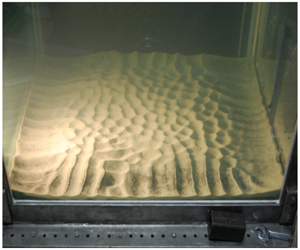
In our experiments, we observe the development of bedforms. Ripples are typically associated with mean flows or orbital motions, and have been observed and explored in a variety of field and experimental studies (Traykovski et al. Reference Traykovski, Hay, Irish and Lynch1999; Rodriguez-Abudo, Foster & Henriquez Reference Rodriguez-Abudo, Foster and Henriquez2013). Despite previous literature on ripple formation and migration in wave-driven flows, we observe them in the absence of such driving forces and correlate the spacing of the ripples with the integral length scale of the turbulence.
2 Experimental facility
2.1 Apparatus
The facility used to conduct the experimental study is housed in the DeFrees Hydraulics Laboratory at Cornell University. The apparatus consists of a 100.0 cm tall water tank with an  $80.0~\text{cm}\times 80.0~\text{cm}$ horizontal cross-sectional area; it is described in detail in Johnson & Cowen (Reference Johnson and Cowen2018). The base of the tank is filled with commercial Everlast play sand to a depth of 8 cm, which is sufficiently deep that the exact position of the impermeable facility boundary is unimportant. All of the sand is initially shaken through a no. 30 sieve with 600 μm openings to eliminate stones and debris, and it is frequently washed to remove fines. The sand is narrowly graded with a median diameter,
 $D_{50}$, of 260 μm. The distribution of grain sizes is such that
 $(D_{84}-D_{16})/2=123.5~\unicode[STIX]{x03BC}\text{m}$ and
 $(\unicode[STIX]{x1D6F7}_{84}-\unicode[STIX]{x1D6F7}_{16})/4+(\unicode[STIX]{x1D6F7}_{95}-\unicode[STIX]{x1D6F7}_{5})/6.6=0.7$, where
 $\unicode[STIX]{x1D6F7}=\log _{2}(d)$ and
 $d$ is measured in mm, suggesting moderately well sorted sand.
Prior to experiments, the sand bed is raked and flattened at the sediment–water interface to diminish prominent peaks, ripples and scour holes that develop during previous tests or experimental set-up procedures. Although the surface of the sediment bed is often not perfectly flat, imperfections in the initial state of less than 1 cm in height tend to disappear quickly after the inception of turbulence generation.
Two different downward facing RASJAs are suspended above the facility, as shown in figure 2. One RASJA is an 8 × 8 array of 2.19 cm diameter synthetic jets (12 V 2.1 A Rule 360 g.p.h. bilge pumps) with centre-to-centre spacing,  $J$, of 10.0 cm arranged on a square grid that obeys reflective symmetry at the sidewalls. The jet Reynolds number of each jet is
 $Re_{jet}=22\,000$ at
 $20\,^{\circ }\text{C}$ water. The 8 × 8 RASJA is mounted a height
 $H=71~\text{cm}$ above the top of the sediment bed, thus, the ratio
 $H/J$ is 7.1. The 16 × 16 RASJA consists of 256 8.0 mm diameter 12 V 2.8 A Rule il200 submersible inline pumps with spacing
 $J=5.0~\text{cm}$ and
 $Re_{jet}=28\,000$. The jet orifice plane is 65.0 cm above the sand bed with
 $H/J=13$.
Turbulence tank design shown with partial 8 × 8 RASJA (left) and partial 16 × 16 RASJA (right).

As described in Variano & Cowen (Reference Variano and Cowen2008), the jet on–off states are determined via a ‘sunbathing’ algorithm to produce optimal turbulent kinetic energy without inducing secondary mean flows or recirculations. The algorithm is controlled in Mathworks MATLAB using an Arduino Mega 2560 microcontroller to determine individual jet on–off states on a 10 Hz update frequency. The sunbathing algorithm randomly selects instantaneous on-times given user-input parameters  $T_{on}$ and
 $\unicode[STIX]{x1D6F7}_{on}$, the mean on-time of each jet and the mean percentage of jet activity, respectively, as described in Johnson & Cowen (Reference Johnson and Cowen2018). As was observed in Johnson (Reference Johnson2016),
 $\unicode[STIX]{x1D6F7}_{on}$ does not have a significant influence on the r.m.s. velocity or turbulent kinetic energy, and so a single percentage of active jets is selected for each of the RASJAs. With the 8 × 8 RASJA, a majority of the tests presented are from a selected
 $\unicode[STIX]{x1D6F7}_{on}$ of 6.25 %, and several tests were performed at
 $\unicode[STIX]{x1D6F7}_{on}$ of 12.5 %. With the 16 × 16 RASJA,
 $\unicode[STIX]{x1D6F7}_{on}=3.1\,\%$. Note that all jets run during a 30 min test, even with low values of
 $\unicode[STIX]{x1D6F7}_{on}$. To control turbulence levels, the mean on-times are varied such that
 $T_{on}=3$, 4, 6, 8 s for the 8 × 8 RASJA, and
 $T_{on}=0.8$, 1.0, 1.2, 1.4, 1.6 s with the 16 × 16 RASJA.
The coordinate system is shown in figure 2, with  $z=0$ at the top of the bed increasing upwards to
 $H$, the height of the jet orifices relative to the bed. At the lateral centre of the facility,
 $x=0$ and
 $y=0$, each orthogonal to the sidewalls and following the right-hand rule. Velocity components
 $U$,
 $V$ and
 $W$ follow the
 $x$-,
 $y$- and
 $z$-directions, respectively.
In random jet array driven facilities, a ratio  $H/J>6$ is required to ensure full mixing of the jets (Variano & Cowen Reference Variano and Cowen2008; Perez-Alvarado et al. Reference Perez-Alvarado, Mydlarski and Gaskin2016). Prior to achieving a distance from the jets equal to six times the jet spacing, or roughly
 $H-6J<z<H$, the jets are still merging and the flow is dominated by instantaneous jet activity driving distinct upward and downward flows. As determined in Johnson & Cowen (Reference Johnson and Cowen2018), the development of various flow characteristics is as follows. With the 8 × 8 RASJA, immediately beneath the jet merging region, the flow is fully mixed into horizontally homogeneous nearly isotropic turbulence and r.m.s. velocities remain relatively constant. In this region, the ratio of bed-normal to bed-parallel r.m.s. velocities is 1.3, consistent with measurements reported from the same facility by Johnson & Cowen (Reference Johnson and Cowen2018) and Variano & Cowen (Reference Variano and Cowen2008), along with similarly designed turbulence facilities (Hopfinger & Toly Reference Hopfinger and Toly1976; McDougall Reference McDougall1979). The lower bound of the mixed region is observed at
 $z=1.5{\mathcal{L}}_{L}$, where
 ${\mathcal{L}}_{L}$ signifies the longitudinal integral length scale, to be explored further in § 3. With the 16 × 16 RASJA, which is mounted non-dimensionally further from the bed, there is a decay region between the jet merging region and the mixed region, where r.m.s. velocities decay with distance from the jet array.
The flow beneath the mixed region transitions towards the region of flow influenced by the bottom boundary. In the bed-influenced region, there is a source region that is observed for  $0.15<z/{\mathcal{L}}_{L}<0.5$. The source region is defined by Hunt & Graham (Reference Hunt and Graham1978) as having significant intercomponent energy transfer, and it is here that we see evidence for dynamic turbulent splats (Perot & Moin Reference Perot and Moin1995a). Below
 $z/{\mathcal{L}}=0.15$ is the buffer region where r.m.s. velocities fall from their peak value towards zero at the bed. The buffer region in our experiments qualitatively compares well to the viscous region presented by Hunt & Graham (Reference Hunt and Graham1978), though it is clearly thicker than one would expect a true viscous region to extend. Beneath the buffer region, the viscous boundary layer thickness
 $\unicode[STIX]{x1D6FF}_{\unicode[STIX]{x1D708}}$ is calculated as 2.4 mm with the 8 × 8 RASJA and 1.1 mm with the 16 × 16 RASJA.
2.2 Measurement techniques
2.2.1 Particle image velocimetry
Spatio-temporal velocity measurements are made using particle image velocimetry (PIV) in the lateral centre of the tank in the  $x{-}z$ plane at and above the sediment bed. Two components of velocity,
 $U$ and
 $W$, are measured. Data are recorded at a sampling frequency of 1 Hz to collect uncorrelated samples, given estimates of the integral time scale of the turbulence of approximately 1.17 s and 0.67 s when using the 8 × 8 and 16 × 16 RASJAs, respectively (Johnson & Cowen Reference Johnson and Cowen2018). Images of 2056 by 2060 pixel resolution are collected using an Imperx Bobcat IGV-2020 camera. Illumination is provided by scanning a 3 W l.4 mm diameter Argon Ion beam (Coherent Innova 90 laser) across the field of view (FOV) from top to bottom. Scans are completed within 3.5 ms, and the time between images within a PIV image pair,
 $\unicode[STIX]{x0394}t$, is 8 ms. Additional details about the timing and mechanisms of PIV data collection are presented in Johnson & Cowen (Reference Johnson and Cowen2018). Although the jet array may be running for several hours before and/or after tests, PIV data are collected over 30 min periods, which is long enough for statistics to converge sufficiently (Variano & Cowen Reference Variano and Cowen2008) but not long enough for significant changes in sediment bedforms at the base of the facility.
For PIV measurements, the flow is seeded with Arkema Group ORGASOL (R) 2002 ES 3 Nat 3 Polyamide 12 nylon particles, which serve as passive tracers with Stokes number consistently less than 0.001. By contrast, the Stokes number for sand is equal to 1 at  $D=200~\unicode[STIX]{x03BC}\text{m}$. In the present experiments,
 $D_{50}=260~\unicode[STIX]{x03BC}\text{m}$, and so with Stokes numbers of order 1, the sand grains are not truly passive tracers for PIV measurements. However, sediment suspension is relatively infrequent, as described in § 5, and the analysis of PIV images with clearly suspended sand grains does not appear to produce different results from images absent suspension. This is in large part due to the results of testing via an artificial neural network, similar to that developed by van Maanen et al. (Reference van Maanen, Coco, Bryan and Ruessink2010), which yielded no obvious correlation between measured velocity and presence of suspended grains. Thus the inertia of suspended sediments is not expected to significantly alter the measured fluid velocity relative to the densely seeded ORGASOL tracer particles. Although we describe experiments with sediment suspension, the suspension events occur throughout the facility and are relatively infrequent in the PIV images themselves. For images in which suspended sediment is observed, sediment grains are treated as passive tracers.
Before images can be interrogated to identify particle displacements, the location of the bed must be properly identified. Above a flat plate, this is relatively straightforward, as the bed is uniformly illuminated across the width of the FOV. By computing a profile of average image intensity, we mark the base of the flow as being located one pixel above the uppermost location of peak image intensity. The bottom of the lowest subwindow is located at that pixel.
At a sand bed, this procedure is more complex. Because the bed is not uniform in  $x$, we create a mask, which is a spatial array of zeros and ones, to apply to each image. At pixel locations at and below the surface of the bed, determined on a column-wise basis (i.e.
 $x$-direction), the mask contains zeros, while pixels located above the bed are denoted by ones in the mask matrix. Once the mask is generated, it is simply multiplied by the original image so that only regions above the bed are kept for image interrogation.
To identify the location of the bed and create the mask, the data are first divided into 30 one minute increments. Computing masks instantaneously is troublesome as the mask-identifying algorithm can be confused by exceedingly bright tracer particles. On the other hand, the bed does not change positions substantially for several minutes so the one minute increment is a suitable compromise. A minimum background image is generated for each minute of data (60 image pairs) by finding the minimum value at each pixel within the image set (Cowen & Monismith Reference Cowen and Monismith1997). This effectively removes brightly illuminated tracer particles, so only the illuminated bed remains. The images are scanned for the uppermost pixel with an intensity of 4095, the maximum obtainable value with our 12-bit camera, and a reliable artefact of the bed surface. Because shadows cast by ripples on the sediment bed can prevent the entire bed from being fully illuminated, gaps in the mask are filled in via linear interpolation.
Once the images are pre-processed to handle sediment bed effects, background noise introduced by uniform ambient light is removed, as in Cowen & Monismith (Reference Cowen and Monismith1997), such that a temporal minimum background image across all images is computed, again in a pixel-by-pixel manner, and separating all first and second images within each pair due to variations in illumination. These background images are subtracted from all corresponding masked raw images. The images are then interrogated in 64 × 64 pixel subwindows with 50 % overlap using a second-order accurate in space and spectral correlation peak interpolation-based sub-pixel accurate PIV algorithm developed by Liao & Cowen (Reference Liao and Cowen2005) and based on Cowen & Monismith (Reference Cowen and Monismith1997). The resulting vectors from the coarse 64 × 64 pixel pass are then smoothed according to the median of valid vectors within a 3 × 3 array of neighbouring subwindows and interpolated onto a more refined grid for interrogation via 32 × 32 pixel subwindows with 50 % overlap. This final interrogation results in a 1.76 mm spatial resolution.
During PIV interrogation, there exist subwindows along the bed for which only part of the image remains for analysis (i.e. consists of ones in the original mask) and the remaining portion falls beneath the bed. If more than  $2/3$ of the pixels in a given subwindow are originally unmasked, then the subwindow is deemed to be sufficiently above the bed and the velocity vector for that subwindow remains valid. If fewer than the set threshold are originally ones, then the vector is flagged as an unreliable data point to be removed. This impacts the decision of where
 $z$ is equal to zero, as bed morphology necessarily causes variability in how many valid data points remained as a function of lateral position across the FOV. There are, perhaps surprisingly, no apparent signatures of flow dependence on bed morphology, and horizontal homogeneity remains intact above the rippled bed. We take
 $z=0$ at the lowest point in the FOV for which at least half of the subwindows were utilized.
Once analysis and the masking procedures are complete, several filters are applied to remove unconverged or erroneously determined velocity vectors. Once unconverged vectors are removed, an adaptive Gaussian filter (Cowen & Monismith Reference Cowen and Monismith1997) removes spurious vectors that exceed what is expected from the statistics of a Gaussian distribution of turbulent velocities. A spatial local median filter (Westerweel Reference Westerweel1994; Cowen & Monismith Reference Cowen and Monismith1997) then removes data exceeding a threshold relative to the nearest neighbour local median. As described in Johnson (Reference Johnson2016), spatial interpolation is used to fill in removed data only when spatial spectra (or statistics based upon spatial spectra) requiring a continuous dataset are computed; otherwise filtered uninterpolated data are used.
Reynolds decomposition is used to consider mean and fluctuating velocities as  $U(x,y,z,t)=\langle U(x,y,z)\rangle +u(x,y,z,t)$ and likewise for
 $W$. The angle brackets denote a temporal average and lower case letters represent fluctuations. According to 3-component velocity data in Johnson (Reference Johnson2016), the flow is radially symmetric about the
 $z$ axis. Thus we only report statistics along the
 $x{-}z$ plane and are able to invoke radial symmetry and continuity to statistically address the out-of-plane dynamics. Lateral variations across the 20 cm FOV are sufficiently small to invoke horizontal homogeneity. However, all computations are made prior to any temporal or spatial averaging, and all resulting profiles presented herein have been averaged both temporally and horizontally. An overbar denotes averages that include time and space (i.e. the horizontal average of
 $\langle U\rangle$ is
 $\overline{U}$).
We use the bootstrap method (Efron & Tibshirani Reference Efron and Tibshirani1993) to construct 95 % confidence intervals of the turbulence statistics to compute uncertainty bounds. With our assumptions of convergence and horizontal homogeneity, the bootstrap analyses presented typically utilize between 1800 and 225 000 data points, resampled 1000 times, with replacement, to generate ordered random statistics. The 95 % confidence interval is determined by the 2.5 percentile and 97.5 percentile statistics.
2.2.2 Time-lapsed photography
Ripple evolution observed at initial state, 15 min, 30 min, 1 h, 2 h, 4 h, 8 h and 12 h (a–h) into turbulence generation above an initially flat sediment bed.  $T_{on}=3~\text{s}$,
 $\unicode[STIX]{x1D6F7}_{on}=12.5\,\%$, 8 × 8 RASJA.

In order to monitor the evolution of large bedforms (i.e. ripples spanning 2–6 cm from crest to crest), we used time-lapsed photography. A single Nikon D40 camera was mounted beside the tank to capture still photos of the bed, with additional spotlights mounted normal to the tank to provide contrast over the ripple field. The camera was controlled using the application Sofortbild. Images were captured in set time increments (ranging from 1 min to 10 min) over periods of up to 24 h. A selection of these images is shown in figure 3. In addition to showing the temporal evolution of large-scale bed morphology, these images were used to measure the crest-to-crest ripple spacing at the conclusion of each experiment. More details are presented on ripple spacing in § 6.
3 Statistical analysis of turbulence metrics
Using PIV data, we explore the boundary layer that develops over both flat and rippled sand beds under nearly isotropic forcing from above. As mean flows are minimized in this facility for the RASJA operating conditions selected, fluctuating components of velocity are critical to understanding the energetics of the flow (Perot & Moin Reference Perot and Moin1995a; McCorquodale & Munro Reference McCorquodale and Munro2018). In experiments with the 8 × 8 RASJA, sediment suspension levels are consistently low, with visible suspension events occurring on order once per minute anywhere on the sediment bed. This is termed a mildly suspending bed. As can be seen in figure 3, the centre of the bed remained relatively flat for the first 2 h, despite ripples and small central dimples forming around the periphery. PIV experiments above a flat sediment bed were performed within one hour of turning the jets on to ensure negligible bedform development; for PIV experiments above a rippled sediment bed, the RASJA was run until the bed achieved a quasi-equilibrium ripple state, as described further in § 6. In experiments with the 16 × 16 RASJA, ripple development occurred within minutes of turning on the RASJA, and so a flat non-rippled sediment bed case was not available for comparison and only a rippled bed is considered. Interestingly, there were more frequent suspension events in experiments with the 16 × 16 RASJA, occurring on order once per 5–10 s. Thus, this rippled bed is considered to be moderately suspending. Suspension is detailed more thoroughly in § 5. Resulting boundary layer profiles above the three sediment conditions described (i.e. flat mildly suspending sediment, rippled mildly suspending sediment, rippled moderately suspending sediment) are also compared to the boundary layer profiles above a flat impermeable boundary explored in Johnson & Cowen (Reference Johnson and Cowen2018).
3.1 Mean velocities and turbulent velocity fluctuations
RASJA-driven facilities are advantageous in design as mean velocities and secondary mean flows can be minimized relative to turbulent velocity fluctuations. There is a weak mean flow in the centre of the tank with a return flow along the walls, as in Variano & Cowen (Reference Variano and Cowen2008) and Johnson & Cowen (Reference Johnson and Cowen2018). Mean horizontal velocities are of the order  $1~\text{mm}~\text{s}^{-1}$. Mean vertical velocities are greater in magnitude, varying from 1 to
 $8~\text{mm}~\text{s}^{-1}$, as shown in table 1. Note that the 8 × 8 RASJA has a downward central flow in all cases with the exception of a very weak upward central flow in the case of the
 $T_{on}=4~\text{s}$ flat sediment bed case, whereas the 16 × 16 RASJA has an upward central flow for all flows above a sediment bed.
Mean vertical velocities and secondary mean flow strengths in the mixed region.  $\unicode[STIX]{x1D6F7}_{on}=6.25\,\%$ for 8 × 8 RASJA;
 $\unicode[STIX]{x1D6F7}_{on}=3.1\,\%$ for 16 × 16 RASJA.

The r.m.s. velocities are computed as  $u^{\prime }=\sqrt{\langle u^{2}\rangle }$ and
 $w^{\prime }=\sqrt{\langle w^{2}\rangle }$. These provide a measure of the turbulence intensity in the bed-parallel and bed-normal directions, respectively. Note that, while turbulence intensity traditionally describes r.m.s. velocity normalized by the mean velocity, this quantity would be meaningless in a facility with negligible mean flow and thus dimensional quantities are used to represent turbulence intensity. We can compute a mean flow strength parameter,
 $M^{\ast }$ as a measure of the mean kinetic energy,
 $\langle U\rangle ^{2}+{\textstyle \frac{1}{2}}\langle W\rangle ^{2}$, relative to the turbulent kinetic energy,
 $k=\frac{1}{2}(2u^{\prime 2}+w^{\prime 2})$, computed by invoking radial symmetry. Across all experimental cases considered above a sediment bed, the maximum value of
 $M^{\ast }$ is 3 %, with several cases less than 1 %. With Variano & Cowen (Reference Variano and Cowen2008) determining secondary mean flows to negligibly affect gas transfer velocity at a free surface when
 $M^{\ast }<5\,\%$, we have confirmation that mean flows appear to be negligible in the present facility; however, we will revisit this assumption later in this section.
Focusing on the mixed and bed-influenced regions, we consider profiles of  $u^{\prime }$ and
 $w^{\prime }$ for the various bed conditions explored. Figure 4 shows resulting profiles computed from experiments with the 8 × 8 RASJA, with present data for a flat sediment bed and a rippled sediment bed, both with negligible contributions of suspension, in comparison with the flat solid bed results presented in Johnson & Cowen (Reference Johnson and Cowen2018). All profiles clearly show evidence of the kinematic boundary condition, in which bed-normal turbulent velocity fluctuations decay towards the bed whereas bed-parallel fluctuations increase, before both
 $u^{\prime }$ and
 $w^{\prime }$ decay towards zero at the bed itself. This intercomponent energy transfer is the strongest above the flat solid boundary, as the bed is fully impermeable, immobile and smooth. In the case of the flat sediment boundary, there is no noticeable change in
 $u^{\prime }$ as compared to the flat solid boundary. However, lower values of
 $w^{\prime }$ are observed above a flat sediment bed. We attribute this to the hydraulic conductivity of the sediment bed that allows weak penetration from bed-normal flows, consistent with the work of Schmeeckle (Reference Schmeeckle2015) and Voermans, Ghisalberti & Ivey (Reference Voermans, Ghisalberti and Ivey2018), among others. Similarly, we observe a slight decrease in the turbulent kinetic energy throughout the water column, as shown in figure 5, for a flat mildly suspending sediment bed compared to a flat solid bed. In the mixed region of the flow, this reduction amounts to approximately 5 % throughout the mixed region of the flow in the case shown. The experiments under these conditions have weak downward central flows, perhaps exhibiting behaviour of a suction boundary layer (Dutton Reference Dutton1958; Tennekes Reference Tennekes1965). Although a suction boundary layer is not possible through an impermeable solid plate, it is possible through a porous sediment bed. In measurements by Favre, Dumas & Verollet (Reference Favre, Dumas and Verollet1961), it was shown that r.m.s. velocities are reduced in the presence of suction. Indeed, in the present experiments, turbulence is reduced in these cases as evidenced in figures 4 and 5, with the downward flow thinning the boundary layer or sucking it towards the bed.
Profiles of  $u^{\prime }$ (black) and
 $w^{\prime }$ (grey) above solid impermeable (solid line), flat sediment (dash-dotted line) and rippled sediment (dotted line) mildly suspending boundaries.
 $\unicode[STIX]{x1D6F7}_{on}=6.25\,\%$,
 $T_{on}=4~\text{s}$, 8 × 8 RASJA.

Profiles of  $k$ above solid impermeable (solid line), flat sediment (dash-dotted line) and rippled sediment (dotted line) mildly suspending boundaries.
 $\unicode[STIX]{x1D6F7}_{on}=6.25\,\%$,
 $T_{on}=4~\text{s}$, 8 × 8 RASJA.

Examining profiles of r.m.s. velocities and turbulent kinetic energy above a rippled sediment bed with mild sediment suspension presented in figures 4 and 5, there is a decrease in the strength of the horizontal turbulent velocity fluctuations throughout the entire water column compared to the flat bed case as well as in the vertical turbulent velocity fluctuations above  $z=2~\text{cm}$ for both the flat bed and rippled porous bed cases. While it is tempting to deduce increased drag resulting from the bedforms could be the cause, we see the opposite in the 16 × 16 RASJA experiments (discussed below). The magnitude of the vertical turbulent velocity fluctuations are reduced in the flat sediment bed case relative to the impermeable flat glass bed case. In the rippled sediment bed case,
 $w^{\prime }$ is even further reduced as compared to the flat sediment case, for a mildly suspending bed. This suggests to us that the porosity of the permeable bed is playing an important role, which we will discuss further after exploring the 16 × 16 RASJA results. The decreases in both
 $u^{\prime }$ and
 $w^{\prime }$ lead to a reduction in
 $k$. Results are summarized in table 2.
Turbulent (r.m.s.) velocities and turbulent kinetic energy in the mixed region.  $\unicode[STIX]{x1D6F7}_{on}=6.25\,\%$. 8 × 8 RASJA.

To explore whether the development of bedforms affects the lateral homogeneity of the flow, dispersive stresses have been computed in addition to Reynolds stresses. As in King, Tinoco & Cowen (Reference King, Tinoco and Cowen2012), dispersive stress is defined as  $\unicode[STIX]{x1D70C}\overline{\langle u\rangle ^{\prime \prime }\langle w\rangle ^{\prime \prime }}$, where
 $\langle u\rangle ^{\prime \prime }=\langle u\rangle -\overline{\langle u\rangle }$ and similarly for
 $\langle w\rangle ^{\prime \prime }$. In computing the dispersive stress, no lateral variation was found. The magnitude of Reynolds stress
 $\unicode[STIX]{x1D70C}\langle uw\rangle$ was found to be less than 2 % of
 $k$. Dispersive stress was found to be less than 10 % of the Reynolds stress, and thus is negligible as expected in homogeneous turbulence.
In experiments with the 16 × 16 RASJA, in which sediment suspension is more prevalent and there is no stable flat bed sediment case, there are significant increases observed in  $u^{\prime }$,
 $w^{\prime }$ and
 $k$ above a sediment bed as compared to the solid glass bed, as shown in figures 6 and 7 and table 3. Again, this influences both the mixed region and boundary layer. This is contrary to the trends observed in experiments with the 8 × 8 RASJA that saw a decay in the energy above a sediment bed as compared to the solid glass bed. Recall also that a downward central mean flow exists with the 8 × 8 RASJA, whereas the 16 × 16 RASJA has an upward central flow. The shape between the profiles computed above solid and sediment beds is noticeably different as well, with less pronounced intercomponent energy transfer occurring over the sediment bed, as is evident in particular in the profiles of
 $u^{\prime }$ and
 $k$. The increase in
 $u^{\prime }$ and
 $k$ in the source layer, where we observe the strongest evidence of intercomponent energy transfer, is more gradual and lower in relative magnitude over sediment than above the solid glass boundary. This bump in energy very near the bed is likely due to pressure fluctuations, as in Johnson & Cowen (Reference Johnson and Cowen2018), and it will be further discussed in § 3.2.4.
Profiles of  $u^{\prime }$ (black) and
 $w^{\prime }$ (grey) above solid impermeable (solid line) and rippled sediment (dashed line) moderately suspending boundaries.
 $\unicode[STIX]{x1D6F7}_{on}=3.1\,\%$,
 $T_{on}=0.8~\text{s}$, 16 × 16 RASJA.

Profiles of  $k$ above solid impermeable (solid line) and rippled sediment (dashed line) moderately suspending boundaries.
 $\unicode[STIX]{x1D6F7}_{on}=3.1\,\%$,
 $T_{on}=0.8~\text{s}$, 16 × 16 RASJA.

Turbulent (r.m.s.) velocities and turbulent kinetic energy in the mixed region.  $\unicode[STIX]{x1D6F7}_{on}=3.1\,\%$. 16 × 16 RASJA.

As opposed to the 8 × 8 case, we now see a strong enhancement of  $u^{\prime }$,
 $w^{\prime }$ and hence
 $k$ throughout the measurement region relative to the impermeable glass bed case. We investigated the probability density functions (PDF) for the two flows at different elevations above the bed, finding both cases collapse well on each other as shown in figure 8.
Probability density functions of  $u^{\prime }$ (a) and
 $w^{\prime }$ (b) at
 $z=0.17~\text{cm}$ above the bed: × denotes glass; circle denotes sand; solid line denotes normal distribution.
 $\unicode[STIX]{x1D6F7}_{on}=3.1\,\%$,
 $T_{on}=0.8~\text{s}$, 16 × 16 RASJA.

One-sided spatial spectra  $G_{uu}$ (a) and
 $G_{ww}$ (b) above a moderately suspending sediment and impermeable glass boundary. Distance ranges from
 $z=1.2$ to
 $z=11.4~\text{cm}$. Black lines represent glass bed, grey lines represent sediment bed, dotted line
 $-5/3$ slope.
 $\unicode[STIX]{x1D6F7}_{on}=3.1\,\%$,
 $T_{on}=0.8~\text{s}$, 16 × 16 RASJA.

One-sided spatial spectra  $G_{uu}$ (a) and
 $G_{ww}$ (b) above a moderately suspending sediment and impermeable glass boundary. Distance ranges from
 $z=1.2$ to
 $z=11.4~\text{cm}$. Black lines represent glass bed, grey lines represent sediment bed, dashed line
 $-5/3$ slope.
 $\unicode[STIX]{x1D6F7}_{on}=3.1\,\%$,
 $T_{on}=0.8~\text{s}$, 16 × 16 RASJA.

We next consider one-sided spatial spectra at multiple elevations, both dimensional (figure 9) and non-dimensional (figure 10). The spectra are computed as the Fourier transform of the autocorrelation of the velocity, with  $G_{uu}$ computed from the bed-parallel velocity
 $U$ and
 $G_{ww}$ from the bed-normal velocity
 $W$. Looking at figure 9, clearly the energy starting around wavenumber
 $\unicode[STIX]{x1D705}=2~\text{rad}~\text{cm}^{-1}$ is greater for the moderately suspending sediment bed relative to the impermeable glass bed, corresponding to length scales less than approximately 3 cm. Figure 10 shows spectra
 $G_{uu}$ and
 $G_{ww}$ non-dimensionalized using r.m.s. velocities and integral scales
 ${\mathcal{L}}_{L}$ and
 ${\mathcal{L}}_{T}$, to be discussed further in § 3.3. The non-dimensionalized spectra demonstrate good collapse when scaled by the respective integral length scales, and the energy at higher wavenumbers in the suspending sediment bed case remains apparent.
As mentioned previously, experiments performed with the 16 × 16 RASJA have a weak upward central flow. Indeed, the profiles presented in figures 6 and 7 are reminiscent of a blowing boundary layer (Mickley & Davis Reference Mickley and Davis1957). In particular, the significant increase in r.m.s. velocities and  $k$, along with the smoothing of features with distance from the bed draw similarity to results shown by Ferro (Reference Ferro2017) of a transpiring turbulent boundary. Andersen, Kays & Moffat (Reference Andersen, Kays and Moffat1972) and Kornilov (Reference Kornilov2015) observed a magnification in
 $u^{\prime }$ and
 $w^{\prime }$. The boundary layer is pushed farther from the wall, moving the turbulent structures away from the kinematic boundary condition. It is noteworthy that blowing does not only affect near-bed energetics, but affects turbulent velocity fluctuations most significantly in the outer part of the boundary layer (Ferro Reference Ferro2017), consistent with our present observations.
3.2 Turbulent kinetic energy balance
In the full turbulent kinetic energy budget,
 $$\begin{eqnarray}\frac{\unicode[STIX]{x2202}k}{\unicode[STIX]{x2202}t}+\langle U_{j}\rangle \frac{\unicode[STIX]{x2202}k}{\unicode[STIX]{x2202}x_{j}}=-\frac{1}{\unicode[STIX]{x1D70C}_{0}}\frac{\unicode[STIX]{x2202}\langle u_{i}p\rangle }{\unicode[STIX]{x2202}x_{i}}-\frac{1}{2}\frac{\unicode[STIX]{x2202}\langle u_{j}u_{j}u_{i}\rangle }{\unicode[STIX]{x2202}x_{i}}+\unicode[STIX]{x1D708}\frac{\unicode[STIX]{x2202}^{2}k}{\unicode[STIX]{x2202}x_{j}^{2}}-\langle u_{i}u_{j}\rangle \frac{\unicode[STIX]{x2202}\langle U_{i}\rangle }{\unicode[STIX]{x2202}x_{j}}-\unicode[STIX]{x1D708}\left\langle \frac{\unicode[STIX]{x2202}u_{i}\unicode[STIX]{x2202}u_{i}}{\unicode[STIX]{x2202}x_{j}\unicode[STIX]{x2202}x_{j}}\right\rangle +\langle w^{\prime }b^{\prime }\rangle\end{eqnarray}$$
several terms are found to be negligible in horizontally homogeneous nearly isotropic turbulence with constant forcing, including  $\unicode[STIX]{x2202}k/\unicode[STIX]{x2202}t$,
 $\langle U_{j}\rangle (\unicode[STIX]{x2202}k/\unicode[STIX]{x2202}x_{j})$ and
 $\unicode[STIX]{x1D708}(\unicode[STIX]{x2202}^{2}k/\unicode[STIX]{x2202}x_{j}^{2})$, as in Johnson & Cowen (Reference Johnson and Cowen2018). Turbulent transport, production and dissipation, can be computed directly from PIV data. In general, buoyancy production
 $\langle w^{\prime }b^{\prime }\rangle$ should be considered with suspension occurring above a sediment bed, but in our case, where we have demonstrated the relatively low level of suspension, even in the 16 × 16 case, and found no evidence of statistical flow differences with sediment suspension present or absent, we can neglect this term.
In Johnson & Cowen (Reference Johnson and Cowen2018), the magnitude of pressure was calculated as the residual of dissipation, turbulent transport and production, as the only strictly non-zero terms remaining in the full turbulent kinetic energy balance. With a potential contribution from buoyancy, this could affect the magnitude of pressure. However, given our assumption of a negligible contribution of buoyancy given the relatively low frequency of suspension, the magnitude of pressure diffusion is estimated as
 $$\begin{eqnarray}-\frac{1}{\unicode[STIX]{x1D70C}_{0}}\frac{\unicode[STIX]{x2202}\langle u_{i}p\rangle }{\unicode[STIX]{x2202}x_{i}}=\frac{1}{2}\frac{\unicode[STIX]{x2202}\langle u_{j}u_{j}u_{i}\rangle }{\unicode[STIX]{x2202}x_{i}}+\langle u_{i}u_{j}\rangle \frac{\unicode[STIX]{x2202}\langle U_{i}\rangle }{\unicode[STIX]{x2202}x_{j}}+\unicode[STIX]{x1D708}\left\langle \frac{\unicode[STIX]{x2202}u_{i}\unicode[STIX]{x2202}u_{i}}{\unicode[STIX]{x2202}x_{j}\unicode[STIX]{x2202}x_{j}}\right\rangle .\end{eqnarray}$$
3.2.1 Dissipation
Invoking radial symmetry from earlier acoustic Doppler velocimetry measurements (Johnson Reference Johnson2016) and continuity (Cowen & Monismith Reference Cowen and Monismith1997; Doron et al. Reference Doron, Bertuccioli, Katz and Osborn2000), the dissipation rate can be computed directly as
 $$\begin{eqnarray}\displaystyle \unicode[STIX]{x1D716} & = & \displaystyle 2\unicode[STIX]{x1D708}\left[4\left\langle \left(\frac{\unicode[STIX]{x2202}u}{\unicode[STIX]{x2202}x}\right)^{2}\right\rangle +\left\langle \left(\frac{\unicode[STIX]{x2202}u}{\unicode[STIX]{x2202}z}\right)^{2}\right\rangle +\left\langle \left(\frac{\unicode[STIX]{x2202}w}{\unicode[STIX]{x2202}x}\right)^{2}\right\rangle +2\left\langle \left(\frac{\unicode[STIX]{x2202}w}{\unicode[STIX]{x2202}z}\right)^{2}\right\rangle \right.\nonumber\\ \displaystyle & & \displaystyle +\left.2\left\langle \left(\frac{\unicode[STIX]{x2202}u}{\unicode[STIX]{x2202}x}\frac{\unicode[STIX]{x2202}w}{\unicode[STIX]{x2202}z}\right)\right\rangle +2\left\langle \left(\frac{\unicode[STIX]{x2202}u}{\unicode[STIX]{x2202}z}\frac{\unicode[STIX]{x2202}w}{\unicode[STIX]{x2202}x}\right)\right\rangle \!\right]\end{eqnarray}$$
from two-dimensional PIV measurements. This calculation requires fine enough spatial resolution of PIV data to accurately measure instantaneous velocity gradients. Indeed, the spatial resolution is equal to  $8\unicode[STIX]{x1D702}$, meaning that we are able to compute 92 % of the total dissipation by computing dissipation directly from PIV measurements according to the integration of the universal spectrum (Pao Reference Pao1965; Cowen & Monismith Reference Cowen and Monismith1997). As in Johnson & Cowen (Reference Johnson and Cowen2018), this result is scaled up by a factor of 1.09 to account for this discrepancy between the spatial resolution of the present PIV measurements and the Kolmogorov length scale of the turbulence.
We compute dissipation profiles directly and find, when compared to the boundary layer above a flat solid bed, a mildly suspending sediment bed causes a reduction in the dissipation rate throughout the water column, which is consistent with the reduction in  $k$ for a mildly suspending sediment bed of the 8 × 8 RASJA. Despite the reduction in magnitude, the shape of the dissipation profile shows a similar structure to that observed above the solid boundary case in Johnson & Cowen (Reference Johnson and Cowen2018). Sediment transport is infrequent in these experiments. The mean downward flow reduces
 $k$ in the boundary layer and hence
 $\unicode[STIX]{x1D716}$ is lower as well. The difference in dissipation between the flat and rippled cases is inconclusive with regard to which causes the greatest reduction in dissipation, as is shown in figure 11 and summarized in table 4. There are instances in which the magnitude of dissipation is higher above a rippled sediment bed and other instances in which the dissipation is greater above a flat sediment bed; in either case, dissipation above a sediment bed with the 8 × 8 RASJA is similar whether rippled or flat, and both are less than the solid case by approximately 30 %, again consistent with a suction boundary layer.
Profiles of dissipation above solid impermeable (solid line), flat mildly suspending sediment (dash-dotted line) and rippled mildly suspending sediment (dotted line) boundaries. (a) Shows results for  $\unicode[STIX]{x1D6F7}_{on}=6.25\,\%$,
 $T_{on}=4~\text{s}$; (b) shows results for
 $\unicode[STIX]{x1D6F7}_{on}=6.25\,\%$,
 $T_{on}=8~\text{s}$. 8 × 8 RASJA.

Scales of turbulence in the mixed region, 8 × 8 RASJA.

For flow above the moderately suspending sediment bed of the  $16\times 16$ RASJA, shown in figure 12, there is a higher magnitude of
 $\unicode[STIX]{x1D716}$ for the rippled sediment boundary as compared to the solid bed, again, consistent with above results of r.m.s. velocities and turbulent kinetic energy. It is noteworthy that the slope of the decay of
 $\unicode[STIX]{x1D716}$ is less steep in the presence of suspending sediment, suggesting a better mixed, or more homogeneous, lower portion of the tank vertically. This is also consistent with the upward mean flow, or blowing boundary layer theory, with less prominent near-bed variation of the turbulence.
Dissipation profiles above solid impermeable (solid line) and moderately suspending sediment (dashed line) boundaries.  $\unicode[STIX]{x1D6F7}_{on}=3.1\,\%$,
 $T_{on}=0.8~\text{s}$, 16 × 16 RASJA.

With the change in  $\unicode[STIX]{x1D716}$ between the solid and rippled sediment cases under 16 × 16 forcing, the Kolmogorov time scale,
 $\unicode[STIX]{x1D70F}=(\unicode[STIX]{x1D708}/\unicode[STIX]{x1D716})^{1/2}$, and Kolmogorov length scale,
 $\unicode[STIX]{x1D702}\equiv (\unicode[STIX]{x1D708}^{3}/\unicode[STIX]{x1D716})^{1/4}$, where
 $\unicode[STIX]{x1D708}$ denotes the kinematic viscosity of water at 20 C, subsequently vary weakly with boundary condition. As a consequence of changing
 $\unicode[STIX]{x1D702}$, the Taylor microscale,
 $\unicode[STIX]{x1D706}_{g}=\sqrt{10}\unicode[STIX]{x1D702}^{2/3}{\mathcal{L}}^{1/3}$, and Taylor Reynolds number,
 $Re_{\unicode[STIX]{x1D706}}=(\frac{2}{3}k)\sqrt{15/\unicode[STIX]{x1D708}\unicode[STIX]{x1D716}}$, are also affected, as shown in tables 4–7. Interestingly, these lead to a change in the thickness of the viscous sublayer that develops above solid or sediment boundaries, which we approximate as
 $\unicode[STIX]{x1D6FF}_{\unicode[STIX]{x1D708}}\approx 2L_{L}Re_{L}^{-1/2}$, where
 $Re_{L}=Re^{\ast }=k^{2}/\unicode[STIX]{x1D716}\unicode[STIX]{x1D708}$ (Brumley & Jirka Reference Brumley and Jirka1987; Calmet & Magnaudet Reference Calmet and Magnaudet2003; Variano & Cowen Reference Variano and Cowen2008; Johnson & Cowen Reference Johnson and Cowen2018). Whereas
 $Re_{\unicode[STIX]{x1D706}}$ and
 $Re_{L}$ are affected by the change in the dissipation rate between boundary conditions, the grid Reynolds number,
 $Re_{G}=2((\sqrt{\frac{2}{3}k}{\mathcal{L}})/\unicode[STIX]{x1D708})$, used for comparison to GST experiments, is relatively unchanged.
Reynolds numbers in the mixed region, 8 × 8 RASJA.

Scales of turbulence, 16 × 16 RASJA.

Reynolds numbers in the mixed region, 16 × 16 RASJA.

3.2.2 Production
Production of turbulent kinetic energy is computed as
 $$\begin{eqnarray}{\mathcal{P}}=-\left[4\langle uu\rangle \frac{\unicode[STIX]{x2202}\langle U\rangle }{\unicode[STIX]{x2202}x}+2\langle uw\rangle \frac{\unicode[STIX]{x2202}\langle U\rangle }{\unicode[STIX]{x2202}z}+2\langle uw\rangle \frac{\unicode[STIX]{x2202}\langle W\rangle }{\unicode[STIX]{x2202}x}+\langle ww\rangle \frac{\unicode[STIX]{x2202}\langle W\rangle }{\unicode[STIX]{x2202}z}\right].\end{eqnarray}$$
In the turbulent kinetic energy budget of a boundary layer in channel flow, presented by Spalart (Reference Spalart1988), production and dissipation rates are shown to balance one another at the wall. Compared to the dissipation rate, in the present experiments the magnitude of production is less than approximately half the dissipation magnitude above a mildly suspending bed and approximately 10 % of the dissipation for a moderately suspending bed as in figure 14. However, in a mean shear free turbulent boundary layer above a flat solid bed, production, averaged in time, is found to be negligible due to weak mean velocity gradients (Johnson & Cowen Reference Johnson and Cowen2018). In experiments of turbulence absent mean shear above a sediment boundary, we observe a similar but not identical result; production of turbulent kinetic energy above a sediment bed is not strictly zero. In exploring the mean velocity gradients, shown in figure 13, and Reynolds stresses that comprise  ${\mathcal{P}}$,
 $\langle uw\rangle$,
 $\unicode[STIX]{x2202}\langle U\rangle /\unicode[STIX]{x2202}z$ and
 $\unicode[STIX]{x2202}\langle W\rangle /\unicode[STIX]{x2202}x$ are approximately equal to zero. As in the case of turbulence absent mean shear above a solid boundary,
 $\unicode[STIX]{x2202}\langle U\rangle /\unicode[STIX]{x2202}x$ being weakly non-zero is amplified by
 $\langle uu\rangle$ and contributes to non-zero
 ${\mathcal{P}}$ (Johnson Reference Johnson2016). Unlike in the solid boundary case,
 $\unicode[STIX]{x2202}\langle W\rangle /\unicode[STIX]{x2202}z$ is also non-zero in the present experiments, due to the hydraulic conductivity of the sediment bed. This ultimately increases the magnitude of
 ${\mathcal{P}}$, as seen in figure 14, though not enough to balance dissipation as in a channel flow.
Comparison of mean velocity gradient profiles  $\unicode[STIX]{x2202}\langle U\rangle /\unicode[STIX]{x2202}x$ (solid line);
 $\unicode[STIX]{x2202}\langle U\rangle /\unicode[STIX]{x2202}z$ (dash-dotted line);
 $\unicode[STIX]{x2202}\langle W\rangle /\unicode[STIX]{x2202}x$ (dashed line);
 $\unicode[STIX]{x2202}\langle W\rangle /\unicode[STIX]{x2202}z$ (dotted line) as measured above a moderately suspending sediment boundary. Four-point averages.
 $\unicode[STIX]{x1D6F7}_{on}=3.1\,\%$,
 $T_{on}=0.8~\text{s}$, 16 × 16 RASJA.

Dissipation (dashed), turbulent transport (dash-dotted), production (dotted) and estimated pressure diffusion (solid line). Values normalized by the average of  $\unicode[STIX]{x1D716}$ and
 ${\mathcal{L}}$ in the mixed region. Flat solid bed (a), flat mildly suspending sediment bed (b), rippled mildly suspending sediment bed (c).
 $T_{on}=4~\text{s}$,
 $\unicode[STIX]{x1D6F7}_{on}=6.25\,\%$, 8 × 8 RASJA.

3.2.3 Turbulent transport
The triple correlations, or turbulent transport, can be computed directly as
 $$\begin{eqnarray}T=-\frac{1}{2}\left[4\frac{\unicode[STIX]{x2202}\langle uuu\rangle }{\unicode[STIX]{x2202}x}+2\frac{\unicode[STIX]{x2202}\langle wwu\rangle }{\unicode[STIX]{x2202}x}+2\frac{\unicode[STIX]{x2202}\langle uuw\rangle }{\unicode[STIX]{x2202}z}+\frac{\unicode[STIX]{x2202}\langle www\rangle }{\unicode[STIX]{x2202}z}\right]\end{eqnarray}$$
from two-dimensional PIV measurements, invoking radial symmetry. Between the solid and sediment boundary, there is little difference in the resulting turbulent transport profiles, examples of which are shown in figure 14.
The magnitude of transport is comparable throughout the bulk of the measurement regions in the two facilities. The primary difference in boundary condition is within approximately 0.5 mm of the bed. Whereas the triple correlation clearly decays to zero at the solid bed, as expected with a no-slip boundary, this decay is not as clearly observed above a sediment bed above both flat and rippled conditions where hydraulic conductivity and sediment mobility affect the flow.
3.2.4 Pressure diffusion
In the absence of pressure measurements, the pressure diffusion term,  $P=(1/\unicode[STIX]{x1D70C}_{0})(\unicode[STIX]{x2202}\langle u_{i}p\rangle /\unicode[STIX]{x2202}x_{i})$, is calculated as the residual of the dissipation, production and turbulent transport, as in Johnson & Cowen (Reference Johnson and Cowen2018). Without precise measurements from pressure sensors or fully spatio-temporally resolved data, the pressure is computed with order of magnitude accuracy only. In the absence of advection or viscous diffusion, and with turbulent transport and production approximately equal to zero at the bed, the pressure diffusion term is significant to balance the dissipation rate. As no other mechanisms can be identified to generate energy in the temporally averaged turbulent kinetic energy balance, the hypothesis remains, as in Johnson & Cowen (Reference Johnson and Cowen2018), that regardless of bed condition among those explored in the present and preceding work (permeable, impermeable, flat, rippled, suspending, non-suspending) that pressure fluctuations generated by the impingement of strong velocity fluctuations with the boundary are capable of producing the energy presented in § 3.
In comparing the various bed conditions for experiments with the 8 × 8 RASJA, shown in figure 14, most notable is the slight increase in turbulent transport for  $z/{\mathcal{L}}<1.5$ with a sediment bed, which causes the magnitude of the pressure diffusion term to become negative above
 $z/{\mathcal{L}}>1.5$. By contrast, above a solid bed, transport is roughly zero everywhere. Above the rippled sediment bed, production appears not to decay to zero at the bed as well as above the flat beds, thus causing the magnitude of pressure to be weaker than in the flat cases.
3.3 Integral length scale
There are several length scales of interest in these experiments, including but not limited to: jet spacing, jet height, sediment diameter, ripple spacing, boundary layer thickness and fluid motion length scales such as the Kolmogorov, Taylor and integral length scales. It is important to explore relationships between imposed geometry, resultant fluid motion length scales and resultant sediment length scales in order to deduce relationships and correlations. One important scale of turbulent fluid motion is the integral length scale, which serves as a measure of the size of predominant eddies in the mixed region of the turbulent flow.
As in Johnson & Cowen (Reference Johnson and Cowen2018), we compute the longitudinal integral length scale  ${\mathcal{L}}_{L}$ using an exponential curve fit to the spatial longitudinal autocorrelation function,
 $$\begin{eqnarray}a_{11,1}(r)=\frac{\left\langle u\left(x_{c}-{\displaystyle \frac{r}{2}}\right)u\left(x_{c}+{\displaystyle \frac{r}{2}}\right)\right\rangle }{\left(\left\langle u\left(x_{c}-{\displaystyle \frac{r}{2}}\right)^{2}\right\rangle \left\langle u\left(x_{c}+{\displaystyle \frac{r}{2}}\right)^{2}\right\rangle \right)^{1/2}},\end{eqnarray}$$
such that  $r$ is the spatial separation along the horizontal axis, as in Variano & Cowen (Reference Variano and Cowen2008). We determine
 ${\mathcal{L}}_{L}$ using
 $a_{L}(r)=\text{e}^{-r/{\mathcal{L}}_{L}}$ as in Johnson & Cowen (Reference Johnson and Cowen2018), and we take the integral length scale,
 ${\mathcal{L}}$, of the turbulence to be equal to the longitudinal integral length scale in the mixed region. The transverse integral length scale,
 ${\mathcal{L}}_{T}$, is also computed according to methods developed in Johnson & Cowen (Reference Johnson and Cowen2018), to describe bed-normal eddy lengths. Above a solid bed, it was shown that the integral length scale increases with
 $T_{on}$ of the RASJA algorithm when using the 8 × 8 RASJA. This trend is observed above a flat sediment bed as well, when measured in the mixed region of the flow, as shown in table 8.
Integral length scale results in the mixed region above mildly suspending sediment bed.  $\unicode[STIX]{x1D6F7}_{on}=6.25\,\%$, 8 × 8 RASJA.

Above a rippled bed, this relationship is weakened, suggesting a feedback mechanism on the flow from the presence of ripples, consistent with our finding below that the ripple spacing scales with  ${\mathcal{L}}$. When using the 16 × 16 RASJA, differences in
 $T_{on}$ between experiments are too small to observe significant differences in
 ${\mathcal{L}}$, though there is a weak dependence of
 $T_{on}$ on
 ${\mathcal{L}}$, as shown in table 9. Additional details are presented in Johnson (Reference Johnson2016).
Integral length scale results in the mixed region above solid and moderately suspending sediment beds.  $\unicode[STIX]{x1D6F7}_{on}=3.1\,\%$, 16 × 16 RASJA.

4 Bed stress characterization
Characterizing the bed stress is non-trivial in a flow with negligible mean shear. Classic viscous shear stress
 $$\begin{eqnarray}\unicode[STIX]{x1D70F}_{v}=\unicode[STIX]{x1D707}\frac{\text{d}\overline{U}}{\text{d}z}\end{eqnarray}$$
does not accurately represent the bed shear in this type of flow, as  $\langle U\rangle$ and any spatial gradient thereof is nearly zero when averaged over time in this stationary flow. Furthermore, although there are strong instantaneous local shear events acting upon the boundary, we are unable to capture their magnitude in the true viscous boundary layer through our PIV measurements due to the interrogation resolution. Thus, we look to the Reynolds stress
 $$\begin{eqnarray}\unicode[STIX]{x1D70F}_{Re}=\unicode[STIX]{x1D70C}\langle uw\rangle .\end{eqnarray}$$
The magnitude of  $\unicode[STIX]{x1D70F}_{Re}$ at the edge of a shear-driven boundary layer is equivalent to
 $\unicode[STIX]{x1D70F}_{v}$ at
 $z=0$ at a hydraulically smooth boundary (Pope Reference Pope2000). Although the Reynolds stress is not a perfect substitute for viscous bed stress in the context of predicting sediment transport in response to instantaneous bursts (Heathershaw & Thorne Reference Heathershaw and Thorne1985; Nelson et al. Reference Nelson, Shreve, McLean and Drake1995), the magnitude of the Reynolds stress remains of interest in the general stress condition at the boundary. When computing Reynolds stresses over the duration of the experiment, we find a negligible contribution to stress when averaged over time due to homogeneity.
Both viscous and Reynolds stresses must be significant over short time scales, due to the sediment transport observed, and we explore a means to characterize events over short time periods. We consider production,  ${\mathcal{P}}=-\langle u_{i}u_{j}\rangle (\unicode[STIX]{x2202}\langle U_{i}\rangle /\unicode[STIX]{x2202}x_{j})$, which has contributions from both Reynolds stress components
 $\langle u_{i}u_{j}\rangle$ and mean velocity gradients
 $\unicode[STIX]{x2202}\langle U_{i}\rangle /\unicode[STIX]{x2202}x_{j}$. When averaged over 30 min,
 ${\mathcal{P}}$ is nearly zero, as discussed previously. Instantaneous fluctuations are not sufficient to mobilize sediment, as there must be some duration of an applied stress to achieve movement (Diplas et al. Reference Diplas, Dancey, Celik, Valyrakis, Greer and Akar2008). Over short time scales, however, of the order of seconds or tens of seconds, we observe considerably higher magnitudes of
 ${\mathcal{P}}$. To reveal this, we break the temporal record of PIV data into increments ranging from 3 s to 20 s. Production is computed based on the mean flow and velocity fluctuations within that period only. Thus, too small of a record results in negligible fluctuations, and too long of a record results in negligible mean velocities. Maximum values of production are attained for a period of 7 s, which is of the order of 10 integral time scales, for the trial in which
 $\unicode[STIX]{x1D6F7}_{on}=3.1\,\%$,
 $T_{on}=0.8~\text{s}$ with the 16 × 16 RASJA, for example, as shown in figure 15.
Maximum magnitude of production obtained with varying time intervals.  $\unicode[STIX]{x1D6F7}_{on}=3.1\,\%$,
 $T_{on}=0.8~\text{s}$, 16 × 16 RASJA.

Using the short time period over which production is maximized, we compute  $\unicode[STIX]{x1D70F}_{Re}$ at the edge of the boundary layer, where
 $k$ is maximized at the edge of the source region. In a shear-driven flow, there is a peak in
 $\unicode[STIX]{x1D70F}_{Re}$ at the edge of the viscous boundary layer from which we can approximate the magnitude of viscous shear, then
 $\unicode[STIX]{x1D70F}_{Re}$ decreases with distance from the bed. In experiments with negligible mean shear,
 $\unicode[STIX]{x1D70F}_{Re}$ does not peak, but instead continually increases with height. By constructing a histogram of the Reynolds stresses computed from short increments, as shown in figure 16, we can better understand the magnitude of instantaneous stress events and their associated friction velocities,
 $$\begin{eqnarray}u_{\ast }=\sqrt{\frac{|\unicode[STIX]{x1D70F}_{Re}|}{\unicode[STIX]{x1D70C}}},\end{eqnarray}$$
calculated from the magnitude of short-time Reynolds stresses in the histogram. As expected, the histogram of Reynolds stresses is centred about zero, which tells little about the high magnitude stress events that result in intermittent sediment motion and pick-up. Carrying out the computation using the median Reynolds stress would produce a negligible friction velocity. Instead, the tails of the histogram contain the information about the likelihood of an extreme instantaneous local event to mobilize sediment at the bed.
Histogram of  $\unicode[STIX]{x1D70F}_{Re}$ (at 7 s intervals) measured at
 $z=1~\text{cm}$.
 $\unicode[STIX]{x1D6F7}_{on}=6.25\,\%$,
 $T_{on}=4~\text{s}$, 8 × 8 RASJA.

Specifically, it is useful to consider what occurs at various percentiles of the Reynolds stress distribution. We compute the percentiles of the Reynolds stress distribution and calculate their associated friction velocities, as shown in table 10. While the distribution is roughly symmetric, it is not precisely centred upon zero with symmetric tails. To assign specific values that correspond to the value in a perfectly symmetric distribution in table 11, we compute the average of the matching percentiles on either side of the median. For example, to identify the values of friction velocity exceeded by the outermost 1 % of the data, we average the friction velocities found for the 0.5 and 99.5 percentiles.
Percentiles of Reynolds stress distribution and corresponding friction velocities.  $\unicode[STIX]{x1D6F7}_{on}=6.25\,\%$,
 $T_{on}=4~\text{s}$, 8 × 8 RASJA.

Lower bounds of tails of the friction velocity  $u_{\ast }$ (
 $\text{cm}~\text{s}^{-1}$) distribution for three RASJA settings.

Clearly, the friction velocities found in the tails of the Reynolds stress histogram over short time periods are significant in comparison to those centred about the median. From the van Rijn (Reference van Rijn1984) interpretation of the Shields curve, it is expected that a critical  $u_{\ast }$ of
 $1.3~\text{cm}~\text{s}^{-1}$ corresponds to incipient sediment motion for the sand used in our experiments. Indeed, our data show that this critical stress is exceeded in the outermost ranges of the histograms at the 25th and 75th percentiles in the case for which
 $\unicode[STIX]{x1D6F7}_{on}=6.25\,\%$ and
 $T_{on}=4~\text{s}$ with the 8 × 8 RASJA, for example. The likelihood of exceeding this stress in tests shown with the 16 × 16 RASJA is even higher, consistent with the increased observations of sediment transport to be discussed in the upcoming section.
5 Sediment suspension mechanisms
Two distinct phenomena are observed that result in sediment suspension from the bed in which sand grains are picked up and briefly entrained in the fluid flow above the bed. The first is vortical in nature, much like a dust devil (Sinclair Reference Sinclair1968) or whirlwind that spins about a predominantly vertical axis and travels laterally across the bed. Suspended vortices were observed to be highly three dimensional in nature, with sediment clouds rapidly changing orientation and concentration, as observed in Finn, Li & Apte (Reference Finn, Li and Apte2016). These structures are typically attached to the bed and are able to entrain additional sediment as they travel, due to the low pressure in the core of the vortex that encourages sediment pick-up. In experiments with the 8 × 8 RASJA, bed-attached vortices, an example of which is shown in figure 17(a), reach approximately 1–5 cm above the bed and are less than 2 cm in diameter according to visual estimates. In experiments with the 16 × 16 RASJA, these structures can grow significantly larger and entrain sand grains up to approximately 10 cm above the bed with diameters up to approximately 5 cm. On occasion, these large vortices can fill the entire FOV, with suspended sediment round at the top of the jets. This is consistent with figure 12, which showed increased vertical homogeneity in experiments with a moderately suspending sediment bed. These large vortices appear to be more short lived than their smaller and more common counterparts.
Images of sediment suspension generated bed-attached vortex (a) and turbulent splat (b).  $\unicode[STIX]{x1D6F7}_{on}=12.5\,\%$,
 $T_{on}=3~\text{s}$, 8 × 8 RASJA.

From visual observations, vortices appear more frequently over flat terrain rather than a rippled bed, though they can form anywhere. There appear to be no lasting effects on large-scale bed morphology as a result of vortices; small trails that form as sediment is entrained into the vortex or is deposited after falling out of suspension are quickly erased by other turbulent flow structures near the bed. Figure 18 shows a sample image in which two bed-attached vortices were present in the FOV. The high concentration of sand near the bed shows the cores of the vortices. The vortex on the left is contained within the bottom 1.5 cm above the bed, whereas the vortex on the right appears connected to a larger cloud of suspended sediment entrained above.
Image of sediment suspension generated via bed-attached vortices (a) and turbulent splat (b).  $\unicode[STIX]{x1D6F7}_{on}=3.1\,\%$,
 $T_{on}=1.6~\text{s}$, 16 × 16 RASJA.

The second suspension phenomenon is generated via turbulent splats, or the interaction of multiple adjacent splats into anti-splats (Perot & Moin Reference Perot and Moin1995a). Termed ‘permeable splat events’ by Schmeeckle (Reference Schmeeckle2015) and Leary & Schmeeckle (Reference Leary and Schmeeckle2017), suspension events from splats occur when flows approaching the bed turn radially outward along the bed from the central location of the splat, consistent with the intercomponent energy transitions observed in figures 4 and 6. These were observed as clusters of sediment grains being entrained in the flow only a few millimetres above the bed and radiating outwards, examples of which are shown in figures 17(b) and 18(b).
When multiple splats interacted, in that various strong instantaneous bed-parallel flows approached one another, sediment was ejected vertically upward from the bed. Vortices occasionally formed as a result of anti-splats, although from the observations possible, it is not clear that anti-splats are essential to the formation of vortical structures of sediment suspension. Suspension from splats and anti-splats occurred on both flat and rippled sediment boundaries. When sand ripples were present, the occurrence of splats appeared to cause the deepening and migration of ripple troughs; likewise, anti-splats were often found to contribute to the formation and migration of ripple crests.
Whereas it seems intuitive to link the observed suspension structures with the intercomponent energy transfer described in § 3, it can also be valuable to relate them with sweep and ejection phenomena. Because a turbulent splat results when fluid directed towards the wall turns towards the bed-parallel direction, it may be considered analogous to a sweep, characterized by a negative vertical fluctuating velocity. Although sweeps typically also require a positive streamwise fluctuating velocity, such that  $u>0$, as in Heathershaw & Thorne (Reference Heathershaw and Thorne1985) and Lelouvetel et al. (Reference Lelouvetel, Bigillon, Doppler, Vinkovic and Champagne2009), among others, the absence of a mean flow and more specifically shear stresses suggest that any strong downward velocity fluctuation may produce a sweep, regardless of the bed-parallel direction. Similarly, whereas ejections describe low velocity fluid motions upward and away from the wall, the anti-splats observed in the present experiments may be aligned with ejection phenomena. Again, the typical requirement for negative streamwise fluctuating velocity is irrelevant absent a mean flow, and so outward and inward interactions (Heathershaw & Thorne Reference Heathershaw and Thorne1985), dependent upon bed-parallel velocities, would be categorized as ejections and sweeps, respectively, or anti-splats and splats. With the available data, it is not reliable to analyse suspended sediment grains separately from PIV tracer particles, and so directly correlating instantaneous fluid sweeps and ejections with suspension strictly linked to splats and anti-splats is not feasible at present.
Sediment suspension was much more prevalent in tests with the 16 × 16 RASJA than with the 8 × 8 RASJA, as is consistent with larger stresses presented in table 11. Suspension events were larger in size, entrained relatively greater quantities of sediment and kept sediment in suspension for longer durations of time. Figure 19 shows a series of images collected for a continuous suspension event. The dispersion of the suspended cloud is apparent as time progresses. There is stretching and reforming of the cloud that is evident as the structure grows and divides into multiple patches of suspended sediment, as well as the potential for an entrained detached sediment structure, as observed in the left of the second panel in figure 19.
Evolution of a cloud of suspended sediment. Each panel, from (a) to (c), shows the progression of the sediment cloud at 1 s intervals.  $\unicode[STIX]{x1D6F7}_{on}=3.1\,\%$,
 $T_{on}=1.6~\text{s}$, 16 × 16 RASJA.

It is important to recall several key differences between the facilities in considering differences in observed sediment dynamics. The 16 × 16 RASJA is non-dimensionally farther from the bed as the 8 × 8 RASJA, with  $H/J$ equal to 13 for the 16 × 16 RASJA and 7.1 for the 8 × 8 RASJA. Both facilities have sufficient distance for the jets to fully merge before interacting with the bed, though the two facilities show differences in the organization of the turbulence, with a constant region of
 $k$ just above the boundary layer region in experiments with the 8 × 8 RASJA, compared to a decay region of
 $k$ just above the boundary layer region with the 16 × 16 RASJA, shown in figures 5 and 7, respectively, and described further in Johnson & Cowen (Reference Johnson and Cowen2018).
The measured r.m.s. velocities and turbulent kinetic energy are comparable for the cases considered between the two facilities. The integral length scales are quite different between the two comparison cases. For example,  ${\mathcal{L}}=7.77~\text{cm}$ for the flat mildly suspending sediment case where
 $\unicode[STIX]{x1D6F7}_{on}=6.25\,\%$ and
 $T_{on}=4~\text{s}$ with the 8 × 8 RASJA, whereas with the 16 × 16 RASJA, with
 $\unicode[STIX]{x1D6F7}_{on}=3.1\,\%$,
 $T_{on}=0.8~\text{s}$,
 ${\mathcal{L}}=4.43~\text{cm}$ above a moderately suspending sediment bed. Further, the dissipation rate of turbulent kinetic energy is notably higher with the 16 × 16 RASJA, with
 $\unicode[STIX]{x1D716}=5.60~\text{cm}^{2}~\text{s}^{-3}$ and
 $\unicode[STIX]{x1D716}=33.73~\text{cm}^{2}~\text{s}^{-3}$, respectively, for the same cases presented above. Interestingly, lower values of
 $Re_{\unicode[STIX]{x1D706}}$ coincide with increased suspension, due to differences in
 $\unicode[STIX]{x1D716}$ between facilities and despite similar levels of
 $k$.
6 Ripple evolution
In addition to localized sediment motion generated via vortices and splats, we observe ripples that develop across the bed. This was an unexpected result in our experiments, as structures such as ripples and dunes are typically generated along mean currents or oscillatory flows. We seek a relationship between the ripples and turbulence, and we describe the resulting sediment transport associated with the bed morphology in this unique flow.
6.1 Development of ripples
Starting from an initially flat bed, small dimples quickly began to emerge, even in the absence of visible sediment suspension events. Transport of the order of millimetres or less, via rolling or creeping, contributed to much of the bed morphology. After some time, described below, the entire bed developed into a grid of intersecting ripples. Ripple crests continued to migrate throughout the tests, though they appeared to reach near-equilibrium patterns that did not change shape or size.
In tests in which turbulence was generated by the 8 × 8 RASJA, the bed was fully covered by ripples approximately 6 h after the jets were turned on, and the equilibrium state was achieved after 12–18 h, depending on the strength of the turbulence. Tests with higher  $T_{on}$ and consequently higher
 $k$ saw faster ripple development than tests with lower
 $T_{on}$. In the 16 × 16 RASJA, this process occurred much more rapidly, with ripples forming within minutes of turning on the jets and the entire bed covered with ripples within 4 h.
For tests conducted with the 8 × 8 RASJA, there are distinct wall-normal ripples that extend from the walls into the tank before the intersecting pattern forms, although observations described below show that incipient ripple growth does not begin at the walls. The turbulence within two integral length scales of the walls is not homogeneous as there is a boundary layer and weak return flow along the walls (Variano & Cowen Reference Variano and Cowen2008). Indeed, the wall-attached ripples extend approximately two integral length scales before merging into intersecting ripples. More importantly, there is a no-flux condition at the walls, and sand is constrained to move wall parallel. Hence we expect ripples to have lines of constant phase normal to the wall, and it is not expected that the ripples along the walls should follow the same pattern as the ripples in the interior of the tank.
The ripple crests in the interior of the tank are closely packed and can have intersecting ripple crests. The number of intersecting crests can range between 3 and 6. In other words, 3-, 4-, 5- and 6-sided cells are formed. The peaks that form at the intersection of multiple crests are generally found to have either 3 or 4 adjacent ripples, with crests aligned in a multitude of directions. These ripple peaks are reminiscent of star dunes (Lancaster Reference Lancaster1989), with dune arms connected from peak to peak. The wide distribution of directions along which the crests align highlights the significant variation in direction instantaneous velocities exhibit (Zhang et al. Reference Zhang, Narteau, Rozier and Courrech du Pont2012).
In tests with the 16 × 16 RASJA, ripples evolved much more rapidly. Interestingly, wall-normal ripples were not consistently observed along all four sidewalls of the tank, as shown in figure 21, for comparable levels of  $k$ as shown in figure 20. This emphasizes that the walls are not an essential starting point for ripple growth. Despite inconsistent wall-normal ripples with the 16 × 16 RASJA, a similar interior pattern was observed with intersecting ripples of relatively uniform spacing.
Resulting sand ripples after 12 h.  $\unicode[STIX]{x1D6F7}_{on}=6.25\,\%$,
 $T_{on}=4~\text{s}$, 8 × 8 RASJA.

Resulting sand ripples after 6 h.  $\unicode[STIX]{x1D6F7}_{on}=3.1\,\%$,
 $T_{on}=0.8~\text{s}$, 16 × 16 RASJA.

To further explore the role of the walls in ripple development, tests were performed with the 8 × 8 RASJA in which only the central 4 × 4 or 6 × 6 core of the jets was activated, thus eliminating the roles of the sidewalls in the experiment. In these cases, organized rippled patterns still emerged in the centre of the facility, even in absence of the orthogonal ripples that were connected to the walls (Johnson Reference Johnson2012). The experiments with the 16 × 16 RASJA support the notion that walls are not required for ripples to emerge, as wall-normal ripples are not always present even when interior ripples were fully developed.
These tests also show that vibrations generated by turning the jets on and off do not play a role in the ripple formation. Because the jet arrays are mounted directly onto the frame of the tank, vibrations are relatively uniform across the entire facility and would therefore create similar patterns regardless of which jets were or were not active. In other words, running only the central 4 × 4 core of jets should result in a fully rippled bed if vibrations are the ripple generating mechanism. However, since ripples only evolve in the centre of the tank during these experiments, vibrations seem an unlikely cause.
We have also considered the possible contributions of a tank seiche along the free surface and of vibrations resulting from the jets turning on and off. Free-surface position spectra show no spectral peaks associated with tank seiche excitation, as discussed in Johnson (Reference Johnson2012). Thus we conclude that even in the absence of a mean or oscillatory flow, ripples can be generated in a boundary layer formed as a result of nearly homogeneous isotropic turbulence interacting with a sediment bed.
6.2 Ripple spacing
To measure the ripple spacing,  $R$, we use photographs taken once the equilibrium state was achieved, approximately 12–18 h after the inception of turbulence, such as those shown in figures 20 and 21. Working laterally, we measure the pixel to pixel location of each ripple crest in the homogeneous region. The pixel spacings are converted to distances knowing the tank is 80 cm wide. We find that with increasing
 $T_{on}$ within a single RASJA, there is an increase in
 $R$, apparent in table 12.
Ripple spacing as a function of  $T_{on}$. 8 × 8 RASJA.

When comparing  $R$ to the metrics of the turbulence, we also find as the integral length scale of the turbulence increases, the spacing of the ripple crests also increases, even between the two different RASJAs. This trend, shown in figure 22, is not perfectly linear because the measured
 ${\mathcal{L}}$ above a rippled sediment bed does not precisely follow the trend for
 ${\mathcal{L}}$ above a glass bed or flat sediment bed, as shown in table 8. We speculate if we repeated the experiments with an alternate type of sediment, we would see the ripple spacing change further due to the varying sediment mobility, depending on the size and specific weight of the sediment, for example, yet we would expect a correlation between the integral length scale and ripple spacing to remain.
Relationship between sand ripple spacing and integral length scale. Closed circles denote tests with 8 × 8 RASJA; open circle denotes tests with 16 × 16 RASJA. Solid line denotes linear best fit.

6.3 Additional comments on bedforms
Although we observe a relationship between the metrics of the turbulence and the length scale of the ripples, we are unable to fully explain the generation mechanisms for ripple formation. We know from experimental observation that suspended bed-attached vortices can affect transport of the ripples, as in van der Werf et al. (Reference van der Werf, Doucette, O’Donoghue and Ribberink2007) where vortices across ripples generated significant concentration peaks that could later be deposited and alter the local bathymetry. Moreover, the present experiments highlight that splats in particular can cause deepening or steepening of ripple troughs or crests, respectively. Splats have also been observed to form near flow reattachment in turbulent flow over dunes and wavy walls in numerical simulations (De Angelis, Lombardi & Banerjee Reference De Angelis, Lombardi and Banerjee1997; Stoesser et al. Reference Stoesser, Braun, Garcia-Villalba and Rodi2008). However, it appears that suspension is not required for development of bed morphology. Whereas Kennedy (Reference Kennedy1963) describes migration of dunes a result of scour and deposition, our observation is that it does not require deposition of sediment entrained from a visible suspension event to cause a ripple to grow or migrate. Ripples seem to form via localized rolling of sand grains over small regions of the order of millimetres to centimetres, but these transport events, while much more frequent, are much weaker than vortex- or splat-induced suspension.
In lieu of measurements beneath the fluid–sediment interface, visual observations do not show particle movement that would necessarily suggest fluidization or dilation of the bed, although this cannot be confirmed with certainty at present. Prior research has shown that bed-parallel pressure gradients can drive sediment motion (Sleath Reference Sleath1999), and thus it is possible for bed dilation to be linked with bed mobility. It also remains a possibility that pressure fluctuations above or within the bed could contribute to these sediment transport events (Foster et al. Reference Foster, Bowen, Holman and Natoo2006; Frank et al. Reference Frank, D., Sou and Calatoni2015). At present, we do not have direct measurements to support or negate this, though we hypothesize a dynamic pressure field above the bed would likely show similar correlation length scales as the integral length scale of the turbulence, due to the inextricably linked velocity fluctuations and dynamic pressure gradients. Spatial pressure gradients within the bed, as described in Musa et al. (Reference Musa, Takarrouht, Louge, Xu and Berberich2014), can reinforce ripple evolution, as the internal pressure field within a ripple induces upward seepage at the crest and a downward flux at the trough. Indeed, when examining the ripple fields produced with the 8 × 8 RASJA at low levels of sediment suspension, implications of this type of phenomenon are apparent as coarse grained material ejected from the ripple is often found at the crests whereas dark, finer sediments that may be pulled into the bed from the flow are found in the troughs. Despite this evidence, it is difficult to observe or record these phenomena occurring in real time.
In the experiments performed with the 16 × 16 RASJA, sediment suspension is much more frequent than with the 8 × 8 RASJA. With the 16 × 16 RASJA, there is competition between suspension-induced bed deformation and ripple formation, as energetic splats can extend several ripple lengths, alternately reinforcing or erasing the underlying ripple structure. Furthermore, ripples may be covered with mixtures of sand deposited from suspension events, resulting in less predictable distributions of coarse and fine sediments aligned on crests or troughs, respectively.
7 Conclusions
Experiments performed in a laboratory facility that generates high Reynolds number horizontally homogeneous nearly isotropic turbulence in the absence of mean shear highlight the capacity of turbulence to generate strong instantaneous localized stresses at a sediment bed. This fundamental investigation is critical in understanding the turbulent boundary layer and sediment dynamics when turbulence is superimposed on a relatively mild unidirectional flow, in which sediment motion can occur due to intermittent turbulent events despite weak mean shear stresses. Statistical analysis of the flow presented summarizes the structure of the mean shear free turbulent boundary layer as it develops in response to sediment bed conditions including permeability, mobility and morphology. In addition, we describe discrete energetic suspended sediment mechanisms and we also characterize the formation of bedforms that can be linked to the integral length scale of the turbulence.
In comparing the turbulent boundary layer generated over a solid boundary to that above a sediment boundary, we observe different results in the statistical analyses, which we hypothesize is due to the direction of the weak vertical mean flow in the field of view of the tank. With the 8 × 8 RASJA, there was a decrease in  $w^{\prime }$ when using a flat sediment bed instead of a flat impermeable bed. Further, when the sediment bed was rippled, both
 $u^{\prime }$ and
 $w^{\prime }$ were reduced. With the 16 × 16 RASJA, an increase in turbulent statistics such as
 $u^{\prime }$,
 $w^{\prime }$ and
 $\unicode[STIX]{x1D716}$ was measured above a sediment bed as compared to a flat impermeable bed. The difference in energy levels is revealed in both dimensional and non-dimensional energy spectra, to be restricted to high wavenumbers when greater energy is observed above a sediment bed using the 16 × 16 RASJA, as compared to the spectra above a solid bed. It was observed that in experiments using the 8 × 8 RASJA, a weak mean downward flow was present in the centre of the tank, with upward return flows along the walls. On the contrary, a weak mean upward flow was present in the central region of the tank with the 16 × 16 RASJA. We hypothesize that, consistent with the turbulent flat plate boundary layer with transpiration literature (Mickley & Davis Reference Mickley and Davis1957; Dutton Reference Dutton1958; Favre et al. Reference Favre, Dumas and Verollet1961; Tennekes Reference Tennekes1965; Ferro Reference Ferro2017), the downward flows thin the boundary layer in the 8 × 8 RASJA case, resulting in reduced
 $u^{\prime }$,
 $w^{\prime }$,
 $k$ and
 $\unicode[STIX]{x1D716}$, while in the 16 × 16 RASJA case, where weak mean upward flows were measured, the boundary layer is markedly thicker and the turbulence intensities, energy, and dissipation levels are all elevated appreciably relative to the impermeable glass bed condition.
Whereas models of sediment transport are typically based upon mean bed shear stresses generated by shear due to the mean velocity gradient, turbulence generated by mechanisms other than mean shear can clearly alter the likelihood of sediment to be mobilized, as is consistent with observations in nature. In the present work, experiments with the 8 × 8 RASJA were characterized by infrequent and small scale sediment suspension. On the contrary, experiments using the 16 × 16 RASJA had frequent and, at times, large-scale sediment suspension. In our experiments, sediment suspension was primarily observed via two phenomena: splats and vortices. Turbulent splats, in particular, contributed to most of the sediment transport observed, both in sediment suspension and in ripple development. While splats affected ripple migration, it appears ripples developed even in the absence of sediment pick-up, via localized creeping or rolling, and we are curious whether this is relevant to potential for bed fluidization if there are indeed significant pressure fluctuations, as suggested by the order of magnitude approach in computing the full turbulent kinetic energy budget. We find a correlation between the ripple spacing and mean on-time of the jets, and subsequently the integral length scale of the turbulence, suggesting the ripples are indeed connected to the turbulence, a novel finding in the area of sediment transport.
Traditional methods of determining bed stress from mean viscous bed shear or Reynolds stresses struggle to capture the energetics of this unique flow, as temporal averaging in a Reynolds averaging sense reduces shear stresses to zero. Instead, intermittent and local stresses not represented by temporal averages contribute to sediment pick-up. Our characterization of Reynolds stresses in the boundary layer over short time scales better highlights the likelihood of local transient stresses to suspend sediment. By considering the strength of the short-time friction velocity in the tails of histograms of Reynolds stresses, we find that we exceed the critical friction velocity suggested by Shields (Reference Shields1936) to mobilize sand used in our experiments. Thus, this appears to be a promising method for understanding transport and suspension in a flow where the turbulence levels significantly outweigh the ability of the mean flows to generate bed stresses.
Acknowledgements
The authors greatly appreciate the financial support provided by the Division of Chemical, Bioengineering, Environmental, and Transport Systems of the US National Science Foundation (Award no. 1233842). This work could not have been completed without facility design and maintenance performed by P. Charles and F. Guimbretiere. J. Jenkins and M. Louge provided insight on sediment dynamics throughout the project. G. Coco assisted with neural network analysis. Z. Shively, B. Powell, C. DeVoe and L. Cowen assisted with facility construction and preparation for experiments. Finally, we graciously acknowledge the editor and anonymous reviewers for their thoughtful contributions.
Declaration of interests
The authors report no conflict of interest.



