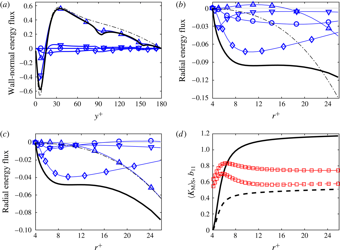
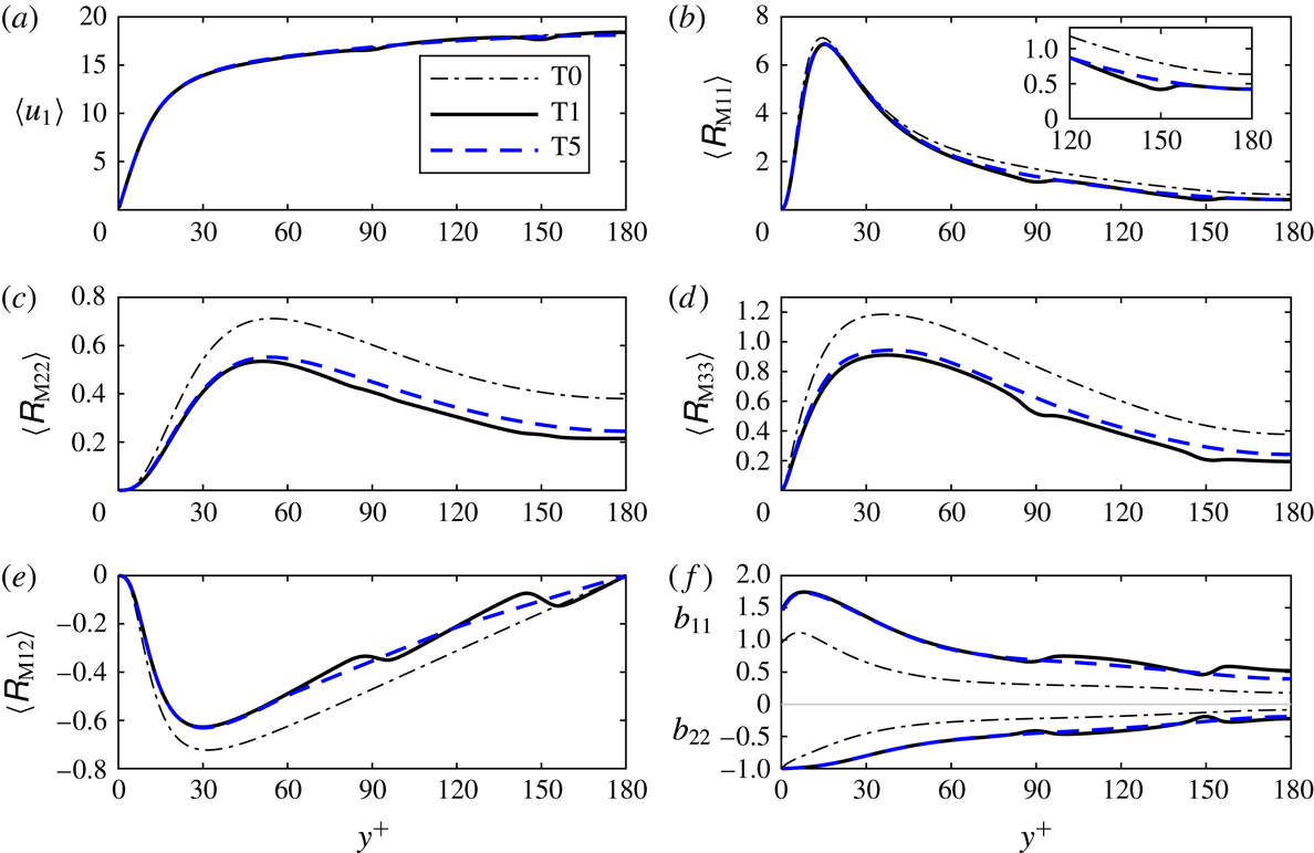
1 Introduction
The turbulence kinetic energy (TKE) of a turbulent air flow can be substantially reduced by a low volume fraction of small solid spherical particles. This phenomenon, also called turbulence attenuation, has been observed in many experiments of gas–solid turbulent flows, for example experiments of pipe flow (Tsuji, Morikawa & Shiomi Reference Tsuji, Morikawa and Shiomi1984), channel flow (Kulick, Fessler & Eaton Reference Kulick, Fessler and Eaton1994; Kussin & Sommerfeld Reference Kussin and Sommerfeld2002) and turbulence generated by woofers (Hwang & Eaton Reference Hwang and Eaton2006; Tanaka & Eaton Reference Tanaka and Eaton2010). In the latter work the local turbulence dissipation rate was directly measured and detected to be significantly enhanced near particles. Numerous point-particle simulations, simulations which do not resolve the boundary layers and wakes around the particles, confirmed the phenomenon of turbulence attenuation; see for example the simulations of isotropic turbulence by Squires & Eaton (Reference Squires and Eaton1990), Elghobashi & Truesdell (Reference Elghobashi and Truesdell1993) and Ferrante & Elghobashi (Reference Ferrante and Elghobashi2003), and the simulations of turbulent channel flow by Li et al. (Reference Li, McLaughlin, Kontomaris and Portela2001), Yamamoto et al. (Reference Yamamoto, Potthoff, Tanaka, Kajishima and Tsuji2001), Vreman (Reference Vreman2015) and Kuerten & Vreman (Reference Kuerten and Vreman2016). The last reference shows results for a dilute turbulent channel flow at friction Reynolds number 950 with 51 000 000 (colliding) particles. However, point-particle simulations seem to underpredict the amount of turbulence attenuation observed in experiments (Hwang & Eaton Reference Hwang and Eaton2006). This discrepancy has been attributed to oversimplicity of point-particle models (Burton & Eaton Reference Burton and Eaton2005; Hwang & Eaton Reference Hwang and Eaton2006), while part of the discrepancy for channel flows can be explained by wall roughness (Vreman Reference Vreman2015). The classical point-particle method was reviewed by Deen et al. (Reference Deen, van Sint Annaland, van der Hoef and Kuipers2007), Balachandar & Eaton (Reference Balachandar and Eaton2010) and Kuerten (Reference Kuerten2016), for example. An alternative method, the exact regularized point-particle method (Gualtieri et al. Reference Gualtieri, Picano, Sardina and Casciola2015), was employed by Gualtieri, Battista & Casciola (Reference Gualtieri, Battista and Casciola2017) and Battista et al. (Reference Battista, Gualtieri, Mollicone and Casciola2018) to simulate turbulence modulation in particle-laden homogeneous shear flow.
In contrast to point-particle simulations, particle-resolved direct numerical simulations (PR-DNS) do capture the boundary layers and wakes around the particles. In a PR-DNS no empirical correlation for the particle force is used, and the grid size near the particle is required to be much smaller than the particle diameter. PR-DNS is a very promising approach to investigating particle-laden turbulent flows in full detail, as reviewed by Tenneti & Subramaniam (Reference Tenneti and Subramaniam2014). Examples of flows for which PR-DNS has been used are one fixed particle in isotropic turbulence (Bagchi & Balachandar Reference Bagchi and Balachandar2003; Burton & Eaton Reference Burton and Eaton2005) or in channel flow (Zeng et al. Reference Zeng, Balachandar, Fischer and Najjar2008), multiple fixed particles in various turbulent flows (Botto & Prosperetti Reference Botto and Prosperetti2012; Vreman Reference Vreman2016) and freely moving particles or bubbles in decaying isotropic turbulence (ten Cate et al. Reference ten Cate, Derksen, Portela and van den Akker2004; Lucci, Ferrante & Elghobashi Reference Lucci, Ferrante and Elghobashi2010; Mehrabadi et al. Reference Mehrabadi, Tenneti, Garg and Subramaniam2015; Schneiders, Meinke & Schröder Reference Schneiders, Meinke and Schröder2017), in homogeneous turbulent shear flow (Tanaka Reference Tanaka2017), and in turbulent channel flow (Uhlmann Reference Uhlmann2008; García-Villalba, Kidanemariam & Uhlmann Reference García-Villalba, Kidanemariam and Uhlmann2012; Lu & Tryggvason Reference Lu and Tryggvason2013; Picano, Breugem & Brandt Reference Picano, Breugem and Brandt2015; Santarelli & Fröhlich Reference Santarelli and Fröhlich2015; Santarelli, Roussel & Fröhlich Reference Santarelli, Roussel and Fröhlich2016; Costa et al. Reference Costa, Picano, Brandt and Breugem2016). The last reference contains results of simulation of a dense turbulent channel flow with 640 000 neutrally buoyant particles.
The present work is in various respects a continuation of the work reported in Vreman (Reference Vreman2016), in which a body-fitted overset grid method was developed to perform the first PR-DNS of homogeneous isotropic turbulence globally attenuated by a low fraction of small particles. The particles were fixed, while the particle diameter
 $d_{p}$
was twice the Kolmogorov length scale
 $\unicode[STIX]{x1D702}$
, and the mean relative particle velocity (the mean velocity difference between particles and fluid) was zero. Analysis of the radial turbulence kinetic energy budget showed that on the particle surfaces, the turbulence dissipation rate was enhanced by a factor of 100. The turbulence kinetic energy was reduced in the entire flow, due to turbulent, pressure and viscous diffusion towards the particles. Surprisingly, point-particle simulations using the Schiller–Naumann drag law were shown to capture the turbulence attenuation found in the PR-DNS reasonably well, provided the fluid volume over which each particle force was distributed was sufficiently large.
In the present work, we use PR-DNS to investigate turbulence attenuation in turbulent channel flow modified by an array of reasonably small particles (
 $2\unicode[STIX]{x1D702}<d_{p}<3\unicode[STIX]{x1D702}$
), moving in the core region of the flow. Compared to the isotropic case, the analysis of the present case is substantially more complicated, because the turbulence is generated by mean shear and the mean relative particle velocity is non-zero. The streamwise velocity of the particle array is set to 90 % of the unladen bulk velocity, so that the particles move more slowly than the surrounding fluid. This particle velocity is an appropriate choice in the light of experiments of air turbulence in downward vertical gas–solid flow in which the particles also considerably lagged behind the fluid in the core region of the channel (Kulick et al.
Reference Kulick, Fessler and Eaton1994). In fact, the present system can be regarded as a simplification of a system in which small particles with a very large Stokes response time are regularly inserted into a vertical turbulent channel flow. The simplification is useful, because it allows particle–turbulence interaction to be studied without the complications caused by particle–particle and particle–wall collisions. Experiments of turbulent flow modified by a single fixed particle have been performed by Hoque et al. (Reference Hoque, Sathe, Joshi and Evans2016), while experiments of fluid flow through an array of fixed particles have been performed by Amoura et al. (Reference Amoura, Besnaci, Risso and Roig2017). In the latter case the turbulence was only generated by the (relatively large) particles, while following Risso et al. (Reference Risso, Roig, Amoura, Riboux and Billet2008), the velocity fluctuation was decomposed into a purely spatial and a temporal component, the spatial component accounting for the strong inhomogeneity of the flow around each sphere.
Before we further discuss the aim of the present study, we briefly review several other PR-DNS studies of spherical particles embedded in an otherwise standard turbulent channel flow. Zeng et al. (Reference Zeng, Balachandar, Fischer and Najjar2008) analysed the force on a single fixed particle at various distances from the wall for
 $d_{p}^{+}\geqslant 3.5$
and
 $Re_{\unicode[STIX]{x1D70F},0}=178$
, where
 $d_{p}^{+}$
is the particle diameter expressed in wall units of the unladen flow and
 $Re_{\unicode[STIX]{x1D70F},0}$
is the Reynolds number of the unladen flow, based on friction velocity and half the channel height. The grid size
 $h^{+}$
in the spectral element method was non-uniform and equal to 0.06 wall units at the particle surface. A vertical turbulent channel flow laden with a large number of free particles was simulated by Uhlmann (Reference Uhlmann2008). The turbulence intensity was strongly enhanced by the particles for
 $\unicode[STIX]{x1D6FC}_{p}=0.004$
,
 $d_{p}^{+}=8.5$
and
 $Re_{\unicode[STIX]{x1D70F}}=172$
, while the mean particle velocity was close to zero. An immersed boundary method was used with a uniform
 $h^{+}=d_{p}^{+}/13$
. For almost the same flow, particle acceleration statistics and the probability distribution of the hydrodynamic forces acting on the particles were computed by García-Villalba et al. (Reference García-Villalba, Kidanemariam and Uhlmann2012). The dynamics of nearly spherical bubbles in a turbulent channel flow was studied by Lu & Tryggvason (Reference Lu and Tryggvason2013), for
 $d_{p}^{+}=40$
,
 $\unicode[STIX]{x1D6FC}_{p}=0.03$
and
 $Re_{\unicode[STIX]{x1D70F},0}=250$
, using a front tracking method with uniform
 $h^{+}=d_{p}^{+}/26$
. For turbulent channel flow at
 $Re_{\unicode[STIX]{x1D70F},0}=180$
, laden with neutrally buoyant spheres, Picano et al. (Reference Picano, Breugem and Brandt2015) reported on the turbulence in the dense limit (
 $\unicode[STIX]{x1D6FC}_{p}=0.2$
and
 $d_{p}^{+}=20$
), while scaling laws for such suspensions were derived by Costa et al. (Reference Costa, Picano, Brandt and Breugem2016) for
 $d_{p}^{+}\geqslant 10$
,
 $\unicode[STIX]{x1D6FC}_{p}\geqslant 0.05$
, using an immersed boundary method with uniform
 $h^{+}=d_{p}^{+}/16$
. An enhancement of turbulence by spherical bubbles was reported by Santarelli & Fröhlich (Reference Santarelli and Fröhlich2015), who simulated a turbulent bubbly channel flow for
 $d_{p}^{+}=17$
,
 $\unicode[STIX]{x1D6FC}_{p}\geqslant 0.003$
and
 $Re_{\unicode[STIX]{x1D70F},0}=168$
, using an immersed boundary method with uniform
 $h^{+}=d_{p}^{+}/12$
. An analysis of the turbulence kinetic energy budget as a function of the distance to the wall revealed that the turbulence enhancement was generated by the so-called interfacial term (Santarelli et al.
Reference Santarelli, Roussel and Fröhlich2016).
As mentioned above, in the present paper PR-DNS of a turbulent channel flow modified by an array of spherical particles with a fixed streamwise velocity is considered. The particle diameter is set to
 $d_{p}^{+}=8$
, the overall particle volume fraction is
 $\unicode[STIX]{x1D6FC}_{p}=0.00075$
, and
 $Re_{\unicode[STIX]{x1D70F},0}=180$
. At the particle locations, the unladen Kolmogorov scale
 $\unicode[STIX]{x1D702}^{+}$
is approximately 3. This flow configuration lends itself to be simulated by the recently developed and well-validated overset grid method, applicable to cases with many (non-colliding) spherical particles (Vreman Reference Vreman2016, Reference Vreman2017). Due to radial stretching of the spherical body-fitted grid attached to each particle, the grid size at the particle surfaces is
 $d_{p}^{+}/31$
, which is sufficiently small to accurately capture the locally very high dissipation rate at the particle surfaces.
The aim of this study is to investigate the modification of the turbulence due to particles, in terms of quantities that are relevant for the production, transport and dissipation of turbulence. Another important topic, usage of the PR-DNS results to test and improve the point-particle simulation technique, will be presented in another paper. In the present paper, we will focus on TKE budgets: the standard (fixed-frame) TKE budget, which is a function of the wall distance only, and the budget in the frame of reference of the particles, which is called the moving-frame budget and is a function of the three spatial coordinates. The former is based on statistical averaging in the fixed frame, the channel frame of reference, and the latter on statistical averaging in the moving frame, the particle frame of reference. Statistics conditioned on the location in the particle frame of reference have been presented before: radial profiles of the turbulence dissipation at multiple sides of the particles in decaying isotropic turbulence (Lucci et al. Reference Lucci, Ferrante and Elghobashi2010), radial profiles of the TKE, its budget and all components of the velocity gradient around particles in forced isotropic turbulence (Vreman Reference Vreman2016) and three-dimensional (3-D) statistics of Reynolds stresses in particle-laden homogeneous turbulent shear flow (Tanaka Reference Tanaka2017).
We will use moving-frame averaging not only to obtain insight into the statistical structure of the turbulence around the particles, but also to distinguish between apparently laminar parts of the turbulence fluctuations near the particles and true turbulence. Each fixed-frame fluctuation can be decomposed into a moving-frame mean part, which is steady in the moving frame, and a moving-frame fluctuating part, which is unsteady in the moving frame. This implies a corresponding decomposition of the turbulence kinetic energy (Risso et al. Reference Risso, Roig, Amoura, Riboux and Billet2008; Amoura et al. Reference Amoura, Besnaci, Risso and Roig2017), and, as will be shown, also a corresponding decomposition of the turbulence dissipation rate and other terms in the TKE budget equation.
It is common in the literature to call the kinetic energy in the fixed-frame fluctuation turbulence kinetic energy, so we use this name too. However, we stress that only part of the fixed-frame TKE refers to ordinary turbulence energy, the energy in fluctuatuations resulting from complex instabilities in the fluid motion, in this case the energy in the moving-frame fluctuations. Another part of the fixed-frame TKE refers to the moving-frame mean part, which results from the displacement of fluid by the relative motion of the particles. One of the purposes of this paper is to show how the moving-frame mean part can affect the fixed-frame turbulence statistics. Although in this case the fluctuations that are steady and unsteady in the particle frame could be called pseudo-turbulence and true turbulence, respectively, pseudo-turbulence in general is a somewhat wider concept that could encompass fluctuations that are unsteady in the particle frame. Furthermore, pseudo-turbulence in the literature is usually quantified by the excess TKE of a bubbly flow over the TKE of the flow without the bubbles (Lance & Bataille Reference Lance and Bataille1991), but in our case the excess TKE of the flow with particles over the flow without particles turns out to be negative. For these reasons, we will avoid the term pseudo-turbulence in the rest of this paper.
The structure of this paper is as follows. The mathematical description and the validation of the PR-DNS are described in § 2. The 1-D fixed-frame Reynolds stresses and TKE budget are presented in § 3. The 3-D moving-frame Reynolds stresses and TKE budget are presented in § 4. In § 5, we apply the fixed-frame statistical averaging operator to the moving-frame budget, to condense the 3-D statistics to 1-D profiles that can be directly compared to the fixed-frame statistics from § 3. In § 6, we analyse the observed turbulence attenuation and the observed increase in anisotropy of the turbulence in further depth. We conclude the paper in § 7.
2 Mathematical description
In this section, we define the flow configuration, formulate the TKE equations in the fixed and moving frame, describe the numerical method, define simulation cases and show validation results.
New elements in this section and the related appendices are: (i) a derivation of the fluid-weighted TKE equation for general averaging operators, (ii) a derivation of the 3-D TKE equation in spherical coordinates and (iii) a body-fitted particle-resolved direct numerical simulation of a turbulent flow past more than 1000 particles.
2.1 Flow configurations
We consider an incompressible turbulent channel flow with bulk velocity
 $u_{b}$
and wall velocity zero, in which an array of
 $N_{par}$
solid non-rotating spherical particles is moving with a constant streamwise velocity,
 $0.9u_{b}$
. The dimensions of the channel,
 $u_{b}$
, and the viscosity
 $\unicode[STIX]{x1D708}$
are the same as in the reference flow without particles. The unladen reference simulation is case S2 from Vreman & Kuerten (Reference Vreman and Kuerten2014), a high-resolution long-time simulation of an incompressible turbulent channel flow in a standard domain and at standard Reynolds number. For explanatory reasons, we also consider a laminar channel flow, which has lower bulk velocity and is modified by an array of particles with velocity zero.
Streamwise, normal and spanwise directions are denoted by
 $x_{1}$
,
 $x_{2}$
and
 $x_{3}$
respectively, while time is denoted by
 $t$
. The channel half-width
 $H$
is equal to 1, the friction velocity of the unladen turbulent flow,
 $u_{\unicode[STIX]{x1D70F},0}$
, is equal to 1,
 $\unicode[STIX]{x1D708}=1/180$
, so that
 $Re_{\unicode[STIX]{x1D70F},0}=u_{\unicode[STIX]{x1D70F},0}H/\unicode[STIX]{x1D708}=180$
. All results in this paper are non-dimensionalized using
 $H$
and
 $u_{\unicode[STIX]{x1D70F},0}$
, which implies that
 $\unicode[STIX]{x1D708}=1/180$
in each case. The distance to the nearest wall is indicated by
 $y$
. The superscript
 $+$
applied to a length indicates a division by
 $1/180$
, the thickness of the viscous sublayer in the unladen flow. Thus
 $y^{+}=180(1-|x_{2}|)$
in each case. The spatial domain is given by
 $\unicode[STIX]{x1D6FA}_{0}=[0,L_{1}]\times [-1,1]\times [0,L_{3}]$
. The flow is periodic in the
 $x_{1}$
and
 $x_{3}$
directions. In the turbulent flow cases,
 $L_{1}=4\unicode[STIX]{x03C0}$
,
 $L_{3}=4\unicode[STIX]{x03C0}/3$
and
 $u_{b}=15.66$
, while in the laminar flow case
 $L_{1}=4\unicode[STIX]{x03C0}/18$
,
 $L_{3}=4\unicode[STIX]{x03C0}/36$
and
 $u_{b}=3$
. The translative velocity of the particles is indicated by
 $\boldsymbol{u}^{p}$
. In this paper, all particles have the same fixed
 $\boldsymbol{u}^{p}$
and zero angular velocity.
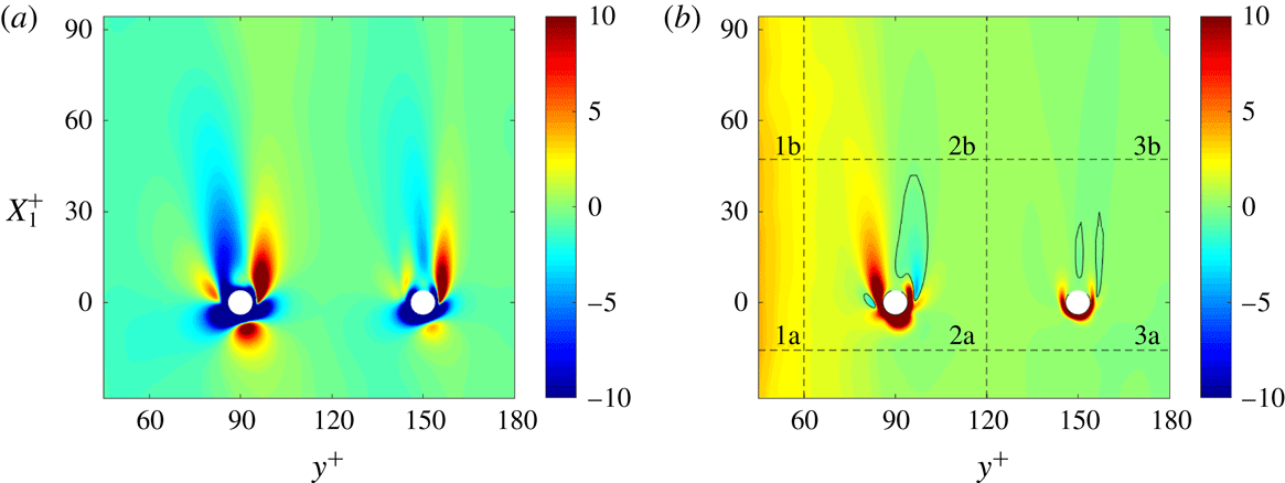
The structure of the particle array in three cross-sections of one-third of the flow domain in the streamwise direction (
 $0\leqslant x_{1}\leqslant L_{1}/3$
):
 $x_{3}=\unicode[STIX]{x03C0}/36\approx 0.087$
,
 $x_{3}=3\unicode[STIX]{x03C0}/36\approx 0.262$
and
 $x_{2}=-1/2$
. The demarcation lines indicate the much smaller flow domain of the laminar case.

The array in the turbulent flow contains 1728 spherical particles of diameter
 $d_{p}=2/45$
(
 $d_{p}^{+}=8$
) and is sketched in figure 1 (only the first two rows (8 particles) of this array are used in the laminar flow). The particle radius is denoted by
 $r_{0}=d_{p}/2$
, and the overall particle volume fraction is 0.00075. The particle configuration originates from a nearly cubical pattern of
 $36\times 4\times 12$
particles with pitch size
 $\unicode[STIX]{x03C0}/9$
in the streamwise and spanwise directions and pitch size
 $1/3$
in the normal direction. This nearly cubical pattern is modified by shifting the odd rows in the spanwise direction by
 $-\unicode[STIX]{x03C0}/36$
and the even rows by
 $\unicode[STIX]{x03C0}/36$
, in order to reduce the effect of neighbouring particles on the streamwise oriented wake behind each particle. The
 $x_{2}$
coordinates of the particles are
 $\pm 1/6$
and
 $\pm 1/2$
. From a statistical point of view there are only two types of particles: the particles at
 $y^{+}=90$
and those at
 $y^{+}=150$
, also indicated by
 $p=1$
and
 $p=2$
, respectively. Thus for each type there are many statistically equivalent particle positions (
 $1728/2$
), which is an advantage for the computation of accurate statistics in the particle frame of reference. More numerical and physical reasons for this specific configuration will be given in § 2.4.
A characterization of the unladen flow turbulence at the particle positions and a few particle Reynolds numbers based on unladen flow quantities.

Several unladen flow quantities and particle Reynolds numbers of the particles based on unladen flow velocities are specified in table 1 for the two distinct particle positions. The mean velocity, turbulence kinetic energy, turbulence dissipation rate and Kolmogorov length scale of the mean flow are denoted by
 $\overline{u}_{1,0}$
,
 $K_{0}$
,
 $\unicode[STIX]{x1D716}_{0}$
and
 $\unicode[STIX]{x1D702}_{0}$
, respectively. The particle Reynolds numbers due to the mean and fluctuating relative velocities are defined by
 $Re_{p,mean}=(\overline{u}_{1,0}-u_{1}^{p})d_{p}/\unicode[STIX]{x1D708}$
and
 $Re_{p,tur}=(2K_{0})^{1/2}d_{p}/\unicode[STIX]{x1D708}$
, respectively, where
 $\overline{u}_{1,0}$
and
 $K_{0}$
are the mean velocity and turbulence kinetic energy of the unladen flow. The total particle Reynolds number is defined by
 $R_{tot}=(Re_{p,mean}^{2}+Re_{p,tur}^{2})^{1/2}$
. For the laminar case, the (mean and total) particle Reynolds numbers are equal to 27 (
 $p=1$
) and 35 (
 $p=2$
). The corresponding relative velocities are obtained by dividing these Reynolds numbers by eight (
 $d_{p}/\unicode[STIX]{x1D708}=8/u_{\unicode[STIX]{x1D70F},0}$
).
2.2 Governing equations
The incompressible Navier–Stokes equations in Cartesian coordinates read
 $$\begin{eqnarray}\displaystyle & \displaystyle \unicode[STIX]{x2202}_{j}u_{j}=0, & \displaystyle\end{eqnarray}$$
 $$\begin{eqnarray}\displaystyle & \displaystyle \unicode[STIX]{x2202}_{t}u_{i}=-\unicode[STIX]{x2202}_{j}(u_{i}u_{j})-\unicode[STIX]{x2202}_{j}q+\unicode[STIX]{x1D708}\unicode[STIX]{x2202}_{j}^{2}u_{i}+a_{i}. & \displaystyle\end{eqnarray}$$
The symbols
 $\unicode[STIX]{x2202}_{t}$
and
 $\unicode[STIX]{x2202}_{j}$
denote
 $\unicode[STIX]{x2202}/\unicode[STIX]{x2202}t$
and
 $\unicode[STIX]{x2202}/\unicode[STIX]{x2202}x_{j}$
, respectively. Throughout the paper, the convention of summation over repeated indices in products is used, unless mentioned otherwise. The streamwise, wall-normal and spanwise Cartesian velocity components are denoted by
 $u_{1}$
,
 $u_{2}$
and
 $u_{3}$
, respectively. The symbol
 $q$
denotes the periodic part of the pressure divided by the fluid density. The streamwise component of the acceleration term
 $\boldsymbol{a}$
is equal to
 $(a_{1},0,0)$
, and
 $-a_{1}$
represents the non-periodic part of the streamwise component of the pressure gradient divided by the density. It only depends on time and is adjusted to maintain a constant
 $u_{b}$
, which is defined as the streamwise fluid velocity averaged over the fluid domain (
 $\unicode[STIX]{x1D6FA}_{0}$
minus the volumes occupied by the particles). The boundary conditions imposed on the fluid velocity at solid surfaces are
 $\boldsymbol{u}=0$
at the channel walls (
 $x_{2}=\pm 1$
) and
 $\boldsymbol{u}=\boldsymbol{u}^{p}$
at the surfaces of the particles.
For use in later sections, we define the fluid stress tensor
 $\unicode[STIX]{x1D748}$
and strain rate
 $\unicode[STIX]{x1D64E}$
:
 $$\begin{eqnarray}\displaystyle \unicode[STIX]{x1D70E}_{ij}=-q\unicode[STIX]{x1D6FF}_{ij}+2\unicode[STIX]{x1D708}\unicode[STIX]{x1D61A}_{ij},\quad \unicode[STIX]{x1D61A}_{ij}={\textstyle \frac{1}{2}}(\unicode[STIX]{x2202}_{j}u_{i}+\unicode[STIX]{x2202}_{i}u_{j}). & & \displaystyle\end{eqnarray}$$
The force exerted by the fluid stress
 $\unicode[STIX]{x1D70E}_{ij}$
on a particle is defined by
 $$\begin{eqnarray}\displaystyle F_{i}^{p}=\int _{S_{p}}\unicode[STIX]{x1D70E}_{ij}n_{j}\,\text{d}S, & & \displaystyle\end{eqnarray}$$
where
 $S_{p}$
is the surface of the particle, and
 $\boldsymbol{n}$
is the normal vector pointing into the fluid. Note that
 $F_{i}^{p}$
does not include the contribution of the non-periodic part of the streamwise pressure gradient. The actual force exerted by the fluid on the particle is equal to
 $\unicode[STIX]{x1D70C}F_{i}^{p}+\unicode[STIX]{x1D70C}a_{i}\unicode[STIX]{x03C0}d_{p}^{3}/6$
.
For each particle, a spherical coordinate system is attached to the particle centre (
 $\boldsymbol{x}^{p}$
) such that
 $$\begin{eqnarray}\displaystyle \boldsymbol{x}-\boldsymbol{x}^{p}=\left[\begin{array}{@{}l@{}}r\sin \unicode[STIX]{x1D703}\cos \unicode[STIX]{x1D719}\\ r\sin \unicode[STIX]{x1D703}\sin \unicode[STIX]{x1D719}\\ r\cos \unicode[STIX]{x1D703}\end{array}\right], & & \displaystyle\end{eqnarray}$$
where
 $r$
is the radial coordinate,
 $\unicode[STIX]{x1D703}$
the polar angle and
 $\unicode[STIX]{x1D719}$
the azimuthal angle. Thus the polar axis is aligned to the spanwise direction of the channel. The spherical velocity components in the frame of the reference moving with the particle are denoted by
 $u_{r}$
,
 $u_{\unicode[STIX]{x1D703}}$
and
 $u_{\unicode[STIX]{x1D719}}$
.
2.3 Numerical method
We employ the solver NSpheres (Vreman Reference Vreman2017), an MPI-parallel body-fitted incompressible Navier–Stokes solver for flows with multiple moving spheres. Around each spherical particle, the Navier–Stokes equations in spherical coordinates are solved on a staggered spherical grid attached to the particle. The spherical grids are overset on a staggered Cartesian grid. The Navier–Stokes equations are discretized using second-order accurate central differencing in space with third-order interpolations from Cartesian to spherical grids and vice versa. In principle, the interpolation data structure and interpolation coefficients are updated each time step. However, in the present case we avoid this by using a Cartesian grid that formally moves with the same constant velocity as the particle array. Thus we use the Galilean invariant property of the Navier–Stokes equations, and solve
 $u_{1}-u_{1}^{p}$
instead of
 $u_{1}$
, while we impose
 $u_{1}-u_{1}^{p}=-u_{1}^{p}$
at the channel walls. In the post-processing, we obtain
 $u_{1}$
by adding
 $u_{1}^{p}$
to the solution for
 $u_{1}-u_{1}^{p}$
. The temporal discretization is explicit, except for the
 $\unicode[STIX]{x1D719}$
direction on the spherical grids. Since, due to the viscous time step restriction, the time step is proportional to the square of the grid size, the formally first-order temporal discretization error reduces with the same rate as the spatial discretization error if the grid is refined. The pressure Poisson equation is iteratively solved using the BICGstab method (van der Vorst Reference van der Vorst1992) and a tolerance
 $10^{-5}$
for the maximum norm of the residual. The augmented matrix method (Henshaw Reference Henshaw1994; Vreman Reference Vreman2016) is used to overcome the singularity due to the formally unspecified absolute level of the pressure.
We call this numerical method, which is fully described in Vreman (Reference Vreman2017), numerical method A. For validation purposes, we additionally consider a slightly modified method, numerical method B, which differs in three aspects from method A. First, for the convective terms, the forward Euler temporal discretization is replaced by the second-order Adams–Bashforth method. The latter scheme was also used in Vreman (Reference Vreman2016), and its implementation is straightforward for cases in which the spherical grids do not move with respect to the Cartesian grid. Second, the tolerance for the maximum residual error in the Poisson equation is reduced to
 $10^{-6}$
. Third, another variant of the augmented matrix method is used, in which the augmented variable is added to the system before the matrix is normalized by dividing each row by its diagonal element. Thus in the system after normalization, the coefficient of the augmented variable in each row is no longer equal to 1, but equal to the reciprocal of the diagonal element before normalization. The coefficients of the augmented variable influence how (inevitable) errors in the velocity divergence are distributed in space. In method A, the velocity divergence error in the cells touching the poles does not converge formally to zero in the limit of zero grid size and zero tolerance, while it does in method B. However, in practice the divergence error at the poles occurring if method A is used can be so small that the maximum error of the divergence seems to converge to zero upon grid refinement: see Vreman (Reference Vreman2017). Furthermore, finite errors restricted to the poles are not expected to deteriorate the convergence of quantities integrated over a finite surface or a volume, since the surface or volume of the region where the divergence has a small finite value converges to zero upon grid refinement.
Overview of the particle-resolved simulations.

An overview of five particle-resolved simulations is shown in table 2. T stands for simulations of the turbulent flow and L for the simulation of the laminar flow. Case T1 is the main simulation, cases T2, T3 and T4 are introduced for validation purposes. The comparison in the next subsection will show that, for the present purposes, method A is sufficiently accurate (compared to method B), and that the discretization errors and statistical errors in the results of T1 are sufficiently small.
We proceed to specify the main simulation, T1, which was performed using numerical method A. The number of grid cells of the Cartesian grid is
 $1152\times 216\times 384$
. The uniform grid sizes in the streamwise and spanwise directions,
 $\unicode[STIX]{x0394}x_{1}^{+}$
and
 $\unicode[STIX]{x0394}x_{3}^{+}$
, are both equal to 1.96. The grid is stretched in the
 $x_{2}$
direction, such that
 $\unicode[STIX]{x0394}x_{2}^{+}$
linearly increases from approximately
 $0.5$
to
 $2$
for
 $0\leqslant y^{+}\leqslant 60$
over
 $48$
points and is equal to
 $2$
for
 $60\leqslant y^{+}\leqslant 180$
. Each spherical grid cell has
 $30\times 48\times 96$
cells and extends from
 $r_{0}^{+}=4$
to
 $r_{b}^{+}\approx 7r_{0}^{+}=28$
. The radius of the spherical holes in the Cartesian domain is set to
 $r_{a}=(r_{0}+r_{b})/2$
. The radial stretching function specified in Vreman (Reference Vreman2016) is used, such that the radial grid size
 $\unicode[STIX]{x0394}r^{+}$
is equal to
 $0.26$
at
 $r_{0}$
and
 $2$
at
 $r_{b}$
. The smallest radial grid size is called
 $h_{1}$
. The total number of grid cells (
 $N_{tot}$
) is approximately 343 million; 72 % of them belong to the spherical domains.
The total number of grid points in case T1 is not small, but if it had been simulated with one of the more common Cartesian methods for particle-resolved simulations, which typically use uniform cubical grids, 35 billion points would have been required to reach the same small mesh size near the particles. Thus, the overset grid method allows the number of grid points to be reduced by a factor of 100 for this volume fraction. However, the method needs an iterative method to solve the Poisson equation, and this consumes more than 90 % of the CPU time.
Simulation T1 was run on 432 processors. Each processor computed the flow on one block of the Cartesian grid and on the spherical grids of four particles. Thus the Cartesian domain was decomposed into 432 blocks, 36 blocks in the
 $x_{1}$
direction and 12 in the
 $x_{3}$
direction. The time step was equal to
 $3.5\times 10^{-5}$
, slightly lower than the viscous stability restriction. The velocity field was initialized using the parabolic profile and the perturbation specified in Vreman (Reference Vreman2014). This initial condition leads to a fast transition, such that the flow becomes turbulent well before
 $t=t_{1}=5$
. The end time of the simulation was
 $t=t_{2}=25$
. Complete spatial fields were stored each 0.07 time unit. The statistical averaging was performed by a post-processing program, which used all stored fields between
 $t=t_{1}$
and
 $t=t_{2}$
. The total simulation time of case T1 was approximately 0.7 million CPU hours, corresponding to approximately 10 weeks in wall clock time. In this case, the number of time steps was approximately 0.7 million, and on average the number of iterations of the Poisson solver was approximately 170 per time step.
The other cases do not require much additional explanation. All settings are the same as in case 1, except those mentioned in this paragraph. In case T2, each spherical and Cartesian grid is coarser by a factor of 2 in each direction, while the time step is four times larger. The end time could be taken larger in this case, because the simulation required much less CPU time than T1, due to the coarser grid and larger time step. Case T3 is based on the same run as case T1, but
 $t_{2}$
is smaller, such that the length of the time interval for statistical averaging (
 $t_{2}-t_{1}$
) is more than twice as small as in case 1. Case T4 is the same as case T3, except that method B has been used instead of method A. Furthermore, simulation T4 was started from the field at
 $t_{1}=5$
of case T3. Finally, L1 is the laminar case. The resolution and method in L1 are the same as in T1, but the initial condition of L1 is a parabolic profile without perturbations, and the domain is much smaller, such that precisely the first two rows (eight particles) of the particle array fit into the domain. The averaged quantities were computed from the last field. We verified that near the end of the simulation the solution was steady in the entire domain. Thus the last field of L1 does indeed correspond to a steady fully laminar flow.
2.4 Relevance of flow case
To limit the computing time without compromising on the near-wall resolution of the DNS, we did not place particles in the near-wall region, where the Cartesian grid is non-uniform. In the outer layer of the spherical grid around the particle
 $\unicode[STIX]{x0394}r^{+}\approx 2$
,
 $(r\unicode[STIX]{x0394}\unicode[STIX]{x1D703})^{+}\approx 2$
and the maximum
 $((r\sin \unicode[STIX]{x1D703})\unicode[STIX]{x0394}\unicode[STIX]{x1D719})^{+}\approx 2$
, thus if we placed a particle at for example
 $y^{+}=30$
there would be locations close to the wall where the wall-normal grid size would effectively be two wall units, while in the present case the wall-normal grid size at the wall is four times smaller (0.5 wall unit). Sufficient near-wall resolution would be obtained if the number of radial grid cells were increased by a factor of 4 in each direction or, alternatively, if the radial extent of the spherical grids were reduced in combination with a uniform Cartesian grid of grid size half a wall unit. The better option would probably be the latter one, but it would still imply a huge increase of the required CPU time (by approximately a factor of 15). Another option would be to use an immersed boundary method in combination with a fast Poisson solver on a uniform cubical grid of 5 billion cells (16 grid cells per particle diameter). However, this would probably reduce the accuracy of the numerical solution near the particles, for two reasons. First, the grid size near the particle surfaces would be twice as large as in the present T1. Second, for at least one common type of immersed boundary method, Stein, Guy & Thomases (Reference Stein, Guy and Thomases2017) have shown that the pressure and viscous stresses close to the surface of the particle do not converge pointwise to the correct values, although the particle force (which is not a pointwise quantity) does converge to the correct value.
Despite the restrictions imposed on location and velocity of the particles, the present flow case is interesting and new. The local 3-D inhomogeneity of the flow makes it a rich problem. It is a well-controlled configuration that facilitates an accurate computation of local statistics, even at locations very close to the particles. The particles are exposed to turbulence produced by real physical mechanisms in near-wall turbulence. As such this is a step forward compared with studies of particles in decaying isotropic turbulence (since the turbulence then depends on the initial condition) or forced isotropic turbulence (since the turbulence then depends on the forcing term). Our aim is to investigate how turbulent flow responds to particles, how energy exchange mechanisms are modified, in particular in the vicinity the particles. Even without particles in the near-wall region, the turbulence appears to be significantly modified in the entire flow (including the near-wall region). We wish to understand how a small volume fraction of particles can significantly influence the amount and character of the turbulence everywhere in the flow. We will find that the present PR-DNS confirms important findings and explanations hitherto only based on interpretations from experiments and point-particle simulations of vertical channel flows with freely moving particles (see §§ 3.1 and 6). Thus we expect that our conclusions regarding the 3-D statistical structure of the turbulence around the particles in the present configuration are somehow also valid for solid particles falling through turbulence, for example air turbulence generated by vertical channel walls (Kulick et al. Reference Kulick, Fessler and Eaton1994) or acoustic woofers at the edges of the set-up (Hwang & Eaton Reference Hwang and Eaton2006; Tanaka & Eaton Reference Tanaka and Eaton2010).
As mentioned in the Introduction, the present case of particles with a fixed velocity is a relevant limit for particles at high Stokes numbers caused by high inertia. In the copper particle experiments performed by Kulick et al. (Reference Kulick, Fessler and Eaton1994), the particle–fluid mass density ratio was approximately 7000, while the modified Stokes response time was roughly 8000 times larger than the wall unit time scale (
 $\unicode[STIX]{x1D6FF}_{\unicode[STIX]{x1D708}}/u_{\unicode[STIX]{x1D70F}}$
). We could have allowed free rotation of the particles in our case, but this would have been inconsistent with the previous argument that our case is relevant for cases with very high particle inertia. Furthermore, Zeng, Balachandar & Fischer (Reference Zeng, Balachandar and Fischer2005) found that the effect of sphere rotation on drag and lift forces is small, and it is the mean particle drag force that will be shown to cause most of the turbulence attenuation and anisotropy increase observed in the present case (§ 6).
For finite inertia and free motion of particles in the normal direction, the particles would be subjected to a larger range of the particle Reynolds number than in the present case. A larger range of the particle Reynolds number is interesting from a physical point of view, but higher particle Reynolds numbers lead to thinner no-slip particle boundary layers and the need for a smaller grid size near the particles. It is remarked that also in the present case the instantaneous particle Reynolds number is not constant. Based on the unladen flow velocity the (95 % probability) range of the instantaneous Reynolds number is from 0 to 50.
2.5 Definition of fixed-frame averaged quantities
The basic averaging operator in the fixed frame is denoted by an overbar and defined as the average over time and the two periodic directions (
 $x_{1}$
and
 $x_{3}$
). Thus the fixed-frame statistics are functions of the wall-normal direction only (
 $0\leqslant y^{+}\leqslant 180$
; for each
 $y^{+}$
, the statistics are based on the two planes
 $x_{2}=\pm (1-y^{+}/180)$
). The corresponding fluid phase-weighted averaging operator applied to an arbitrary function
 $f$
on
 $\unicode[STIX]{x1D6FA}_{0}$
is defined by
 $$\begin{eqnarray}\displaystyle \langle f\rangle _{}=\overline{\unicode[STIX]{x1D712}f}/\overline{\unicode[STIX]{x1D712}}, & & \displaystyle\end{eqnarray}$$
where
 $\unicode[STIX]{x1D712}$
is the commonly known indicator function of the fluid, equal to
 $1$
in the fluid and
 $0$
inside the solid phase. In addition, we define
 $\unicode[STIX]{x1D6FC}=\overline{\unicode[STIX]{x1D712}}$
, which is the volume fraction of the fluid after averaging, and we define the Reynolds stress tensor by
 $$\begin{eqnarray}\displaystyle \unicode[STIX]{x1D619}_{ij}=\langle u_{i}u_{j}\rangle _{}-\langle u_{i}\rangle _{}\langle u_{j}\rangle _{}. & & \displaystyle\end{eqnarray}$$
Often, the basic averaging operator is a Reynolds (or statistical) averaging operator, which can be the present overbar, averaging over time only (Ishii Reference Ishii1975) or averaging over an ensemble of realizations (Zhang & Prosperetti Reference Zhang and Prosperetti1997; Drew & Passman Reference Drew and Passman1999). These operators satisfy the Reynolds conditions, which are (i) linearity, (ii) invariance of constant fields, (iii) commutation with derivatives and (iv)
 $\overline{\overline{f_{1}}f_{2}}=\overline{f_{1}}\;\overline{f_{2}}$
for arbitrary functions
 $f_{1}$
and
 $f_{2}$
on
 $\unicode[STIX]{x1D6FA}_{0}$
. It is stressed that the fluid phase-weighted averaging operator does not inherit condition (iii), the commutation condition. Furthermore, if a local volume averaging operator is used, for example the operator defined by Anderson & Jackson (Reference Anderson and Jackson1967) and Jackson (Reference Jackson1997), an operator very similar to the Gaussian spatial convolution filter later used in large-eddy simulation, then the fourth Reynolds condition is not satisfied. However, for the fluid phase-weighted average, condition (iv) is satisfied, and this implies
 $\unicode[STIX]{x1D619}_{ij}=\langle u_{i}^{\prime }u_{j}^{\prime }\rangle _{}$
, where
 $u_{i}^{\prime }=u_{i}-\langle u_{i}\rangle$
is the velocity fluctuation.
The fixed-frame turbulence kinetic energy (TKE) is defined by
 $K_{}=(\unicode[STIX]{x1D619}_{ii})/2$
. For Reynolds averaging, the TKE equation for incompressible two-phase flow has been derived by Kataoka & Serizawa (Reference Kataoka and Serizawa1989). Using PR-DNS of turbulent bubbly channel flow, Santarelli et al. (Reference Santarelli, Roussel and Fröhlich2016) evaluated all the distinct terms in this equation, which are together called the TKE budget. In fact, the TKE equation can also be derived in an alternative way, without assuming incompressibility and Reynolds condition (iv); see appendix A. The resulting form is not only more general (also applicable in the context of local spatial averaging), but it also resembles how the actual evaluation of terms is performed in this paper, namely without explicit usage of any fluctuation field. We drop the phase subscript used in appendix A, and write the equations for the fluid phase in an incompressible particle-laden flow as
 $$\begin{eqnarray}\displaystyle 0=-\unicode[STIX]{x2202}_{j}(\unicode[STIX]{x1D6FC}\langle u_{j}\rangle _{}), & & \displaystyle\end{eqnarray}$$
 $$\begin{eqnarray}\displaystyle \unicode[STIX]{x2202}_{t}(\unicode[STIX]{x1D6FC}\langle u_{i}\rangle _{}) & = & \displaystyle -\unicode[STIX]{x2202}_{j}(\unicode[STIX]{x1D6FC}\langle u_{i}\rangle _{}\langle u_{j}\rangle _{})-\unicode[STIX]{x2202}_{j}(\unicode[STIX]{x1D6FC}\unicode[STIX]{x1D619}_{ij})\nonumber\\ \displaystyle & & \displaystyle -\,\unicode[STIX]{x2202}_{i}(\unicode[STIX]{x1D6FC}\langle q\rangle _{})+\unicode[STIX]{x2202}_{j}(2\unicode[STIX]{x1D6FC}\unicode[STIX]{x1D708}\langle \unicode[STIX]{x1D61A}_{ij}\rangle _{})-\overline{\unicode[STIX]{x1D70E}_{ij}\unicode[STIX]{x2202}_{j}\unicode[STIX]{x1D712}}+\unicode[STIX]{x1D6FC}\langle a_{i}\rangle _{},\end{eqnarray}$$
 $$\begin{eqnarray}\displaystyle \unicode[STIX]{x2202}_{t}K_{}=C_{}+P_{}+T_{}+\unicode[STIX]{x1D6F1}_{}+D_{}-\unicode[STIX]{x1D716}_{}+I+B_{}. & & \displaystyle\end{eqnarray}$$
The last equation is the TKE equation, in which
 $C_{}$
is convective transport,
 $P_{}$
turbulence production,
 $T_{}$
turbulent transport,
 $\unicode[STIX]{x1D6F1}_{}$
pressure diffusion,
 $D_{}$
viscous diffusion,
 $\unicode[STIX]{x1D716}_{}$
turbulence dissipation,
 $I=I_{1}+I_{2}$
the interfacial term and
 $B_{}$
body-force production:
 $$\begin{eqnarray}\displaystyle & \displaystyle C_{}=-\frac{1}{\unicode[STIX]{x1D6FC}}\unicode[STIX]{x2202}_{j}(\unicode[STIX]{x1D6FC}\langle u_{j}\rangle K), & \displaystyle\end{eqnarray}$$
 $$\begin{eqnarray}\displaystyle & \displaystyle P_{}=-\unicode[STIX]{x1D619}_{ij}\unicode[STIX]{x2202}_{j}\langle u_{i}\rangle _{}, & \displaystyle\end{eqnarray}$$
 $$\begin{eqnarray}\displaystyle & \displaystyle T_{}=-\frac{1}{\unicode[STIX]{x1D6FC}}\unicode[STIX]{x2202}_{j}\left(\frac{1}{2}\unicode[STIX]{x1D6FC}\langle u_{i}u_{i}u_{j}\rangle _{}-\frac{1}{2}\unicode[STIX]{x1D6FC}\langle u_{i}\rangle \langle u_{i}\rangle \langle u_{j}\rangle -\unicode[STIX]{x1D6FC}\langle u_{i}\rangle _{}\unicode[STIX]{x1D619}_{ij}-\unicode[STIX]{x1D6FC}\langle u_{j}\rangle _{}K_{}\right), & \displaystyle\end{eqnarray}$$
 $$\begin{eqnarray}\displaystyle & \displaystyle \unicode[STIX]{x1D6F1}_{}=-\frac{1}{\unicode[STIX]{x1D6FC}}\unicode[STIX]{x2202}_{j}(\unicode[STIX]{x1D6FC}\langle qu_{j}\rangle _{}-\unicode[STIX]{x1D6FC}\langle q\rangle _{}\langle u_{j}\rangle _{}), & \displaystyle\end{eqnarray}$$
 $$\begin{eqnarray}\displaystyle & \displaystyle D_{}=\frac{2\unicode[STIX]{x1D708}}{\unicode[STIX]{x1D6FC}}\unicode[STIX]{x2202}_{j}(\unicode[STIX]{x1D6FC}\langle u_{i}\unicode[STIX]{x1D61A}_{ij}\rangle _{}-\unicode[STIX]{x1D6FC}\langle u_{i}\rangle _{}\langle \unicode[STIX]{x1D61A}_{ij}\rangle _{}), & \displaystyle\end{eqnarray}$$
 $$\begin{eqnarray}\displaystyle & \displaystyle \unicode[STIX]{x1D716}_{}=2\unicode[STIX]{x1D708}(\langle \unicode[STIX]{x1D61A}_{ij}\unicode[STIX]{x1D61A}_{ij}\rangle _{}-\langle \unicode[STIX]{x1D61A}_{ij}\rangle _{}\langle \unicode[STIX]{x1D61A}_{ij}\rangle _{}), & \displaystyle\end{eqnarray}$$
 $$\begin{eqnarray}\displaystyle & \displaystyle I_{1}=\frac{1}{\unicode[STIX]{x1D6FC}}(\langle u_{i}\rangle _{}\overline{\unicode[STIX]{x1D70E}_{ij}\unicode[STIX]{x2202}_{j}\unicode[STIX]{x1D712}}-\overline{u_{i}\unicode[STIX]{x1D70E}_{ij}\unicode[STIX]{x2202}_{j}\unicode[STIX]{x1D712}}), & \displaystyle\end{eqnarray}$$
 $$\begin{eqnarray}\displaystyle & \displaystyle I_{2}=-\langle \unicode[STIX]{x1D70E}_{ij}\rangle _{}(\langle \unicode[STIX]{x2202}_{j}u_{i}\rangle _{}-\unicode[STIX]{x2202}_{j}\langle u_{i}\rangle _{}), & \displaystyle\end{eqnarray}$$
 $$\begin{eqnarray}\displaystyle & \displaystyle B_{}=\langle u_{i}a_{i}\rangle _{}-\langle u_{i}\rangle _{}\langle a_{i}\rangle _{}. & \displaystyle\end{eqnarray}$$
This form is the basis for the numerical implementation of the fixed-frame TKE equation in the present paper. The gradient of the indicator function is a generalized function (Drew & Passman Reference Drew and Passman1999),
 $$\begin{eqnarray}\displaystyle \unicode[STIX]{x2202}_{j}\unicode[STIX]{x1D712}=n_{j}\unicode[STIX]{x1D6FF}_{fs}, & & \displaystyle\end{eqnarray}$$
where
 $\boldsymbol{n}$
is the normal vector perpendicular to the interface, pointing from the solid to the fluid region, and
 $\unicode[STIX]{x1D6FF}_{fs}$
a delta function on
 $\unicode[STIX]{x1D6FA}_{0}$
, infinitely large on the fluid–solid interface and zero otherwise. The non-commutation term
 $I_{2}$
can be rewritten as
 $$\begin{eqnarray}\displaystyle I_{2}=-\frac{1}{\unicode[STIX]{x1D6FC}}\langle \unicode[STIX]{x1D70E}_{ij}\rangle _{}(\langle u_{i}\rangle _{}\unicode[STIX]{x2202}_{j}\unicode[STIX]{x1D6FC}-\overline{u_{i}\unicode[STIX]{x2202}_{j}\unicode[STIX]{x1D712}}). & & \displaystyle\end{eqnarray}$$
Further discussion of the formulation of the fixed-frame TKE equation and the description of its numerical implementation can be found in appendix B.
2.6 Definition of moving-frame averaged quantities
An analysis based on averaging in the (non-rotating) frame of reference of the particle (the moving frame) provides useful insight into the mechanisms of a turbulent particle-laden flow. If the particles do not move relative to each other, the averaging operator required for such an analysis is relatively simple. Thus in the frame of reference moving with
 $u_{i}^{p}$
, we define
 $\langle \cdot \rangle _{\text{M}}$
as the operator that averages over time and over all particle frames that are statistically equivalent. In the present configuration, there are only two statistically different particle frames (
 $p=1$
and
 $p=2$
). The statistical quantities due to this averaging are 3-D functions, constant in time, but dependent on all three spatial coordinates. For any fluid variable
 $f$
, the fluctuation
 $f^{\prime \prime }$
is defined by
 $f^{\prime \prime }=f-\langle f\rangle _{\text{M}}$
. The fluid velocity in the frame of reference of the particle is denoted by
 $w_{i}=u_{i}-u_{i}^{p}$
.
The averaged equations for the fluid phase in the translative frame of reference of particle
 $p$
are given by
 $$\begin{eqnarray}\displaystyle \unicode[STIX]{x2202}_{j}\langle w_{j}\rangle _{\text{M}}=0, & & \displaystyle\end{eqnarray}$$
 $$\begin{eqnarray}\displaystyle \unicode[STIX]{x2202}_{t}\langle w_{i}\rangle _{\text{M}} & = & \displaystyle -\unicode[STIX]{x2202}_{j}(\langle w_{i}\rangle _{\text{M}}\langle w_{j}\rangle _{\text{M}})-\unicode[STIX]{x2202}_{j}\unicode[STIX]{x1D619}_{\text{M}ij}\nonumber\\ \displaystyle & & \displaystyle -\,\unicode[STIX]{x2202}_{i}\langle q\rangle _{\text{M}}+2\unicode[STIX]{x1D708}\unicode[STIX]{x2202}_{j}\langle \unicode[STIX]{x1D61A}_{ij}\rangle _{\text{M}}+\langle a_{i}\rangle _{\text{M}}+\unicode[STIX]{x2202}_{t}\langle u_{i}^{p}\rangle _{\text{M}},\end{eqnarray}$$
 $$\begin{eqnarray}\displaystyle \unicode[STIX]{x2202}_{t}K_{\text{M}}=C_{\text{M}}+P_{\text{M}}+T_{\text{M}}+\unicode[STIX]{x1D6F1}_{\text{M}}+D_{\text{M}}-\unicode[STIX]{x1D716}_{\text{M}}+J_{\text{M}}+B_{\text{M}}. & & \displaystyle\end{eqnarray}$$
In these equations,
 $$\begin{eqnarray}\displaystyle \unicode[STIX]{x1D619}_{\text{M}ij}=\langle w_{i}w_{j}\rangle _{\text{M}}-\langle w_{i}\rangle _{\text{M}}\langle w_{j}\rangle _{\text{M}}=\langle w_{i}^{\prime \prime }w_{j}^{\prime \prime }\rangle _{\text{M}}, & & \displaystyle\end{eqnarray}$$
while the turbulence kinetic energy
 $K_{\text{M}}$
is
 $\unicode[STIX]{x1D619}_{\text{M}ii}/2$
, and the terms in the TKE equation (2.24) are defined by
 $$\begin{eqnarray}\displaystyle & \displaystyle C_{\text{M}}=-\unicode[STIX]{x2202}_{j}(\langle w_{j}\rangle _{\text{M}}K_{\text{M}}), & \displaystyle\end{eqnarray}$$
 $$\begin{eqnarray}\displaystyle & \displaystyle P_{\text{M}}=-\unicode[STIX]{x1D619}_{\text{M}ij}\unicode[STIX]{x2202}_{j}\langle w_{i}\rangle _{\text{M}}, & \displaystyle\end{eqnarray}$$
 $$\begin{eqnarray}\displaystyle T_{\text{M}} & = & \displaystyle -\unicode[STIX]{x2202}_{j} (\!{\textstyle \frac{1}{2}}\langle w_{i}w_{i}w_{j}\rangle _{\text{M}}-{\textstyle \frac{1}{2}}\langle w_{i}\rangle _{\text{M}}\langle w_{i}\rangle _{\text{M}}\langle w_{j}\rangle _{\text{M}}\nonumber\\ \displaystyle & & \displaystyle -\,\langle w_{i}\rangle _{\text{M}}\unicode[STIX]{x1D619}_{\text{M}ij}-\langle w_{j}\rangle _{\text{M}}K_{\text{M}}\!)=-{\textstyle \frac{1}{2}}\unicode[STIX]{x2202}_{j}\langle w_{i}^{\prime \prime }w_{i}^{\prime \prime }w_{j}^{\prime \prime }\rangle _{\text{M}},\end{eqnarray}$$
 $$\begin{eqnarray}\displaystyle \unicode[STIX]{x1D6F1}_{\text{M}}=-\unicode[STIX]{x2202}_{j}(\langle qw_{j}\rangle _{\text{M}}-\langle q\rangle _{\text{M}}\langle w_{j}\rangle _{\text{M}})=-\unicode[STIX]{x2202}_{j}\langle q^{\prime \prime }w_{j}^{\prime \prime }\rangle _{\text{M}}, & & \displaystyle\end{eqnarray}$$
 $$\begin{eqnarray}\displaystyle D_{\text{M}} & = & \displaystyle \unicode[STIX]{x1D708}\unicode[STIX]{x2202}_{j}^{2}K_{\text{M}}-\unicode[STIX]{x1D708}(\langle (\unicode[STIX]{x2202}_{i}w_{j})(\unicode[STIX]{x2202}_{j}w_{i})\rangle _{\text{M}}-\langle \unicode[STIX]{x2202}_{i}w_{j}\rangle _{\text{M}}\langle \unicode[STIX]{x2202}_{j}w_{i}\rangle _{\text{M}})\nonumber\\ \displaystyle & = & \displaystyle 2\unicode[STIX]{x1D708}\unicode[STIX]{x2202}_{j}(\langle w_{i}\unicode[STIX]{x1D61A}_{ij}\rangle _{\text{M}}-\langle w_{i}\rangle _{\text{M}}\langle \unicode[STIX]{x1D61A}_{ij}\rangle _{\text{M}})=2\unicode[STIX]{x1D708}\unicode[STIX]{x2202}_{j}\langle w_{i}^{\prime \prime }\unicode[STIX]{x1D61A}_{ij}^{\prime \prime }\rangle _{\text{M}},\end{eqnarray}$$
 $$\begin{eqnarray}\displaystyle & \displaystyle \unicode[STIX]{x1D716}_{\text{M}}=2\unicode[STIX]{x1D708}(\langle \unicode[STIX]{x1D61A}_{ij}\unicode[STIX]{x1D61A}_{ij}\rangle _{\text{M}}-\langle \unicode[STIX]{x1D61A}_{ij}\rangle _{\text{M}}\langle \unicode[STIX]{x1D61A}_{ij}\rangle _{\text{M}})=2\unicode[STIX]{x1D708}\langle \unicode[STIX]{x1D61A}_{ij}^{\prime \prime }\unicode[STIX]{x1D61A}_{ij}^{\prime \prime }\rangle _{\text{M}}, & \displaystyle\end{eqnarray}$$
 $$\begin{eqnarray}\displaystyle & \displaystyle J_{\text{M}}=-\langle w_{i}\unicode[STIX]{x2202}_{t}u_{i}^{p}\rangle _{\text{M}}+\langle w_{i}\rangle _{\text{M}}\langle \unicode[STIX]{x2202}_{t}u_{i}^{p}\rangle _{\text{M}}=-\langle w_{i}^{\prime \prime }\unicode[STIX]{x2202}_{t}{u_{i}^{p}}^{\prime \prime }\rangle _{\text{M}}, & \displaystyle\end{eqnarray}$$
 $$\begin{eqnarray}\displaystyle & \displaystyle B_{\text{M}}=\langle w_{i}a_{i}\rangle _{\text{M}}-\langle w_{i}\rangle _{\text{M}}\langle a_{i}\rangle _{\text{M}}=\langle w_{i}^{\prime \prime }a_{i}^{\prime \prime }\rangle _{\text{M}}. & \displaystyle\end{eqnarray}$$
In each of the equations (2.25) and (2.28)–(2.33), the form in which the terms are numerically evaluated is given first, followed by an expression in terms of fluctuations. The former expressions would also provide a valid TKE equation if
 $\langle \cdot \rangle _{\text{M}}$
did not satisfy the fourth Reynolds condition. The term
 $C_{\text{M}}$
is the convection term, and
 $P_{\text{M}}$
is turbulence production,
 $T_{\text{M}}$
turbulent transport,
 $\unicode[STIX]{x1D6F1}_{\text{M}}$
pressure diffusion,
 $D_{\text{M}}$
viscous diffusion,
 $\unicode[STIX]{x1D716}_{\text{M}}$
turbulence dissipation,
 $J_{\text{M}}$
a term due to particle acceleration and
 $B_{\text{M}}$
body-force production. In the present case, the left-hand sides of (2.23)–(2.24) are zero, and
 $\unicode[STIX]{x2202}_{t}u_{i}^{p}=0$
so that
 $J_{\text{M}}=0$
. Apart from the occurrence of
 $J_{\text{M}}$
, this TKE equation has the same form as the single-phase TKE equation for cases with a 3-D mean flow.
Since there are only two statistically different types of particles, the 3-D domain can be decomposed in 1728/2 statistically equivalent rectangular blocks. The size of each block is
 $L_{1}/18\times H\times L_{3}/24$
. The output of the post-processing program is a series of statistical quantities defined on a 3-D domain of the size of one block, which we call the reference block. Each moving-frame statistical quantity is determined at the cell centres of the active Cartesian cells and at the cell centres of the spherical cells. In addition to the evaluations of each term at the cell centres, the terms
 $D_{\text{M}}$
and
 $\unicode[STIX]{x1D716}_{\text{M}}$
are also explicitly computed at the centres of the cell faces on the particle surfaces. The numerical implementation of the moving-frame TKE equation is further described in appendix C. The numerical implementation employs the TKE equation in spherical coordinates, which is also derived in this appendix since we could not find that form in the literature.
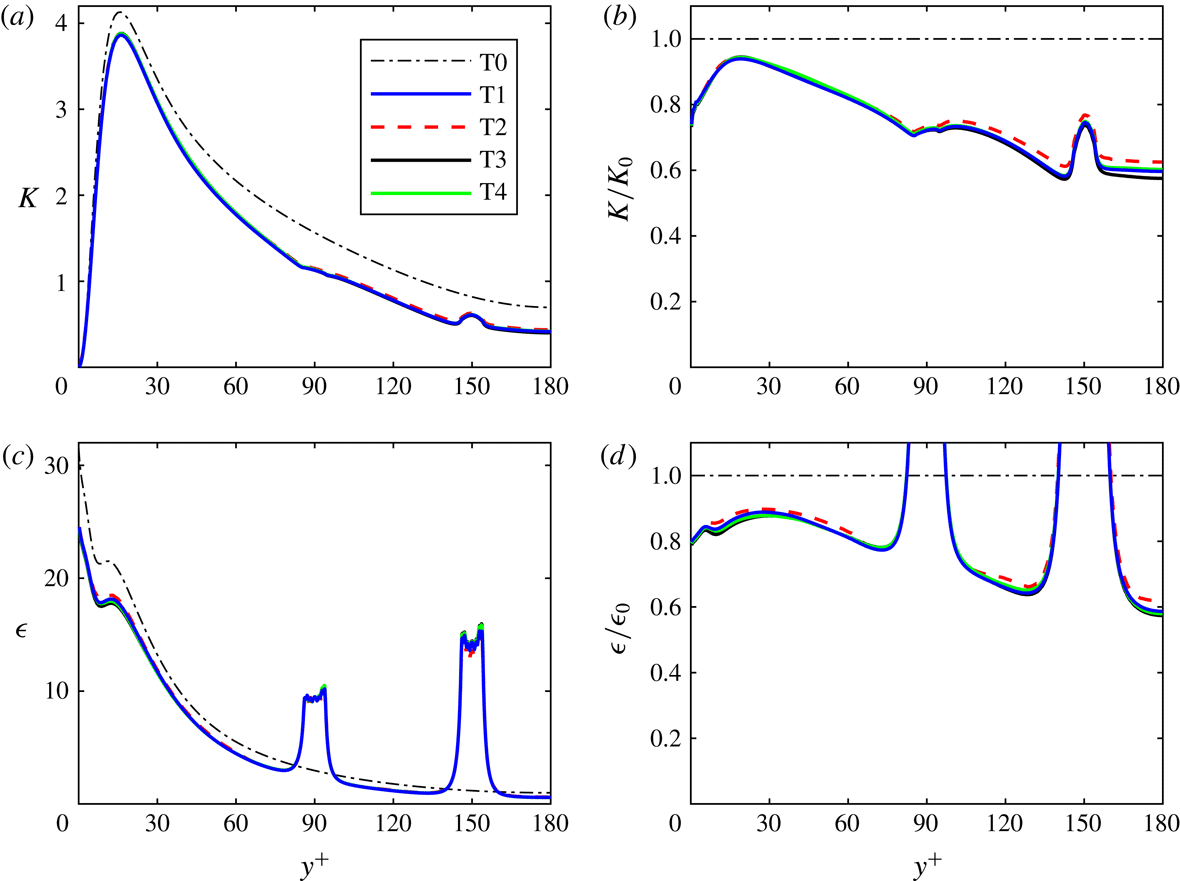
Fixed-frame statistics from cases T1 (blue solid), T2 (red dashed), T3 (black solid), T4 (green solid) and the unladen case T0 (thin black dash-dotted). (a,b) Turbulence kinetic energy
 $K$
before (a) and after (b) normalization with its unladen counterpart (
 $K_{0}$
). (c,d) Turbulence dissipation rate before (c) and after (d) normalization with its unladen counterpart (
 $\unicode[STIX]{x1D716}_{0}$
).

2.7 Validation
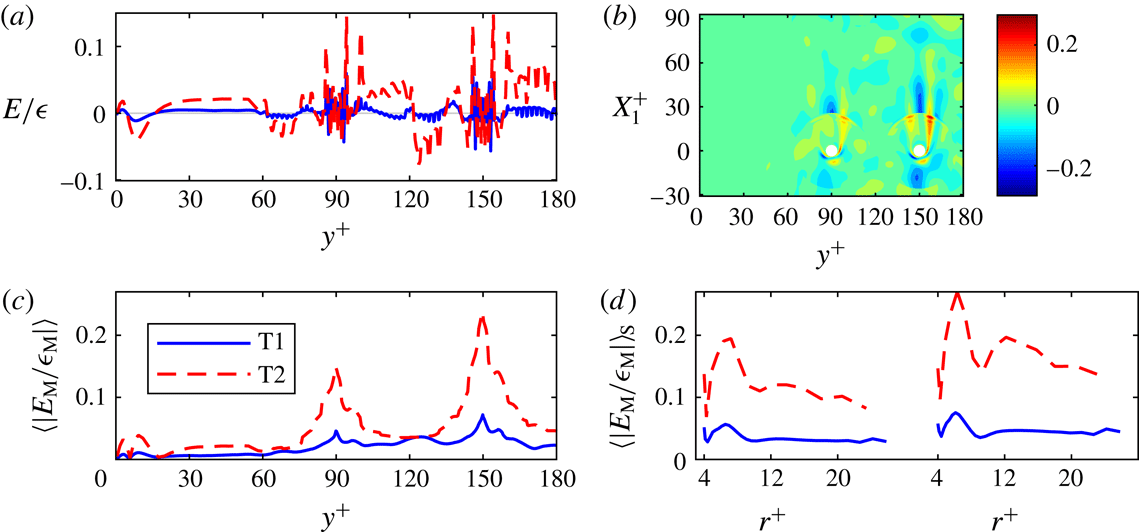
Representative results of simulations T1, T2, T3 and T4 of the turbulent case are shown in figures 2 and 3 and table 3. Case T0 denotes the unladen turbulent channel flow, while
 $E$
and
 $E_{\text{M}}$
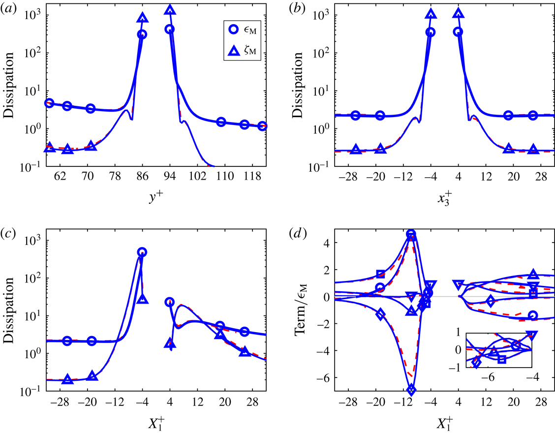
denote the fixed-frame and moving-frame budget errors, the sums of all terms on the right-hand sides of the discretized forms of (2.10) and (2.24), respectively. The reasonably small discrepancies between fine-grid simulation T1 and coarse-grid simulation T2 are primarily caused by discretization errors in T2 and to a lesser extent caused by statistical errors in T1. Furthermore, profiles shown in the next sections will confirm that also for the individual Reynolds stresses and the individual budget terms the differences between T1 and T2 are quite small for the fixed-frame terms (figures 5 and 6) and reasonably small for the moving-frame terms (figures 13 and 14). It is concluded that the simulation on the finest grid, T1, is sufficiently accurate for our purposes. A more extensive discussion of the validation results can be found in appendix D.
Statistics of the forces on the particles. The numbers for cases T1 and L1 have been multiplied by 100. For T2, T3 and T4, the relative differences with respect to T1 are shown. Root-mean-square denoted by r.m.s.

(a) Relative fixed-frame budget error
 $E/\unicode[STIX]{x1D716}$
. (b) Relative moving-frame budget error
 $E_{\text{M}}/\unicode[STIX]{x1D716}_{\text{M}}$
in a symmetry plane cutting through the particles for case T1. (c) Planar average of
 $|E_{\text{M}}/\unicode[STIX]{x1D716}_{\text{M}}|$
. (d) Spherical surface average of
 $|E_{\text{M}}/\unicode[STIX]{x1D716}_{\text{M}}|$
as a function of the radius, which is the distance to the particle centre, for particles at
 $y^{+}=90$
(left subplot) and for particles at
 $y^{+}=150$
(right subplot). (a,c,d) Fine-grid case T1 (blue solid) and coarse-grid case T2 (red dashed).

3 Fixed-frame TKE budget and related statistics
All results in this section are based on fixed-frame averaging, more precisely fluid-weighted averaging in the channel frame of reference, as defined in § 2.5. This is the standard way of defining continuous-phase statistics in the multiphase literature. The kinetic energy in the fluctuations resulting from this type of averaging is the TKE (
 $K$
). In multiphase literature,
 $K$
is conventionally called the turbulence kinetic energy (of the phase under consideration). It is therefore logical that the first of our results sections is devoted to the fixed-frame TKE budget. However, we stress that, despite its name,
 $K$
does not correspond to ordinary turbulence (chaotic motion caused by complex flow instabilities) only. This is confirmed by § 3.2, in which we show that a laminar flow can have a non-zero
 $K$
. How large the apparently non-turbulent parts in quantities commonly regarded and used as turbulence statistics in dispersed multiphase flows are, will be clarified in § 5. Although we are aware that in the present section the label turbulence in the names of quantities may be a bit misleading, we think that, after the explanation above and in the Introduction, we can stick to the conventional terminology.
The new findings in this section are: (i) the observation of significant attenuation of the TKE in a particle-resolved DNS of a particle-laden channel flow at small particle volume fraction, (ii) visual grid independence of each individual term of the full fixed-frame TKE budget in an inhomogeneous turbulent flow past particles and (iii) the observation that conventional fluid-weighted averaging can lead to a large interfacial budget term and a large turbulence dissipation rate in both turbulent and laminar flow.
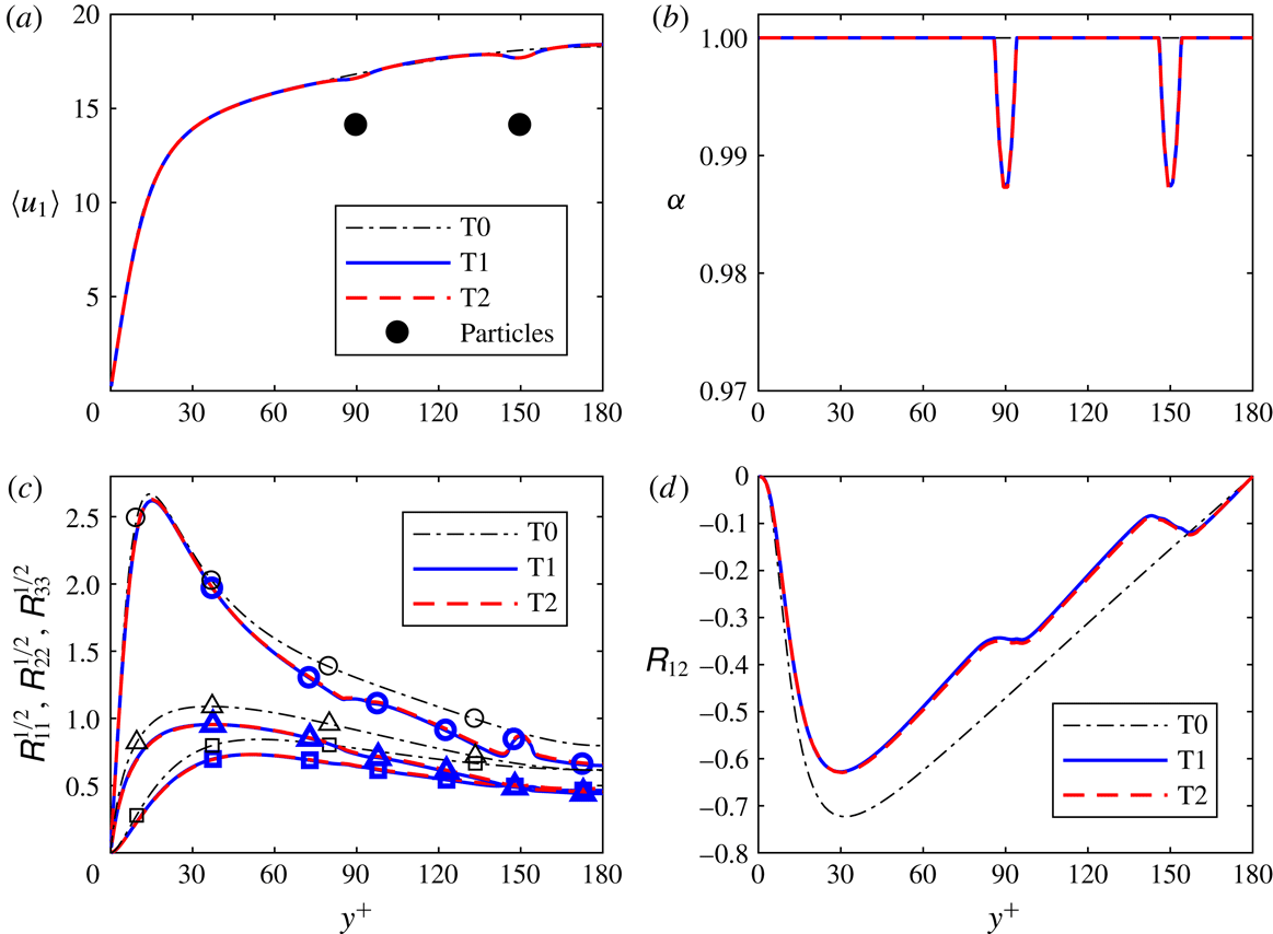
Fixed-frame statistics. Mean fluid velocity and particle velocity (a), mean particle volume fraction (b), streamwise (circles), wall-normal (squares) and spanwise (triangles) turbulence intensities (c) and Reynolds shear stress (d). Fine-grid case T1 (blue solid), coarse-grid case T2 (red dashed) and unladen case T0 (thin black dash-dotted). The velocity and positions of the particles are indicated by two black circles of diameter
 $d_{p}^{+}$
.

3.1 Fixed-frame results of the turbulent case
Before we show the results for the TKE budget of the turbulent case, we show and discuss the results of a number of basic statistical quantities. The mean velocity and fluid volume fraction profiles are shown in figure 4. The mean velocity seems to be largely unaffected by the particles, a finding that is consistent with experimental results (Kulick et al.
Reference Kulick, Fessler and Eaton1994). The wall-friction velocity
 $u_{\unicode[STIX]{x1D70F}}$
, derived from the mean velocity profile, and the corresponding
 $Re_{\unicode[STIX]{x1D70F}}$
are
 $0.979$
and 176, respectively (for both T1 and T2), 2 % smaller than the unladen values,
 $u_{\unicode[STIX]{x1D70F},0}$
and
 $Re_{\unicode[STIX]{x1D70F},0}$
. Since in this case the particles are concentrated at two
 $y^{+}$
locations, we do see a somewhat lower mean fluid velocity around these particle locations. The overall particle volume fraction is 0.00075, but due to the structure of the array, the mean particle volume fraction, which is a function of
 $y^{+}$
, peaks at 0.0128 (at
 $y^{+}=90$
and
 $y^{+}=150$
). According to figure 4(c), all three turbulence intensities are attenuated, while the wall-normal and spanwise intensities decrease relatively more than the streamwise one. These observations are also consistent with experimental findings (Kulick et al.
Reference Kulick, Fessler and Eaton1994; Kussin & Sommerfeld Reference Kussin and Sommerfeld2002). Furthermore, the Reynolds shear stress is weakened by the particles (figure 4
d).
Despite the small changes in the mean velocity profile, the turbulence kinetic energy
 $K$
is significantly attenuated for all
 $y^{+}$
; see figure 2 in the previous section. The strongest attenuation is observed at the centre line, where
 $K$
has reduced to approximately 60 % of its unladen value. Surprisingly, a clear local maximum of
 $K$
is observed at
 $y^{+}=150$
, while a bump in the profile is observed
 $y^{+}=90$
. Figure 4(c) reveals that the local maximum in
 $K$
at the second particle location is mainly caused by
 $\unicode[STIX]{x1D619}_{11}$
, the streamwise component of the Reynolds stress. Later on in this paper, we will explain the local maxima of
 $K$
and
 $\unicode[STIX]{x1D619}_{11}$
at
 $y^{+}=150$
(§§ 3.2 and 5). Figure 2 also shows a decrease of the turbulence dissipation rate
 $\unicode[STIX]{x1D716}$
, but not at all locations; around the
 $y^{+}$
locations of the particles,
 $\unicode[STIX]{x1D716}$
is strongly enhanced.
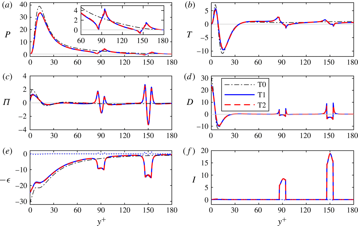
Fixed-frame turbulence kinetic energy budget: (a) standard production (the inset zooms in on the channel core), (b) turbulent transport, (c) pressure diffusion, (d) viscous diffusion, (e) turbulence dissipation and (f) interface term
 $I$
. Fine-grid case T1 (blue solid), coarse-grid case T2 (red dashed) and unladen case T0 (thin black dash-dotted). The blue dotted lines in (e,f) represent the small cross-term contribution to the turbulence dissipation rate (
 $\unicode[STIX]{x1D708}\langle (\unicode[STIX]{x2202}_{i}u_{j})^{\prime }(\unicode[STIX]{x2202}_{j}u_{i})^{\prime }\rangle$
) and the small commutator contribution to the interfacial term (
 $I_{2}$
), respectively.

The profiles of all terms in the fixed-frame TKE budget are shown in figure 5. Compared to the unladen flow, all terms are reduced in the near-wall region, except the interfacial term
 $I$
of course, which is zero in the unladen flow and in the near-wall region of the particle-laden flow. The term
 $B$
, which is negligible (
 ${<}0.002$
), and the convection term
 $C$
, which is zero because (2.8) implies
 $\langle u_{2}\rangle _{}=0$
, are not shown. Furthermore, we observe that a large part of the strongly enhanced turbulence dissipation rate near the particles is compensated by the large and positive
 $I$
, which apparently represents production of turbulence kinetic energy by the presence of particles. This is consistent with the findings of Santarelli et al. (Reference Santarelli, Roussel and Fröhlich2016), who found
 $I\approx \unicode[STIX]{x1D716}$
in the core of the channel, for turbulent channel flow with (freely moving) bubbles at larger particle volume fraction (
 ${\geqslant}0.003$
) and at much larger particle Reynolds number. A positive
 $I$
means that the particles produce turbulence kinetic energy. One could imagine that fluctuating bubbles inject energy into the TKE equation. However, in the present case the particle velocity fluctuation is zero. Thus the large interfacial term must have another cause in this case.
At this point, it is useful to consider the composition of the interfacial term in more detail. On particle surfaces, the instantaneous velocity
 $\boldsymbol{u}$
is equal to the velocity of the particles
 $u_{i}^{p}$
. Since the latter is constant and the same for all particles, the two contributions to the interfacial term,
 $I_{1}$
and
 $I_{2}$
(2.17)–(2.18), can be simplified to
 $$\begin{eqnarray}\displaystyle & \displaystyle I_{1}=\frac{1}{\unicode[STIX]{x1D6FC}}(\langle u_{i}\rangle _{}-u_{i}^{p})\overline{\unicode[STIX]{x1D70E}_{ij}\unicode[STIX]{x2202}_{j}\unicode[STIX]{x1D712}}, & \displaystyle\end{eqnarray}$$
 $$\begin{eqnarray}\displaystyle & \displaystyle I_{2}=-\frac{1}{\unicode[STIX]{x1D6FC}}(\langle u_{i}\rangle _{}-u_{i}^{p})\langle \unicode[STIX]{x1D70E}_{ij}\rangle _{}\unicode[STIX]{x2202}_{j}\unicode[STIX]{x1D6FC}. & \displaystyle\end{eqnarray}$$
Apparently,
 $I_{1}$
and
 $I_{2}$
are inner products of vectors with
 $\langle \boldsymbol{u}\rangle _{}-\boldsymbol{u}^{p}$
, the mean relative velocity between the phases, so that they both vanish if the mean relative velocity is zero. Thus, for particles with constant velocity, the turbulence kinetic energy produced by the interfacial term is a direct consequence of a non-zero mean relative velocity. According to equation (B 5) in appendix B,
 $I_{1}$
and
 $I_{2}$
are both zero if
 $\unicode[STIX]{x2202}_{j}\unicode[STIX]{x1D712}=0$
, i.e. for all
 $y^{+}$
for which the plane parallel to the wall is not intersected by an interfacial surface. Thus, in this case,
 $I$
is precisely non-zero in the two intervals with width
 $d_{p}$
centred around the two particle locations. The form of (3.2) suggests that
 $I_{2}$
is small if the variation of
 $\unicode[STIX]{x1D6FC}$
is small. Indeed, figure 5(f) shows that
 $I_{2}$
is negligible compared to
 $I$
.
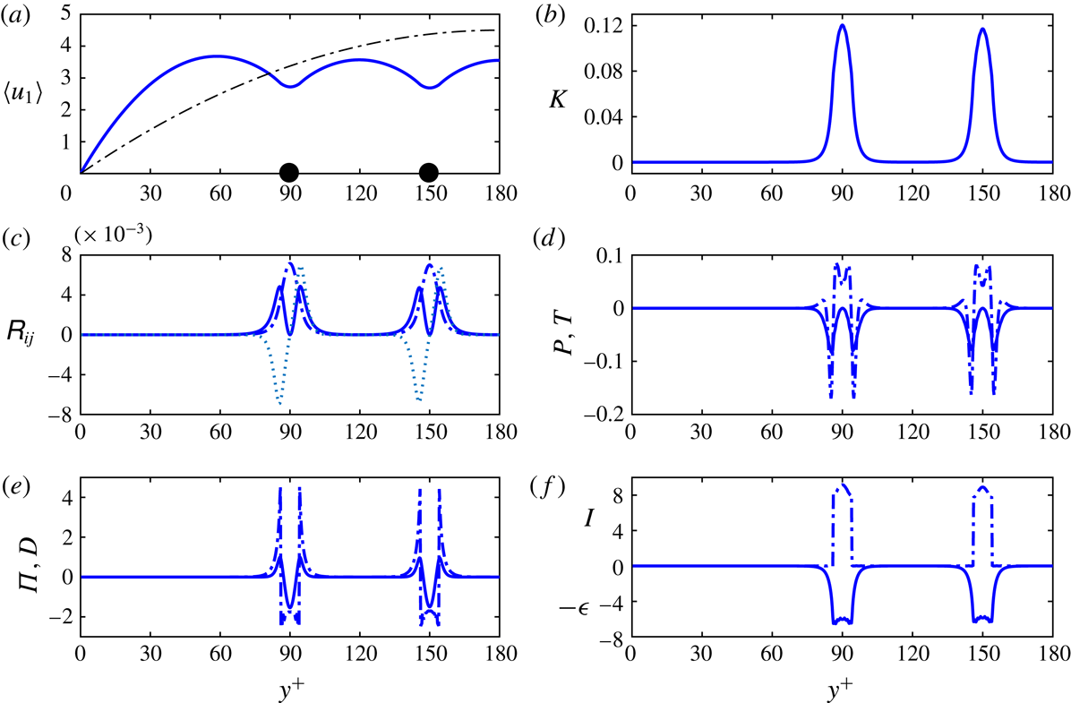
Fixed-frame statistics for the laminar case L1: (a) mean streamwise velocity (blue solid), (b) turbulence kinetic energy, (c) Reynolds stresses
 $\unicode[STIX]{x1D619}_{22}$
(solid),
 $\unicode[STIX]{x1D619}_{33}$
(dash-dotted) and
 $\unicode[STIX]{x1D619}_{12}$
(dotted), (d) standard production (solid) and turbulent transport (dash-dotted), (e) pressure diffusion (solid) and viscous diffusion (dash-dotted) and (f) turbulence dissipation (solid) and interfacial term (dash-dotted). Panel (a) also includes the unladen laminar velocity profile (thin dash-dotted) and the particle velocity (black circles).

The placement of all particles at two specific
 $x_{2}$
positions leads to sudden changes in the different particle terms. The particle volume fraction
 $1-\unicode[STIX]{x1D6FC}$
is not continuously differentiable at the edges of the particles (the particle locations plus or minus
 $d_{p}/2$
). This gives rise to strong discontinuities in
 $I$
at these locations, discontinuities which are balanced by the discontinuities in the viscous diffusion term
 $D$
. Another effect is that the non-zero transport terms,
 $T$
,
 $\unicode[STIX]{x1D6F1}$
and
 $D$
, change sign around the particles, and that even the production changes sign, at least near
 $y^{+}=150$
(see inset of figure 5
a). Thus the particles have a strong locally disturbing effect on all conventional terms in the turbulence kinetic energy equation. We will discuss the local effects of particles on the surrounding turbulence in more detail in §§ 4 and 6.
The quantity
 $\overline{\unicode[STIX]{x1D70E}_{ij}\unicode[STIX]{x2202}_{j}\unicode[STIX]{x1D712}}$
, which appears in (3.1) and (2.17), is proportional to the force exerted by the fluid on the particles as a function of
 $x_{2}$
. In fact
 $-\overline{\unicode[STIX]{x1D70E}_{ij}\unicode[STIX]{x2202}_{j}\unicode[STIX]{x1D712}}$
is the interfacial term in the mean momentum (2.9), and therefore we call this term the mean drag loading (the mean density of the drag force exerted by the particles on the fluid). We derive an estimate for the level of
 $\overline{\unicode[STIX]{x1D70E}_{ij}\unicode[STIX]{x2202}_{j}\unicode[STIX]{x1D712}}$
around
 $x_{2}^{p}$
. For this purpose, we define a thin volumetric slice
 $V_{s}=[0,L_{1}]\times [-x_{2}^{p}-r_{0},x_{2}^{p}+r_{0}]\times [0,L_{3}]$
around
 $x_{2}^{p}$
. The particle volume fraction in this slice is denoted by
 $\unicode[STIX]{x1D6FC}_{s}$
and is equal to
 $432V_{p}/(d_{p}L_{1}L_{3})$
, where
 $V_{p}=\unicode[STIX]{x03C0}d_{p}^{3}/6$
. For
 $x_{2}\approx x_{2}^{p}$
,
 $$\begin{eqnarray}\displaystyle \overline{\unicode[STIX]{x1D70E}_{ij}\unicode[STIX]{x2202}_{j}\unicode[STIX]{x1D712}} & {\approx} & \displaystyle \frac{1}{d_{p}}\int _{x_{2}^{p}-r_{0}}^{x_{2}^{p}+r_{0}}\overline{\unicode[STIX]{x1D70E}_{ij}\unicode[STIX]{x2202}_{j}\unicode[STIX]{x1D712}}\,\text{d}x_{2}\nonumber\\ \displaystyle & = & \displaystyle \frac{1}{d_{p}L_{1}L_{3}(t_{2}-t_{1})}\int _{t_{1}}^{t_{2}}\int _{0}^{L_{1}}\int _{x_{2}^{p}-r_{0}}^{x_{2}^{p}+r_{0}}\int _{0}^{L_{3}}(\unicode[STIX]{x1D70E}_{ij}\unicode[STIX]{x2202}_{j}\unicode[STIX]{x1D712})\,\text{d}x_{3}\,\text{d}x_{2}\,\text{d}x_{1}\,\text{d}t\nonumber\\ \displaystyle & = & \displaystyle \frac{432}{d_{p}L_{1}L_{3}}\text{mean}(F_{i}^{p})=\frac{\unicode[STIX]{x1D6FC}_{s}}{V_{p}}\text{mean}(F_{i}^{p}).\end{eqnarray}$$
Since the mean of
 $F_{1}^{p}$
is expected to have the same sign as
 $\langle u_{1}\rangle -u_{1}^{p}$
, and the wall-normal and spanwise components of the mean relative velocity are zero, the interfacial term
 $I\approx I_{1}$
in the budget is expected to be positive. In particular, equation (3.1) is approximated by
 $$\begin{eqnarray}\displaystyle I_{1}\approx \frac{\unicode[STIX]{x1D6FC}_{s}}{V_{p}}(\langle u_{1}\rangle -u_{1}^{p})\;\text{mean}(F_{1}^{p})\approx 185(\langle u_{1}\rangle -u_{1}^{p})\;\text{mean}(F_{1}^{p}), & & \displaystyle\end{eqnarray}$$
for
 $x_{2}\approx x_{2}^{p}$
. This equation would in fact reduce to the model for the interfacial term in bubbly flows proposed by Throsko & Hassan (Reference Throsko and Hassan2001) and tested by Santarelli et al. (Reference Santarelli, Roussel and Fröhlich2016) if we replaced
 $F_{1}^{p}$
by the standard model expression for the particle drag force. To evaluate this approximation for
 $I_{1}$
, we use the PR-DNS values for
 $F_{1}^{p}$
listed in table 3. Furthermore, we use the PR-DNS values for
 $\langle u_{1}\rangle -u_{1}^{p}$
at
 $y^{+}=90$
and
 $y^{+}=150$
, which are 2.53 and 3.60 respectively. Thus we obtain
 $I\approx I_{1}\approx 7.6$
and
 $I\approx 16.8$
, and the comparison with figure 5(f) shows that these are indeed good approximations of the average heights of the two peaks in the interfacial term.
3.2 Fixed-frame results of the laminar case
In the previous section, we observed a surprising peak in
 $K$
around
 $y^{+}=150$
, a very strong enhancement of
 $\unicode[STIX]{x1D716}$
around
 $y^{+}=90$
and
 $y^{+}=150$
, and in the same regions a large production of turbulence kinetic energy by the interfacial term even though the particle velocity fluctuation is zero. Are these remarkable observations caused by true turbulence or do laminar effects play a role? How much of
 $K$
and
 $\unicode[STIX]{x1D716}$
is truly turbulent? While definitive answers to these questions will be given in § 5, we address a related question in this subsection, namely whether the remarkable features also persist in a laminar channel flow past a particle array. We therefore consider the results of case L1, in which, in order to keep the flow laminar and the relative particle velocity roughly the same, the fluid bulk velocity was reduced to 3, and the velocity of the particle array was set to 0. The fluid-weighted averaging operator
 $\langle \cdot \rangle$
was applied to the steady state reached by this flow.
The results of simulation L1 are shown in figure 6. It appears that the turbulence kinetic energy is non-zero around the particles, although the flow is laminar and steady. This is in line with the work of Mehrabadi et al. (Reference Mehrabadi, Tenneti, Garg and Subramaniam2015), who observed a non-zero TKE in PR-DNS of laminar flow past an array of fixed particles. Due to the laminar flow disturbance around the particle, each velocity component is subject to spatial variation in planes parallel to the wall, which implies a non-zero spatial fluctuation with respect to the planar average. According to figure 6(b,c),
 $K$
is much larger than
 $\unicode[STIX]{x1D619}_{22}$
and
 $\unicode[STIX]{x1D619}_{33}$
, which implies
 $\unicode[STIX]{x1D619}_{11}\approx 2K$
. This very strong anisotropy must be due to the wakes behind the particles, which reduce the streamwise velocity considerably below
 $\langle u_{1}\rangle$
in a rather large region. Because
 $\unicode[STIX]{x1D619}_{22}$
is very small, the Reynolds shear stress
 $\unicode[STIX]{x1D619}_{12}$
is also small (although it is non-zero: see figure 6
c). This also explains the peak near the second particle position and the bump around the first particle position in figure 2(a). The latter is a bump because the level of the increase in
 $K$
due to laminar effects is rather small compared to the background turbulence at the first particle position.
It appears that the interfacial term and the turbulence dissipation rate are larger than
 $\unicode[STIX]{x1D6F1}$
and
 $D$
and much larger than
 $P$
and
 $T$
. Thus in this case we have
 $I\approx \unicode[STIX]{x1D716}$
(the interfacial production of
 $K$
is balanced by the dissipation of
 $K$
), although the profile of
 $I$
is thinner and has a slightly larger peak than that of
 $\unicode[STIX]{x1D716}$
. In view of the modest value of
 $K$
(only 0.12), it is surprising how large
 $I$
and
 $\unicode[STIX]{x1D716}$
are near the particle locations, of the same order as in the turbulent flow around
 $y^{+}=90$
(figure 5
e,f).
With respect to the local distortions by the particles, there is a strong similarity between cases L1 and T1, not only for
 $I$
and
 $\unicode[STIX]{x1D716}$
, but also for the shape distortions of
 $P$
and the transport terms around the particle positions. Thus laminar effects can significantly contribute to
 $K$
and
 $\unicode[STIX]{x1D716}$
, and several similarities between L1 and T1 suggest that laminar effects have an important effect on turbulence statistics in the turbulent case too.
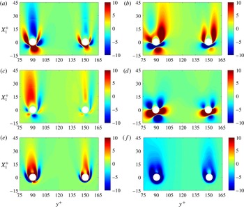
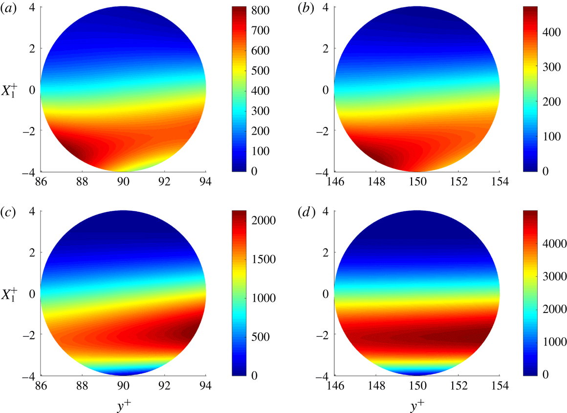
4 Moving-frame TKE budget and related statistics
In this section we characterize the 3-D structure of the moving-frame TKE budget and related statistics. We recall that the moving-frame statistics are based on averaging over time and statistically equivalent blocks so that we only have to consider the reference 3-D block defined in § 2.6. Moreover, we only look at the turbulent case since in the laminar case the moving-frame TKE is zero everywhere (this was verified).
The new elements in this section are: (i) a detailed picture of all terms in the moving-frame TKE budget, taking the full 3-D inhomogeneity of the turbulence in the particle frame of reference into account, (ii) the finding that the production term is strongly negative in a region in front of the particle and a corresponding physical explanation in terms of the local turbulence anisotropy, (iii) the observation that despite the overall attenuation of the turbulence there are regions near the particles where turbulence production is significantly enhanced, (iv) a comparison between the turbulence and mean dissipation rates near the particles (both are increased by orders of magnitude on the particle surfaces) and (v) the definition and computation of a particle surface viscous length scale (by analogy to the channel wall viscous length scale).
4.1 Mean flow and Reynolds stresses
Figure 7 shows the contours of the streamwise and wall-normal mean velocity components and the turbulence kinetic energy
 $K_{M}$
on the symmetry plane
 $X_{3}=0$
of the reference 3-D block (
 $X_{i}=x_{i}-x_{i}^{p}$
). This symmetry plane includes the centres of the two statistically different particles. In this plane,
 $\langle u_{3}\rangle _{\text{M}}=0$
, and
 $\unicode[STIX]{x2202}_{3}\langle u_{1}\rangle _{\text{M}}=0$
. In the planes
 $X_{2}=0$
through the particles, the structure of
 $\langle u_{3}\rangle _{\text{M}}$
is similar to the structure of
 $\langle u_{2}\rangle _{\text{M}}$
in figure 7(b). In figure 7(c), we observe a region of relatively low turbulence kinetic energy around each particle. These regions are elongated in the streamwise direction and include the rather long wakes behind the particles. The Reynolds shear stress
 $\unicode[STIX]{x1D619}_{\text{M}12}$
in this plane (figure 7
d) has, on top of the negative background Reynolds shear stress, a quadrant type of structure around each particle: negative near the left front and right rear and positive near the right front and left rear. The structures at the rear occur in the free shear layers at both sides of the wake behind each particle and their sign tends to be opposite to the sign of the local shear component
 $\langle \unicode[STIX]{x1D61A}_{12}\rangle _{\text{M}}$
.
Contours of moving-frame statistics in the plane
 $X_{3}=0$
(case T1). (a) Mean streamwise velocity
 $\langle u_{1}\rangle _{\text{M}}-u_{1}^{p}$
. (b) Mean wall-normal velocity
 $\langle u_{2}\rangle _{\text{M}}$
. (c) Turbulence kinetic energy
 $K_{\text{M}}$
. (d) Reynolds shear stress
 $\unicode[STIX]{x1D619}_{\text{M}12}$
.

Contours of moving-frame Reynolds stresses in the plane
 $X_{3}=0$
(case T1). (a)
 $\unicode[STIX]{x1D619}_{\text{M}11}$
. (b)
 $\unicode[STIX]{x1D619}_{\text{M}22}$
. (c)
 $\unicode[STIX]{x1D619}_{\text{M}33}$
. (d) Anisotropy coefficient
 $b_{\text{M}11}$
.

The four non-zero components of the Cartesian Reynolds stress tensor in the plane
 $X_{3}=0$
are shown in figure 8. The distortion of the turbulence by the particles is clearly not entirely symmetric about the
 $y^{+}=90$
and
 $y^{+}=150$
axes through the particles. All three diagonal components are substantially suppressed around the particles, while the wake structures created by the particles persist further downstream for
 $\unicode[STIX]{x1D619}_{\text{M}11}$
than for
 $\unicode[STIX]{x1D619}_{\text{M}22}$
and
 $\unicode[STIX]{x1D619}_{\text{M}33}$
(the latter two quantities recover more quickly than
 $\unicode[STIX]{x1D619}_{\text{M}11}$
and the mean streamwise velocity). However, somewhat downstream of the particles (around
 $X_{1}^{+}\approx 10$
) and on the right side (
 $y^{+}\approx 100$
for
 $p=1$
and
 $y^{+}\approx 160$
for
 $p=2$
) we observe local maxima of
 $\unicode[STIX]{x1D619}_{\text{M}11}$
(see figure 8
a, less easy to discern for
 $p=2$
than for
 $p=1$
). These local maxima appear inside a region of enhanced anisotropy of the turbulence (see figure 8
d), where the streamwise component of the anisotropy tensor,
 $b_{\text{M}11}=-1+3\unicode[STIX]{x1D619}_{\text{M}11}/(\unicode[STIX]{x1D619}_{\text{M}11}+\unicode[STIX]{x1D619}_{\text{M}22}+\unicode[STIX]{x1D619}_{\text{M}33})$
, is shown. We observe that the anisotropy is strongly modified near the particles, but while
 $b_{\text{M}11}$
is increased in some regions, it is reduced in other regions. Near the fronts and the rears of the particles,
 $b_{\text{M}11}$
approaches
 $-1$
since there
 $u_{1}^{\prime \prime }$
is the particle wall-normal component and therefore vanishes faster than
 $u_{2}^{\prime \prime }$
and
 $u_{3}^{\prime \prime }$
if the particle surface is approached. At the sides of the particle in this plane,
 $u_{2}^{\prime \prime }$
is the particle wall-normal component. Thus at those locations values of
 $b_{\text{M}22}$
approach
 $-1$
and, as a consequence,
 $b_{\text{M}11}$
(and
 $b_{\text{M}33}$
) increase. We observe that the low
 $b_{\text{M}11}$
at the rears and the high
 $b_{\text{M}11}$
at the sides are transported downstream. Thus the wake has a long core of relatively low
 $b_{\text{M}11}$
, embraced by a hull of relatively high
 $b_{\text{M}11}$
.
Moving-frame TKE budget in the plane
 $X_{3}=0$
(case T1). Positive values of production
 $P_{\text{M}}$
(red dash-dotted, contour levels 2, 5, 20 and 100). Negative production
 $P_{\text{M}}$
(blue dashed) and minus the dissipation rate
 $-\unicode[STIX]{x1D716}_{\text{M}}$
(blue solid), both for contour levels
 $-$
2,
 $-$
5,
 $-$
20 and
 $-$
100. The arrows represent the total transport flux vector (for each coordinate direction, the odd numbered points are skipped).

4.2 TKE budget
An overview of the moving-frame TKE budget in the same plane is shown in figure 9. The dissipation is enhanced around the particles, but the production is too, while negative production occurs as well. Arrows are used to visualize the total transport flux vector, the vector inside the divergence in
 $C_{\text{M}}+T_{\text{M}}+\unicode[STIX]{x1D6F1}_{\text{M}}+D_{\text{M}}$
(
 $C_{\text{M}}$
is also a transport term, because it can be written in divergence form). We observe a background flow of turbulence kinetic energy in the positive
 $x_{1}$
and positive
 $x_{2}$
directions. This background flow is dominated by
 $\langle w_{1}\rangle K_{\text{M}}$
in the
 $x_{1}$
direction and by
 $\langle u_{i}^{\prime \prime }u_{i}^{\prime \prime }u_{2}^{\prime \prime }\rangle _{\text{M}}/2$
in the
 $x_{2}$
direction.
Contours of moving-frame TKE budget in the plane
 $X_{3}=0$
(case T1), all clipped to the range
 $[-10,10]$
; most dark red (dark blue) regions contain peaks much higher than 10 (much lower than
 $-$
10). (a) Convection term
 $C_{\text{M}}$
. (b) Production term
 $P_{\text{M}}$
. (c) Turbulent transport term
 $T_{\text{M}}$
. (d) Pressure diffusion term
 $\unicode[STIX]{x1D6F1}_{\text{M}}$
. (e) Viscous diffusion term
 $D_{\text{M}}$
. (f) Minus turbulence dissipation rate
 $-\unicode[STIX]{x1D716}_{\text{M}}$
.

Extrema of the terms in the moving average budget and
 $\unicode[STIX]{x1D701}_{\text{M}}=2\unicode[STIX]{x1D708}\langle \unicode[STIX]{x1D61A}_{ij}\rangle _{\text{M}}\langle \unicode[STIX]{x1D61A}_{ij}\rangle _{\text{M}}$
on the spherical grids for particle types
 $p=1$
and
 $p=2$
. From case T1.

Contour plots of the six individual terms of the moving-frame turbulence kinetic energy budget are shown in figure 10. Note that for clarity of the figure, the values have been clipped to a rather narrow range, the dark red (dark blue) coloured regions typically include values much larger than 10 (lower than
 $-$
10). The term due to the forcing by the streamwise pressure gradient,
 $B_{\text{M}}$
, is negligible and therefore not shown. For each term and particle, the extrema over the entire spherical grid around the particle are listed in table 4 (the very large maxima of
 $D_{\text{M}}$
and
 $\unicode[STIX]{x1D716}_{\text{M}}$
, which should formally be the same, numerical differ by approximately 7 % for
 $p=1$
and 8 % for
 $p=2$
.)
Regions where the first transport term (
 $C_{\text{M}}$
) injects turbulence kinetic energy are observed near the front and the sides, while regions where it consumes turbulence kinetic energy are observed near the sides and the rear. Comparison of figure 10(a–c) shows that, in the neighbourhood of the particle, the role of convection is more important than the role of the turbulent transport term
 $T_{\text{M}}$
. The pressure diffusion term,
 $\unicode[STIX]{x1D6F1}_{\text{M}}$
, another transport term, also strongly injects turbulence kinetic energy in regions at the front and at the sides (it is the second largest locally productive effect in the TKE budget: see table 4), although the strongly positive region near the front is very thin. Also near the front, but slightly further away from the particle surface, there is a pronounced region of negative pressure diffusion. The fourth transport term is the viscous diffusion term,
 $D_{\text{M}}$
, which becomes very large in a thin layer attached to the particle surface. The terms of the TKE budget that attain the largest values are
 $D_{\text{M}}$
and
 $\unicode[STIX]{x1D716}_{\text{M}}$
, whose absolute extrema are attained at the particle surfaces. These are also the only two terms of the TKE budget that are non-zero on the particles. That all the other terms are zero on the particles is not discernible in figure 10 (because the range in this plot is restricted to
 $[-10,10]$
, which is only a few per cent of
 $\unicode[STIX]{x1D716}_{\text{M}}$
on the particle surface), but it can be seen in (the inset of) figure 13(d) (forthcoming). While
 $D_{M}$
and
 $\unicode[STIX]{x1D716}_{M}$
are very large on and close to the particles, they rapidly decay away from the particles,
 $D_{M}$
even more rapidly than
 $\unicode[STIX]{x1D716}_{M}$
, as the dark (red) layers at the front and sides of the particle are thinner in figure 10(e) than the corresponding dark blue layers in figure 10(f).
Decomposition of
 $P_{\text{M}}$
in the plane
 $X_{3}=0$
(case T1). Contours of the non-zero contributions, all clipped to the range
 $[-10,10]$
; most dark red (dark blue) regions contain peaks much higher than 10 (much lower than
 $-$
10). (a)
 $-\unicode[STIX]{x1D619}_{\text{M}11}\langle \unicode[STIX]{x1D61A}_{11}\rangle _{\text{M}}$
. (b)
 $-\unicode[STIX]{x1D619}_{\text{M}22}\langle \unicode[STIX]{x1D61A}_{22}\rangle _{\text{M}}$
. (c)
 $-\unicode[STIX]{x1D619}_{\text{M}33}\langle \unicode[STIX]{x1D61A}_{33}\rangle _{\text{M}}$
. (d)
 $-\unicode[STIX]{x1D619}_{\text{M}12}\unicode[STIX]{x2202}_{2}\langle u_{1}\rangle _{\text{M}}$
. (e)
 $-\unicode[STIX]{x1D619}_{\text{M}12}\unicode[STIX]{x2202}_{1}\langle u_{2}\rangle _{\text{M}}$
.
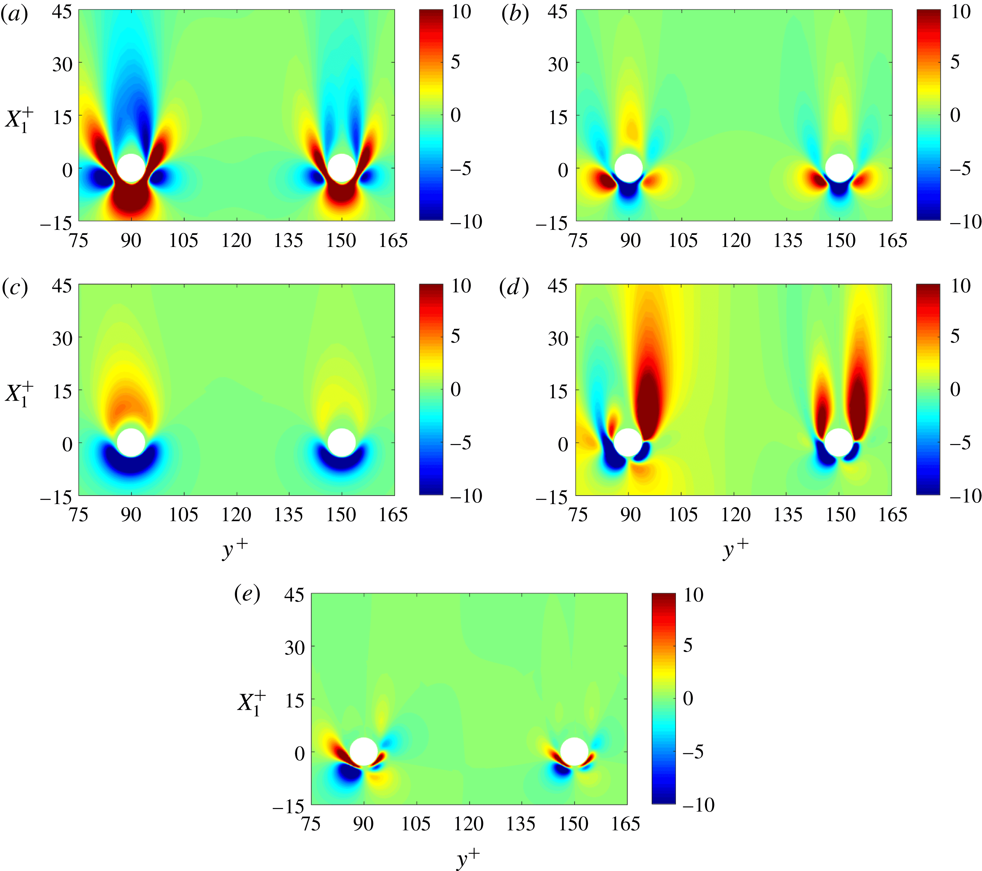
4.3 Turbulence production
The turbulence production term,
 $P_{\text{M}}$
, is positive everywhere in simple turbulent flows, but in this flow we see a region of strongly negative production near the front and the sides of each particle, and also a region of weakly negative production in the wake further away from the first particle. The region of negative production at the front has a thin neck, and before the flow reaches this neck it goes through a region with enhanced positive turbulence production. The decomposition of the production term is shown in figure 11. In this symmetry plane, there are five non-zero contributions to the production term:
 $-\unicode[STIX]{x1D619}_{\text{M}11}\langle \unicode[STIX]{x1D61A}_{11}\rangle _{\text{M}}$
,
 $-\unicode[STIX]{x1D619}_{\text{M}22}\langle \unicode[STIX]{x1D61A}_{22}\rangle _{\text{M}}$
,
 $-\unicode[STIX]{x1D619}_{\text{M}33}\langle \unicode[STIX]{x1D61A}_{33}\rangle _{\text{M}}$
,
 $-\unicode[STIX]{x1D619}_{\text{M}12}\unicode[STIX]{x2202}_{2}\langle u_{1}\rangle _{\text{M}}$
and
 $-\unicode[STIX]{x1D619}_{\text{M}12}\unicode[STIX]{x2202}_{1}\langle u_{2}\rangle _{\text{M}}$
.
Near the front of the particle, perpendicular to the particle surface, there is a nearly streamwise oriented axis where
 $\unicode[STIX]{x2202}_{2}\langle u_{1}\rangle _{\text{M}}+\unicode[STIX]{x2202}_{1}\langle u_{2}\rangle _{\text{M}}=0$
. Combining this with the approximation
 $\unicode[STIX]{x1D619}_{\text{M}22}\approx \unicode[STIX]{x1D619}_{\text{M}33}$
implying
 $b_{\text{M}22}\approx b_{\text{M}33}\approx -b_{\text{M}11}/2$
, the production on this axis is approximated by
 $$\begin{eqnarray}\displaystyle P_{\text{M}} & {\approx} & \displaystyle -\unicode[STIX]{x1D619}_{\text{M}11}\langle \unicode[STIX]{x1D61A}_{11}\rangle _{\text{M}}-\unicode[STIX]{x1D619}_{\text{M}22}\langle \unicode[STIX]{x1D61A}_{22}\rangle _{\text{M}}-\unicode[STIX]{x1D619}_{\text{M}33}\langle \unicode[STIX]{x1D61A}_{33}\rangle _{\text{M}}\nonumber\\ \displaystyle & = & \displaystyle -b_{\text{M}11}\langle \unicode[STIX]{x1D61A}_{11}\rangle _{\text{M}}-b_{\text{M}22}\langle \unicode[STIX]{x1D61A}_{22}\rangle _{\text{M}}-b_{\text{M}33}\langle \unicode[STIX]{x1D61A}_{33}\rangle _{\text{M}}\nonumber\\ \displaystyle & {\approx} & \displaystyle -b_{\text{M}11}(\langle \unicode[STIX]{x1D61A}_{11}\rangle _{\text{M}}+\langle \unicode[STIX]{x1D61A}_{22}\rangle _{\text{M}}/2+\langle \unicode[STIX]{x1D61A}_{33}\rangle _{\text{M}}/2)\nonumber\\ \displaystyle & = & \displaystyle -b_{\text{M}11}\langle \unicode[STIX]{x1D61A}_{11}\rangle _{\text{M}}/2.\end{eqnarray}$$
On this axis, the mean flow must decelerate (
 $\langle \unicode[STIX]{x1D61A}_{11}\rangle _{\text{M}}<0$
), which implies that
 $P_{\text{M}}$
has the same sign as the streamwise anisotropy
 $b_{\text{M}11}$
. Because of the anisotropy of the background turbulence
 $b_{\text{M}11}>0$
when the turbulence starts to approach the particle, and therefore the production is first enhanced in the deceleration zone. However, closer to the particle
 $b_{\text{M}11}$
becomes negative because the streamwise component is the normal component in the turbulent structure impinging on the front of the particle (see figure 8
d). As a consequence
 $P_{\text{M}}$
becomes strongly negative.
The regions of negative production at the sides of each particle are attributed to strongly positive
 $\unicode[STIX]{x1D619}_{\text{M}12}\unicode[STIX]{x2202}_{2}\langle u_{1}\rangle _{\text{M}}$
. To explain the positive correlation between
 $\unicode[STIX]{x1D619}_{\text{M}12}$
and
 $\unicode[STIX]{x2202}_{2}\langle u_{1}\rangle _{\text{M}}$
, we consider the region of negative
 $\unicode[STIX]{x1D619}_{\text{M}12}$
at the front-right side of the second particle: see figure 7(d). There is no perfect symmetry, but near the front there is an approximate symmetry about the axis
 $y^{+}=150$
. Near the particle surface and somewhat to the right of the symmetry line, there is a region where
 $\unicode[STIX]{x1D619}_{\text{M}12}>0$
(see figure 8
d),
 $\langle u_{1}\rangle _{\text{M}}$
increases with increasing
 $x_{2}$
(figure 8
a). Thus
 $\unicode[STIX]{x1D619}_{\text{M}12}\unicode[STIX]{x2202}_{2}\langle u_{1}\rangle _{\text{M}}>0$
and this provides a negative contribution to
 $P_{\text{M}}$
.
However, how can
 $\unicode[STIX]{x1D619}_{\text{M}12}$
become positive at this point? This cannot be due to the convection of the background
 $\unicode[STIX]{x1D619}_{\text{M}12}$
, because the background
 $\unicode[STIX]{x1D619}_{\text{M}12}$
is negative. To explain this, we choose a point near to the previous point, also on the
 $X_{3}=0$
plane, but closer to the approximate-symmetry axis, where
 $\unicode[STIX]{x1D619}_{\text{M}12}$
is rising or has just become positive. At this point we consider the turbulent structures with positive
 $u_{1}^{\prime \prime }$
, which tend to bend to the right, since
 $\langle u_{2}\rangle _{\text{M}}$
is slightly positive. The structures with positive
 $u_{1}^{\prime \prime }$
have relatively large inertia and therefore they will approach the particle very closely before they bend, so that
 $q^{\prime \prime }$
tends to be positive. After they have bent, their
 $u_{1}^{\prime \prime }$
and
 $u_{2}^{\prime \prime }$
are still relatively large, so that the fluctuating shear rate
 $\unicode[STIX]{x1D61A}_{12}^{\prime \prime }$
also tends to be positive. This implies a positive correlation of
 $q^{\prime \prime }$
and
 $\unicode[STIX]{x1D61A}_{12}^{\prime \prime }$
at this point, in other words a positive pressure term
 $\langle q^{\prime \prime }\unicode[STIX]{x1D61A}_{12}^{\prime \prime }\rangle _{\text{M}}$
, which appears in the transport equation of
 $\unicode[STIX]{x1D619}_{12}$
. If the correlation is sufficiently strong to overrule other mechanisms in that equation, for example negative production of
 $\unicode[STIX]{x1D619}_{\text{M}12}$
, then
 $\unicode[STIX]{x1D619}_{\text{M}12}$
becomes positive indeed.
In the wakes of both particles we see two wings of positive production, although the left wing in the wake of the first particle is relatively short. Each pair of wings (or in three dimensions each asymmetrically annular region of enhanced
 $P_{\text{M}}$
in the wake) corresponds to regions in an annular free shear layer where, as mentioned above,
 $\unicode[STIX]{x1D619}_{\text{M}12}$
and
 $\unicode[STIX]{x2202}_{2}\langle u_{1}\rangle$
have opposite signs, so that
 $-\unicode[STIX]{x1D619}_{\text{M}12}\unicode[STIX]{x2202}_{2}\langle u_{1}\rangle$
is positive and can enhance
 $P_{\text{M}}$
. In fact,
 $-\unicode[STIX]{x1D619}_{\text{M}12}\unicode[STIX]{x2202}_{2}\langle u_{1}\rangle$
appears in the production term of the
 $\unicode[STIX]{x1D619}_{\text{M}11}$
equation and not in those of the
 $\unicode[STIX]{x1D619}_{\text{M}22}$
and
 $\unicode[STIX]{x1D619}_{\text{M}33}$
equations. Furthermore, the wings of positive production at the right sides of the particles are stronger than those on the left. It seems that the right wings are responsible for the occurrence of maxima of
 $\unicode[STIX]{x1D619}_{\text{M}11}$
and large values of
 $b_{11}$
at
 $y^{+}\approx 100$
and
 $y^{+}\approx 160$
(see figure 8). If the particle Reynolds number based on the mean relative velocity were larger than a few hundred, then positive production in the wake would be expected since the particle wake would be unstable, for laminar free-stream flow and probably also for turbulent free-stream flow. However, in this case the particle Reynolds number remains moderate (maximum 50). Therefore, we do not attribute the positive
 $P_{\text{M}}$
in the wake to classical particle wake instability but to the interaction between the channel flow turbulence and the mean velocity gradients created by the particle.
Contours of moving-frame dissipation terms on the particle surface, viewed from a point on the polar axis (case T1). Turbulence dissipation rate
 $\unicode[STIX]{x1D716}_{\text{M}}$
on particles at
 $y^{+}=90$
(a) and
 $y^{+}=150$
(b). Mean flow dissipation rate
 $\unicode[STIX]{x1D701}_{\text{M}}$
on particles at
 $y^{+}=90$
(c) and
 $y^{+}=150$
(d).

4.4 Dissipation rates
The dissipation structure of kinetic energy near the particle is quantified by two quantities: the turbulence dissipation rate
 $\unicode[STIX]{x1D716}_{\text{M}}$
and the dissipation rate of mean flow kinetic energy, defined by
 $\unicode[STIX]{x1D701}_{\text{M}}=2\unicode[STIX]{x1D708}\langle \unicode[STIX]{x1D61A}_{ij}\rangle _{\text{M}}\langle \unicode[STIX]{x1D61A}_{ij}\rangle _{\text{M}}$
. The latter is not a term in the moving-frame TKE equation, but it is part of the fixed-frame turbulence dissipation rate, as we will see in § 5. The contours of
 $\unicode[STIX]{x1D716}_{\text{M}}$
and
 $\unicode[STIX]{x1D701}_{\text{M}}$
on the two particle surfaces, the entire hemispheres at one side of the symmetry plane
 $X_{3}=0$
, are shown in figure 12. The hemispheres appear as circles as we view the hemispheres along the polar axes, which are perpendicular to
 $X_{3}=0$
. Thus the centre of each circle shown corresponds to the point on the polar line
 $\unicode[STIX]{x1D703}=0$
at radius
 $r=r_{0}$
. Since the unladen
 $\unicode[STIX]{x1D716}_{\text{M}}$
is only 2.96 at
 $y^{+}=90$
and 1.17 at
 $y^{+}=150$
(see table 1), there are locations on the particle surface, in particular at the front and at the sides, where
 $\unicode[STIX]{x1D716}_{\text{M}}$
exceeds the unladen value by a factor of more than 100. However, the maximum of
 $\unicode[STIX]{x1D701}_{\text{M}}$
is even larger than
 $\unicode[STIX]{x1D716}_{\text{M}}$
, more than twice as large for
 $p=1$
, and more than eight times as large for
 $p=2$
(see table 4). Compared to the first particle, the turbulence around the second particle is weaker, so that the maximum of
 $\unicode[STIX]{x1D716}_{\text{M}}$
is lower, but the particle Reynolds number
 $Re_{p,tot}$
is larger (table 1), which leads to a larger maximum of
 $\unicode[STIX]{x1D701}_{\text{M}}$
.
Profiles of moving-frame statistics for particle
 $p=1$
from fine-grid simulation T1 (blue solid) and coarse-grid simulation T2 (red dashed). The turbulence dissipation rate
 $\unicode[STIX]{x1D716}_{\text{M}}$
(circles) and the mean flow dissipation rate
 $\unicode[STIX]{x1D701}_{\text{M}}$
(triangles) on three axes through the particle centre: the
 $x_{2}$
axis (a), the
 $x_{3}$
axis (b) and the
 $x_{1}$
axis (c). TKE budget terms divided by
 $\unicode[STIX]{x1D716}_{\text{M}}$
on the
 $x_{1}$
axis are shown in (d):
 $C_{\text{M}}/\unicode[STIX]{x1D716}_{\text{M}}$
(circles),
 $P_{\text{M}}/\unicode[STIX]{x1D716}_{\text{M}}$
(squares),
 $T_{\text{M}}/\unicode[STIX]{x1D716}_{\text{M}}$
(upward triangles),
 $\unicode[STIX]{x1D6F1}_{\text{M}}/\unicode[STIX]{x1D716}_{\text{M}}$
(diamonds) and
 $D_{\text{M}}/\unicode[STIX]{x1D716}_{\text{M}}$
(downward triangles); the inset zooms in on the region near the front of the particle.

At the channel walls,
 $\unicode[STIX]{x1D701}_{\text{M}}=\unicode[STIX]{x1D708}(\unicode[STIX]{x2202}_{2}\langle u_{1}\rangle _{\text{M}})^{2}$
. This is far away from particles, so that at
 $y^{+}=0$
,
 $\unicode[STIX]{x1D701}_{\text{M}}$
is virtually identical to the dissipation rate of the fixed-frame mean flow kinetic energy, defined by
 $$\begin{eqnarray}\displaystyle \unicode[STIX]{x1D701}=2\unicode[STIX]{x1D708}\langle \unicode[STIX]{x1D61A}_{ij}\rangle \langle \unicode[STIX]{x1D61A}_{ij}\rangle , & & \displaystyle\end{eqnarray}$$
and likewise the difference between
 $\unicode[STIX]{x1D716}_{\text{M}}$
and
 $\unicode[STIX]{x1D716}$
is negligible at the wall. Thus at the wall, we find
 $\unicode[STIX]{x1D701}_{\text{M}}\approx 176$
, approximately six times larger than
 $\unicode[STIX]{x1D716}_{\text{M}}$
at the wall. Thus also at that solid surface, the mean flow dissipation rate is much larger than the turbulence dissipation rate. It is possible to express the wall viscous length scale
 $\unicode[STIX]{x1D6FF}_{\unicode[STIX]{x1D708}}$
as a function of
 $\unicode[STIX]{x1D708}$
and the value of
 $\unicode[STIX]{x1D701}$
at the wall (
 $\unicode[STIX]{x1D701}_{w}$
):
 $\unicode[STIX]{x1D6FF}_{\unicode[STIX]{x1D708}}=(\unicode[STIX]{x1D708}^{3}/\unicode[STIX]{x1D701}_{w})^{1/4}$
. This expression is fully analogous to the expression for the Kolmogorov length scale, since the latter is obtained if
 $\unicode[STIX]{x1D701}_{w}$
is replaced by
 $\unicode[STIX]{x1D716}$
. It seems a logical step to also define a particle surface viscous length scale by
 $\unicode[STIX]{x1D6FF}_{\unicode[STIX]{x1D708},p}=(\unicode[STIX]{x1D708}^{3}/\unicode[STIX]{x1D701}_{\text{M}s})^{1/4}$
, where
 $\unicode[STIX]{x1D701}_{\text{M}s}$
denotes
 $\unicode[STIX]{x1D701}_{\text{M}}$
on the particle surface. This length scale depends on the position on the particle surface, and it is minimum at the location where
 $\unicode[STIX]{x1D701}_{\text{M}s}$
is maximum (a location on the surface of the second particle: see figure 12
d). This maximum is approximately 5000, so that the minimum
 $\unicode[STIX]{x1D6FF}_{\unicode[STIX]{x1D708},p}$
equals
 $0.44\unicode[STIX]{x1D6FF}_{\unicode[STIX]{x1D708},0}$
, which is larger than
 $0.26\unicode[STIX]{x1D6FF}_{\unicode[STIX]{x1D708},0}$
, the grid spacing at the particle surface in case T1. Thus, although
 $\unicode[STIX]{x1D701}_{\text{M}}$
attains very large values at the particle surface, the small length scale associated with
 $\unicode[STIX]{x1D701}_{\text{M}}$
is resolved in case T1.
Profiles of spherical surface averages of moving-frame statistics for particle
 $p=1$
from fine-grid simulation T1 (blue solid) and coarse-grid simulation T2 (red dashed). (a) The turbulence dissipation rate
 $\langle \unicode[STIX]{x1D716}_{\text{M}}\rangle _{\text{S}}$
(circles) and the mean flow dissipation rate
 $\langle \unicode[STIX]{x1D701}_{\text{M}}\rangle _{\text{S}}$
(triangles) as a function of
 $r^{+}$
(the distance to the particle). (b) TKE budget terms divided by
 $\langle \unicode[STIX]{x1D716}_{\text{M}}\rangle _{\text{S}}$
:
 $\langle C_{\text{M}}\rangle _{\text{S}}/\langle \unicode[STIX]{x1D716}_{\text{M}}\rangle _{\text{S}}$
(circles),
 $\langle P_{\text{M}}\rangle _{\text{S}}/\langle \unicode[STIX]{x1D716}_{\text{M}}\rangle _{\text{S}}$
(squares),
 $\langle T_{\text{M}}\rangle _{\text{S}}/\langle \unicode[STIX]{x1D716}_{\text{M}}\rangle _{\text{S}}$
(upward triangles),
 $\langle \unicode[STIX]{x1D6F1}_{\text{M}}\rangle _{\text{S}}/\langle \unicode[STIX]{x1D716}_{\text{M}}\rangle _{\text{S}}$
(diamonds) and
 $\langle D_{\text{M}}\rangle _{\text{S}}/\langle \unicode[STIX]{x1D716}_{\text{M}}\rangle _{\text{S}}$
(downward triangles).

Profiles of both dissipation rates on the three Cartesian axes through the centre of the first particle are shown in figure 13. These profiles consist of overlapping segments from the spherical and Cartesian grids. Figure 13(a–c) shows that
 $\unicode[STIX]{x1D701}_{\text{M}}$
decays faster than
 $\unicode[STIX]{x1D716}_{\text{M}}$
with increasing distance from the particle. Furthermore, figure 13(c) indicates that
 $\unicode[STIX]{x1D716}_{\text{M}}$
and
 $\unicode[STIX]{x1D701}_{\text{M}}$
are much lower in the wake than the maxima at the sides (figure 13
a,b), but also that in the wake the radii of the regions where
 $\unicode[STIX]{x1D716}_{\text{M}}$
and
 $\unicode[STIX]{x1D701}_{\text{M}}$
are elevated extend to relatively far away from the particle. Figure 13(d) illustrates that, locally, the absolute values of convection, turbulence production and pressure diffusion terms can be much larger than the turbulence dissipation rate.
To further quantify the effects of the moving-frame statistics, it is useful to reduce them to one-dimensional profiles. This can be done in several ways: one way to do this is illustrated in figure 14, another way is introduced in the next section. The spherical surface average
 $\langle \cdot \rangle _{\text{S}}$
reduces the 3-D statistics to profiles that are only a function of the distance to the particle centre. The operator denotes averaging over the surface of the sphere with radius
 $r$
and with the same centre as the particle. The spherical surface average of the TKE budget in the moving frame of the first particle is shown in figure 14(b), after division by
 $\langle \unicode[STIX]{x1D716}_{\text{M}}\rangle _{\text{S}}$
, which is shown in figure 14(a). Figure 14(b) looks somewhat similar to the radial budget shown in Vreman (Reference Vreman2016). In that paper, isotropic turbulence with zero mean flow over the particle was simulated, and apart from small effects of the cubical structure of the dilute array, the statistical variation in polar and azimuthal directions did not play a role there. This implied that there was no convection term. Furthermore, there was also no energy produced by shear, but the production was due to a stochastic forcing of the large scales. However, that production term did look similar to
 $\langle P_{\text{M}}\rangle _{\text{S}}$
shown in figure 14(b), while also the radial profiles of pressure diffusion and viscous transport were qualitatively similar to those shown in figure 14(b). In contrast, transport had a different shape: it was positive near the particle, in fact similar to
 $\langle C_{\text{M}}\rangle _{\text{S}}$
in the present case, while the present
 $\langle T_{\text{M}}\rangle _{\text{S}}$
is negative close to the particle. In figure 14(b), the dominant transport term is turbulent transport for
 $r^{+}>13.5$
, convection for
 $9.5<r^{+}<13.5$
, pressure diffusion for
 $5<r^{+}<9.5$
, and viscous diffusion for
 $r_{0}^{+}=4<r^{+}<5$
.
5 Fixed-frame averages of moving-frame statistics
It is important to realize that the fixed-frame average of a moving-frame statistical quantity, for example
 $\langle K_{\text{M}}\rangle$
, is in general different from the corresponding fixed-frame statistical quantity (
 $K$
in this example). In this section we apply the fixed-frame averaging operator to the 3-D moving-frame statistics from § 4, in order to compare these statistics, which characterize the true turbulence in this flow, to the unladen turbulence statistics.
The new findings in this section are: (i) large differences between the fixed-frame and moving-frame TKE budgets, (ii) the obscuring of the entire fixed-frame TKE budget and, to lesser extent, also the Reynolds stresses (mainly
 $\unicode[STIX]{x1D619}_{11}$
) by fluctuations that are steady in the moving frame, (iii) a net increase of production and dissipation of true turbulence in wall-parallel planes near the particles, although the particle Reynolds number is less than fifty, and (iv) a net increase of the dissipation of true turbulence in wall-parallel planes near the particles, albeit much smaller than the increase of the fixed-frame (fluid-weighted) turbulence dissipation rate.
In this section we denote an arbitrary fixed-frame statistical quantity by
 $Q$
and its moving-frame counterpart by
 $Q_{\text{M}}$
. The fixed-frame average of the moving-frame statistical quantity is equal to
 $\langle Q_{\text{M}}\rangle$
. The corresponding remainder is defined by
 $$\begin{eqnarray}\displaystyle Q_{R}=Q-\langle Q_{\text{M}}\rangle . & & \displaystyle\end{eqnarray}$$
It represents the contribution of the fluctuations that are steady in the moving frame to
 $Q$
. We thus obtain the decomposition
 $Q=\langle Q_{\text{M}}\rangle +Q_{R}$
. As mentioned in the Introduction, Risso et al. (Reference Risso, Roig, Amoura, Riboux and Billet2008) and Amoura et al. (Reference Amoura, Besnaci, Risso and Roig2017) decomposed the turbulence kinetic energy into two components via a decomposition of the velocity fluctuation. We apply the same decomposition to
 $f^{\prime }=f-\langle f\rangle$
, where
 $f$
represents a general fluid variable
 $f$
in the present flow configuration, and we define
 $$\begin{eqnarray}\displaystyle f^{\prime }=f^{\prime \prime }+f^{\prime \prime \prime },\quad f^{\prime \prime }=f-\langle f\rangle _{\text{M}},\quad f^{\prime \prime \prime }=\langle f\rangle _{\text{M}}-\langle f\rangle . & & \displaystyle\end{eqnarray}$$
Mathematical properties of combinations of fixed-frame and moving-frame averaging operators imply
 $\langle \langle u\rangle _{\text{M}}\rangle =\langle \boldsymbol{u}\rangle$
and
 $$\begin{eqnarray}\displaystyle \unicode[STIX]{x1D619}_{ij}-\langle \unicode[STIX]{x1D619}_{\text{M}ij}\rangle =\langle u_{i}^{\prime \prime \prime }u_{j}^{\prime \prime \prime }\rangle . & & \displaystyle\end{eqnarray}$$
This implies
 $$\begin{eqnarray}\displaystyle K_{R}=K-\langle K_{\text{M}}\rangle =\langle u_{i}^{\prime \prime \prime }u_{i}^{\prime \prime \prime }\rangle /2\geqslant 0. & & \displaystyle\end{eqnarray}$$
The decomposition
 $K=\langle K_{\text{M}}\rangle +K_{R}$
is precisely the decomposition used by Risso et al. (Reference Risso, Roig, Amoura, Riboux and Billet2008) and Amoura et al. (Reference Amoura, Besnaci, Risso and Roig2017). It is remarked that (5.3) can also be derived by application of the identity of Germano (Reference Germano1992).
Similarly, we can derive for the remainder of the turbulence dissipation rate:
 $$\begin{eqnarray}\displaystyle \unicode[STIX]{x1D716}_{R}=\unicode[STIX]{x1D716}-\langle \unicode[STIX]{x1D716}_{\text{M}}\rangle =2\unicode[STIX]{x1D708}\langle \unicode[STIX]{x1D61A}_{ij}^{\prime \prime \prime }\unicode[STIX]{x1D61A}_{ij}^{\prime \prime \prime }\rangle =2\unicode[STIX]{x1D708}\langle (\langle \unicode[STIX]{x1D61A}_{ij}\rangle _{\text{M}}-\langle \unicode[STIX]{x1D61A}_{ij}\rangle )^{2}\rangle =\langle \unicode[STIX]{x1D701}_{\text{M}}\rangle -\unicode[STIX]{x1D701}\geqslant 0. & & \displaystyle\end{eqnarray}$$
Thus
 $K_{R}$
and
 $\unicode[STIX]{x1D716}_{R}$
are the kinetic energy and the dissipation rate based on
 $\boldsymbol{u}^{\prime \prime \prime }$
. In fact, we can decompose the entire fixed-frame TKE budget (
 $C+P+T+\unicode[STIX]{x1D6F1}+D-\unicode[STIX]{x1D716}+I+B=0$
) into two TKE budgets. This is shown in appendix E, where it is also mathematically proved that the interfacial term in the fixed-frame budget is entirely due to fluctuations that are steady in the moving frame (if
 $u_{i}^{p}$
does not depend on time).
Fixed-frame averages of moving-frame budget terms
 $\langle Q_{\text{M}}\rangle$
(thick black solid) from T1 compared with the unladen counterparts from T0 (thin black dash-dotted) and with the fixed-frame counterparts
 $Q$
(thin blue solid) from T1. (a)
 $Q=K$
, (b)
 $Q=\unicode[STIX]{x1D619}_{11}$
, (c)
 $Q=\unicode[STIX]{x1D619}_{22}$
(squares) and
 $Q=\unicode[STIX]{x1D619}_{33}$
(triangles) and (d)
 $Q=\unicode[STIX]{x1D619}_{12}$
.

Results of the TKE and the Reynolds stresses are shown in figure 15. Near the particle locations,
 $\langle K_{\text{M}}\rangle$
appears to be substantially lower than the result shown in § 3, included as a thin blue line in figure 15(a). We can now conclude that the surprising bump at
 $y^{+}=150$
in the fixed-frame TKE is entirely due to structures that are steady in the moving frame, structures due to the displacement of liquid by particles which have non-zero mean relative velocity. The kinetic energy of the true turbulence,
 $\langle K_{\text{M}}\rangle$
, displays a valley at
 $y^{+}=150$
. This means that the attenuation of true turbulence is relatively strong at the particle locations, in contrast to the impression raised by the profile of the complete
 $K$
(see figure 2). Furthermore, figure 15(b–d) shows that the fluctuations that are steady in the moving frame are concentrated in the streamwise velocity component (
 $\langle \unicode[STIX]{x1D619}_{\text{M}22}\rangle \approx \unicode[STIX]{x1D619}_{22}$
and
 $\langle \unicode[STIX]{x1D619}_{\text{M}33}\rangle \approx \unicode[STIX]{x1D619}_{33}$
), which is in line with the results of the experiments by Amoura et al. (Reference Amoura, Besnaci, Risso and Roig2017).
Fixed-frame averages of moving-frame statistics
 $\langle Q_{\text{M}}\rangle$
(thick black solid) from T1 compared with the unladen counterparts from T0 (thin black dash-dotted) and with the fixed-frame counterparts
 $Q$
(thin blue solid). (a)
 $Q=P$
, (b)
 $Q=T$
, (c)
 $Q=\unicode[STIX]{x1D6F1}$
(squares), (d)
 $Q=D$
(circles), (e)
 $Q=-\unicode[STIX]{x1D716}$
. Also in (b)
 $\langle C_{\text{M}}\rangle$
from T1 (dotted). Also in (e) the remainder
 $-\unicode[STIX]{x1D716}_{R}=-(\unicode[STIX]{x1D716}-\langle \unicode[STIX]{x1D716}_{\text{M}}\rangle )$
(thin red solid) and
 $\langle \unicode[STIX]{x1D701}_{\text{M}}\rangle$
(thin red dashed). (f) Zoom of two curves of (e),
 $-\langle \unicode[STIX]{x1D716}_{\text{M}}\rangle$
from T1 (thick black solid) and
 $-\unicode[STIX]{x1D716}$
from T0 (thin black dash-dotted). Also in (f) the budget error,
 $\langle E_{\text{M}}\rangle$
(black dotted), from T1.

The fixed-frame averages of the terms in the moving-frame budget are shown in figure 16 (like
 $B$
,
 $\langle B_{\text{M}}\rangle$
is negligible and not shown). There are two peaks in
 $\langle P_{\text{M}}\rangle$
somewhat to the right of each particle location (figure 16
a). These peaks are due to the relatively large production at several locations around the particle, in particular in the wake (see figure 10
b). The shift to the right can be due to the asymmetry in the two wings in the wake. The asymmetry is due to inhomogeneity in the wall-normal direction. In addition, the background production is decaying with increasing distance of the wall. Thus even a symmetric addition to the production results in a production peak that is somewhat shifted to the right. The convection term
 $\langle C_{\text{M}}\rangle$
is not shown in a separate plot, but in the plot of the transport term, because after the planar averaging, the term has become relatively small, while the fixed-frame counterpart
 $C$
is equal to zero. The profiles of the averages of the moving-frame pressure diffusion and viscous diffusion are much smoother and smaller than their fixed-frame counterparts
 $\unicode[STIX]{x1D6F1}$
and
 $D$
.
The most striking observation in figure 16 is that
 $\langle \unicode[STIX]{x1D716}_{\text{M}}\rangle$
is much smaller than
 $\unicode[STIX]{x1D716}$
, near the particle locations. In these regions, the contribution due to fluctuations that are steady in the moving frame,
 $\unicode[STIX]{x1D716}_{R}=\unicode[STIX]{x1D716}-\langle \unicode[STIX]{x1D716}_{\text{M}}\rangle$
, turns out to be larger than the contribution due to fluctuations that are unsteady in the moving frame, in particular for the second particle. Equation (5.5) and the fact that
 $\unicode[STIX]{x1D701}$
is only large near the wall imply that
 $\unicode[STIX]{x1D716}_{R}\approx \langle \unicode[STIX]{x1D701}_{\text{M}}\rangle$
in the core of the channel, which is confirmed by figure 16(e). More details of the profile of
 $\langle \unicode[STIX]{x1D716}_{\text{M}}\rangle$
are shown in figure 16(f). Although
 $\langle \unicode[STIX]{x1D716}_{\text{M}}\rangle$
is much smaller than
 $\unicode[STIX]{x1D716}$
, the sole contribution of the fluctuations that are unsteady in the moving frame appears to be significantly larger than the unladen turbulence dissipation rate in small regions (slightly wider than
 $d_{p}$
) around the positions of the particle centres. Further away from the particles, the turbulence dissipation rate is significantly suppressed.
Whereas the results of the laminar case in § 3.2 (figure 6) only suggested that the remarkable local maximum of the fixed-frame
 $K$
at
 $y^{+}=150$
(figure 2) and the strong enhancement of the fixed-frame
 $\unicode[STIX]{x1D716}$
are not entirely due to true turbulence, figure 15 proves that this maximum is caused by (streamwise velocity) fluctuations that are steady in the moving frame, while figure 16(e) and equation (5.5) prove that the very strong enhancement of the fixed-frame dissipation rate around the particles is mostly due to the dissipation of the kinetic energy of the mean flow.
Zonal averages of statistics of case T0 and fixed-frame (T1) and moving-frame (T1M) statistics from case T1 (
 $TT=C+T+\unicode[STIX]{x1D6F1}+D$
is the total transport, and
 $b_{11}$
is the streamwise anisotropy coefficient based on zonal averages of Reynolds stresses).

We finish this section with the presentation of table 5, in which the overall effects of the particles on the statistics are quantified. The entire channel half has been split into three subregions with a width of 60 unladen wall units each
 $0\leqslant y^{+}\leqslant 60$
(zone 1),
 $60\leqslant y^{+}\leqslant 120$
(zone 2),
 $120\leqslant y^{+}\leqslant 180$
(zone 3). The entire channel half is called zone 4. For each zone, the zonal average of a statistical quantity
 $f$
is defined by the integral of
 $\unicode[STIX]{x1D6FC}f$
over the volume of the zone divided by the integral of
 $\unicode[STIX]{x1D6FC}$
over the volume of the zone. The statistics of the true turbulence (Reynolds stresses, TKE, turbulence production and turbulence dissipation rate in the moving frame) are all significantly attenuated, in all zones. The overall attenuation of the TKE increases with increasing distance from the wall. The global attenuation (zone 4) of the turbulence kinetic energy (20 %) is higher than that of the turbulence dissipation rate (14 %), which suggests that large scales are attenuated more than small scales. However, the fixed-frame turbulence dissipation rate is globally enhanced by (2 %), but this enhancement is not due to true turbulence but to fluctuations that are steady in the moving frame, the fluctuations produced by the interfacial term
 $I$
, which is solely due to mechanisms at the interfacial surface and accounts for
 $17\,\%$
of the total production in the fixed frame.
For flows in which the turbulence is attenuated, an increase of the overall
 $\unicode[STIX]{x1D716}$
by the particles is unexpected; point-particle simulations of particle-laden turbulent channel flow resulted in a reduction of the overall turbulence dissipation rate (Vreman Reference Vreman2015). In the TKE equation of the point-particle approach, there are two dissipative terms: the resolved turbulence dissipation rate and the particle-induced dissipation. The sum of these two terms acts as a model for the present
 $\unicode[STIX]{x1D716}-I$
in the fixed frame. The global
 $\unicode[STIX]{x1D716}-I$
(zone 4) is equal to
 $P$
, which is reduced. With respect to comparison between fixed-frame and moving-frame statistics, we observe that the overall differences are small for the Reynolds stresses, but large for the production and turbulence dissipation rate (in zones 2, 3 and 4). The last line in table 5 shows that the anisotropy of the turbulence is significantly enhanced in all zones.
6 Turbulence attenuation and increased anisotropy
In the previous sections we observed that the TKE is attenuated and the anisotropy of the turbulence is increased by the particles. It is tempting to attribute at least the turbulence attenuation to the very strong increase of the turbulence dissipation rate near the particles. However, we need to be cautious. The previous section showed that not only is the (moving-frame) turbulence dissipation rate increased near particles (figure 16 f) but that the production is also increased, at least in some wall-parallel planes (see figure 16 a). It is therefore not clear why, compared to the unladen flow, the TKE is reduced everywhere. Furthermore, is it possible to explain from changes in the terms in the TKE budget, which is a TKE balance, the attenuation of the TKE? And which feature of the flow is causing the increase of turbulence anisotropy? In this section, we address these questions in further detail. For this purpose, we evaluate (1) spectra of the individual velocity components, (2) turbulence kinetic energy transfer towards the particles, (3) the effect of non-uniform streamwise forcing of the flow.
The new findings in this section are: (i) the attenuation of all spatial scales far away from the particles, (ii) an enhancement of small spatial scales closer to the particles, predominantly in the streamwise velocity, (iii) local occurrences of counter-gradient diffusion, which are caused by the particles, (iv) the observation of radial transport of turbulence kinetic energy towards particles embedded in a turbulent channel flow and (v) that non-uniform mean flow forcing can explain most of the turbulence attenuation and anisotropy increase observed in a PR-DNS of a turbulent channel flow laden with a small volume fraction of particles with large Stokes response time.
A Fourier spectral analysis of the fluid motion in particle-laden flows is not straightforward. If the velocity inside the particles is used in the Fourier transform, then the discontinuity of the velocity derivatives on the particle surfaces affects the spectra; the discontinuity is expected to produce
 $k^{-4}$
fall-off for
 $k\rightarrow \infty$
(
 $k$
is the wavenumber). In this flow, we are fortunately able to define periodic lines which do not cut through any solid boundary. Spanwise spectra on two of such lines are shown in figure 17. The first line lies on the plane
 $y^{+}=150$
and cuts through the wake of particle
 $p=2$
, the second lies on the centre plane. The spectra are based on the velocity fluctuations in the moving frame. The unladen flow spectra shown were produced by the high-resolution spectral simulation S4-B3 (Vreman & Kuerten Reference Vreman and Kuerten2016), which had even higher resolution than simulation S2 (Vreman & Kuerten Reference Vreman and Kuerten2014).
Spanwise one-dimensional velocity spectra on the line defined by
 $y^{+}=150$
and
 $X_{1}^{+}=16$
(a,b) and the line defined by
 $y^{+}=180$
and
 $X_{1}^{+}=16$
(c,d), based on the moving-frame fluctuations of
 $u_{1}$
(blue, circle),
 $u_{2}$
(red) and
 $u_{3}$
(black). The solid and dashed lines in (a,c) represent T1 and T0, respectively. Spectra divided by the unladen counterparts are shown in (b,d).

Figure 17(a,b) shows an attenuation of large scales and an enhancement of small scales. In the streamwise velocity fluctuation, the enhancement of small scales is much larger than in the other two velocity fluctuations. On the first periodic line, the contribution of the small scales (
 $k\geqslant 23$
, on the right of the circle in figure 17
b) to the streamwise velocity fluctuation is approximately 10 %, while these scales only contribute
 $1\,\%$
to the other two components. Since the large scales in the wall-normal velocity component appear to be attenuated less than those in the streamwise velocity, the streamwise anisotropy on this line is not enhanced despite the relatively large increase of small scales in the streamwise velocity fluctuations. Furthermore, the enhancement of small scales is restricted to locations near the particles: on the periodic line in the centre plane all scales are attenuated (figure 17
c,d). In fact, an attenuation of all scales in each velocity components has been found in most planes parallel to the wall and reasonably far away from the particles, for example also in the plane
 $y^{+}=120$
and in the planes in the near-wall region (
 $y^{+}\leqslant 60$
). Thus the spectral analysis shows the attenuation of the distinct scales, but it does not reveal the main cause of the observed global attenuation of turbulence and increase of turbulence anisotropy.
In flows with zero (or low) particle velocity fluctuation, the no-slip condition on the particle surface suppresses
 $\boldsymbol{u}^{\prime \prime }$
and thereby
 $K_{\text{M}}$
on the particle surface. Since the velocity is continuous, a region of low
 $K_{\text{M}}$
is created in the neighbourhood of the particle. Since the volume fraction of all low-
 $K_{\text{M}}$
regions surrounding the particles may be significant, this argument can be used to explain part of the overall turbulence attenuation, but only if there are no mechanisms by which the particles can generate new
 $K_{\text{M}}$
. However, the particles do generate new
 $K_{\text{M}}$
, at least in some regions. The generation of new
 $K_{\text{M}}$
is part of the moving-frame TKE budget, which can be written as
 $$\begin{eqnarray}\displaystyle \langle u_{j}\rangle _{\text{M}}\unicode[STIX]{x2202}_{j}K_{\text{M}}=-\unicode[STIX]{x2202}_{j}\unicode[STIX]{x1D709}_{j}+P_{\text{M}}-\unicode[STIX]{x1D716}_{\text{M}}, & & \displaystyle\end{eqnarray}$$
where
 $\unicode[STIX]{x1D743}$
is the diffusive flux vector such that
 $T_{\text{M}}+\unicode[STIX]{x1D6F1}_{\text{M}}+D_{\text{M}}=-\unicode[STIX]{x2202}_{j}\unicode[STIX]{x1D709}_{j}$
. We call
 $P_{\text{M}}-\unicode[STIX]{x1D716}_{\text{M}}$
the net source term. Positive and negative values of this term correspond to net injection and net destruction of turbulence kinetic energy, respectively. Figure 18(a) illustrates that each particle creates two regions of net injection of
 $K_{\text{M}}$
, two regions where the production exceeds the dissipation: an asymmetric annular region in the wake and a ball-shaped region upstream of the particle. If the diffusive term were negligible, equation (6.1) would imply an increase or decrease of
 $K_{\text{M}}$
in the direction of the mean velocity vector if
 $P_{\text{M}}-\unicode[STIX]{x1D716}_{\text{M}}$
is positive or negative, respectively.
The quantities
 $P_{\text{M}}-\unicode[STIX]{x1D716}_{\text{M}}$
(a) and
 $-\unicode[STIX]{x1D709}_{j}\unicode[STIX]{x2202}_{j}K_{\text{M}}$
(b) in the plane
 $X_{3}=0$
(case T1). Contours have been clipped to the range
 $[-10,10]$
. The dashed demarcation lines illustrate a subdivision of zones 1, 2 and 3 into zones 1a, 1b, 2a, 2b, 3a and 3b. The regions enclosed by the solid black contours in (b) correspond to
 $-\unicode[STIX]{x1D709}_{j}\unicode[STIX]{x2202}_{j}K_{\text{M}}\leqslant -0.1$
.

More formally, equation (6.1) supplied with periodic or homogenenous Dirichlet boundary conditions for
 $K_{\text{M}}$
implies
 $$\begin{eqnarray}\displaystyle \int _{\unicode[STIX]{x1D6FA}}(P_{\text{M}}-\unicode[STIX]{x1D716}_{\text{M}})K_{\text{M}}\,\text{d}\unicode[STIX]{x1D6FA}=-\int _{\unicode[STIX]{x1D6FA}}\unicode[STIX]{x1D709}_{j}\unicode[STIX]{x2202}_{j}K_{\text{M}}\,\text{d}\unicode[STIX]{x1D6FA}. & & \displaystyle\end{eqnarray}$$
If this integral is positive then
 $K_{\text{M}}$
and
 $P_{\text{M}}-\unicode[STIX]{x1D716}_{\text{M}}$
are positively correlated:
 $K_{\text{M}}$
tends to be low if
 $P_{\text{M}}-\unicode[STIX]{x1D716}_{\text{M}}<0$
and high if
 $P_{\text{M}}-\unicode[STIX]{x1D716}_{\text{M}}>0$
(note that the domain integral of
 $P_{\text{M}}-\unicode[STIX]{x1D716}_{\text{M}}$
must be zero). Figure 18(b) shows that
 $-\unicode[STIX]{x1D709}_{j}\unicode[STIX]{x2202}_{j}K_{\text{M}}$
is predominantly positive, although regions with counter-gradient diffusion (negative
 $-\unicode[STIX]{x1D709}_{j}\unicode[STIX]{x2202}_{j}K_{\text{M}}$
) occur. If we assume a standard model expression for the diffusive flux,
 $\unicode[STIX]{x1D709}_{j}=-\unicode[STIX]{x1D708}_{t}\unicode[STIX]{x2202}_{j}K_{\text{M}}$
with a positive turbulence diffusivity
 $\unicode[STIX]{x1D708}_{t}$
, then the correlation expressed by (6.2) is ensured to be positive. Furthermore, a positive
 $\unicode[STIX]{x1D708}_{t}$
implies that each local minimum (maximum) of
 $K_{\text{M}}$
occurs in a region of negative (positive)
 $P_{\text{M}}-\unicode[STIX]{x1D716}_{\text{M}}$
(if
 $K_{\text{M}}$
attains a local minimum, then
 $\unicode[STIX]{x2202}_{j}K_{\text{M}}=0$
and
 $\unicode[STIX]{x2202}_{j}^{2}K_{\text{M}}>0$
so that (6.1) implies that
 $P_{\text{M}}-\unicode[STIX]{x1D716}_{\text{M}}<0$
). Indeed, the particle surface, which corresponds to minimum
 $K_{\text{M}}$
, is enclosed by a region of strongly negative
 $P_{\text{M}}-\unicode[STIX]{x1D716}_{\text{M}}$
, which can only be maintained if it is balanced by transport of
 $K_{\text{M}}$
into this region from further away.
Fixed-frame averages of moving-frame wall-normal energy fluxes per unit channel wall surface area (a) and spherical surface averages for
 $p=1$
(b) and
 $p=2$
(c) of moving-frame radial energy fluxes per unit channel wall surface area: convective transport (circles), turbulent transport (upward triangles), pressure diffusion (diamonds), viscous diffusion (downward triangles) and total flux (black solid) of case T1 and total flux of case T0 (dash-dotted). (d) Spherical surface average of
 $K_{\text{M}}$
(no symbols) and the anisotropy coefficient
 $b_{11,\text{S}}=-1+3\langle \unicode[STIX]{x1D619}_{\text{M}11}\rangle _{\text{S}}/2\langle K_{\text{M}}\rangle _{\text{S}}$
(symbols) for
 $p=1$
(solid lines) and
 $p=2$
(dashed lines).

Furthermore, the profiles of the energy fluxes averaged over certain directions also indicate that the particles draw TKE from their surroundings (figure 19). Figure 19(a) shows averaged wall-normal components of the statistics inside the divergences of the four transport terms: the convection flux
 $\langle \langle u_{2}\rangle _{\text{M}}K_{\text{M}}\rangle$
, the turbulent transport flux
 $\langle \langle u_{i}^{\prime \prime }u_{i}^{\prime \prime }u_{2}^{\prime \prime }\rangle _{\text{M}}\rangle /2$
, the pressure diffusion flux
 $\langle \langle q^{\prime \prime }u_{2}^{\prime \prime }\rangle _{\text{M}}\rangle$
and the viscous diffusion flux
 $-2\unicode[STIX]{x1D708}\langle \langle u_{j}^{\prime \prime }\unicode[STIX]{x1D61A}_{2j}^{\prime \prime }\rangle _{\text{M}}\rangle$
. The total wall-normal transport flux, which is directed towards the channel centre, drops faster near the particle locations since part of the wall-normal flow of energy is drawn towards the particles. However, somewhat later the wall-normal flux recovers, because the particles also generate new
 $K_{\text{M}}$
through positive
 $P_{\text{M}}-\unicode[STIX]{x1D716}_{\text{M}}$
. Analogously defined radial fluxes averaged over spherical surfaces around the particle centre are shown in figure 19(b,c) (after multiplication with
 $4\unicode[STIX]{x03C0}r^{2}\cdot 436/(4\unicode[STIX]{x03C0}\cdot 4\unicode[STIX]{x03C0}/3)$
to obtain the energy transfer to all particles of type
 $p$
per unit surface area of the channel wall; the corresponding total radial energy fluxes of the unladen flow, which are entirely due to wall-normal inhomogeneity, are shown too). Negative values denote a radial flux of energy towards the particles. The pressure diffusion flux plays a very important role in the radial transport of TKE: it is the dominant energy flux for
 $5<r^{+}<25$
if
 $p=1$
and
 $5<r^{+}<20$
if
 $p=2$
. Convection is also important over a large range of radii if
 $p=1$
.
Although the turbulence shows a clear dependence on the radius close to the particles (figure 19
d), with increasing radius the TKE and the anisotropy coefficients display a rather rapid approach to the corresponding zonal averaged values tabulated in § 5 (zones 2 and 3 correspond to
 $p=1$
and
 $p=2$
, respectively), more rapid than we had expected in view of the strong overall turbulence attenuation and increase of anisotropy. The question arises whether the overall turbulence attenuation and significant change of anisotropy in the entire channel (also in the particle-free regions near the channel walls) are entirely caused by the observed fluxes of TKE towards the particles.
Zonal averages of moving-frame statistics from case T1. The ratios to the unladen counterparts are shown in brackets.
 $TT=C+T+\unicode[STIX]{x1D6F1}+D$
denotes the total transport, and
 $b_{11}$
denotes the streamwise anisotropy coefficient based on zonal averages of Reynolds stresses.

In fact, the same question arises from the following comparison between regions with and regions without particles. We partition each main zone (1, 2 and 3) into two smaller zones with equal volumes (zones 1a, 1b, 2a, 2b, 3a and 3b), as illustrated by the demarcation lines in figure 18(b). Zones 2a and 3a contain particles, while the other zones contain no particles. Zones of type a correspond to the region
 $-15.7<X_{1}^{+}\leqslant 47.1$
of the reference block, while zones of type b correspond to
 $-31.4<X_{1}^{+}\leqslant -15.7$
or
 $47.1<X_{1}^{+}\leqslant 94.2$
. Although the partitioning is defined such that the elongated regions of visually reduced TKE (figure 8
a) reside almost entirely inside zones 2a and 3a, both the TKE and the anisotropy coefficient in zones 2a and 3a are hardly different from those in zones 2b and 3b, as shown in table 6. We do see that the production and dissipation in zone 2a (3a) are both significantly larger than in zone 2b (3b). Since for the dissipation this effect is stronger than for the production, the net total transport of energy into zone 2a (3a) is larger than into zone 2b (3b). This indicates that there is a net flow of energy from zone 2b (3b) into zone 2a (3a). From direct computation of the total transport flux across zonal boundaries, we found that the net flow of energy per unit volume from zone 2b (3b) to zone 2a (3a) is 0.26 (0.074), which appears to be approximately equal to half the difference between the averaged transport terms of zones 2a and 2b (3a and 3b). Thus the loss of energy of zone 2b to zone 2a is approximately 11 % of the dissipation of zone 2b (which is equal to the total energy input in the zone 2b), while the loss of energy of zone 3b to zone 3a is approximately 8 % of the dissipation of zone 3b. However, compared to the unladen flow the dissipation is reduced much more, by 25 % in zone 2b and 32 % in zone 3b, while the corresponding relative reductions of the production and TKE are even larger.
Statistics of T5 (blue dashed, the unladen simulation with non-uniform mean driving force) compared with fixed-frame averages of moving-frame statistics of T1 (thick solid) and statistics of T0 (thin black dash-dotted, the reference unladen simulation). (a) Mean velocity, (b) Reynolds shear stress, (c) streamwise diagonal Reynolds stress, (d) wall-normal diagonal Reynolds stress, (e) spanwise diagonal Reynolds stress, (f) streamwise and wall-normal anisotropy coefficients,
 $b_{11}=-1+3\langle \unicode[STIX]{x1D619}_{\text{M}11}\rangle /\langle 2K_{\text{M}}\rangle$
(positive) and
 $b_{22}=-1+3\langle \unicode[STIX]{x1D619}_{\text{M}22}\rangle /\langle 2K_{\text{M}}\rangle$
(negative), respectively.

Finally, in order to find a more complete explanation of the observed attenuation and increase of anisotropy, we move on to explore the effect of non-uniform streamwise forcing caused by the presence of the particles. Research based on point-particle simulations with freely moving heavy particles has shown that turbulence attenuation in particle-laden channel flows can be caused by two different effects (Vreman Reference Vreman2015): the direct effect of the particles on the turbulence kinetic energy and the non-uniformity of the mean particle force, which is a direct effect of the particles on the mean momentum. The question arises whether similar conclusions on turbulence attenuation can be drawn from the particle-resolved simulation of this idealized flow. Let us therefore define a piecewise constant average force density vector
 $\boldsymbol{f}=(f_{1},0,0)$
, where
 $f_{1}$
is equal to zero in zone 1 (
 $0\leqslant y^{+}\leqslant 60$
),
 $-0.401$
in zone 2 (
 $60\leqslant y^{+}\leqslant 120$
) and
 $-0.627$
in zone 3 (
 $120\leqslant y^{+}180$
). The values in zones 2 and 3 are the mean particle forces in table 3 multiplied by the number of particles and divided by the volume of each zone. In addition to T0, we perform another simulation of turbulent channel flow without particles, simulation T5, in which the uniform driving force
 $\boldsymbol{a}$
is replaced by the non-uniform driving force
 $\boldsymbol{a}+\boldsymbol{f}$
, while
 $\boldsymbol{a}=(a_{1},0,0)$
is a spatially constant acceleration vector, adjusted in time to keep the bulk velocity constant and the same as in the unladen case. The non-uniform driving force is non-uniform in the wall-normal direction only. Compared to the unladen case, this driving force has an accelerating effect in the near-wall region (zone 1) and a decelerating effect in the other zones (in zone 3 more than in zone 2).
Figure 20 shows that this simple modification of the mean driving force in an otherwise unladen channel flow is able to reproduce a large part of the attenuation of the turbulence and the increase of anisotropy in the particle-resolved simulation. It is stressed that there is no temporal fluctuation in
 $\boldsymbol{f}$
, so that no term with
 $\boldsymbol{f}$
occurs in the turbulence kinetic energy equation. It is the overall structure of the turbulence that changes; physical instability mechanisms leading to turbulence are modified by non-uniformity of the driving force, as can be inferred from a linear stability analysis (Vreman Reference Vreman2015). The mean velocity profile remains approximately the same so that the non-uniformity of the mean forcing is compensated by a change of the Reynolds shear stress in the mean momentum equation, a change that implies a reduction of the Reynolds shear stress (and the TKE): see Vreman (Reference Vreman2015). For completeness we mention that the friction velocity
 $u_{\unicode[STIX]{x1D70F}}$
in case T5 was equal to 0.98, the same as in case T1, and nearly equal to one (
 $u_{\unicode[STIX]{x1D70F},0}$
).
Most, but not all, turbulence attenuation in case T1 is reproduced by T5 (figure 20). Since T5 reproduces the turbulence attenuation better in the zones without particles (zone 1) than in the zones with particles (zones 2 and 3), we attribute the rest of the turbulence attenuation to local effects: particles create strong sinks of turbulence kinetic energy near their surfaces and draw turbulence kinetic energy from their surroundings via the transport terms, for which the pressure diffusion term is surprisingly relevant.
7 Conclusions
We considered turbulent channel flow past a moving array of spherical particles, for a particle size of
 $d_{p}^{+}=8$
and an overall particle volume fraction of 0.00075. In order to achieve a sharp representation of the particle interfaces, the flow was simulated by means of an overset grid method, using spherical grids around each particle overset on a background Cartesian grid. In order to achieve an acceptable computation time without compromising the accuracy of the Navier–Stokes solution near the surfaces of the rather small particles, no particles were located near the channel walls. We observed that the turbulence kinetic energy (TKE) was significantly attenuated by the particles, also in the particle-free regions. Furthermore, the relative attenuation of the wall-normal and spanwise velocity fluctuations was larger than for the streamwise velocity fluctuations so that the anisotropy of the turbulence increased. These findings are consistent with previous observations from experiments and point-particle simulations of dilute vertical gas–solid flow at high Stokes number and low particle volume fraction in the literature.
An important aim of this paper was to investigate the budget of the attenuated TKE in detail, the 1-D budget in the fixed frame of the channel (§ 3) and the 3-D budget in the moving frame of the particles (§ 4). The moving-frame analysis allowed us to extract the fluctuations solely due to true turbulence and to reveal and explore the rich structure of the 3-D turbulence inhomogeneity produced by the particles. By applying the fixed-frame averaging operator to the 3-D moving-frame results, both types of statistics could be compared to each other and the cause of the discrepancies could be explained (§ 5). Physical explanations for the turbulence attenuation and increase of anisotropy were addressed in § 6, in which a brief spectral analysis of the individual velocity components was included. The main new findings of §§ 2–6 have been summarized in the second paragraph of each section and are not repeated here.
Whereas the investigated turbulent channel flow past an array of spheres moving with constant velocity is a neat and well-defined flow case, it is also a specialized case whose results depend on the parameter settings. For example, if the particle volume fraction is reduced while particle diameter and array velocity remain the same, then the turbulence will be attenuated less and somewhat higher peak values of the 3-D budget terms near the particles will occur. If the particle diameter is reduced while particle volume fraction and array velocity remain the same, the turbulence will be attenuated more. Provided the turbulence remains sufficiently strong, the smaller particle diameter will cause an increase of the maximum of the 3-D turbulence dissipation rate attained on the particle surface. For other particle shapes under otherwise comparable flow conditions, main features of the turbulence statistics, such as global attenuation of the turbulence kinetic energy, strong enhancement of the dissipation rates near the particle surface and negative turbulence production in front of the particle, are expected to be similar as for spherical particles.
Acknowledgements
This work was sponsored by NWO Exacte en Natuurwetenschappen (Physical Sciences) for the use of supercomputer facilities, with financial support from the Nederlandse Organisatie voor Wetenschappelijk Onderzoek (Netherlands Organization for Scientific Research, NWO).
Appendix A. The generalized fixed-frame TKE equation
Let us consider a general multiphase fluid of
 $N$
phases in domain
 $\unicode[STIX]{x1D6FA}_{0}$
. We follow the standard approach and define for each phase
 $k$
the so-called indicator function
 $\unicode[STIX]{x1D712}_{k}$
, which depends on location
 $\boldsymbol{x}$
and time
 $t$
and equals
 $1$
if phase
 $k$
is present at
 $(\boldsymbol{x},t)$
and 0 otherwise. At each
 $(\boldsymbol{x},t)$
precisely one component is present, which implies that for all
 $(\boldsymbol{x},t)$
the sum of all
 $\unicode[STIX]{x1D712}_{k}$
equals 1. Furthermore, for all
 $(\boldsymbol{x},t)$
the density
 $\unicode[STIX]{x1D70C}$
, each velocity component
 $u_{i}$
, each stress component
 $\unicode[STIX]{x1D70C}\unicode[STIX]{x1D70E}_{ij}$
and each body-force component
 $\unicode[STIX]{x1D70C}a_{i}$
are equal to those for component phase
 $k$
if
 $\unicode[STIX]{x1D712}_{k}=1$
. The flow variables may be discontinuous at interfaces, in particular the density. Also the density within a given phase may be variable; this generality does not complicate the derivation below. We do not include interfacial mass transfer. The derivatives of discontinuous quantities should be regarded as distributions (generalized functions); see for example Drew & Passman (Reference Drew and Passman1999). In typical cases,
 $u_{i}$
and
 $\unicode[STIX]{x1D70C}\unicode[STIX]{x1D70E}_{ij}$
are continuous at interfaces, but non-differentiable. However, if interfacial tension is represented as a delta function and incorporated into the body-force term, the pressure part of
 $\unicode[STIX]{x1D70C}\unicode[STIX]{x1D70E}_{ij}$
is discontinuous.
The (compressible) continuity and momentum equations and
 $N$
kinematic equations for the indicator functions are given by
 $$\begin{eqnarray}\displaystyle & \displaystyle \unicode[STIX]{x2202}_{t}\unicode[STIX]{x1D70C}=-\unicode[STIX]{x2202}_{j}(\unicode[STIX]{x1D70C}u_{j}), & \displaystyle\end{eqnarray}$$
 $$\begin{eqnarray}\displaystyle & \displaystyle \unicode[STIX]{x2202}_{t}(\unicode[STIX]{x1D70C}u_{i})=-\unicode[STIX]{x2202}_{j}(\unicode[STIX]{x1D70C}u_{i}u_{j})+\unicode[STIX]{x2202}_{j}(\unicode[STIX]{x1D70C}\unicode[STIX]{x1D70E}_{ij})+\unicode[STIX]{x1D70C}a_{i}, & \displaystyle\end{eqnarray}$$
 $$\begin{eqnarray}\displaystyle & \displaystyle \unicode[STIX]{x2202}_{t}\unicode[STIX]{x1D712}_{k}=-u_{j}\unicode[STIX]{x2202}_{j}\unicode[STIX]{x1D712}_{k},\quad k=1,\ldots ,N. & \displaystyle\end{eqnarray}$$
Throughout this appendix, the convention of summation over repeated indices in products is used, but not for index
 $k$
. After multiplying the first two equations with
 $\unicode[STIX]{x1D712}_{k}$
, integrating by parts and substituting the kinematic equation for
 $\unicode[STIX]{x1D712}_{k}$
, we derive
 $$\begin{eqnarray}\displaystyle & \displaystyle \unicode[STIX]{x2202}_{t}(\unicode[STIX]{x1D70C}\unicode[STIX]{x1D712}_{k})=-\unicode[STIX]{x2202}_{j}(\unicode[STIX]{x1D70C}\unicode[STIX]{x1D712}_{k}u_{j}), & \displaystyle\end{eqnarray}$$
 $$\begin{eqnarray}\displaystyle & \displaystyle \unicode[STIX]{x2202}_{t}(\unicode[STIX]{x1D70C}\unicode[STIX]{x1D712}_{k}u_{i})=-\unicode[STIX]{x2202}_{j}(\unicode[STIX]{x1D70C}\unicode[STIX]{x1D712}_{k}u_{i}u_{j})+\unicode[STIX]{x2202}_{j}(\unicode[STIX]{x1D70C}\unicode[STIX]{x1D712}_{k}\unicode[STIX]{x1D70E}_{ij})-\unicode[STIX]{x1D70C}\unicode[STIX]{x1D70E}_{ij}\unicode[STIX]{x2202}_{j}\unicode[STIX]{x1D712}_{k}+\unicode[STIX]{x1D70C}\unicode[STIX]{x1D712}_{k}a_{i}. & \displaystyle\end{eqnarray}$$
Multiplication of the last equation with
 $u_{i}$
leads to a kinetic energy equation,
 $$\begin{eqnarray}\displaystyle \unicode[STIX]{x2202}_{t}({\textstyle \frac{1}{2}}\unicode[STIX]{x1D70C}\unicode[STIX]{x1D712}_{k}u_{i}u_{i}) & = & \displaystyle -\unicode[STIX]{x2202}_{j}({\textstyle \frac{1}{2}}\unicode[STIX]{x1D70C}\unicode[STIX]{x1D712}_{k}u_{i}u_{i}u_{j})+\unicode[STIX]{x2202}_{j}(\unicode[STIX]{x1D70C}\unicode[STIX]{x1D712}_{k}u_{i}\unicode[STIX]{x1D70E}_{ij})-\unicode[STIX]{x1D70C}\unicode[STIX]{x1D712}_{k}\unicode[STIX]{x1D70E}_{ij}\unicode[STIX]{x2202}_{j}u_{i}\nonumber\\ \displaystyle & & \displaystyle -\,u_{i}\unicode[STIX]{x1D70C}\unicode[STIX]{x1D70E}_{ij}\unicode[STIX]{x2202}_{j}\unicode[STIX]{x1D712}_{k}+\unicode[STIX]{x1D70C}\unicode[STIX]{x1D712}_{k}u_{i}a_{i}.\end{eqnarray}$$
We denote the general basic averaging operator by an overbar:
 $\overline{g}$
is the average of an arbitrary function
 $g$
on
 $\unicode[STIX]{x1D6FA}_{0}$
. In general,
 $\overline{g}$
can be a function of
 $t$
and
 $\boldsymbol{x}$
. The basic averaging operator does not have to be a Reynolds averaging operator, but we do assume that it satisfies the first three Reynolds conditions, listed in § 2. For each phase
 $k$
, we define the volume fraction
 $\unicode[STIX]{x1D6FC}_{k}$
, the average density
 $\unicode[STIX]{x1D70C}_{k}$
, and their product
 $\unicode[STIX]{x1D6FD}_{k}$
by
 $$\begin{eqnarray}\displaystyle \unicode[STIX]{x1D6FC}_{k}=\overline{\unicode[STIX]{x1D70C}\unicode[STIX]{x1D712}_{k}}/\unicode[STIX]{x1D70C}_{k},\quad \unicode[STIX]{x1D70C}_{k}=\overline{\unicode[STIX]{x1D70C}\unicode[STIX]{x1D712}_{k}}/\overline{\unicode[STIX]{x1D712}_{k}},\quad \unicode[STIX]{x1D6FD}_{k}=\unicode[STIX]{x1D70C}_{k}\unicode[STIX]{x1D6FC}_{k}=\overline{\unicode[STIX]{x1D70C}\unicode[STIX]{x1D712}_{k}} & & \displaystyle\end{eqnarray}$$
(no summation over index
 $k$
). The phase-weighted averaging operator
 $\langle \cdot \rangle _{k}$
is defined by
 $$\begin{eqnarray}\displaystyle \langle w\rangle _{k}=\overline{\unicode[STIX]{x1D70C}\unicode[STIX]{x1D712}_{k}w}/\overline{\unicode[STIX]{x1D70C}\unicode[STIX]{x1D712}_{k}}. & & \displaystyle\end{eqnarray}$$
It is important to realize that, unlike the basic averaging operator, the phase-weighted averaging operator does not in general commute with partial derivatives.
Next, we apply the overbar to (A 4)–(A 5), use the commutation properties of the overbar average and obtain
 $$\begin{eqnarray}\displaystyle \unicode[STIX]{x2202}_{t}\unicode[STIX]{x1D6FD}_{k}=-\unicode[STIX]{x2202}_{j}(\unicode[STIX]{x1D6FD}_{k}\langle u_{j}\rangle _{k}), & & \displaystyle\end{eqnarray}$$
 $$\begin{eqnarray}\displaystyle \unicode[STIX]{x2202}_{t}(\unicode[STIX]{x1D6FD}_{k}\langle u_{i}\rangle _{k}) & = & \displaystyle -\unicode[STIX]{x2202}_{j}(\unicode[STIX]{x1D6FD}_{k}\langle u_{i}\rangle _{k}\langle u_{j}\rangle _{k})-\unicode[STIX]{x2202}_{j}(\unicode[STIX]{x1D6FD}_{k}\unicode[STIX]{x1D619}_{k,ij})\nonumber\\ \displaystyle & & \displaystyle +\,\unicode[STIX]{x2202}_{j}(\unicode[STIX]{x1D6FD}_{k}\langle \unicode[STIX]{x1D70E}_{ij}\rangle _{k})-\overline{\unicode[STIX]{x1D70C}\unicode[STIX]{x1D70E}_{ij}\unicode[STIX]{x2202}_{j}\unicode[STIX]{x1D712}_{k}}+\unicode[STIX]{x1D6FD}_{k}\langle a_{i}\rangle _{k},\end{eqnarray}$$
where
 $$\begin{eqnarray}\displaystyle \unicode[STIX]{x1D619}_{k,ij}=\langle u_{i}u_{j}\rangle _{k}-\langle u_{i}\rangle _{k}\langle u_{j}\rangle _{k}. & & \displaystyle\end{eqnarray}$$
Half of the trace of this tensor is the (generalized) turbulence kinetic energy in phase
 $k$
:
 $$\begin{eqnarray}\displaystyle K_{k}={\textstyle \frac{1}{2}}(\langle u_{i}u_{i}\rangle _{k}-\langle u_{i}\rangle _{k}\langle u_{i}\rangle _{k}). & & \displaystyle\end{eqnarray}$$
In order to derive the equation for
 $K_{k}$
, we need the equation of the energy in the averaged flow and the equation of the averaged energy in the flow. The first equation, the kinetic energy in the averaged flow for phase
 $k$
, is obtained by multiplication of (A 10) by
 $\langle u\rangle _{k}$
, partial integration and substitution of (A 10),
 $$\begin{eqnarray}\displaystyle \unicode[STIX]{x2202}_{t}({\textstyle \frac{1}{2}}\unicode[STIX]{x1D6FD}_{k}\langle u_{i}\rangle _{k}\langle u_{i}\rangle _{k}) & = & \displaystyle -\unicode[STIX]{x2202}_{j}({\textstyle \frac{1}{2}}\unicode[STIX]{x1D6FD}_{k}\langle u_{i}\rangle _{k}\langle u_{i}\rangle _{k}\langle u_{j}\rangle _{k})\nonumber\\ \displaystyle & & \displaystyle -\,\unicode[STIX]{x2202}_{j}(\unicode[STIX]{x1D6FD}_{k}\langle u_{i}\rangle _{k}\unicode[STIX]{x1D619}_{k,ij})+\unicode[STIX]{x1D6FD}_{k}\unicode[STIX]{x1D619}_{k,ij}\unicode[STIX]{x2202}_{j}\langle u_{i}\rangle _{k}\nonumber\\ \displaystyle & & \displaystyle +\,\unicode[STIX]{x2202}_{j}(\unicode[STIX]{x1D6FD}_{k}\langle u_{i}\rangle _{k}\langle \unicode[STIX]{x1D70E}_{ij}\rangle _{k})-\unicode[STIX]{x1D6FD}_{k}\langle \unicode[STIX]{x1D70E}_{ij}\rangle _{k}\unicode[STIX]{x2202}_{j}\langle u_{i}\rangle _{k}\nonumber\\ \displaystyle & & \displaystyle -\,\langle u_{i}\rangle _{k}\overline{\unicode[STIX]{x1D70C}\unicode[STIX]{x1D70E}_{ij}\unicode[STIX]{x2202}_{j}\unicode[STIX]{x1D712}_{k}}+\unicode[STIX]{x1D6FD}_{k}\langle u_{i}\rangle _{k}\langle a_{i}\rangle _{k}.\end{eqnarray}$$
The second equation, the average kinetic energy in phase
 $k$
, is obtained by multiplication of (A 6) by
 $\unicode[STIX]{x1D712}_{k}$
, application of the average, the commutation properties and partial integration,
 $$\begin{eqnarray}\displaystyle \unicode[STIX]{x2202}_{t}({\textstyle \frac{1}{2}}\unicode[STIX]{x1D6FD}_{k}\langle u_{i}u_{i}\rangle _{k}) & = & \displaystyle -\unicode[STIX]{x2202}_{j}({\textstyle \frac{1}{2}}\unicode[STIX]{x1D6FD}_{k}\langle u_{i}u_{i}u_{j}\rangle _{k})+\unicode[STIX]{x2202}_{j}(\unicode[STIX]{x1D6FD}_{k}\langle u_{i}\unicode[STIX]{x1D70E}_{ij}\rangle _{k})-\unicode[STIX]{x1D6FD}_{k}\langle \unicode[STIX]{x1D70E}_{ij}\unicode[STIX]{x2202}_{j}u_{i}\rangle _{k}\nonumber\\ \displaystyle & & \displaystyle -\,\overline{u_{i}\unicode[STIX]{x1D70C}\unicode[STIX]{x1D70E}_{ij}\unicode[STIX]{x2202}_{j}\unicode[STIX]{x1D712}_{k}}+\unicode[STIX]{x1D6FD}_{k}\langle u_{i}a_{i}\rangle _{k}.\end{eqnarray}$$
Subtraction of (A 13) from equation (A 14) gives us the turbulence kinetic energy equation for phase
 $k$
:
 $$\begin{eqnarray}\displaystyle \unicode[STIX]{x2202}_{t}(\unicode[STIX]{x1D6FD}_{k}K_{k}) & = & \displaystyle -\unicode[STIX]{x2202}_{j}(\unicode[STIX]{x1D6FD}_{k}\langle u_{j}\rangle _{k}K_{k})\nonumber\\ \displaystyle & & \displaystyle -\,\unicode[STIX]{x2202}_{j}({\textstyle \frac{1}{2}}\unicode[STIX]{x1D6FD}_{k}\langle u_{i}u_{i}u_{j}\rangle _{k}-{\textstyle \frac{1}{2}}\unicode[STIX]{x1D6FD}_{k}\langle u_{i}\rangle _{k}\langle u_{i}\rangle _{k}\langle u_{j}\rangle _{k}-\unicode[STIX]{x1D6FD}_{k}\langle u_{i}\rangle _{k}\unicode[STIX]{x1D619}_{k,ij}-\unicode[STIX]{x1D6FD}_{k}\langle u_{j}\rangle _{k}K_{k})\nonumber\\ \displaystyle & & \displaystyle -\,\unicode[STIX]{x1D6FD}_{k}\unicode[STIX]{x1D619}_{k,ij}\unicode[STIX]{x2202}_{j}\langle u_{i}\rangle _{k}\nonumber\\ \displaystyle & & \displaystyle +\,\unicode[STIX]{x2202}_{j}(\unicode[STIX]{x1D6FD}_{k}\langle u_{i}\unicode[STIX]{x1D70E}_{ij}\rangle _{k}-\unicode[STIX]{x1D6FD}_{k}\langle u_{i}\rangle _{k}\langle \unicode[STIX]{x1D70E}_{ij}\rangle _{k})\nonumber\\ \displaystyle & & \displaystyle -\,\unicode[STIX]{x1D6FD}_{k}(\langle \unicode[STIX]{x1D70E}_{ij}\unicode[STIX]{x2202}_{j}u_{i}\rangle _{k}-\langle \unicode[STIX]{x1D70E}_{ij}\rangle _{k}\langle \unicode[STIX]{x2202}_{j}u_{i}\rangle _{k})\nonumber\\ \displaystyle & & \displaystyle +\,\langle u_{i}\rangle _{k}\overline{\unicode[STIX]{x1D70C}\unicode[STIX]{x1D70E}_{ij}\unicode[STIX]{x2202}_{j}\unicode[STIX]{x1D712}_{k}}-\overline{u_{i}\unicode[STIX]{x1D70C}\unicode[STIX]{x1D70E}_{ij}\unicode[STIX]{x2202}_{j}\unicode[STIX]{x1D712}_{k}}\nonumber\\ \displaystyle & & \displaystyle -\,\unicode[STIX]{x1D6FD}_{k}\langle \unicode[STIX]{x1D70E}_{ij}\rangle _{k}(\langle \unicode[STIX]{x2202}_{j}u_{i}\rangle _{k}-\unicode[STIX]{x2202}_{j}\langle u_{i}\rangle _{k})\nonumber\\ \displaystyle & & \displaystyle +\,\unicode[STIX]{x1D6FD}_{k}(\langle u_{i}a_{i}\rangle _{k}-\langle u_{i}\rangle _{k}\langle a_{i}\rangle _{k}).\end{eqnarray}$$
If phase
 $k$
is incompressible,
 $\unicode[STIX]{x1D70C}$
is constant and equal to
 $\unicode[STIX]{x1D70C}_{k}$
if
 $\unicode[STIX]{x1D712}_{k}=1$
, which implies
 $\unicode[STIX]{x1D6FD}_{k}=\unicode[STIX]{x1D6FC}_{k}$
.
Appendix B. The fixed-frame TKE equation: discussion and implementation
It is useful to retrieve, from our formulation in § 2.5, the formulation derived by Kataoka & Serizawa (Reference Kataoka and Serizawa1989). Santarelli et al. (Reference Santarelli, Roussel and Fröhlich2016) rederived and applied the formulation of Kataoka & Serizawa (Reference Kataoka and Serizawa1989), but in so doing they introduced, perhaps unintentionally, a subtle modification of the formulation, as will be explained below. For cases in which the fourth Reynolds condition is satisfied, we derive from (2.13)–(2.19) and (2.21):
 $$\begin{eqnarray}\displaystyle & \displaystyle T_{}=-\frac{1}{\unicode[STIX]{x1D6FC}}\unicode[STIX]{x2202}_{j}\left(\frac{1}{2}\unicode[STIX]{x1D6FC}\langle u_{i}^{\prime }u_{i}^{\prime }u_{j}^{\prime }\rangle _{}\right), & \displaystyle\end{eqnarray}$$
 $$\begin{eqnarray}\displaystyle & \displaystyle \unicode[STIX]{x1D6F1}_{}=-\frac{1}{\unicode[STIX]{x1D6FC}}\unicode[STIX]{x2202}_{j}(\unicode[STIX]{x1D6FC}\langle q^{\prime }u_{j}^{\prime }\rangle _{}), & \displaystyle\end{eqnarray}$$
 $$\begin{eqnarray}\displaystyle & \displaystyle D_{}=-\frac{1}{\unicode[STIX]{x1D6FC}}\unicode[STIX]{x2202}_{j}(\unicode[STIX]{x1D6FC}\langle u_{i}^{\prime }\unicode[STIX]{x1D70F}_{ij}^{\prime }\rangle _{}), & \displaystyle\end{eqnarray}$$
 $$\begin{eqnarray}\displaystyle & \displaystyle \unicode[STIX]{x1D716}_{}=2\unicode[STIX]{x1D708}\langle \unicode[STIX]{x1D61A}_{ij}^{\prime }\unicode[STIX]{x1D61A}_{ij}^{\prime }\rangle _{}=\unicode[STIX]{x1D708}\langle \unicode[STIX]{x1D70F}_{ij}^{\prime }(\unicode[STIX]{x2202}_{j}u_{i})^{\prime }\rangle _{}=\unicode[STIX]{x1D708}\langle \unicode[STIX]{x1D70F}_{ij}^{\prime }\unicode[STIX]{x2202}_{j}u_{i}^{\prime }\rangle _{}, & \displaystyle\end{eqnarray}$$
 $$\begin{eqnarray}\displaystyle & \displaystyle I=I_{1}+I_{2}=-\frac{1}{\unicode[STIX]{x1D6FC}}\;\overline{u_{i}^{\prime }\unicode[STIX]{x1D70E}_{ij}\unicode[STIX]{x2202}_{j}\unicode[STIX]{x1D712}}+\frac{1}{\unicode[STIX]{x1D6FC}}\langle \unicode[STIX]{x1D70E}_{ij}\rangle _{}\overline{u_{i}^{\prime }\unicode[STIX]{x2202}_{j}\unicode[STIX]{x1D712}}=-\frac{1}{\unicode[STIX]{x1D6FC}}\;\overline{u_{i}^{\prime }\unicode[STIX]{x1D70E}_{ij}^{\prime }\unicode[STIX]{x2202}_{j}\unicode[STIX]{x1D712}}, & \displaystyle\end{eqnarray}$$
 $$\begin{eqnarray}\displaystyle & \displaystyle B_{}=\langle u_{i}^{\prime }a_{i}^{\prime }\rangle _{}, & \displaystyle\end{eqnarray}$$
where
 $$\begin{eqnarray}\displaystyle \unicode[STIX]{x1D70F}_{ij}^{\prime }=2\unicode[STIX]{x1D708}\unicode[STIX]{x1D61A}_{ij}^{\prime }=\unicode[STIX]{x1D708}((\unicode[STIX]{x2202}_{j}u_{i})^{\prime }+(\unicode[STIX]{x2202}_{i}u_{j})^{\prime }). & & \displaystyle\end{eqnarray}$$
The first equality in (B 4) shows that the turbulence dissipation rate
 $\unicode[STIX]{x1D716}_{}$
is always positive, while the last equality in (B 4) relies on the fact that the commutator of the spatial derivative and fluctuation operator,
 $\unicode[STIX]{x1D6FE}_{ij}$
, is not a fluctuation but a quotient of two averaged quantities,
 $$\begin{eqnarray}\displaystyle \unicode[STIX]{x1D6FE}_{ij}=\unicode[STIX]{x2202}_{j}u_{i}^{\prime }-(\unicode[STIX]{x2202}_{j}u_{i})^{\prime }=\langle \unicode[STIX]{x2202}_{j}u_{i}\rangle _{}-\unicode[STIX]{x2202}_{j}\langle u_{i}\rangle _{}=-\overline{u_{i}^{\prime }\unicode[STIX]{x2202}_{j}\unicode[STIX]{x1D712}}/\unicode[STIX]{x1D6FC}, & & \displaystyle\end{eqnarray}$$
which implies
 $\langle \unicode[STIX]{x1D70F}_{ij}^{\prime }\unicode[STIX]{x1D6FE}_{ij}\rangle =\unicode[STIX]{x1D6FE}_{ij}\langle \unicode[STIX]{x1D70F}_{ij}^{\prime }\rangle =0$
. The combination of (2.10)–(2.12), (B 1)–(B 6) and (B 7) reproduces the turbulence kinetic energy equation formulated by Kataoka & Serizawa (Reference Kataoka and Serizawa1989). These authors did not explicitly specify
 $\unicode[STIX]{x1D70F}_{ij}^{\prime }$
, which means that
 $\unicode[STIX]{x1D70F}_{ij}^{\prime }$
is just
 $\unicode[STIX]{x1D70F}_{ij}-\langle \unicode[STIX]{x1D70F}_{ij}\rangle _{}$
, which implies (B 7) if
 $\unicode[STIX]{x1D70F}_{ij}=2\unicode[STIX]{x1D708}\unicode[STIX]{x1D61A}_{ij}$
. However, when Santarelli et al. (Reference Santarelli, Roussel and Fröhlich2016) applied the equation of Kataoka & Serizawa (Reference Kataoka and Serizawa1989), they explicitly defined
 $\unicode[STIX]{x1D70F}_{ij}^{\prime }=\unicode[STIX]{x1D708}(\unicode[STIX]{x2202}_{j}u_{i}^{\prime }+\unicode[STIX]{x2202}_{i}u_{j}^{\prime })$
, which is (B 7) plus
 $\unicode[STIX]{x1D708}(\unicode[STIX]{x1D6FE}_{ij}+\unicode[STIX]{x1D6FE}_{ji})$
. The implication is that in the formulation of Santarelli et al. (Reference Santarelli, Roussel and Fröhlich2016), both
 $\unicode[STIX]{x1D716}_{}$
and
 $I$
are increased by
 $\unicode[STIX]{x1D708}\unicode[STIX]{x1D6FE}_{ij}\unicode[STIX]{x1D6FE}_{ij}$
, which in general is non-zero, so that the resulting TKE equation is formally different from that of Kataoka & Serizawa (Reference Kataoka and Serizawa1989). However, since
 $-\unicode[STIX]{x1D716}_{}+I$
and
 $D_{}$
are not altered, the formulation of Santarelli et al. (Reference Santarelli, Roussel and Fröhlich2016) is also correct.
Next we describe the discretization of the fixed-frame fluid-weighted averaging operator and the terms in the resulting TKE budget. The non-trivial part is the planar averaging, i.e. the integrations over the
 $x_{1}$
and
 $x_{3}$
directions. These are required for a series of quantities all expressed in 14 variables:
 $q$
,
 $u_{i}$
(three components),
 $\unicode[STIX]{x2202}_{i}u_{j}$
(nine components) and the quantity
 $Z=(\unicode[STIX]{x2202}_{i}u_{j})(\unicode[STIX]{x2202}_{i}u_{j})$
.
First, the staggered Cartesian velocity components are used for linear interpolation of
 $u_{i}$
to cell centres and for computation of
 $\unicode[STIX]{x2202}_{i}u_{j}$
at cell centres via second-order central differencing. The same is done for the spherical velocity components
 $\tilde{u} _{i}$
and the components of
 $\unicode[STIX]{x1D60E}_{ij}$
, to make these available at the cell centres of the spherical grid, and then the velocity transformation to spherical coordinates and (C 3) are used to obtain the Cartesian
 $u_{i}$
and
 $\unicode[STIX]{x2202}_{i}u_{j}$
at the cells centres of the spherical grids. On the Cartesian grids, the interpolation to the cell centres is applied to each
 $(\unicode[STIX]{x2202}_{i}u_{j})^{2}$
(
 $\unicode[STIX]{x2202}_{i}u_{j}$
is computed at the midpoints of each edge connecting two neighbouring staggered
 $u_{j}$
points) to obtain a relatively accurate approximation of
 $Z$
(Vreman & Kuerten Reference Vreman and Kuerten2014), while on the spherical grids, the quantity
 $Z$
is simply evaluated as
 $\unicode[STIX]{x1D60E}_{ij}\unicode[STIX]{x1D60E}_{ij}$
, in which each
 $\unicode[STIX]{x1D60E}_{ij}$
is evaluated at cell centres.
Second, an auxiliary grid composed of tiny uniform Cartesian grid cells is used. Locally, the grid size of these cells is much smaller than the original Cartesian grid size, in fact
 $8\times 8\times 8$
tiny cells correspond to one original Cartesian grid cell. The 14 variables mentioned above are interpolated to all the centres of all these tiny Cartesian subcells using third-order interpolation (if the cell centre is not inside a particle) and subsequently the quantities to be averaged are computed at all these centres. Thus, planar averaging of any quantity composed of the 14 variables and multiplied with the indicator function
 $\unicode[STIX]{x1D712}$
can be performed.
Third, the computation of the interfacial term
 $I_{1}$
requires planar averaging of quantities multiplied by
 $\unicode[STIX]{x1D70E}_{ij}\unicode[STIX]{x2202}_{j}\unicode[STIX]{x1D712}$
, which involves integration over thin slices of the particle surface. The components of
 $\unicode[STIX]{x2202}_{j}\unicode[STIX]{x1D712}$
are precisely the components of the particle surface normal vector. Due to the spherical coordinate system it is straightforward to obtain
 $\unicode[STIX]{x1D70E}_{ij}\unicode[STIX]{x2202}_{j}\unicode[STIX]{x1D712}$
at all centres of the faces of the spherical grid cells on the particle surface. It is computed in the same way as the integrand in the expression of
 $F_{i}^{p}$
: see Vreman (Reference Vreman2017). However, for the computation of
 $I_{1}$
, we need the intersections of a given spherical grid face of the particle surface and the planar slices (which are in fact thin slabs with a finite thickness equal to the size of the tiny Cartesian grid cells mentioned in the previous paragraph). Therefore, we partition each spherical grid cell face on the particle surface into
 $20\times 20$
subfaces. Via a loop over the 400 subfaces,
 $\unicode[STIX]{x1D70E}_{ij}\unicode[STIX]{x2202}_{j}\unicode[STIX]{x1D712}$
of the mother face is, for each subface, assigned to the slice with the same
 $x_{2}$
position as the subface.
It is remarked that, for this flow, it is sufficient to use the auxiliary Cartesian grid in two-thirds of the domain, the core region defined by
 $y^{+}\geqslant 60$
, in which the auxiliary grid contains
 $9216\times 960\times 3072$
cells. Fortunately, there is no need to reserve arrays of this size to store quantities to be averaged over slices of this huge grid. There is a loop over all original Cartesian cells in the region
 $y^{+}\geqslant 60$
,
 $1152\times 120\times 384$
in total (this includes cells inside the particles and cells where the flow variables need to be retrieved from spherical grids), and inside this loop there is a loop over the
 $8^{3}$
tiny subcells within the original Cartesian cell. Inside the inner loop the above-mentioned 14 variables are interpolated to the centre of the subcell under consideration, then the quantities to be averaged are computed and added to the corresponding running averages (which are just one-dimensional quantities), so that the storage for the variables that have been interpolated to the local subcell can be reused for the next tiny subcell.
Appendix C. The moving-frame TKE equation: formulation in spherical coordinates and implementation
We derive the moving-frame TKE equation in spherical coordinates by transforming each individual term in the Cartesian moving-frame equation to spherical coordinates in three steps.
First, we provide some basic definitions and relations for the transformation from Cartesian to spherical coordinates and vice versa. For any vector
 $\boldsymbol{g}$
with Cartesian components
 $(g_{1},g_{2},g_{3})$
, the spherical components
 $(g_{r},g_{\unicode[STIX]{x1D703}},g_{\unicode[STIX]{x1D719}})$
are also indicated by
 $\tilde{g}_{1},\tilde{g}_{2},\tilde{g}_{3}$
, to make the use of index notation possible. We define the orthogonal matrix
 $$\begin{eqnarray}\displaystyle \unicode[STIX]{x1D63C}=\left[\begin{array}{@{}ccc@{}}\sin \unicode[STIX]{x1D703}\cos \unicode[STIX]{x1D719} & \sin \unicode[STIX]{x1D703}\sin \unicode[STIX]{x1D719} & \cos \unicode[STIX]{x1D703}\\ \cos \unicode[STIX]{x1D703}\cos \unicode[STIX]{x1D719} & \cos \unicode[STIX]{x1D703}\sin \unicode[STIX]{x1D719} & -\!\sin \unicode[STIX]{x1D703}\\ -\!\sin \unicode[STIX]{x1D719} & \cos \unicode[STIX]{x1D719} & 0\end{array}\right] & & \displaystyle\end{eqnarray}$$
and have the following relations,
 $\tilde{g}_{i}=\unicode[STIX]{x1D608}_{ij}g_{j}$
and
 $g_{i}=\unicode[STIX]{x1D608}_{ji}\tilde{g}_{j}$
. We define
 $\tilde{u} _{1}=u_{r}$
,
 $\tilde{u} _{2}=u_{\unicode[STIX]{x1D703}}$
and
 $\tilde{u} _{3}=u_{\unicode[STIX]{x1D719}}$
, so that the velocity transformation is given by
 $\tilde{u} _{i}=\unicode[STIX]{x1D608}_{ij}(u_{j}-u_{j}^{p})$
and
 $u_{i}=u_{i}^{p}+\unicode[STIX]{x1D608}_{ji}\tilde{u} _{j}$
. Furthermore, we define
 $\unicode[STIX]{x2202}_{r}=\unicode[STIX]{x2202}/\unicode[STIX]{x2202}r$
,
 $\unicode[STIX]{x2202}_{\unicode[STIX]{x1D703}}=\unicode[STIX]{x2202}/\unicode[STIX]{x2202}\unicode[STIX]{x1D703}$
and
 $\unicode[STIX]{x2202}_{\unicode[STIX]{x1D719}}=\unicode[STIX]{x2202}/\unicode[STIX]{x2202}\unicode[STIX]{x1D719}$
. The gradient of the velocity in spherical coordinates is given by
 $$\begin{eqnarray}\displaystyle \unicode[STIX]{x1D60E}=\left[\begin{array}{@{}ccc@{}}\displaystyle \unicode[STIX]{x2202}_{r}u_{r} & \unicode[STIX]{x2202}_{r}u_{\unicode[STIX]{x1D703}} & \unicode[STIX]{x2202}_{r}u_{\unicode[STIX]{x1D719}}\\ \displaystyle \frac{\unicode[STIX]{x2202}_{\unicode[STIX]{x1D703}}u_{r}}{r}-\frac{u_{\unicode[STIX]{x1D703}}}{r} & \displaystyle \frac{\unicode[STIX]{x2202}_{\unicode[STIX]{x1D703}}u_{\unicode[STIX]{x1D703}}}{r}+\frac{u_{r}}{r} & \displaystyle \frac{\unicode[STIX]{x2202}_{\unicode[STIX]{x1D703}}u_{\unicode[STIX]{x1D719}}}{r}\\ \displaystyle \frac{\unicode[STIX]{x2202}_{\unicode[STIX]{x1D719}}u_{r}}{r\sin \unicode[STIX]{x1D703}}-\frac{u_{\unicode[STIX]{x1D719}}}{r} & \displaystyle \frac{\unicode[STIX]{x2202}_{\unicode[STIX]{x1D719}}u_{\unicode[STIX]{x1D703}}}{r\sin \unicode[STIX]{x1D703}}-\frac{u_{\unicode[STIX]{x1D719}}\cot \unicode[STIX]{x1D703}}{r} & \displaystyle \frac{\unicode[STIX]{x2202}_{\unicode[STIX]{x1D719}}u_{\unicode[STIX]{x1D719}}}{r\sin \unicode[STIX]{x1D703}}+\frac{u_{r}}{r}+\frac{u_{\unicode[STIX]{x1D703}}\cot \unicode[STIX]{x1D703}}{r}\end{array}\right], & & \displaystyle\end{eqnarray}$$
while
 $$\begin{eqnarray}\displaystyle \unicode[STIX]{x2202}_{i}u_{j}=\unicode[STIX]{x1D608}_{ki}\unicode[STIX]{x1D608}_{lj}\unicode[STIX]{x1D60E}_{kl} & & \displaystyle\end{eqnarray}$$
provides the gradient of the velocity in Cartesian coordinates in terms of the components of
 $\unicode[STIX]{x1D60E}$
: see Vreman (Reference Vreman2016).
Second, we define the Reynolds stress tensor in spherical coordinates,
 $$\begin{eqnarray}\displaystyle \tilde{\unicode[STIX]{x1D619}}_{\text{M}ij}=\langle \tilde{u} _{i}\tilde{u} _{j}\rangle _{\text{M}}-\langle \tilde{u} _{i}\rangle _{\text{M}}\langle \tilde{u} _{j}\rangle _{\text{M}}, & & \displaystyle\end{eqnarray}$$
and
 $\tilde{K}_{\text{M}}=(\tilde{\unicode[STIX]{x1D619}}_{\text{M}ii})/2$
. Finally, we define
 $\tilde{\unicode[STIX]{x1D61A}}_{ij}=(\unicode[STIX]{x1D60E}_{ij}+\unicode[STIX]{x1D60E}_{ji})/2$
. Using the definitions and relations given in the last paragraph of § 2.1, we are able to derive
 $$\begin{eqnarray}\displaystyle \unicode[STIX]{x1D619}_{\text{M}ij}=\unicode[STIX]{x1D608}_{ki}\unicode[STIX]{x1D608}_{lj}\tilde{\unicode[STIX]{x1D619}}_{\text{M}kl},\quad \unicode[STIX]{x1D61A}_{ij}=\unicode[STIX]{x1D608}_{ki}\unicode[STIX]{x1D608}_{lj}\tilde{\unicode[STIX]{x1D61A}}_{kl}. & & \displaystyle\end{eqnarray}$$
The orthogonality of
 $\unicode[STIX]{x1D63C}$
then implies
 $K_{\text{M}}=\tilde{K}_{\text{M}}$
,
 $\unicode[STIX]{x1D619}_{\text{M}ij}\unicode[STIX]{x2202}_{j}u_{i}=\tilde{\unicode[STIX]{x1D619}}_{\text{M}ij}\unicode[STIX]{x1D60E}_{ji}$
,
 $\unicode[STIX]{x1D61A}_{ij}\unicode[STIX]{x1D61A}_{ij}=\tilde{\unicode[STIX]{x1D61A}}_{ij}\tilde{\unicode[STIX]{x1D61A}}_{ij}$
and
 $(\unicode[STIX]{x2202}_{i}u_{j})(\unicode[STIX]{x2202}_{j}u_{i})=\unicode[STIX]{x1D60E}_{ij}\unicode[STIX]{x1D60E}_{ji}$
.
Third, let
 $\tilde{\unicode[STIX]{x2202}}_{j}\tilde{g}_{j}$
represent the symbolic notation for the divergence in spherical coordinates applied to a vector with spherical components
 $\tilde{g}_{j}$
and Cartesian components
 $g_{j}$
, and let
 $\tilde{\unicode[STIX]{x2202}}_{j}^{2}f$
be the notation for the Laplacian in spherical coordinates applied to a function
 $f$
. The divergence and the Laplacian in Cartesian coordinates are equal to those in spherical coordinates:
 $\unicode[STIX]{x2202}_{j}g_{j}=\tilde{\unicode[STIX]{x2202}}_{j}\tilde{g}_{j}$
and
 $\unicode[STIX]{x2202}_{j}^{2}f=\tilde{\unicode[STIX]{x2202}}_{j}^{2}f$
. Furthermore, each divergence term in the
 $K_{\text{M}}$
equation in Cartesian coordinates, say
 $\unicode[STIX]{x2202}_{j}g_{j}$
, becomes
 $\tilde{\unicode[STIX]{x2202}}_{j}\unicode[STIX]{x1D608}_{jk}g_{k}$
in spherical coordinates. Thus for each divergence term we obtain the corresponding
 $\unicode[STIX]{x1D608}_{jk}g_{k}$
:
 $\unicode[STIX]{x1D608}_{jk}w_{k}=\tilde{u} _{j}$
,
 $\unicode[STIX]{x1D608}_{jk}w_{i}w_{i}w_{k}=\tilde{u} _{i}\tilde{u} _{i}\tilde{u} _{j}$
,
 $\unicode[STIX]{x1D608}_{jk}w_{i}\unicode[STIX]{x1D619}_{\text{M}ik}=\tilde{u} _{i}\tilde{\unicode[STIX]{x1D619}}_{\text{M}ij}$
and
 $\unicode[STIX]{x1D608}_{jk}w_{i}\unicode[STIX]{x1D61A}_{ik}=\tilde{u} _{i}\tilde{\unicode[STIX]{x1D61A}}_{ij}$
. Substitution of these relations into (2.26)–(2.33) leads to
 $$\begin{eqnarray}\displaystyle & \displaystyle C_{\text{M}}=-\tilde{\unicode[STIX]{x2202}}_{j}(\langle \tilde{u} _{j}\rangle _{\text{M}}\tilde{K}_{\text{M}}), & \displaystyle\end{eqnarray}$$
 $$\begin{eqnarray}\displaystyle & \displaystyle P_{\text{M}}=-\tilde{\unicode[STIX]{x1D619}}_{\text{M}ij}\langle \unicode[STIX]{x1D60E}_{ij}\rangle _{\text{M}}, & \displaystyle\end{eqnarray}$$
 $$\begin{eqnarray}\displaystyle T_{\text{M}} & = & \displaystyle -\tilde{\unicode[STIX]{x2202}}_{j} (\!{\textstyle \frac{1}{2}}\langle \tilde{u} _{i}\tilde{u} _{i}\tilde{u} _{j}\rangle _{\text{M}}-{\textstyle \frac{1}{2}}\langle \tilde{u} _{i}\rangle _{\text{M}}\langle \tilde{u} _{i}\rangle _{\text{M}}\langle \tilde{u} _{j}\rangle _{\text{M}}\nonumber\\ \displaystyle & & \displaystyle -\,\langle \tilde{u} _{i}\rangle _{\text{M}}\tilde{\unicode[STIX]{x1D619}}_{\text{M}ij}-\langle \tilde{u} _{j}\rangle _{\text{M}}\tilde{K}_{\text{M}}\!)=-{\textstyle \frac{1}{2}}\tilde{\unicode[STIX]{x2202}}_{j}\langle \tilde{u} _{i}^{\prime \prime }\tilde{u} _{i}^{\prime \prime }\tilde{u} _{j}^{\prime \prime }\rangle _{\text{M}},\end{eqnarray}$$
 $$\begin{eqnarray}\displaystyle \unicode[STIX]{x1D6F1}_{\text{M}}=-\tilde{\unicode[STIX]{x2202}}_{j}(\langle q\tilde{u} _{j}\rangle _{\text{M}}-\langle q\rangle _{\text{M}}\langle \tilde{u} _{j}\rangle _{\text{M}})=-\tilde{\unicode[STIX]{x2202}}_{j}\langle q^{\prime \prime }\tilde{u} _{j}^{\prime \prime }\rangle _{\text{M}}, & & \displaystyle\end{eqnarray}$$
 $$\begin{eqnarray}\displaystyle D_{\text{M}} & = & \displaystyle \unicode[STIX]{x1D708}\tilde{\unicode[STIX]{x2202}}_{j}^{2}\tilde{K}_{\text{M}}-\unicode[STIX]{x1D708}(\langle \unicode[STIX]{x1D60E}_{ij}\unicode[STIX]{x1D60E}_{ji}\rangle _{\text{M}}-\langle \unicode[STIX]{x1D60E}_{ij}\rangle _{\text{M}}\langle \unicode[STIX]{x1D60E}_{ji}\rangle _{\text{M}})\nonumber\\ \displaystyle & = & \displaystyle 2\unicode[STIX]{x1D708}\tilde{\unicode[STIX]{x2202}}_{j}(\langle \tilde{u} _{i}\tilde{\unicode[STIX]{x1D61A}}_{ij}\rangle _{\text{M}}-\langle \tilde{u} _{i}\rangle _{\text{M}}\langle \tilde{\unicode[STIX]{x1D61A}}_{ij}\rangle _{\text{M}})=2\unicode[STIX]{x1D708}\tilde{\unicode[STIX]{x2202}}_{j}\langle \tilde{u} _{i}^{\prime \prime }\tilde{\unicode[STIX]{x1D61A}}_{ij}^{\prime \prime }\rangle _{\text{M}},\end{eqnarray}$$
 $$\begin{eqnarray}\displaystyle & \displaystyle \unicode[STIX]{x1D716}_{\text{M}}=2\unicode[STIX]{x1D708}(\langle \tilde{\unicode[STIX]{x1D61A}}_{ij}\tilde{\unicode[STIX]{x1D61A}}_{ij}\rangle _{\text{M}}-\langle \tilde{\unicode[STIX]{x1D61A}}_{ij}\rangle _{\text{M}}\langle \tilde{\unicode[STIX]{x1D61A}}_{ij}\rangle _{\text{M}})=2\unicode[STIX]{x1D708}\langle \tilde{\unicode[STIX]{x1D61A}}_{ij}^{\prime \prime }\tilde{\unicode[STIX]{x1D61A}}_{ij}^{\prime \prime }\rangle _{\text{M}}, & \displaystyle\end{eqnarray}$$
 $$\begin{eqnarray}\displaystyle & \displaystyle J_{\text{M}}=-\langle \tilde{u} _{i}\unicode[STIX]{x1D608}_{ij}\unicode[STIX]{x2202}_{t}u_{j}^{p}\rangle _{\text{M}}+\langle \tilde{u} _{i}\rangle _{\text{M}}\langle \unicode[STIX]{x1D608}_{ij}\unicode[STIX]{x2202}_{t}u_{j}^{p}\rangle _{\text{M}}=-\langle \tilde{u} _{i}^{\prime \prime }\unicode[STIX]{x1D608}_{ij}\unicode[STIX]{x2202}_{t}{u_{j}^{p}}^{\prime \prime }\rangle _{\text{M}}, & \displaystyle\end{eqnarray}$$
 $$\begin{eqnarray}\displaystyle & \displaystyle B_{\text{M}}=\langle \tilde{u} _{i}\unicode[STIX]{x1D608}_{ij}a_{j}\rangle _{\text{M}}-\langle \tilde{u} _{i}\rangle _{\text{M}}\langle \unicode[STIX]{x1D608}_{ij}a_{j}\rangle _{\text{M}}=\langle \tilde{u} _{i}^{\prime \prime }\unicode[STIX]{x1D608}_{ij}a_{j}^{\prime \prime }\rangle _{\text{M}}. & \displaystyle\end{eqnarray}$$
This completes the derivation of the moving-frame TKE equation in spherical coordinates.
The actual computation of the moving-frame statistics is performed as follows. First, linear interpolation is used to interpolate the Cartesian
 $u_{i}$
to the active cell centres of the Cartesian grid and the spherical
 $\tilde{u} _{i}$
to the cell centres of all spherical grids. Second, the Cartesian velocity at staggered locations is used to compute
 $\unicode[STIX]{x2202}_{i}u_{j}$
at the Cartesian cell centres, and the spherical velocity at staggered locations is used to compute
 $\unicode[STIX]{x1D60E}_{ij}$
at the spherical grid centres. In addition, to allow a more accurate evaluation of the dissipation rate on the Cartesian grid, the quantity
 $Z$
is computed on the Cartesian grid, in the same way as in the routine that computes the fixed-frame averages (see appendix B). Third, all the products composed of velocity, pressure and velocity derivatives needed for the averages appearing in the equations in the previous subsection are computed and added to the running averages in the reference block. Fourth, each term of the moving-frame budget is computed at the active cell centres of the Cartesian grids and the spherical grids of the reference block. The divergence operator applied to statistical quantities is discretized by the second-order central finite difference scheme. On spherical grids, the spherical form of the divergence operator is used.
Since unlike in the original PR-DNS method, each divergence operation in the post-processing is applied to a vector that is defined at cell centres, the discretization errors in (some) terms of the budget are likely to be larger than the discretization errors present in the results before averaging, i.e. in the instantaneous numerical solution obtained by the PR-DNS.
Appendix D. Discussion of validation results
In this appendix the results shown in § 2.7 are discussed from a validation perspective. It is remarked that the differences between the results of a coarse-grid and a fine-grid simulation are not necessarily entirely due to discretization errors since both simulations also have statistical errors. For a given statistical quantity, the statistical errors in the results of cases T1 and T2 become statistically independent after sufficiently long averaging times, since turbulence is a chaotic phenomenon. Due to the longer averaging time in case T2, the statistical errors in T2 are expected to be smaller than in T1 (and T3 and T4). Note that if T2 had been averaged over the same time interval as T1, the expectation of the statistical error in the difference between a statistical quantity from T1 and the corresponding quantity from T2 would just have been larger. Due to the coarser grid, twice as coarse in each direction, the discretization errors in T2 are expected to be larger than in T1 (and T3 and T4), four times smaller for variables that are second-order accurate (fluid velocity) and twice as small for variables that are first-order accurate (pressure and first-order spatial velocity derivatives at some locations in the flow: see Vreman (Reference Vreman2017)). Thus the differences between T1 and T2 are mainly caused by the discretization error in T2 and the statistical error in T1. If the discretization error dominates the differences between T1 and T2, then the discretization error in a given quantity from T1 can be estimated by one-third of the difference between T1 and T2 for a second-order accurate quantity and by the difference itself for a first-order accurate quantity.
Two representative fixed-frame statistical quantities are shown in figure 2: the turbulence kinetic energy
 $K$
and turbulence dissipation rate
 $\unicode[STIX]{x1D716}$
. According to figure 2(a,c), the profiles of T1, T3 and T4 coincide, while the differences between T1 and T2 seem to be very small as well. In figure 2(b,d), the profiles were shown after scaling by their unladen counterparts. In this more stringent comparison, variations among the results of the different particle-resolved simulations are discernible. The differences between T1 and T2 are larger than the differences among T1, T3 and T4. From the data in Vreman & Kuerten (Reference Vreman and Kuerten2014), we deduce that the relative statistical errors in
 $K_{0}$
and
 $\unicode[STIX]{x1D716}_{0}$
are approximately 0.6 % and 0.4 %, respectively. In that case
 $t_{2}-t_{1}=200$
. Statistical errors are expected to scale with
 $(t_{2}-t_{1})^{-1/2}$
. Thus if we reasonably assume that relative statistical errors are not increased by the particles, the statistical errors in
 $K$
(and
 $\unicode[STIX]{x1D716}$
) are probably less than 2 % in case T1, 1.5 % in case T2 and 3 % in cases T3 and T4.
For all particle-resolved simulations, the mean of the streamwise and the root mean squares (r.m.s.) of all components of the particle force
 $\boldsymbol{F}^{p}$
are shown in table 3. The normal and spanwise components of the mean particle force have not been included, because these are very small (less than 1 % of the mean streamwise component). The largest deviation from T1 is observed for the r.m.s. of the streamwise and spanwise components of the force on the particles at
 $y^{+}=150$
in the coarse-grid simulation T2, which differ by 3 % from those of simulation T1.
Since in table 3 the maximum deviation from T1 (3 %) is observed for T2, and since in figure 2 T1 differs more from T2 than from T3 or T4, it seems that deviations between T1 and T2 are primarily caused by discretization errors, more than by statistical errors. This is also indicated by the errors in the energy budget, which are larger for T2 than T1, as will be discussed below. Furthermore, method B (case T4) produces very similar results to method A (cases T1 and T3) according to table 3 and figure 2, but the computational effort per time step is increased by a factor of 1.5 if method B is used. Thus, we conclude that method A is a suitable method, and that the statistical accuracy of simulations T1 and T2 are sufficient for the present purposes.
Moving on to the budget errors, the profile of the relative error
 $E/\unicode[STIX]{x1D716}$
of the fixed-frame budget is shown in figure 3(a). For infinitely large averaging time and infinitely high spatial and temporal resolution, this profile should be zero. The maximum relative error attains a peak value of approximately 7 % and 15 % for the fine-grid and coarse-grid simulations, respectively. These peaks occur near the particle locations.
The budget error
 $E$
is due to statistical errors and two types of discretization errors. Because the error is larger for T2 than T1, while T2 has been averaged over longer time than T1,
 $E$
seems to be mainly due to the discretization errors. The two types of discretization errors are discretization errors in the PR-DNS itself and discretization errors due to the discretization of the averaging operator and the TKE equation in the post-processing. It can well be that the latter type of errors plays an important role in
 $E$
. The apparent first-order reduction of the budget error in figure 3(a) is perhaps surprising, because the reduction of the pressure and first-order velocity derivatives to first-order accuracy is formally expected only at the poles and at the interpolation points of the Cartesian and spherical grids, which represent lines and surfaces. Since the total volume of the corresponding grid cells where the reduced accuracy occurs converges to zero for infinitely high resolution, we still expect second-order accuracy of the averaged quantities. However, the discretization error in an averaged quantity has an irregular structure. Therefore, the differentiation of averaged quantities with respect to
 $x_{2}$
, required for most budget terms, can also reduce the accuracy of these terms to first order.
A contour plot of the relative error of the moving-frame budget,
 $E_{\text{M}}/\unicode[STIX]{x1D716}_{\text{M}}$
, is shown in figure 3(b). To achieve a pointwise low relative error in this budget appears to be a challenging task, in particular at locations far from the wall and not very close to a particle, since the moving-frame turbulence dissipation rate (
 $\unicode[STIX]{x1D716}_{\text{M}}$
) is small there, much smaller than the fixed-frame
 $\unicode[STIX]{x1D716}$
(see figure 16
e). In figure 3, the relative error peaks at approximately 0.3 at a few locations in case T1. The largest relative error was observed in some grid cells touching the pole axes (which are perpendicular to this plane), maximum around 1 in T1, oscillating around zero in the
 $\unicode[STIX]{x1D719}$
direction. The budget error in these cells was found to be approximately twice as small as in T2 (thus reduced upon grid refinement), and it rapidly decreased with increasing distance to the poles. Similar behaviour was observed in case T4, although in that simulation, through method B, a lower error in the divergence constraint was enforced near the poles. It is remarked that as in the fixed-frame budget, the discretization errors contributing to the moving-frame error are not only caused by discretization errors in the PR-DNS itself, but also by discretization errors due to the approximation of the budget terms in the post-processing.
Although a low relative moving-frame budget error is hard to achieve in all grid cells, the averages of the absolute value of
 $E_{\text{M}}/\unicode[STIX]{x1D716}_{\text{M}}$
(in fact
 $L_{1}$
-norms) are acceptable in case T1.
 $|E_{\text{M}}/\unicode[STIX]{x1D716}_{\text{M}}|$
averaged over planes parallel to the walls is shown in figure 3(c), and
 $|E_{\text{M}}/\unicode[STIX]{x1D716}_{\text{M}}|$
averaged over spherical surfaces is shown in figure 3(d). The largest relative error occurs at the particle surface of the second particle (approximately 10 %). The comparison with case T2 indicates that the
 $L_{1}$
-norms of the relative moving-frame error converge to zero with second-order accuracy at many locations. However, at the particle surface, where also the largest
 $L_{1}$
-norm of the relative error is found, the convergence of the budget appears to be first-order accurate. The overall conclusion of the validation study is that the results of simulation T1 are sufficiently accurate.
Appendix E. Decomposition of the fixed-frame budget
This appendix is a supplement to § 5. Starting from definition (5.1), we can decompose the fixed-frame TKE budget (
 $C+P+T+\unicode[STIX]{x1D6F1}+D-\unicode[STIX]{x1D716}+I+B=0$
) into two TKE budgets. The first one is the budget of
 $\langle K_{\text{M}}\rangle$
, the kinetic energy of the fluctuations that are unsteady in the moving frame:
 $$\begin{eqnarray}\displaystyle \langle C_{\text{M}}\rangle +\langle P_{\text{M}}\rangle +\langle T_{\text{M}}\rangle +\langle \unicode[STIX]{x1D6F1}_{\text{M}}\rangle +\langle D_{\text{M}}\rangle -\langle \unicode[STIX]{x1D716}_{\text{M}}\rangle +\langle B_{\text{M}}\rangle =0. & & \displaystyle\end{eqnarray}$$
This budget is subtracted from the fixed-frame TKE budget to obtain the budget of
 $K_{s}$
, the kinetic energy of the fluctuations that are steady in the moving frame:
 $$\begin{eqnarray}\displaystyle C_{R}+P_{R}+T_{R}+\unicode[STIX]{x1D6F1}_{R}+D_{R}-\unicode[STIX]{x1D716}_{R}+B_{R}+I=0. & & \displaystyle\end{eqnarray}$$
In the following we derive equivalent mathematical expressions for the remainders, to provide more insight into their physical meaning. We use that
 $u_{i}^{p}$
is constant and the same for all particles and zero in the wall-normal direction. The constant
 $u_{i}^{p}$
also implies that
 $\boldsymbol{w}$
in (2.25)–(2.33) can be replaced by
 $\boldsymbol{u}$
.
Let
 $f$
and
 $g$
be general variables in the present flow configuration. The following properties hold:
 $$\begin{eqnarray}\displaystyle \langle \langle f\rangle _{\text{M}}\rangle =\langle f\rangle ,\quad \overline{\langle f\rangle _{\text{M}}}=\overline{f}. & & \displaystyle\end{eqnarray}$$
Thus we obtain for the mean velocity,
 $\langle \langle \boldsymbol{u}\rangle _{\text{M}}\rangle =\langle \boldsymbol{u}\rangle$
, which implies that the remainder of the mean velocity profile is zero. The combination of equation (5.2) in § 5 and equation (E 3) implies
 $$\begin{eqnarray}\displaystyle f^{\prime \prime \prime }=\langle f^{\prime \prime \prime }\rangle _{\text{M}},\quad \langle f^{\prime \prime \prime }\rangle =0,\quad \langle f^{\prime \prime \prime }g\rangle _{\text{M}}=f^{\prime \prime \prime }\langle g\rangle _{\text{M}}. & & \displaystyle\end{eqnarray}$$
Equation (5.3) follows from substitution of
 $u_{i}^{\prime }=u_{i}^{\prime \prime }+u_{i}^{\prime \prime \prime }$
into
 $\unicode[STIX]{x1D619}_{ij}=\langle u_{i}^{\prime }u_{j}^{\prime }\rangle =\langle \langle u_{i}^{\prime }u_{j}^{\prime }\rangle _{\text{M}}\rangle$
. The interpretation of
 $K_{R}$
and
 $\unicode[STIX]{x1D716}_{R}$
is given in § 5. Regarding the interfacial term, since
 $\unicode[STIX]{x2202}_{j}\unicode[STIX]{x1D712}$
is steady in the moving frame, we find
 $\langle \unicode[STIX]{x1D70E}_{ij}^{\prime \prime }\unicode[STIX]{x2202}_{j}\unicode[STIX]{x1D712}\rangle _{\text{M}}=0$
, and therefore
 $\overline{\unicode[STIX]{x1D70E}_{ij}^{\prime \prime }\unicode[STIX]{x2202}_{j}\unicode[STIX]{x1D712}}=0$
(equation (E 3)), so that (3.1)–(3.2) imply
 $$\begin{eqnarray}\displaystyle I=\frac{1}{\unicode[STIX]{x1D6FC}}(\langle u_{i}\rangle -u_{i}^{p})\overline{(\langle \unicode[STIX]{x1D70E}_{ij}\rangle _{\text{M}}-\langle \unicode[STIX]{x1D70E}_{ij}\rangle )\unicode[STIX]{x2202}_{j}\unicode[STIX]{x1D712}}=\frac{1}{\unicode[STIX]{x1D6FC}}(\langle u_{i}\rangle -u_{i}^{p})\overline{\unicode[STIX]{x1D70E}_{ij}^{\prime \prime \prime }\unicode[STIX]{x2202}_{j}\unicode[STIX]{x1D712}}. & & \displaystyle\end{eqnarray}$$
Fluctuations that are unsteady in the moving frame do not appear in this expression, i.e. the interfacial term in the fixed-frame budget is entirely due to fluctuations that are steady in the moving frame (if
 $u_{i}^{p}$
does not depend on time).
We proceed to present equivalent expressions for the remainders
 $C_{R}$
,
 $P_{R}$
,
 $T_{R}$
,
 $\unicode[STIX]{x1D6F1}_{R}$
and
 $D_{R}$
. The definitions and rules given in § 5 and in this appendix (in particular
 $\boldsymbol{u}^{\prime }=\boldsymbol{u}^{\prime \prime }+\boldsymbol{u}^{\prime \prime \prime }$
) and the property
 $\boldsymbol{u}^{\prime \prime }=0$
if
 $\unicode[STIX]{x2202}_{j}\unicode[STIX]{x1D712}\neq 0$
(since
 $\boldsymbol{u}=\langle \boldsymbol{u}\rangle _{\text{M}}=\boldsymbol{u}^{p}$
is constant on particle surfaces) have been used to derive
 $$\begin{eqnarray}\displaystyle & \displaystyle C_{R}=C-\langle C_{\text{M}}\rangle =-\frac{1}{\unicode[STIX]{x1D6FC}}\unicode[STIX]{x2202}_{j}(\unicode[STIX]{x1D6FC}\langle u_{j}\rangle K_{s}-\unicode[STIX]{x1D6FC}\langle u_{j}^{\prime \prime \prime }K_{\text{M}}\rangle ), & \displaystyle\end{eqnarray}$$
 $$\begin{eqnarray}\displaystyle & \displaystyle P_{R}=P-\langle P_{\text{M}}\rangle =-\unicode[STIX]{x1D619}_{ij}\unicode[STIX]{x2202}_{j}\langle u_{i}\rangle +\langle \unicode[STIX]{x1D619}_{\text{M}ij}\unicode[STIX]{x2202}_{j}\langle u_{i}\rangle _{\text{M}}\rangle , & \displaystyle\end{eqnarray}$$
 $$\begin{eqnarray}\displaystyle & \displaystyle T_{R}=T-\langle T_{\text{M}}\rangle =-\frac{1}{\unicode[STIX]{x1D6FC}}\unicode[STIX]{x2202}_{j}\left(\frac{1}{2}\unicode[STIX]{x1D6FC}\langle u_{i}^{\prime \prime \prime }u_{i}^{\prime \prime \prime }u_{j}^{\prime \prime \prime }\rangle +\unicode[STIX]{x1D6FC}\langle u_{i}^{\prime \prime \prime }\unicode[STIX]{x1D619}_{\text{M}ij}+u_{j}^{\prime \prime \prime }K_{\text{M}}\rangle \right), & \displaystyle\end{eqnarray}$$
 $$\begin{eqnarray}\displaystyle & \displaystyle \unicode[STIX]{x1D6F1}_{R}=\unicode[STIX]{x1D6F1}-\langle \unicode[STIX]{x1D6F1}_{\text{M}}\rangle =-\frac{1}{\unicode[STIX]{x1D6FC}}\unicode[STIX]{x2202}_{j}(\unicode[STIX]{x1D6FC}\langle q^{\prime \prime \prime }u_{j}^{\prime \prime \prime }\rangle ), & \displaystyle\end{eqnarray}$$
 $$\begin{eqnarray}\displaystyle & \displaystyle D_{R}=D-\langle D_{\text{M}}\rangle =\frac{2\unicode[STIX]{x1D708}}{\unicode[STIX]{x1D6FC}}\unicode[STIX]{x2202}_{j}(\unicode[STIX]{x1D6FC}\langle u_{i}^{\prime \prime \prime }\unicode[STIX]{x1D61A}_{ij}^{\prime \prime \prime }\rangle ), & \displaystyle\end{eqnarray}$$
 $$\begin{eqnarray}\displaystyle & \displaystyle B_{R}=B-\langle B_{\text{M}}\rangle =\langle u_{i}^{\prime \prime \prime }a_{i}^{\prime \prime \prime }\rangle . & \displaystyle\end{eqnarray}$$
We specify two steps in the derivation of the expression for
 $T_{R}$
:
 $$\begin{eqnarray}\displaystyle & \displaystyle \langle u_{i}^{\prime \prime \prime }u_{i}^{\prime \prime }u_{j}^{\prime \prime }\rangle =\langle \langle u_{i}^{\prime \prime \prime }(u_{i}^{\prime \prime }u_{j}^{\prime \prime })\rangle _{\text{M}}\rangle =\langle u_{i}^{\prime \prime \prime }\langle u_{i}^{\prime \prime }u_{j}^{\prime \prime }\rangle _{\text{M}}\rangle =\langle u_{i}^{\prime \prime \prime }\unicode[STIX]{x1D619}_{\text{M}ij}\rangle , & \displaystyle\end{eqnarray}$$
 $$\begin{eqnarray}\displaystyle & \displaystyle \langle u_{i}^{\prime \prime \prime }u_{i}^{\prime \prime \prime }u_{j}^{\prime \prime }\rangle =\langle \langle u_{i}^{\prime \prime \prime }u_{i}^{\prime \prime \prime }u_{j}^{\prime \prime }\rangle _{\text{M}}\rangle =\langle u_{i}^{\prime \prime \prime }\langle u_{i}^{\prime \prime \prime }u_{j}^{\prime \prime }\rangle _{\text{M}}\rangle =\langle u_{i}^{\prime \prime \prime }u_{i}^{\prime \prime \prime }\langle u_{j}^{\prime \prime }\rangle _{\text{M}}\rangle =0. & \displaystyle\end{eqnarray}$$
We observe that
 $C_{R}$
,
 $T_{R}$
,
 $\unicode[STIX]{x1D6F1}_{R}$
and
 $D_{R}$
are transport terms, since after multiplication by
 $\unicode[STIX]{x1D6FC}$
they are in divergence form. The first one,
 $C_{R}$
, represents convection of
 $K_{R}$
minus a term dependent on
 $\boldsymbol{u}^{\prime \prime \prime }$
. In this case,
 $C_{R}=-\langle C_{\text{M}}\rangle$
since
 $C=0$
. Furthermore, the equation for
 $P_{R}$
can be interpreted as follows:
 $P$
is the production flow of energy from
 $\langle \boldsymbol{u}\rangle$
to
 $\boldsymbol{u}^{\prime \prime \prime }$
and
 $\boldsymbol{u}^{\prime \prime }$
,
 $\langle P\rangle _{\text{M}}$
is the production flow of energy from
 $\langle \boldsymbol{u}\rangle$
and
 $\boldsymbol{u}^{\prime \prime \prime }$
to
 $\boldsymbol{u}^{\prime \prime }$
, so that
 $P-\langle P\rangle _{\text{M}}$
becomes the production flow of energy from
 $\langle \boldsymbol{u}\rangle$
to
 $\boldsymbol{u}^{\prime \prime \prime }$
minus the production flow from
 $\boldsymbol{u}^{\prime \prime \prime }$
to
 $\boldsymbol{u}^{\prime \prime }$
, and
 $P_{s}$
is indeed the net effect of production on the energy in
 $\boldsymbol{u}^{\prime \prime \prime }$
. Finally, it is remarked that
 $\unicode[STIX]{x1D6F1}_{R}$
,
 $D_{R}$
,
 $\unicode[STIX]{x1D716}_{R}$
and
 $B_{R}$
have the same form as the fixed-frame
 $\unicode[STIX]{x1D6F1}$
,
 $D$
,
 $\unicode[STIX]{x1D716}$
and
 $B$
, except that all total fluctuations are replaced by the fluctuations that are steady in the moving frame.