3.1. Simulated configurations

As formulated in the previous sections, HiPS simulations correspond to scalar mixing in homogeneous turbulence. In the following, we consider Lagrangian parcel-pair dispersion in homogeneous isotropic turbulence (HIT), as well as scalar mixing in HIT with a mean scalar gradient that is imposed using a jump-periodic boundary condition. This results in a statistically stationary scalar field as in DNS comparison cases. Pair-dispersion is discussed in the next section and the scalar-mixing results are discussed beginning in § 3.3.

For the scalar-mixing configuration, the scalar field is initialised to be uniform in each half of the tree, with a difference in value of $\Delta \phi _0$ . The scalar gradient is then $\boldsymbol{\nabla }\langle \phi \rangle =\Delta \phi _0/(L_0/2)$ , giving a dimensionless scalar gradient of $G=2$ when $\Delta \phi _0$ is taken as the reference scalar value and $L_0$ is the reference length scale.

Implementation of the jump-periodic boundary condition is analogous to its implementation in DNS. The intent in DNS is to obtain the equivalent of a row of DNS instantiations aligned with the mean scalar gradient, identical except that all scalar values in a given instantiation exceed their values in the down-gradient neighbouring instantiation by $L_{\textit{DNS}} \overline {\boldsymbol{\nabla }\phi }$ , where $L_{\textit{DNS}}$ is the domain length. The HiPS analogue is to postulate a row of HiPS instantiations with the same properties. This is implemented through the treatment of the largest eddies that, in a closed domain, are level-0 swaps that move a quarter of the HiPS fluid volume from left to right, and a quarter from right to left, across the domain centre. To enforce the mean scalar gradient, this level-0 swap is implemented with probability $1/2$ , the alternative (also with probability $1/2$ ) being a level-0 swap analogous to DNS fluid crossing the boundary between adjacent instantiations. In the latter case, the quarter-tree that is swapped from right to left has its scalar values decreased by $2\Delta \phi _0$ , while the values are increased by $2\Delta \phi _0$ in the other quarter-tree that moves from left to right. This is analogous to enforcement of the mean gradient in DNS by imposing a jump-periodic scalar boundary condition, although the HiPS implementation results in the scalar gradient being present only at the integral scale of the tree. Subtrees of any given half-tree have ensemble-mean scalar values equal to that of their parent half-tree. In § 3.4, it is shown that this formulation captures the leading-order phenomenology of scalar transport and mixing along a representative line of sight aligned with the imposed gradient.

3.2. HiPS dispersion

3.2.2. Analysis of parcel-pair dispersion

Using the approach proposed by Kerstein (Reference Kerstein2013), the dispersion properties of HiPS are analysed by deriving a differential equation for the evolution of the probability of pair separation at a given tree level. In HiPS, the separation $r$ between two parcels of proximity $i$ (defined previously) is $AL_i$ . For convenience, we refer to parcel separation index as the minimum number of levels $k$ that need to be traversed to get from one parcel to another along a connected path within the HiPS tree. Then, in figure 1, parcels $a$ and $b$ have separation $k=1$ , parcels $a$ and $d$ have separation $k=2$ , etc. Parcel separation index $k$ is related to proximity index $i$ as $k=N_t-1-i$ , and separation $r$ is related to $k$ by $r=L_0A^{N_t-k}$ , giving increasing separation with increasing $k$ . We consider separations $k\in \{1,2,\ldots , N_t-1\}$ .

Consider an ensemble of HiPS trees with $n_p$ total parcel pairs across all trees that initially have separation index $k=1$ . Parcel separations must initially increase, but then eddy events can either increase or decrease the pair separation. The rate of change of the number of pairs with separation index $k$ is given by

(3.1) \begin{equation} \frac {{\rm d}n_k}{{\rm d}t} = I_{k-1}n_{k-1} + D_{k+1}n_{k+1} - (I_k+D_k)n_k. \end{equation}

Here, $I$ and $D$ are the rates of eddy events that cause an increase $I$ or a decrease $D$ in parcel-pair separation. The subscripts on $I$ and $D$ indicate the separation from which the increase or decrease occurs. Here, $I_{k-1}n_{k-1}$ is the rate of eddy events that increase the separation index from $k-1$ to $k$ , times the number of pairs with separation index $k-1$ , which gives the rate of change of the number of pairs with separation index $k$ caused by increases from separation index $k-1$ . The first two terms on the right-hand side of (3.1) create pairs with separation index $k$ from neighbouring index values (increase from $k-1$ or decrease from $k+1$ ). The third and fourth terms remove pairs of index $k$ as they are increased or decreased to neighbouring levels $k+1$ and $k-1$ . Increases from $k-1$ to $k$ occur by separation-level- $k$ eddy events, and $I_{k-1} = 1/\tau _k$ , where $\tau _k$ is the time scale at the tree level corresponding to separation index $k$ . Similarly, decreases from $k+1$ to $k$ occur by separation-level- $(k+1)$ eddy events, and $D_{k+1}=1/(2\tau _{k+1})$ . The $1/2$ factor on $D$ is because half of such eddy events decrease the separation and half leave it unchanged, depending on the subtrees chosen for the swaps.

Dividing (3.1) by $n_p$ gives the fraction of parcel pairs for separation index $k$ , which corresponds to the probability $P_k$ of separation index $k$ . This constitutes a classic birth–death process, where the evolving separation of a given parcel pair is a continuous-time Markov chain (Crawford, Ho & Suchard Reference Crawford, Ho and Suchard2018). Parcels with separation $k=2$ correspond to level $i^*$ . Then, $\tau _k=\tau ^*(L_k/l^*)^{2/3}=\tau ^* A^{{2}/{3}(2-k)}$ . Let $B=A^{2/3}$ and $T=t/\tau ^*$ ; reordering terms, we can write (3.1) as

(3.2) \begin{equation} \frac {{\rm d}P_k}{{\rm d}T} = B^{k-2}P_{k-1} - \left (B^{k-1}+\frac {B^{k-2}}{2}\right )P_k + \frac {B^{k-1}}{2}P_{k+1}. \end{equation}

This is a system of coupled differential-difference equations with a tridiagonal matrix form. The initial condition is $P_1=1$ , $P_{k\gt 1}=0$ . The matrix of coefficients of $P$ is singular since $\sum _kP_k=1$ , so we solve for $k=1$ to $k=N_t-2$ , with $P_{N_t-1} = 1-\sum _{k=1}^{N_t-2}P_k$ . Note that for $k=1$ , the first and third additive terms in (3.2) are zero since there are no eddy events at the tree level corresponding to $k=1$ ( $i=N_t-2$ ). Similarly, the second and fourth terms are zero for $k=N_t-1$ since there are no levels above the apex of the tree. Equation (3.2) is solved analytically by an eigendecomposition.

The solution $P_k$ with argument $k$ can be converted into a physical-space pair-separation coordinate $r$ based on conservation of probability, expressed as $P_k\Delta k = P(r)\Delta r$ , where $\Delta k\equiv 1$ . Using $\Delta r\approx ({\rm d}r/{\rm d}k)\Delta k$ , with $r(k)=L_0A^{N_t-k}$ , gives ${\rm d}r/{\rm d}k=-r\ln A$ and $P(r) = -P_k/r\ln A$ . Similarly, we can write $P(\ln r) = rP(r) = -P_k/\ln A$ , emphasising that $P(\ln r)\propto P_k$ .

Beginning with the initial condition, the $P_k$ profiles migrate to higher $k$ in time. At large $T$ , a stationary distribution is reached, which is given by

(3.3) \begin{equation} P_k=\frac {2^{k-1}}{\sum _{j=1}^{N_t-1}2^{j-1}} = \frac {2^{k-1}}{\left(2^N_t-2^{N_t-1}-1\right)}. \end{equation}

This simply reflects that a given parcel’s partner in the pair can have one position that has separation index $k=1$ , two positions with separation index $k=2$ , four positions with separation index $k=3$ , etc. consistent with the geometric growth of the number of parcels with tree level. After sufficient time, the partner location is statistically independent of the given parcel’s location, resulting in stationarity.

The reasoning that yields the dependence $P_k \propto 2^k$ does not depend on details such as the $k$ dependence of the coefficients of the terms in (3.2), so it is of particular interest to assess the physical meaning of this result. Here, $P_k\propto 2^k$ implies

(3.4) \begin{equation} P(r)\propto 2^{-1- \textit{ln} r/\textit{ln} A}, \end{equation}

which follows from $P(r)=-P_k/r\ln (A)$ and $r(k)=L_0A^{N_t-k}$ , given previously. Stationarity requires $P(r) \, {\rm d}r$ to scale as the $d$ -dimensional volume element $r^{d-1} \, {\rm d}r$ , so $P(r) \propto r^{d-1}$ . By counting of parcel pairs with level- $k$ separation, (3.4) gives $A = 2^{-1/d}$ , as explained in more detail in Appendix A. Thus, for consistency with the stationary solution for $P(r)$ in homogeneous isotropic turbulence, it is necessary to use $d=3$ in the expression for $A$ for the purpose of modelling parcel-pair dispersion.

The exact time advancement of HiPS pair dispersion according to (3.2) has the seemingly obvious property that the solution for the time advancement of $P_k$ depends only on the initial value of $P_k$ . In fact, this is not self-evident because many initial system states with non-equivalent multi-parcel correlation configurations might have the same distribution of pair separations. It is plausible that the evolution of these non-identical systems could produce different $P_k$ time histories. The exact result that this cannot happen in HiPS does not preclude the possibility that this happens during the time advancement of material particles in Navier–Stokes turbulence. A data comparison that addresses this issue is presented in § 3.2.5

3.2.3. Viscous-range dispersion

The current extension of HiPS to the viscous range allows investigation of viscous-range as well as inertial-range dispersion. Viscous-range dispersion phenomenology is of intrinsic interest as well as serving as a useful context for consideration of inertial-range dispersion.

Appendix C presents an analysis of the p.d.f. of parcel-pair separation that approximates (3.2) by Taylor expanding the terms on the right-hand side. This reduces the set of differential-difference equations to (C2), a single partial differential equation. Specialisation to the viscous range by setting $B$ equal to unity, reflecting the uniformity of time scales across tree levels within the viscous range, yields a Fokker–Planck equation, (C3), reproduced here:

(3.5) \begin{equation} \frac {\partial P_k}{\partial T} = - V_d \frac {\partial P_k}{\partial k} + D_d \frac {\partial ^2P_k}{\partial k^2}, \end{equation}

where the two terms on the right-hand-side are drift and diffusion terms, and $V_d$ and $D_d$ are constants.

For a delta-function initial condition, (3.5) has a closed-form solution, (C4), that upon transformation from $P_k$ to $P(r)$ yields (C5), reproduced here:

(3.6) \begin{equation} P(r) = \frac {1}{r(4 \pi \hat {D}_d T)^{1/2}} \exp {\left ( \frac {[\ln (r/r_1)-\hat {V}_d T]^2}{4 \hat {D}_d T}\right )}, \end{equation}

where $\hat {V}_d=V_d\ln (1/A)$ , $\hat {D}_d=D_d[\ln (1/A)]^2$ and $r_1=r(k=1)$ .

Lognormality of the viscous-range pair-separation p.d.f. is likewise obtained theoretically (Lundgren Reference Lundgren1981) as well as from DNS (Girimaji & Pope Reference Girimaji and Pope1990; Salazar & Collins Reference Salazar and Collins2009). As explained in Appendix C, the theory predicts numerical coefficients of the lognormal distribution that govern the relative strengths of the drift and diffusion terms. Owing to the $A$ dependence that is introduced by transforming from argument $k$ to argument $r \propto A^{-k}$ , as in the derivation of (3.4), the corresponding coefficients in (3.6) depend on $A$ . Exact agreement with the theoretical ratio of the two coefficients is obtained for $A = \exp (-2/9)\approx 0.8007$ . The nearly exact agreement of this result with the symmetry requirement $A = 0.8$ (see Appendix A) is fortuitous in that the model thus embodies the necessary conditions for accurate representation of both the steady state and transient p.d.f. shape evolution.

An initial-value problem on a finite domain cannot reproduce the lognormal distribution exactly. The consequent deviation from lognormality is demonstrated in figure 4(a), which shows the time evolution of $P(\ln (r/r_1))$ . This p.d.f. is obtained by solving (3.2) for a tree with 50 levels with $B$ set to unity for the initial condition $P_1=1$ , $P_{k\gt 1}=0$ , and Neumann conditions at the ends of the $k$ range. In the plot coordinates, lognormality of $P(r)$ corresponds to a parabola. Although the deviations from lognormality are expected on a finite domain, they could also reflect approximations in the derivation of (3.5), but the good agreement seen for the times and $r$ values least affected by the boundary conditions indicates that (3.5) closely approximates (3.2).

Figure 4.

Pair-dispersion results for a tree with $N_t=50$ levels and $A=0.8$ . (a) Pair-separation p.d.f.s in the viscous regime at several times; lines are the solution of (3.2) with $B=1$ , symbols are (3.6). (b) Mean-square dispersion versus time in the inertial range. The red highlighted region indicates the similarity region reproducing Richardson’s $t^3$ law. (c) Scaled pair-separation p.d.f.s in the inertial range. Lundgren (Reference Lundgren1981)’s (5.26) is shown, along with a lognormal distribution. Dashed lines are p.d.f.s at times earlier and later than the similarity regime. The $t/\tau _0 = 20$ p.d.f. is the large- $t$ stationary asymptote enforced by the bounded $k$ range, corresponding to (3.3).

3.2.4. Inertial-range dispersion

Appendix C shows that Richardson similarity is imposed by construction in the inertial range; this is explained heuristically in § 3.3. These considerations leave open the question of whether and how rapidly particle-pair statistics converge to the similarity scaling. Indeed, the mean-square separation is seen to converge to dependence on the cube of time, but this only becomes clear for a tree with approximately $N_t=37$ levels, corresponding to $\textit{Re}=24\,732$ .

The need for a large scale range to obtain Richardson scaling is well known and its cause has been diagnosed (Elsinga et al. Reference Elsinga, Ishihara and Hunt2022). For HiPS, (3.2) circumvents the consequent high computational cost by enabling a direct exact solution for the pair-separation p.d.f. evolution. Barring further theoretical progress, investigation of finer details such as first-passage times in the similarity regime would require Monte Carlo simulations. Symmetry considerations enable efficient numerical implementation, as explained in Appendix A.

The highlighted interval of the plot of $\langle r^2 \rangle$ demarcates the Richardson scaling regime that is examined further. For this purpose, HiPS pair-separation p.d.f.s at selected times are plotted in figure 4(c). For reference, a lognormal distribution is included with the same mean and variance as the $t/\tau _0=1$ curve. The two HiPS p.d.f.s that collapse correspond to the times at the endpoints of the highlighted interval in figure 4(b). HiPS p.d.f.s at intermediate times within the highlighted interval (not shown) likewise coincide with the plotted HiPS p.d.f.s. The self-similar form of the HiPS p.d.f. is thus established.

Accordingly, the self-similar HiPS dispersion p.d.f.s are compared in figure 4(c) to the inertial-range similarity solution

(3.7) \begin{equation} P(Y) = 37.0 Y^2 \exp \big\{-3.52\big(Y^{2/3} + 0.165 Y^{4/3}\big)\big\} \end{equation}

derived theoretically by Lundgren (Reference Lundgren1981). Following the notation and conventions in that study, $Y \equiv r/(\tilde {\epsilon } t^3)^{1/2}$ with $\tilde {\epsilon }=C^{3/2}\epsilon$ , and $C=1.77$ is the Kolmogorov constant used by Lundgren. Since $\epsilon$ is indeterminate in HiPS, its HiPS value is evaluated by setting it relative to the theoretical $\epsilon$ so that the mode of the HiPS and Lundgren p.d.f.s are equal in figure 4(c). This enables evaluation of the Richardson constant $g$ in the dimensional Richardson law $\langle r^2 \rangle = g \epsilon t^3$ based on the dependence shown in figure 4(b). Proceeding first by treating nominal HiPS time as physical time, $g = 4.68$ is obtained, which is 8.4 times higher than the value 0.56 that is obtained in recent studies (Elsinga et al. Reference Elsinga, Ishihara and Hunt2022). As explained in § 2.3.1, HiPS time advancement is invariant under time rescaling, allowing nominal HiPS time intervals to be adjusted in accordance with physical flow development. Then, to align the HiPS and physical $g$ values, a given HiPS time interval is multiplied by $8.4^{1/3}=2.0$ to obtain the corresponding physical time interval. This result is specific to $d=3$ , corresponding to $A=0.8$ .

Lundgren’s theory resembles other theoretical treatments of dispersion (Salazar & Collins Reference Salazar and Collins2009) in that it is based on Kolmogorov phenomenology and an eddy-diffusivity framework, but it is notable in its breadth of applicability beyond dispersion. Its case-specific depth of detail minimises the required simplifications, but the detail tends to obscure the physics underlying the predicted trends. Comparison with HiPS results clarifies the governing physics.

This is shown by first revisiting viscous-range dispersion, governed by (3.2) with $B=1$ . For this choice of $B$ , the $k$ dependence of the coefficients on the right-hand side is eliminated, yielding a biased random walk that is invariant across scale space discretised into multiplicative strides. This yields lognormality of $P(r)$ , as shown formally in Appendix C and inferred more heuristically (with DNS confirmation) by Girimaji & Pope (Reference Girimaji and Pope1990).

Taking this as the baseline for comparison to inertial-range dispersion, HiPS phenomenology straightforwardly explains the shorter tail of $P(r)$ in the latter regime. The swap operation is the same in both regimes albeit with different physical interpretations (representation of a physical eddy versus representation of the nonlocal effect of a Kolmogorov-scale eddy on a smaller-scale state). In either regime, a parcel pair is subject to separation by increasingly large swaps as pair separation increases. In the viscous range, swaps of all sizes occur at the same frequency, but in the inertial range, larger swaps are less frequent. Therefore, pairs that attain atypically large separation in the inertial range are subject to less rapid subsequent separation than if governed by viscous-range phenomenology. This implies a shorter-tailed inertial-range pair-separation p.d.f.

The format of figure 4(c) intentionally magnifies the difference between the HiPS and Lundgren p.d.f.s in the tails. To the extent that the comparison indicates that Lundgren’s theory and HiPS embody much the same phenomenology, the main difference between them is that Lundgren invokes closure assumptions, while (3.2) is an exact relation governing ensemble statistics of HiPS spatially and temporally resolved system advancement. The effect of closures is to suppress high-order correlations that are a salient cause of large deviations (Touchette Reference Touchette2009). Hence, it is a reasonable hypothesis that HiPS embodies the fine-grained kinematics underlying dispersion phenomenology modelled based on conventional Kolmogorov phenomenology and eddy diffusivity, allowing the further possibility that preservation of higher-order correlations in HiPS captures additional turbulence phenomenology beyond the Kolmogorov framework.

3.2.5. Multi-regime dispersion phenomenology

Figure 5 shows pair-separation p.d.f.s for a case spanning the inertial and viscous ranges. An equation analogous to (3.2) is solved, but viscous-range phenomenology is introduced for $k$ values less than a designated pair-separation level $k^*$ corresponding to the transition between the inertial and viscous ranges. This is done by enforcing uniform time scales $\tau _k=\tau _{k^*}$ for separation levels $1\leqslant k \leqslant k^*$ .

Figure 5.

Dispersion p.d.f.s: (a) HiPS; (b) DNS results from Scatamacchia, Biferale & Toschi (Reference Scatamacchia, Biferale and Toschi2012). Times are at $t/\tau _\eta$ of 0, 10, 20, 30, 40, 50, 60, 80 and 110. The HiPS initial condition corresponds to $t/\tau _\eta =10$ in Scatamacchia et al. (Reference Scatamacchia, Biferale and Toschi2012) (so their times are 10 units higher). Note the different axis scales used in the two plots owing to differing normalisations of $r$ .

Model results are compared with DNS results from Scatamacchia et al. (Reference Scatamacchia, Biferale and Toschi2012). The initial condition is constructed to be qualitatively similar to that of Scatamacchia et al. (Reference Scatamacchia, Biferale and Toschi2012) by matching a linear profile to a parabolic profile (on log scales). The peak of the DNS initial p.d.f. is close to $r/\eta =1$ . The relationship between $\eta$ and $k^*$ is not known a priori. In principle, it could be evaluated empirically using the procedure applied in § 4, but to obtain a straightforward comparison of DNS and model p.d.f. shape evolution, the initial HiPS profile is instead adjusted horizontally so as to obtain the best qualitative agreement between model and DNS results, which implicitly specifies the relationship between $\eta$ and $k^*$ . Then, for $N_t=68$ levels and $k^*=40$ , the $k$ location of linear-to-parabolic transition of the initial p.d.f. profile, denoted $k^\prime$ , is set to 24.

Another consideration is the relationship between $\tau _\eta$ and its model analogue $\tau ^*$ , which affects both event frequencies and the specification of normalised data-collection times. We have taken the normalised model time $t / \tau ^*$ to correspond to its physical counterpart $t / \tau _\eta$ . To proceed further, we adopt the model calibration in § 3.2.4 establishing that HiPS time intervals must be multiplied by 2 to obtain the corresponding physical time intervals. The assumed equivalence of $t / \tau ^*$ in terms of HiPS time and $t / \tau _\eta$ in terms of physical time therefore requires $2 \tau ^* = \tau _\eta$ .

This calibration is needed for evaluation of the relationship between $r^*$ and $\eta$ . In HiPS, the starred variables are the characteristic dimensional quantities corresponding to the smallest scale of eddy occurrences. They are used to form an eddy-transport coefficient ${r^*}^2 / \tau ^*$ that can be normalised by $\eta ^2 / \tau _\eta$ to define a Reynolds number $\textit{Re}_T$ that relates transition-scale eddy transport in HiPS to its nominal dimensionally defined analogue. According to Kraichnan (Reference Kraichnan1962), a suitable reference value for modelling purposes is $\textit{Re}_T = 30$ . Based on the definition of $\textit{Re}_T$ and the calibration $2 \tau ^* = \tau _\eta$ , the relation $r^* / \eta = \sqrt {60} \approx 8$ is obtained. Thus, if the abscissa of figure 5(a) were converted from $r/r^*$ to $r/\eta$ , the numbers along the abscissa would increase by roughly an order of magnitude. Applying the same conversion to the argument of $P$ , the Jacobian of the transformation would decrease the numbers along the ordinate of figure 5(a) by roughly an order of magnitude. These findings bring figure 5(a) into reasonable quantitative conformance with figure 5(b).

Therefore, it is concluded that the chosen value of $k^\prime$ yields a suitable facsimile of the DNS initial condition and that the main quantitative discrepancy of the HiPS results is excessively rapid falloff of the far tails of the p.d.f.s that, owing to p.d.f. normalisation, slows the reduction of the peaks of the distributions.

These observations lend credence to the inputs to the parameter calibration, such as (3.7), and additionally to the analysis in Appendix C, which accordingly constitutes a plausible basis for interpretation of the results in figure 5. As noted, (3.6) governing the viscous range corresponds to drift and diffusion in terms of $\ln r$ with constant transport coefficients. For the more general setting in which the coefficients of the terms in (3.2) have any prescribed $k$ dependencies, (3.2) embodies the same phenomenology except that the transport coefficients are now $r$ dependent in a manner governed by the prescribed $k$ dependencies.

Therefore, the phenomenology underlying the time development of the p.d.f. shapes can be viewed in terms of the combined influences of drift and diffusion. The rapid depletion at small $r$ and the emerging shoulder suggest ongoing drift of probability out of the viscous range that encounters a bottleneck in the inertial range where time scales progressively increase. Drift dominance is further indicated by the decrease in time of the small- $r$ slope rather than increase towards the $r^2$ stationary solution that diffusion dominance would imply. At $r$ values beyond the transitional bottleneck, drift-dominated evolution is likewise evident as indicated by the emergence of a large- $r$ dome that seems to be approaching an invariant shape that slowly broadens as it drifts rightward.

Before these late-time features emerge, there is a brief transient appearance of a marginally bimodal shape. This transient is associated with bunching of the large- $r$ p.d.f. tails in the plot format, followed by greater separation of the successive tails as the dome shape emerges.

The foregoing observations apply equally to the HiPS and DNS results, reflecting the absence of any identifiable qualitative differences between them. Quantitative differences could be at least partly attributable to finite-Reynolds-number effects. In this regard, the Taylor-scale Reynolds number of the DNS case is 300. Although the HiPS $k$ range is necessarily finite, inertial-range Kolmogorov phenomenology is embedded by means of the prescribed $k$ dependencies of the coefficients of the terms in (C2), which is a Taylor-expanded form of (3.2).

Scatamacchia et al. (Reference Scatamacchia, Biferale and Toschi2012) describe the apparent lognormality of p.d.f.s in figure 5(b) at small $r$ as a non-trivial result. Present results impart a precise meaning to this characterisation. Pair-dispersion phenomenology has been shown here to be broadly encompassed by the drift-diffusion paradigm.

Finally, the agreement of figure 5(a) with figure 5(b) supports the implication of HiPS dispersion analysis, noted at the end of § 3.2.2, that a given initial pair-separation p.d.f. uniquely determines the subsequent time evolution of the p.d.f. for homogeneous isotropic turbulent flow, at least to a good approximation. To the authors’ knowledge, evidentiary support for this proposal has not previously been reported.

3.3. Turbulent flux and turbulent diffusivity

Turning now from purely advective pair dispersion to the phenomenology of passive-scalar advection–diffusion, the model formulation is extended by introducing the scalar field $\phi$ that is subject to micromixing as described in § 2.4 and jump-periodic boundary conditions as described in § 3.1. Importantly, the underlying flow is still stationary homogeneous isotropic turbulence, but the change in the desired outputs from Lagrangian pair-separation statistics to the structural properties of the scalar field requires a fundamental change of perspective. As in previous related work (Kerstein Reference Kerstein1991b ), this is done by interpreting the HiPS domain as a line of sight aligned with the mean gradient. The phenomenological efficacy of the adopted approach is demonstrated by the exact analyses in § 3.4 and in Appendix D.

For reasons noted following (3.4) and in Appendices A and C, $A=0.8$ is required for the model application to pair dispersion. For the model application to the imposed-scalar-gradient configuration, the choice $A = 1/2$ is implicit in the model formulation, but there would be no identified inconsistency resulting from another choice (see Appendix A). Here, $A = 1/2$ has been adopted in part owing to its suitability for intended future applications.

The turbulent diffusivity $D_T$ is defined in relation to the turbulent scalar flux $f$ using a Boussinesq assumption,

(3.8) \begin{equation} f = \langle \boldsymbol{u}^\prime \phi ^\prime \rangle = -D_T\boldsymbol{\nabla }\langle \phi \rangle , \end{equation}

where $\boldsymbol{u}^\prime$ is a velocity fluctuation (used for reference to standard treatments) and $\phi ^\prime$ is the scalar fluctuation referenced to the local mean.

The precise meaning of $f$ for the present HiPS configuration follows from Gauss’ theorem applied, for convenience, to scalar transfer to the right half-tree across the domain centre. Only level-0 internal (versus jump-periodic) swaps can perform such transfers. Here, $\langle \phi \rangle$ is uniform within each half-tree, precluding any contribution of smaller-scale swaps to the mean flux whether defined globally or locally.

On average, one swap across the domain centre changes the scalar value in half of the parcels in the right half-tree by the amount $-\Delta \phi _0$ . Based on the half-tree size $L_0/2$ , the corresponding mean scalar transfer during a time interval $T$ is $-n \Delta \phi _0 L_0/4$ , where the average number $n$ of internal level-0 swaps during the time interval $T$ is $T/(2\tau _0)$ because only half of the level-0 swaps are internal. The dimensionless flux is obtained by dividing by $T$ and normalising, giving

(3.9) \begin{equation} \frac {f}{L_0\Delta \phi _0/\tau _0} = -\frac {1}{8}. \end{equation}

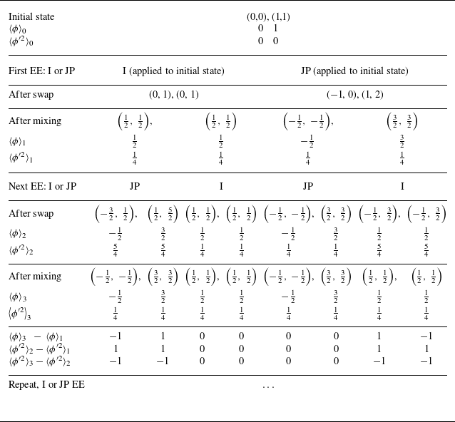
For a three-level tree, this result is obtained in Appendix D by means of exhaustive enumeration of system states and the swap-induced transitions between them.

Using the convention $\boldsymbol{\nabla }\langle \phi \rangle /(\Delta \phi _0/L_0) \equiv G=2$ in § 3.1, (3.8) and (3.9) give

(3.10) \begin{equation} \frac {D_T}{L_0^2/\tau _0} = \frac {1}{16}. \end{equation}

Importantly, (3.10) can be obtained without invoking the flux-gradient relationship. Level-0 swaps induce a random walk of fluid parcels with diffusivity $D_T=L^2/2\tau$ , where $L$ is the parcel displacement for each event and $\tau$ is the time between events. Evaluation of $L$ and $\tau$ based on the considerations that have been described recovers (3.10). Random-walk analysis is the basis of the scalar-dissipation analysis in Appendix E and is implicit in the dispersion analysis in Appendix C, which does not involve a scalar field. In Appendix B, a random-walk approach is used to analyse the HiPS molecular diffusivity. These examples illustrate the breadth of applicability of the random-walk perspective relative to the flux-gradient relationship.

The random-walk perspective likewise extends to the level-dependent turbulent diffusivity of index- $i$ swaps, yielding $D_i \propto l_i^2/\tau _i$ . For the inertial range, $\tau _i \propto l_i^{2/3}$ so $D_i \propto \tau _i^2$ . Then, in the notation of § 3.2.4, ${\rm d}\langle r^2\rangle / {\rm d}t \propto D(r) \propto t^2$ , yielding the Richardson scaling. Hence, this scaling is seen to follow directly from enforcement of $\tau _i \propto l_i^{2/3}$ in HiPS. A related explanation in terms of the HiPS dispersion formalism is provided in § 3.2.4.

3.4. Production and dissipation

In homogeneous turbulence, the scalar variance $\langle \phi ^{\prime 2}\rangle$ is given by

(3.11) \begin{equation} \frac {\partial \langle \phi ^{\prime 2}\rangle }{\partial t} = -2\langle \boldsymbol{u^\prime }\phi ^\prime \rangle \boldsymbol{\cdot }\boldsymbol{\nabla }\langle \phi \rangle -2D\langle \boldsymbol{\nabla }\phi ^\prime \boldsymbol{\cdot }\boldsymbol{\nabla }\phi ^\prime \rangle = \mathcal{P} - \langle \chi \rangle . \end{equation}

The right-hand side of this equation gives the difference between the mean scalar-variance production

(3.12) \begin{equation} \mathcal{P}=-2\langle u^\prime \phi ^\prime \rangle \boldsymbol{\cdot }\boldsymbol{\nabla }\langle \phi \rangle \end{equation}

and the mean scalar-variance dissipation rate $\langle \chi \rangle$ (Yeung & Sreenivasan Reference Yeung and Sreenivasan2014).

HiPS does not have a continuous physical domain, so calculation of production and dissipation using the standard definitions cannot be done directly. However, mean production and dissipation can be evaluated based on their roles as a scalar-variance source and sink, respectively.

Using (3.12), the first equality in (3.8), (3.9) and $\boldsymbol{\nabla }\langle \phi \rangle =2\Delta \phi _0/L_0$ , the non-dimensional production

(3.13) \begin{equation} \frac {\mathcal{P}}{(\Delta \phi _0)^2/\tau _0} = \frac {1}{2} \end{equation}

is obtained. At steady state, production and dissipation balance, and we have

(3.14) \begin{equation} \frac {\langle \chi \rangle }{(\Delta \phi _0)^2/\tau _0} = \frac {1}{2}. \end{equation}

These values were verified in HiPS simulation as follows. Production occurs due to level-0 eddies that transport fluid across the mean scalar gradient. In each half-tree, $\mathcal{P}$ is computed as the running sum of the difference in scalar variance before and after level-0 eddy events, divided by the simulation time. The values in each half-tree are then averaged. Recall that level-0 eddy events do not change the scalar values of individual parcels. The mean dissipation is computed similarly. In each half-tree, the running sum of the difference in scalar variance before and after eddies resulting in micromixing is accumulated, and this sum is then divided by the simulation time. Finally, the average of the two half-tree results is computed.

These evaluations serve to illustrate the physical fidelity of the adopted line-of-sight representation of scalar-field evolution in the imposed-mean-gradient configuration. Equation (3.12) shows that production is fully captured by such a representation. The conservative model treatment of scalar-field evolution assures that dissipation equals production. Without multiple coordinate directions in which to dissipate scalar variance, local scalar gradients must be higher by an order-unity factor than in three-dimensional physical space. Model simplifications relative to Navier–Stokes phenomenology necessarily introduce errors of this magnitude, so this artefact does not materially degrade model performance. To some extent, the artefact is subsumed in the calibration of model parameters, as in § 4. Appendix D shows an exact calculation of the production and dissipation for a three-level tree, indicating how the described phenomenology is captured in a configuration of irreducible simplicity.

Analogous considerations have been discussed in the context of the linear eddy modelling framework (Kerstein Reference Kerstein1991b ). That approach simulates scalar-field evolution on a 1-D domain that likewise represents a line of sight aligned with the mean scalar gradient. Both the present HiPS formulation and the previous LEM formulation are precise analogues of the imposed-mean-scalar-gradient configuration as studied extensively by means of DNS (Watanabe & Gotoh Reference Watanabe and Gotoh2004; Donzis, Sreenivasan & Yeung Reference Donzis, Sreenivasan and Yeung2010; Gotoh & Watanabe Reference Gotoh and Watanabe2012; Yeung & Sreenivasan Reference Yeung and Sreenivasan2014; Shete et al. Reference Shete, Boucher, Riley and de Bruyn Kops2022), theoretical analysis (Lundgren Reference Lundgren1981; Chertkov, Falkovich & Kolokolov Reference Chertkov, Falkovich and Kolokolov1998) and modeling, notably in the latter regard using the Eddy-Damped Quasi-Normal Markovian model (Briard & Gomez Reference Briard and Gomez2017) and the Lagrangian Markovianised Field Approximation (Bos Reference Bos2014).

3.5. P.d.f.s of scalar-variance dissipation rate

Unlike the evaluation of $\mathcal{P}$ and $\langle \chi \rangle$ , evaluation of the p.d.f. of $\chi$ is not uniquely prescribed on a first-principles basis. We present two approaches for its computation. The first approach makes use of the standard definition of $\chi$ given in (3.11). The gradient $\boldsymbol{\nabla }\phi ^\prime$ is computed as $\Delta \phi /\min (l^*,l_s^*)$ , where $\Delta \phi$ is the difference in scalar value between two neighbouring parcel pairs. The diffusivity $D$ is not considered directly, rather, $\chi$ is scaled so that $\langle \chi \rangle =\int \hat \chi P(\hat \chi ) \, {\rm d}\hat \chi$ , where $\langle \chi \rangle$ is evaluated as described previously.

The second approach computes $\chi$ using the following scaling: $\chi =2D\boldsymbol{\nabla }\phi ^\prime \boldsymbol{\cdot }\boldsymbol{\nabla }\phi ^\prime \sim (\Delta \phi )^2/\tau$ . Here, $\tau$ is a time scale between the micromixing events. In HiPS, we take $\tau$ to be the time since the last change of the parcel state due to micromixing events and denote this as $\tau _{tlc}$ . The $\Delta \phi$ is computed as $\tilde {\phi }-\hat {\phi }$ , where $\tilde {\phi }$ and $\hat {\phi }$ are the scalar value of a given single parcel before and after an eddy event, respectively. Then, $P(\chi )$ is constructed and we apply the same $\chi$ scaling as used in the first approach. It is found that these two approaches give nearly the same results.

Here, we present the dissipation p.d.f. using the second approach to compute $\chi$ and examine the impact of $\textit{Re}$ and $Sc$ variations. P.d.f.s of $\log _{10}(\chi )$ are shown in figure 6. Table 1 gives corresponding simulation parameters.

Figure 6(a) shows results for five $Sc$ ranging from $0.0248$ to 256 at constant $\textit{Re}$ , corresponding to a tree with $i^*=6$ and $N^*=9$ . The dissipation p.d.f.s nominally collapse for $Sc\geqslant 1$ except in the low $\chi$ tail. For these cases at constant $\textit{Re}$ , the scalar time scale $\tau _s^*$ is constant. Figure 6(b) shows results for the same $Sc$ values, but at constant Sherwood number, $Sh$ , given by

(3.15) \begin{equation} Sh = \frac {D_T}{D} = \frac {(2-A^2)Sc \textit{Re}}{8A^4}, \end{equation}

where (3.10), (B2), $\textit{Re}=A^{-\frac {4}{3}i^*}$ and $i^* = N^*-3$ are used, and use of (B2) restricts (3.15) to integer $i_s^*$ . Note that $Sh\propto Pe\equiv Sc \textit{Re}$ in HiPS. The Sherwood number is the mass-transfer analogue of the Nusselt number $Nu$ and is preferred when considering multiple scalars with unequal diffusivities. For constant $Sh$ , figure 6(b) shows collapse of the dissipation p.d.f.s for $Sc\leqslant 1$ . For $Sc\leqslant 1$ , $i_s^*$ , and hence $\tau _s^*$ and $l_s^*$ , are constant.

Table 1.

Simulation parameters corresponding to figure 6.

Figure 6.

P.d.f.s of $\log _{10}(\chi )$ for varying $Sc$ for (a) constant $\textit{Re}$ and (b) constant $Sh$ . Symbols are used for clarity to indicate p.d.f.s that collapse. For each plot, a lognormal distribution is shown with parameters corresponding to $Sc=1$ .

Analysis and modelling suggest lognormality of the dissipation rates of kinetic energy (Kolmogorov Reference Kolmogorov1962; Obukhov Reference Obukhov1962) as well as various scalar properties including the scalar variance (Gurvich & Yaglom Reference Gurvich and Yaglom1967). The latter reference introduces a simple model of scalar dissipation involving a geometric hierarchy of levels, but no representation of $Sc$ effects. It is concluded that the breadth of the p.d.f. should increase as the number of levels increases.

Such a trend is indicated in figure 6 in terms of deviation from the lognormal shape rather than lognormality per se. In both plots, the extreme rightmost tails of the p.d.f.s broaden with increasing $i_s^*$ , yet with faster than lognormal falloff in all instances.

For $Sc=1$ , similar p.d.f. shapes, including broader-than-lognormal low- $\chi$ tails, were reported by Kerstein (Reference Kerstein1991b ) based on LEM simulations and by Su & Clemens (Reference Su and Clemens2003) based on measurements in planar jets. Juxtaposed with this is the DNS result (Shete et al. Reference Shete, Boucher, Riley and de Bruyn Kops2022) shown in figure 7(a). Consistent with the HiPS set-up, the DNS case is homogeneous turbulence with a mean scalar gradient from Shete et al. (Reference Shete, Boucher, Riley and de Bruyn Kops2022). The DNS has a Taylor Reynolds number of $\textit{Re}_\lambda =633$ .

Figure 7.

(a) Dissipation p.d.f.s for $Sc=1$ and $\textit{Re}_\lambda = 559$ (HiPS); $\textit{Re}_\lambda = 633$ (DNS of Shete et al. (Reference Shete, Boucher, Riley and de Bruyn Kops2022)). (b) P.d.f.s of scalar dissipation for $\textit{Re}=256$ and Sc = 1, Sc = 256 plotted on coordinates for comparison to Chertkov et al. (Reference Chertkov, Falkovich and Kolokolov1998) for the scaling of the high $\chi$ tail. The Sc = 1 curves are shifted by 2.5 vertical-axis units for clarity.

Here, $\textit{Re}_\lambda$ for HiPS is evaluated using an analysis from Gotoh & Watanabe (Reference Gotoh and Watanabe2012). They develop a statistical theory for the scalar flux and show that $Nu \approx C_q Sc \textit{Re}_\lambda ^2$ , where the Kolmogorov constant is the only empirical input needed to obtain $C_q=0.734$ . This expression is used in HiPS, replacing $Nu$ with $Sh$ . Using (3.15) gives

(3.16) \begin{equation} \textit{Re} = \frac {8A^4}{2-A^2}C_q \textit{Re}_\lambda ^2 \approx 0.21 \textit{Re}_\lambda ^2, \end{equation}

where the final result is for $A=0.5$ . This equation completes the specification of the relationships between the parameters of the HiPS and corresponding DNS cases.

A caveat regarding (3.16) is that the accuracy of the theoretical result for $Nu$ is not firmly established. It is used as an interim procedure for relating $\textit{Re}$ to $\textit{Re}_{\lambda }$ . The $Sh$ values for DNS cases are generally not reported, but they are readily extractable from outputs, so the best future procedure is to use HiPS $Sh$ values equal to the DNS values.

Therefore, figure 7(a) shows the dissipation p.d.f. for HiPS at $\textit{Re}_\lambda =559$ for a tree with $N^*=15$ levels, along with the DNS p.d.f. and a lognormal distribution for reference. The DNS p.d.f. follows the lognormal distribution closely, except at high dissipation. The HiPS p.d.f. falls off more gradually at low dissipation and more rapidly at high dissipation. Notwithstanding this quantitative discrepancy, the HiPS high-dissipation tail exhibits a phenomenologically significant functional form, as discussed in § 3.6.

Figure 6 is plotted in non-normalised coordinates to reflect the $\textit{Re}$ and $Sc$ dependencies on low moments (mean and variance) of the p.d.f.s. DNS studies generally show only normalised p.d.f. with no separate reporting of the low moments. The novel capability of HiPS to predict these quantities motivates an ongoing effort to acquire the relevant data for comparison purposes, results of which will be reported elsewhere.

3.6. High-dissipation phenomenology

Holzer & Siggia (Reference Holzer and Siggia1994) studied passive scalar mixing in two dimensions and found good agreement with experimental data in more complex configurations. They show that a stretched-exponential function fits the dissipation p.d.f. in the large-dissipation tail. Chertkov et al. (Reference Chertkov, Falkovich and Kolokolov1998) analysed high- $Sc$ scalar advection using the Kraichnan (Reference Kraichnan1974) model. They derived an expression for $P(\chi )$ , which can be represented as $\log (P(\chi )\chi ^{1/2})\propto \chi ^{1/3}$ . For $\chi \gg \langle \chi \rangle$ , the p.d.f. is given by a stretched exponential, with $\log P(\chi )\propto \chi ^{1/3}$ .

Figure 7(b) shows $\log _{10}(P(\chi )\chi ^{1/2})$ and $\log _{10}(P(\chi ))$ versus $\chi ^{1/3}$ for HiPS at $\textit{Re}=256$ and $Sc=1$ , $Sc=256$ . Note that the $Sc=1$ curves have been vertically shifted for clarity. Linear fits through the 12 largest $\chi$ values are shown, corresponding to Chertkov’s model in the coordinates plotted. It is seen that for both Schmidt numbers, the HiPS data reproduces the predicted $1/3$ exponent. Moreover, the fit is better when the subdominant $\chi ^{1/2}$ factor is included, indicating the possibility that the model captures this dependence.

The $1/3$ exponent for $Sc = 1$ is unexplained beyond speculative proposals although it has prior empirical support (Chertkov et al. Reference Chertkov, Falkovich and Kolokolov1998). It is additionally supported by recent DNS results (Dotson, Yeung & Sreenivasan, unpublished).

Insofar as the Chertkov et al. (Reference Chertkov, Falkovich and Kolokolov1998) analysis is applicable at least at high $Sc$ , it embodies the distant interactions between Kolmogorov eddies and much smaller scalar structures in the viscous-advective regime. As explained in § 1, the HiPS representation of this regime likewise embodies that phenomenology, perhaps hinting at common features of the analysis and the model whose elucidation could clarify the significance of the $1/3$ exponent. Apart from the specific exponent value, the broader question of the phenomenological origin of the stretched-exponent tail of the HiPS p.d.f. is addressed in Appendix E.

3.7. Scalar spectra

Scalar transport in turbulent flow is commonly represented and analysed using the scalar variance spectrum. A detailed interpretation of the scalar variance spectrum in the context of HiPS was provided by Kerstein (Reference Kerstein2013), but no computations were performed. Here, we provide a summary description and computations of the scalar spectrum for various Schmidt numbers.

In HiPS, the scalar variance spectra are inferred from the differences of scalar variances at adjacent levels of the tree. As noted by Kerstein (Reference Kerstein2013), the quantity $\int _\kappa ^\infty E(\kappa ^\prime )\,{\rm d}\kappa ^\prime$ ‘scales as the variance of scalar fluctuations associated with wavenumbers exceeding $\kappa$ ’, so to evaluate the integral and ultimately $E(\kappa )$ , the wavenumber-restricted variance is first evaluated. The tree structure of HiPS has discrete, geometrically decreasing length scales with increasing tree level. We can think of each level $i$ of the tree as having a corresponding wavenumber $\kappa _i$ with $l_i = 2\pi /\kappa _i$ . A discrete scalar spectrum is then given by

(3.17) \begin{equation} E(\kappa _i) = \frac {\text{var}_{i}\phi - \text{var}_{i+1}\phi }{\kappa _{i+1}-\kappa _i}. \end{equation}

As $A$ approaches unity, this converges to the familiar continuum relationship between the scalar spectrum and the variance of the filtered scalar field, assuming spectrally sharp filtering.

Scalar spectra are obtained for three mixing regimes: inertial-advective, inertial-diffusive and viscous-advective. Figure 8 shows scalar spectra from HiPS simulations over a range of Schmidt numbers.

The inertial-advective regime is characterised by turbulent scalar transport with negligible diffusive effects and spectral transfer from large to small scales is governed by the scalar-variance dissipation rate $\chi$ , which is independent of the length scale. The increasing advective rate with decreasing length results in quasi-stationary behaviour that responds quickly to scalar variance transferred from larger scales. In this regime, time scales are related to length scales as $\tau \sim l^{2/3}$ and the kinetic-energy spectrum exhibits $\kappa ^{-5/3}$ scaling. In HiPS, this time scale–length scale relationship is imposed, but as Kerstein (Reference Kerstein2013) notes ‘scalar cascading in HiPS is an outcome rather than a prescribed behaviour, so the nature of that cascading in HiPS must be ascertained’. It is seen that HiPS does in fact exhibit the –5/3 wavenumber power-law of the scalar spectrum. While HiPS does not prescribe the cascading behaviour, its formulation is consistent with it, as HiPS subsumes the key phenomenology that governs it. This is evident as HiPS eddies result in local scale reduction, the eddy rate increases with decreasing level length giving quasi-stationary behaviour, and the HiPS eddies are non-dissipative at all scales greater than $l^*$ .

Figure 8.

Scalar variance spectra for (a) $Sc\geqslant 1$ and (b) $Sc\leqslant 1$ .

Figure 8(a) shows simulations for scalars with $Sc\geqslant 1$ . Six $Sc$ values are included. These have $Sc$ = 1, 4, 16, 64, 256, 1024, corresponding to integer values of $\Delta i = i_s^*-i^*$ from 0 to 5, see (2.19). The simulation has a total of 12 levels and $i^*=4$ . This accommodates both a significant wavenumber range of the inertial-advective regime and extension to smaller scales ( $i \gt i^*$ ) for $Sc \gt 1$ . The simulations were run for $t=1000\tau _0$ , and flow states spaced by time intervals $\tau _0$ were processed beginning with $50\tau _0$ .

All spectra show a clear transition between the inertial-advective regime and the viscous-advective regime, and they all obey the $-5/3$ scaling at low wavenumbers. In the viscous-advective regime $i\gt i^*$ , the spectra show the expected $\kappa ^{-1}$ scaling. This is most obvious for the scalars with the highest $Sc$ .

In the simple micromixing model used in this study, immediately after a swap occurs at level $i_s^*$ , all parcels in the left subtree of the node at the given eddy level are mixed to their mean value in that subtree; all parcels in the right subtree are similarly mixed. This results in no scalar variance among parcels at levels greater than $i_s^*$ , so the scalar variance spectrum is effectively chopped at length scales below $l^*$ , corresponding to levels $i \gt i_s^*$ . As formulated, this eliminates the need to implement any eddy events at levels $i \gt i_s^*$ because they would have no effect.

This, however, provides an inadequate representation of the inertial-diffusive scaling range, for which Batchelor (Reference Batchelor1959) predicted a $-17/3$ spectral scaling. This scaling was demonstrated by Chasnov & Rogallo (Reference Chasnov and Rogallo1988) and Chasnov (Reference Chasnov1991) using simulations of scalar transport in a frozen, Gaussian, isotropic velocity field, and in LES of decaying and forced turbulence. More recently, DNS by Yeung & Sreenivasan (Reference Yeung and Sreenivasan2013, Reference Yeung and Sreenivasan2014) found the $-17/3$ spectral scaling in forced homogeneous isotropic turbulence with an imposed mean scalar gradient.

Accordingly, the $Sc \lt 1$ eddy event, which performs the described mixing if the event level is $i_s^*$ , is modified to approximate the theoretical spectral scaling in lieu of the sharp cutoff at level $i_s^*$ . Instead of assuredly mixing the respective two subtrees of the level- $i_s^*$ event apex, for any eddy event at level $i\geqslant i_s^*$ , both the left and right subtrees of the event apex are individually mixed with probability $p$ based on a Bernoulli trial. This allows scalar fluctuations to persist below the Obukhov–Corrsin scale. At level $j \gt i_s^*$ , we then have an inhomogeneous scalar fraction $q^j$ where $q=1-p$ . The scalar variance then would be $q^j$ times what it would be in a $-5/3$ spectrum. Here, it is assumed that the inertial-advective cascade proceeds as usual in the successive generations of unmixed subtrees, which requires the re-introduction of eddy events at levels $j \gt i_s^*$ where such events can change the system state (versus the absence of such events for $q=0$ ). Recalling that spectral amplitude scales in proportion to the scalar variance, the -17/3 power-law spectrum scaling is obtained by imposing the requirement

(3.18) \begin{equation} \frac {E_j}{E_{i_s^*}} = \frac {\text{var}_j\phi }{\text{var}_{i_s^*}\phi }=q^j\left (\frac {\kappa _j}{\kappa _{i_s^*}}\right )^{-5/3} = \left (\frac {\kappa _j}{\kappa _{i_s^*}}\right )^{-17/3}. \end{equation}

Now, $l^*_s/l_j=2^j$ , so $\kappa _j/\kappa _{i_s^*}=2^j$ and $j=\log _2(\kappa _j/\kappa _{i_s^*})$ . Using this and solving (3.18) for $q$ gives $q=2^{5/3-17/3}=0.0625$ and $p=1-q=0.9375$ . This result is approximate because it is based on strict mean-field Kolmogorov phenomenology, omitting fluctuation effects such as backscatter (discussed with reference to the viscous-advective regime) that are inherent to HiPS.

Therefore, figure 8(b) shows simulation results for $Sc\lt 1$ in the inertial-diffusive regime. Each case again includes 12 tree levels and was run for the same time with the same number of flow states processed as the cases shown in figure 8(a). That figure had $i^*=4$ for $Sc=1$ , with higher levels accommodating larger $Sc$ . For $Sc\lt 1$ in figure 8(b), $i^*=9$ for $Sc=1$ (with levels starting at 0), and $Sc=$ 1, 0.397, 0.157, 0.0625, 0.0248 and 0.098 (rounded), corresponding to $\Delta i=i_s^*-i^*$ from 0 to -5, respectively. The slopes in the inertial-diffusive regime are slightly steeper than –17/3, but they can be brought into agreement with this exponent by using a slightly lower value of $p$ (around 0.9).

Here, $p\lt 1$ allows gradual imposition of homogeneity to compete with swap-induced introduction of inhomogeneity such that the balance can be tuned to reproduce –17/3 scaling. This compensates for the underlying instantaneous nature of state changes in the model, a model artefact that introduces a splitting error. LEM is subject to a comparable artefact, producing an exponent error that has been explained quantitatively (Kerstein Reference Kerstein1991b ), but the LEM formulation does not accommodate a convenient correction.

The scalar spectra discussed here and plotted in figure 8 are discrete. As an alternative formulation, we can evaluate continuous spectra in the inertial-advective regime, which is convenient for analysis. This is done using a power-law with an exponent of $-5/3$ , consistent with the presented spectra. The power-law amplitude is set so that the integral of the continuous spectra, extending to level 1 corresponding to $L_I$ , recovers the total variance. Using such continuous spectra, we denote the compensated spectrum $E\kappa ^{5/3}$ as $E_{\kappa 53}$ ; its non-dimensional value is

(3.19) \begin{equation} \frac {E_{\kappa 53}}{\Delta \phi _0^2/L_0^{2/3}} = 4.3. \end{equation}

This is based on a simulation with $N_t=12$ levels and $Sc=1$ , but applies generally given the collapse of the scalar spectra in the inertial-advective range, evident in figure 8.